Estimation of geoacoustic parameters and source range using airgun sounds in the East Siberian Sea, Arctic Ocean

Dispersion is a representative property of low-frequency sound propagation over long distances in shallow-water waveguides, making dispersion curves valuable for geoacoustic inversion. This study focuses on estimating the geoacoustic parameters using the dispersion curves extracted from airgun sounds received in the East Siberian Sea. The seismic survey was conducted in September 2019 by the icebreaking research vessel R/V Araon, operated by the Korea Polar Research Institute. A single hydrophone was moored at the East Siberian Shelf, characterized by nearly range-independent shallow water (<70 m) with a hard bottom. In the spectrogram of the received sounds, the dispersion curves of the first two modes were clearly observed. Utilizing a combination of warping transform and wavelet synchrosqueezing transform these two modes were separated. Then, the geoacoustic parameters, such as sound speed and density in the sediment layer, were estimated by comparing the two modal curves extracted at a source-receiver distance of approximately 18.6 km with the predictions obtained by the KRAKEN normal-mode propagation model. Subsequently, the distances between the airgun and the receiver system in the 18.6 to 121.5 km range were estimated through the comparison between the measured modal curves and the model replicas predicted using the estimated geoacoustic parameters.

1 Introduction

The East Siberian Sea remains one of the least studied areas in the Arctic Ocean due to its harsh climate characterized by heavy sea ice conditions. The topography of the East Siberian Shelf, located between the Chukchi Sea and the Laptev Sea, consists of a flat and shallow hard-bottom region that gradually slopes from southwest to northeast (Jakobsson et al., 2020). Approximately 70% of the waters have a water depth shallower than 50 m, with an average water depth of ~58 m (Outridge et al., 2008). Previous studies reported that the East Siberian Shelf is primarily composed of cemented subsea permafrost, which refers to a permanently frozen sedimentary layer (Brown et al., 1997; Romanovskii, 2004). This permafrost is overlaid by a relatively soft surficial layer consisting of a mixture of silt, sand, and stones (O’Regan et al., 2017; Jin, 2020; Han et al., 2023). As global warming accelerates in the Arctic region, significant environmental changes are occurring in the Arctic Ocean, leading to drastic changes in the underwater acoustic environment (Frisk, 2012; Mahanty et al., 2020; Duarte et al., 2021).

As part of research on these changes in the ocean environment, we have recently published two papers that present the outcomes of our studies on the underwater acoustical environment in the East Siberian Sea. In the first paper, Han et al. (2021) conducted measurements of long-term acoustic ambient noise in the East Siberian continental margin for a year, spanning from August 2017 to August 2018. Our analysis revealed that the spectrum level varied with seasons, exhibiting a strong negative correlation with changes in the sea ice concentration covering the sea surface. This pattern is likely attributed to increased ambient noise level due to exposure to underwater noise sources such as wind and rainfall as the sea ice on the sea surface melts in the summer. In addition, the utilization of airgun in seismic surveys in regions where sea ice has melted also contributed to the increase of ambient noise level. For example, during the one-year measurement period, the lowest sea ice concentration was in September, and underwater ambient noise during this period was approximately 16 dB higher than the annual average.

Underwater noise measurements were conducted again in the same region as the first measurement for about a year from August 2019 (Han et al., 2023). Additionally, from September 2 to 10, the R/V Araon, operated by the Korea Polar Research Institute (KOPRI), conducted a seismic airgun survey for underwater geological exploration. During this period, the airgun sounds at different source-receiver distances were unintentionally received by the receiver system. The received levels as a function of distance were compared with model predictions obtained from a broadband application of the range-dependent acoustic model (RAM) (Collins, 1993) based on the parabolic equation (PE). A two-layer geoacoustic bottom model, which was constructed based on core samples and sub-bottom profile survey data, was used as model input. The uppermost layer of the two-layer model was set to be mud composed of soft unconsolidated sediment less than 4 m thick with a sediment sound speed range of 1,424−1,471 m/s, sediment density range of 1.39−1.53 g/cm³, and sediment attenuation coefficient range of 0.0793−0.1532 dB/λ, which are estimated using the geoacoustic relationships with mean grain size (Ainslie, 2010). The lower layer was set to the diamicton, of which the sound speed, density, and attenuation coefficient ranges were assumed to be 1,588−1,928 m/s, 1.82−2.55 g/cm³, and 1.1006−0.9076 dB/λ, respectively. However, there was a significant difference between the measurements and the predictions, which became the motivation of this study. In this paper, the geoacoustic parameters of the site are estimated by comparing modal dispersion curves derived from the acoustic model predictions and the measurements.

In shallow water environments, long-range acoustic propagation is greatly influenced by geoacoustic parameters such as sound speed and density of the seafloor. Low-frequency sounds propagating over several kilometers in the ocean waveguides are dispersive in the time-frequency domain, which can be explained with normal mode theory as the sum of several modal components (Frisk, 1994; Jensen, 2011; Duncan et al., 2013; Keen et al., 2018). For this reason, the modal dispersion curves to be observed at the time-frequency domain of the received signal reflects the acoustic properties of the ocean waveguide, including the geoacoustic parameters, and therefore, it can be used to estimate the geoacoustic properties of the seafloor. In order to use the dispersion curves for geoacoustic parameter inversion, it is necessary to extract the dispersion curves for each mode from the spectrogram of the received signal, and then compare them with the simulated replicas obtained by the normal-mode-based propagation model. Recently, since warping transform was proposed as a good tool used for extracting the dispersion curves in the spectrogram (Bonnel et al., 2020), it has been applied to geoacoustic inversion studies in shallow water using various low-frequency broadband sound sources such as airgun, gunshot, light bulb, and whale call (Bonnel et al., 2013; Warner et al., 2015; Duan et al., 2016; Warner et al., 2016; Thode et al., 2017; Liu et al., 2020).

In this paper, we present the results of estimating geoacoustic parameters of the seafloor in the East Siberian Shelf. The modal dispersion curves of the first two modes were clearly observed in the spectrogram of the airgun sounds received at distances of several tens of km, and they were extracted using the warping transform combined with the wavelet synchrosqueezing transform. The genetic algorithm (Goldberg, 1989; Conn et al., 1997) was then applied to find the best-fit geoacoustic parameters by matching the extracted dispersion curves with the replicas predicted by the KRAKEN normal-mode program (Porter, 1992) within the search spaces of the geoacoustic parameters. Additionally, our geoacoustic inversion results were used to estimate the distance of sound source for distances from 18.6 km to 121.5 km.

2 Materials and methods

2.1 Acoustic measurements

Long-term underwater noise measurements were conducted in the East Siberian Shelf over the course of approximately one year, spanning from August 22, 2019 to August 13, 2020. An autonomous passive acoustic recorder (AURAL-M2, Multi-Electronique Inc.) was moored 13 m above the seafloor at location 74° 37.327’N, 174° 56.397’E in waters with a depth of approximately 70 m (Figure 1A). Acoustic data were recorded for 10 minutes every hour at a sampling rate of 32,768 Hz. From September 2 to 10, 2019, the R/V Araon operated the airgun (GI-SOURCE 355, Sercel) for underwater geological survey in the Chukchi-East Siberian Continental Margin (Jin, 2020). Low-frequency impulsive airgun sounds were emitted by the airgun shots at approximately 11-s intervals while maintaining a constant firing depth of ~6 m. The waveform of the airgun shot, measured from a near-field hydrophone (AGH-7100-C, Geophysical Products Inc.) positioned approximately 1 m above the airgun, exhibited a spike-shaped pattern with a peak frequency of ~27 Hz and dominant energy concentrated below 300 Hz (Han et al., 2023).

Figure 1

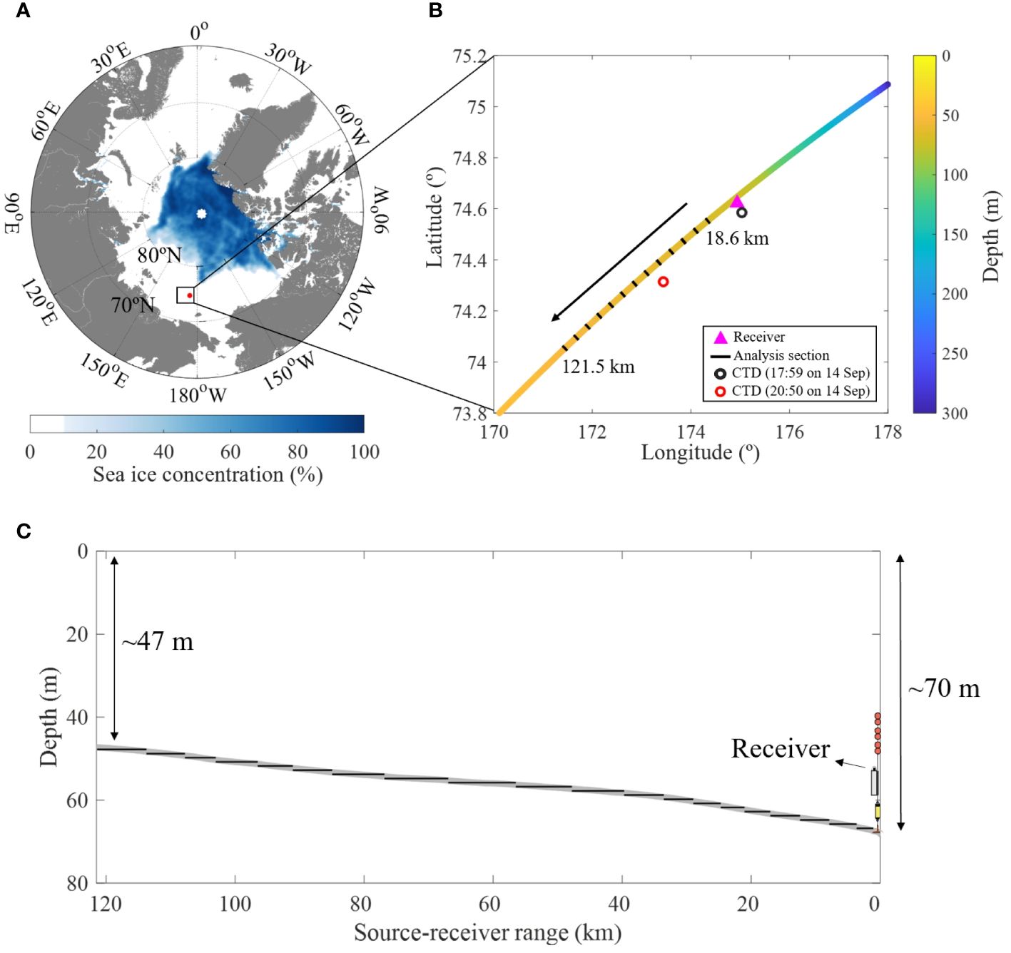
Figure 1 (A) Distribution map of sea ice concentration in the Arctic on September 9, 2019. Black box denotes the location of the measurement site. (B) The R/V Araon ship track. The colors on the ship track indicate bathymetry. The magenta triangle denotes the hydrophone mooring location, and the black and red open circles show the CTD cast locations. Acoustic data received at 18.6 km was applied to geoacoustic inversion, and the 13 sections (approximately 50 signals per section), represented by black bars on the ship tracks, were used to estimate the distance from the receiver system to sound source. (C) Range-dependent bathymetry along the source-receiver track. Black solid lines represent the range-independent segments, each based on a 1-m change in water depth.

During the seismic survey, the R/V Araon approached the receiver system from the northeast direction, coming closest at 15:47 on September 9, after which the vessel moved away in the southwest direction (Figure 1B). Notably, bathymetry in the northeast direction from the receiver exhibited range-dependent variations, while bathymetry in the southwest direction displayed minimal changes in water depth. Our current analysis focused on cases where the source moved away from the receiver in the southwest direction within a range-independent environment. It is important to note that when the source-receiver distance was less than 18.6 km, the energy of received signal exceeded the upper dynamic limit of the hydrophone, leading to signal truncation. Moreover, airgun data received at distances exceeding 121.5 km exhibited poor signal-to-noise ratio (SNR). Therefore, our analysis was confined to the range encompassed between these two distances.

2.2 Extraction of dispersion curves

Acoustic waves propagating in a waveguide exhibit dispersion as normal modes at different frequency propagate at different group velocities. Therefore, several dispersive modes with different frequency-dependent group velocities can be observed in the spectrogram of the received signal after propagating at least several kilometers in shallow water, and the group velocity $v_m(f)$ is calculated by Equation 1 (Frisk, 1994; Jensen, 2011; Bonnel et al., 2020):

$\begin{array}{ll}{v}_m(f)=2\pi \frac{\partial f}{\partial k_m(f)}& (1)\end{array}$

where, $k_m(f)$ is the horizontal wavenumber of mode m at frequency f. Therefore, the modal travel time t_m as a function of frequency over propagation range r is given by

$\begin{array}{ll}{t}_m(f)=\frac{r}{v_m(f)}& (2)\end{array}$

Figure 2A shows the time series of the airgun sound received at a source-receiver distance of 18.6 km. Interestingly, arrivals that appear to be precursor arrivals were received before the water-borne arrivals. The precursor arrival is a signal that propagates primarily through the sediment layer and arrives prior to any water-borne arrival (Dahl and Choi, 2006; Choi and Dahl, 2007), and the observation of precursor arrivals in our measurements means that the sound speed in lower sediment layer might be faster than that in the water column. Figure 2B shows the spectrogram for water-borne arrivals corresponding to the red box in Figure 2A. The first two modes were clearly observable in the spectrogram. However, higher modes were not clearly visible.

Figure 2

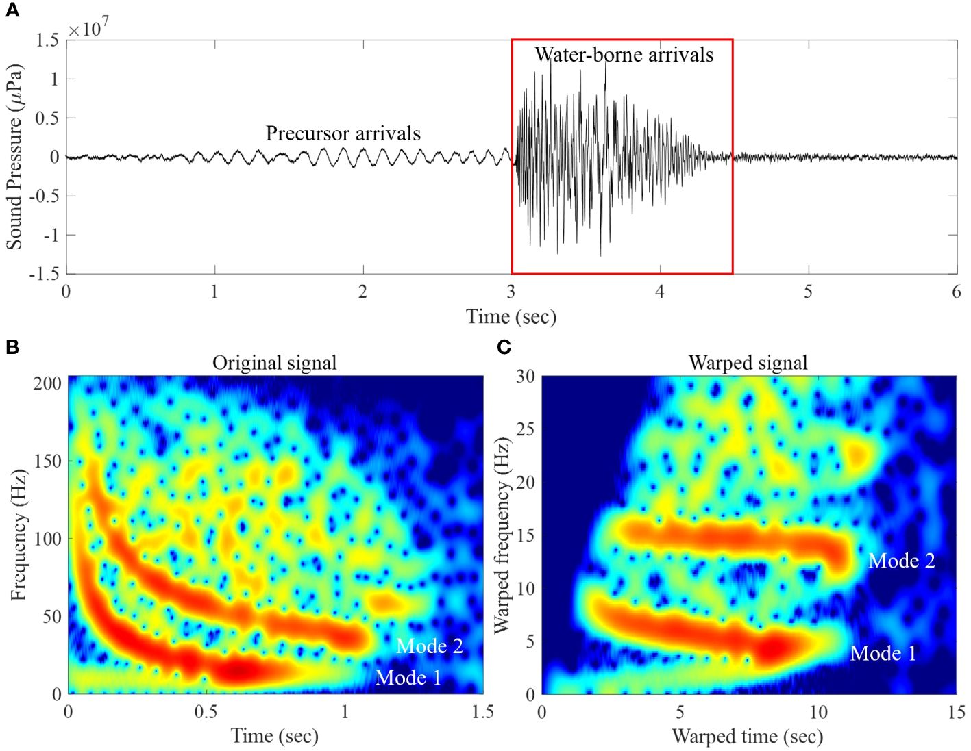
Figure 2 (A) Time series of the airgun sound received at the source-receiver distance of 18.6 km. (B) The spectrogram of the water-borne waveforms corresponding to the red box in (A), which was obtained by the short-time Fourier transform using 512 fast Fourier transform points and 51-point Hamming window after decimation by a factor of 80. (C) Spectrogram of the warped signal.

In this study, the warping method was applied to extract each dispersion curve from the spectrogram. In normal mode theory, for an impulsive source signal propagating in a Pekris waveguide with a rigid bottom, the received signal as a function of time t can be expressed as (Jensen, 2011; Bonnel et al., 2020)

$\begin{array}{ll}\text{y}(t)={\displaystyle \sum _{m=1}^M}{a}_m(t)e^{j2\pi f_{cm}\sqrt{t^2-{(\frac{r}{c_w})}^2}}& (3)\end{array}$

where M is the mode number of propagating modes, a_m is the amplitude of mode m, c_w is the water sound speed, and f_cm represents the cutoff frequency of the m-th mode which can be calculated by $\frac{(2m-1)c}{4D}$, where D is the water depth. Note that the phase term of (Equation 3) is a non-linear function for time t. To linearize the non-linearity, we used $\sqrt{t^2+{(\frac{r}{c_w})}^2}$ as the warping function h(t) under the assumption that the impulsive source signal propagates in an isovelocity waveguide. The warped signal y_w(t) is calculated by

$\begin{array}{ll}{y}_w(t)=\sqrt{\left|h^{\prime }(t)\right|}y[h(t)]& (4)\end{array}$

where h(t) is the warping function, $h^{\prime }(t)$ is the time derivative of h(t) (Bonnel and Chapman, 2011; Bonnel et al., 2020; Liu et al., 2020). Figure 2C shows the result of the warping transformation, in which the first two modes are well separated in the warped frequency.

Now that the two modes have distinct warped frequency bands, we extracted the first and second modes using a bandpass filter, as shown in Figures 3A, B, respectively. Each warped modes were then inversely warped by replacing h(t) with $h{(t)}^{-1}$= $\sqrt{t^2-{(\frac{r}{c_w})}^2}$ in (Equation 4). As a next step, wavelet synchrosqueezing transform was applied to sharpen the time-frequency resolution of the dispersion curves of each mode (Daubechies et al., 2011; Thakur et al., 2013), and then time-frequency ridge tracking algorithm (Meignen et al., 2015; Iatsenko et al., 2016) was used to extract the maximum-energy ridges from wavelet synchrosqueezing transform results, and the results are shown in Figures 3C, D. Finally, the extracted dispersion curves were smoothed out using a 5-point moving average filter, with the results shown as red dashed lines in Figures 3C, D.

Figure 3

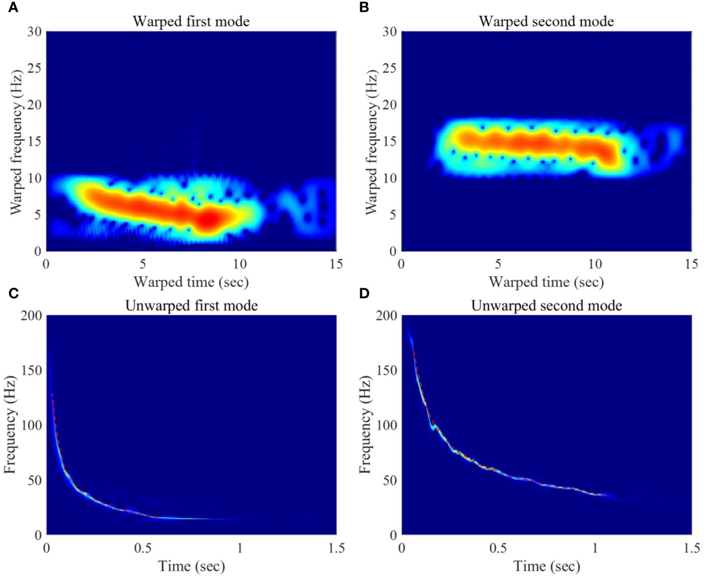
Figure 3 (A) Spectrograms of the warped first and (B) second modes extracted through bandpass filtering. (C) Dispersion curves obtained by the wavelet synchrosqueezing transform of the inverse-warped first and (D) second modes. Red dashed lines are the 5-point moving averaged output of the dispersion curves.

2.3 Geoacoustic inversion

The seafloor of the experimental site was flat with a water depth difference of only ~5 m from the receiver position to a point 18.6 km southwest. The sediment structure was reported to be composed of a thin layer of unconsolidated mud overlying the high-density sediment created by the grounding events of ice masses through the repeated advance and retreat of glaciers (Niessen et al., 2013; Dove et al., 2014; Han et al., 2023). The sound speed profile in the water column was measured using a conductivity-temperature-depth (CTD) cast on 14 September at points ~5 and ~56 km from the receiver (see the black and red open circles in Figure 1B), and the measurements showed that the sound speed profiles at two points were similar and distributed within the range of 1,438 and 1,448 m/s (Figure 4A).

Figure 4

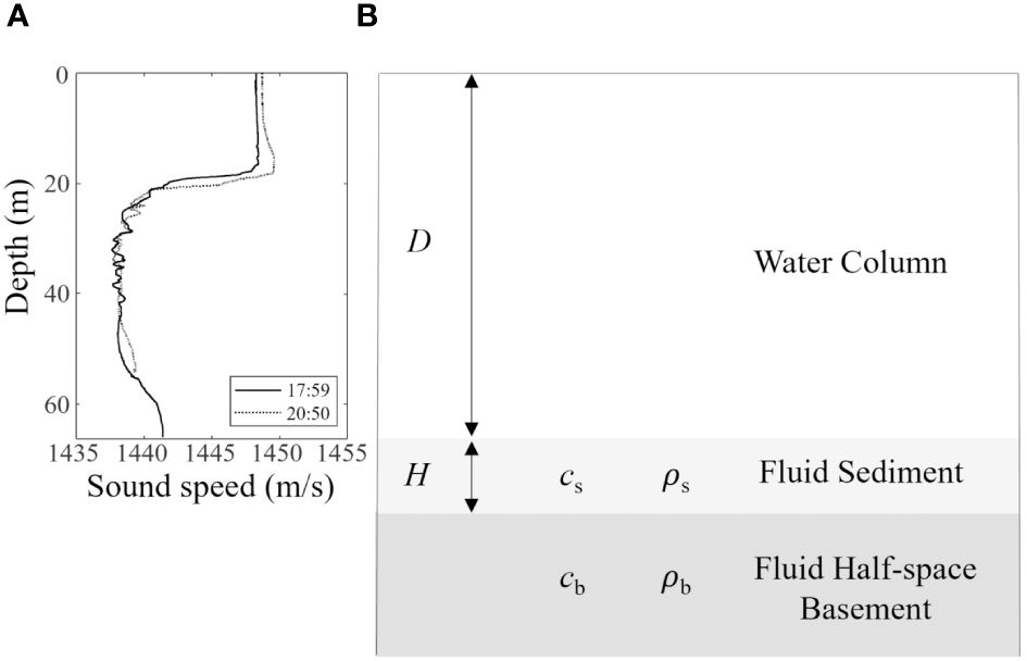
Figure 4 (A) Sound speed profiles at points ~5 (solid line) and ~56 km (dashed line) southwest of the receiver, which were measured at 17:59 and 20:50 on 14 September, respectively. (B) Two-layer geoacoustic bottom model constructed for the geoacoustic inversion process.

In this study, a two-layer bottom model for geoacoustic parameter inversion was constructed based on the previous survey results (Han et al., 2023), as shown in Figure 4B. It was assumed that the ocean environment is range-independent, and the bottom consists of a homogeneous fluid sediment layer overlying a homogeneous fluid half-space. The genetic algorithm was used to estimate geoacoustic parameters by matching the extracted dispersion curves from the acoustic data with the replicas predicted by the KRAKEN acoustic propagation model. As mentioned in Section 2.1, the shortest range from the receiver position where the received signals were not truncated was 18.6 km, and at which point the water depth difference between the receiver and airgun positions was only ~ 5 m. Therefore, we used the data received at this point for geoacoustic parameter inversion.

Based on the two-layer bottom model, we estimated six unknown parameters including the layer thickness H, sound speed c_s and density ${\rho }_s$ in the surficial sediment layer and sound speed c_b and density ${\rho }_b$ of the basement, and the water depth D. The sound speed profile measured at the point ~5 km from the receiver position was used as model input to run the KRAKEN acoustic propagation model. The search spaces for each parameter are shown in Table 1, which were set to sufficiently wide ranges based on previous survey results (Han et al., 2023). To create model replicas, the KRAKEN model was run in the frequency range between 16 and 130 Hz for mode 1 and 36 and 170 Hz for mode 2 at a 1-Hz interval. Then, the group velocity predictions as a function of frequency were converted to modal travel time for the source-receiver distance of 18.6 km by (Equation 2). To compare the modal travel times between the model replicas and those extracted dispersion curves from the acoustic data, each result was time-aligned by adjusting the arrival time for 130 Hz of the first mode to 0 on the time axis. Then, the least square method was used, in which the objective function to be minimized is given by

Table 1

Table 1 Search spaces and estimated optimal parameter values for environmental parameters applied in geoacoustic inversion in the range-independent environment.

$\begin{array}{ll}J(\text{X})={\sum }_{m=1}^M{\sum }_{n=1}^{N_m}{[t_m(f_n)-{\widehat{t}}_m(f_n,\text{ X})]}^2& (5)\end{array}$

where M is the total number of modes used for the geoacoustic inversion, and M was set to 2 in this study. The vector $\text{X}=\{H,c_{\text{s}},{\rho }_{\text{s}},c_{\text{b}},{\rho }_{\text{b}},D\}$. $t_m(f_n)$ and ${\widehat{t}}_m(f_n,\text{ X})$ is the measured and modeled modal travel times, respectively. N_m is the total number of frequency segments used for the mode m.

To determine the optimal values of geoacoustic parameters, a global search was conducted using a genetic algorithm over the parameter search spaces. The genetic algorithm parameters were set as follows: a population size of 64, a crossover fraction of 0.8, and a mutation probability of 0.05 to prevent local minima. The algorithm terminated either when the number of generations reached 300 or when the objective function no longer decreased within an additional 60 generations from the generation that achieved the best result.

3 Results

3.1 Inversion in range-independent environment

The best-fit values and their uncertainties for each parameter within the search space are presented in Table 1. The inversion results reveal a water depth of approximately 68.2 m, with a surficial sediment layer approximately 4.1 m in thickness overlaying a high-velocity basement. The surficial sediment exhibits an approximate sound speed of 1422.4 m/s and a density of about 1.58 g/cm³. These results suggest that the estimated geoacoustic parameters of the surficial sediment layer closely align with our previous survey results (Han et al., 2023). Additionally, the underlying basement displays a sound speed of approximately 1733.6 m/s and a density of approximately 1.84 g/cm³. Figure 5 shows the sensitivities of $J(\text{X})$ to parameter variations around the optimal values of the six environmental parameters. A sensitivity plot for each parameter is created by calculating $J(\text{X})$ within the search spaces while keeping other parameters at their optimal values. As expected, $J(\text{X})$ is most sensitive to the sound speed of the lower sediment layer and water depth D, while the other parameters are relatively less sensitive in the inversion process. In the sensitivity results for the surficial layer thickness, 0 m represents a scenario where the sediment is not structured with two sediment layers but solely with a half-space. Figure 6 compares the measured modal curves with model replicas predicted using the inversion results for the first four modes. Although the mode-3 and 4 are not clearly visible in the measured spectrogram, the predictions of mode-1 and 2 are in good agreement with the corresponding measured modal curves.

Figure 5

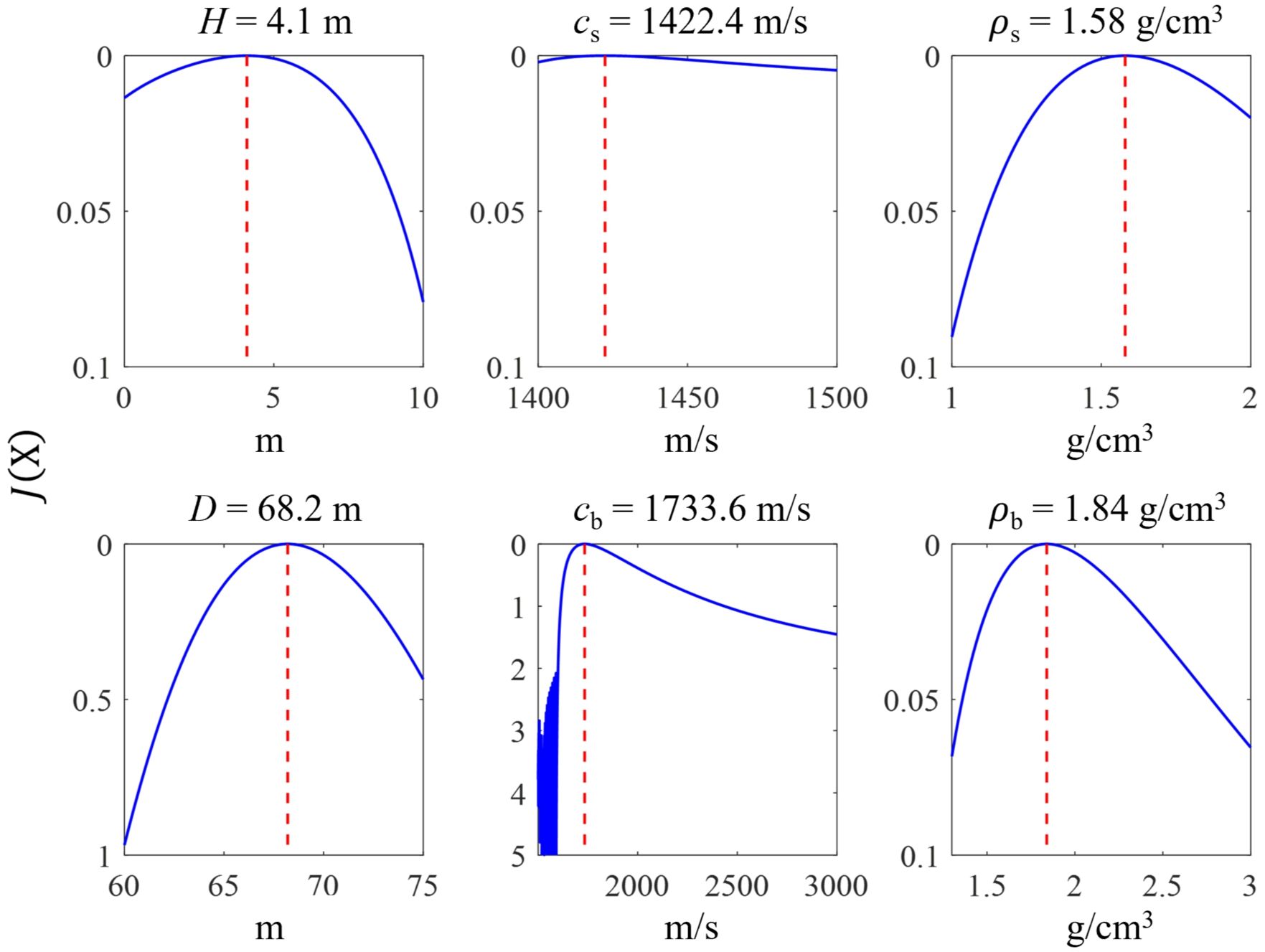
Figure 5 Sensitivity plots for each geoacoustic parameter. Red dashed lines are optimal values for each geoacoustic parameter. Note that the $J(\text{X})$ scales of the c_b and D is different from those of other parameters.

Figure 6

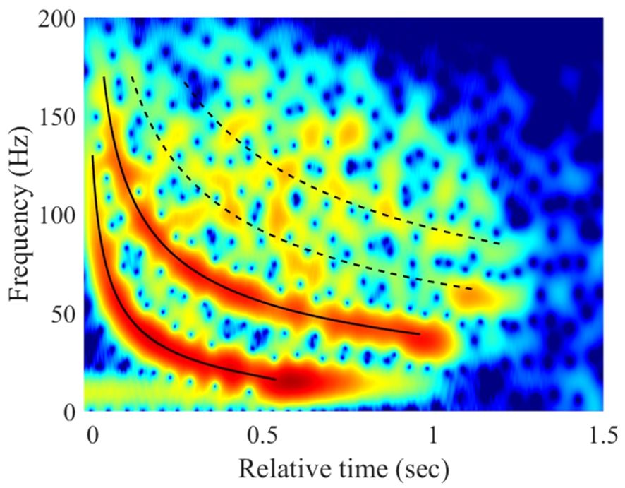
Figure 6 Comparison of dispersion curves between the modal curves in the measured spectrogram and the model replicas predicted using the estimated geoacoustic parameters. Black solid lines indicate the model replicas for the mode-1 and 2, which were used for the inversion process, and black dashed lines indicate the model replicas for mode-3 and 4.

As a subsequent step, the Bayesian approach was applied to estimate the uncertainties in geoacoustic parameter estimates derived from the inversion process. Let X and d denote the given vectors representing the six geoacoustic parameters and the measured data, respectively. Following Bayes’ rule, the posterior probability density $P(\text{X|}d)$ can be expressed as Equation 6 (Gerstoft and Mecklenbräuker, 1998; Dosso, 2002; Dosso and Dettmer, 2011)

$\begin{array}{ll}P(\text{X|}d)=\frac{P(d|\text{X})P(\text{X})}{P(d)}& (6)\end{array}$

where $P(\text{X})$ is the prior distribution, and $P(d\text{|X})$ is the conditional probability density of given vector X for the measured data d. $P(d)$ is the probability density of measured data d, acting as a normalizing factor. To calculate $P(\text{X|}d)$, the prior distribution is assumed to be uniform within the search bounds of each parameter. The conditional probability density $P(d\text{|X})$, interpreted as the likelihood function L(X), is given by Equation 7

$\begin{array}{ll}P(d\text{|X})=L(\text{X})\propto \exp [-J(\text{X})]& (7)\end{array}$

where $J(\text{X})$ represents the data misfit function (considered in section 2.3). Consequently, the posterior probability density can be written as Equation 8

$\begin{array}{ll}P(\text{X|}d)=\frac{\exp [-J(\text{X})]}{\int \exp [-J(\text{X})]\text{dX}}& (8)\end{array}$

In this study, the Markov-chain Monte Carlo method utilizing Metropolis sampling (Metropolis et al., 1953; Hastings, 1970) was employed to estimate the marginal probability densities for each parameter. The inversion results were then utilized as initial values for the estimation. The sampling process involved 10,000 iterations using a proposal distribution in the form of a normal distribution, centered on the sampled results. Considering the parameter scale, the standard deviation of the proposal distribution for sound speed parameters was set to 1, while for the remaining parameters, it was set to 0.1. Subsequent to estimating the marginal probability densities for each parameter, parameter uncertainties were quantified using 95% Highest Probability Density (HPD) credible intervals (Bonnel et al., 2013; Gelman et al., 2013), as depicted in the last right column of Table 1.

Up to this point, we have derived estimates for geoacoustic parameters and water depth by comparing measured modal curves with model replicas for a source-receiver distance of 18.6 km. Conversely, if ocean environmental parameters, including geoacoustic parameters, are assumed to be known, the distance between the acoustic source and receiver can be estimated using the same method as described above. As indicated in section 2.1, reliable signals were received within the range of 18.6 and 121.5 km. Therefore, in this session, we estimate source-receiver distances for this range. Initially, assuming a range-independent environment, we executed the KRAKEN acoustic propagation model with input parameters comprising the estimated geoacoustic parameters and a water depth of 68.2 m. Subsequently, model replicas were generated for source-receiver distances ranging from 1 to 140 km at 1-m intervals. These replicas were compared with the measured modal curves extracted using the same method outlined in section 2.2. Figures 7A, B illustrate the comparison between estimated source-receiver distances and those measured by GPS, along with their respective distance errors. Notably, distances estimated under the assumption of a range-independent environment (depicted by black open circles) exhibited increasing errors as the distance extended, in contrast to the actual distances measured by GPS. This discrepancy appears to be attributed to the gradual decrease in water depth from approximately 70 to 47 m as the source-receiver distance increases from 18.6 to 121.5 km. Consequently, the group velocity, as a function of frequency, decreases accordingly.

Figure 7

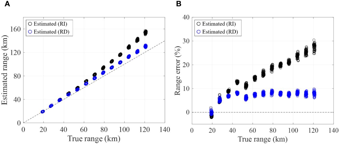
Figure 7 (A) Comparison of source-receiver distances measured by GPS (black dashed line) with distances estimated in range-independent bathymetry (black open circles) and distances estimated in range-dependent bathymetry (blue open circles). (B) Corresponding distance errors.

3.2 Inversion in range-dependent environment

To mitigate the discrepancy in the range-independent environment, we employ an adiabatic approximation for model propagation in the range-dependent environment (Jensen, 2011; Bonnel et al., 2022). The modeled modal travel times, denoted as ${\widehat{t}}_m(f_n,\text{ X})$ in (Equation 5), are calculated by dividing the source-receiver distance into range-independent segments based on a 1-m change in water depth for the bottom bathymetry depicted in Figure 1C. The modal travel times for each segment are then summed using Equation 9

$\begin{array}{ll}{\widehat{t}}_m(f_n,\text{ X})={\displaystyle \sum _{i=1}^{N_r}}\frac{\Delta r_i}{v_m(r_i,f_n,\text{ X})}& (9)\end{array}$

Here $N_r$ is the total number of range segments, $\Delta r_i$ represents the range in the ith range segment, and $v_m(r_i,f_n,\text{ X})$ is the group velocity predictions of mode m as a function of frequency for the ith range segment.

Subsequently, the inversion process was reiterated for the source-receiver distance of 18.6 km, and the inversion results are presented in Table 2. The estimated geoacoustic parameters in the range-dependent environment exhibited consistency with those in the range-independent environment, falling within 95% HPD credible intervals, except for the thickness of the surficial sediment, estimated to be 5.3 m. the revised results indicate a surficial sediment layer with a thickness of approximately 5.3 m. The surficial sediment layer has an approximate sound speed of 1432.6 m/s and a density of about 1.41 g/cm³. The underlying basement exhibits a sound speed of approximately 1737.6 m/s and a density of approximately 1.87 g/cm³. Based on these optimal values, we now re-estimate the source-receiver distances to 121.5 km using the optimal values for the range-dependent environment. Consequently, as the source-receiver distance increased, the distance error−up to 30% in the range-independent environment was reduced to within 10%. It was assumed that the estimated geoacoustic parameters were independent of changes in water depth with distance, possibly explaining why the error could not be further reduced.

Table 2

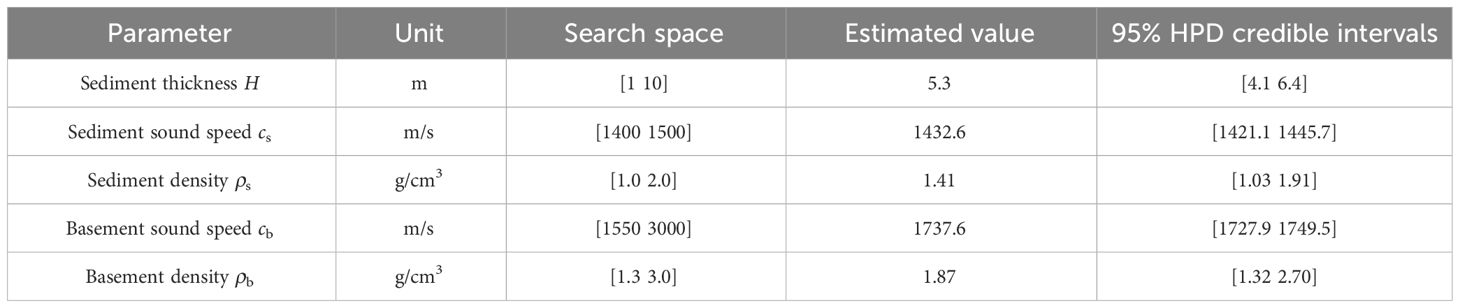
Table 2 Search spaces and estimated optimal parameter values for environmental parameters applied in geoacoustic inversion in the range-dependent environment.

4 Summary and conclusion

Over the past few years, our research has focused on the underwater acoustic environment of the East Siberian Shelf, a region that remains one of the least studied in the Arctic Ocean. In our initial paper (Han et al., 2021), we reported on the seasonal variations in ambient noise levels, revealing a strong negative correlation with changes in sea ice concentration covering the sea surface. In our subsequent paper (Han et al., 2023), we aimed to understand the acoustic propagation characteristics of the East Siberian Shelf. This involved analyzing seismic airgun sounds propagating over tens of kilometers and comparing them with the model predictions obtained from a broadband application of the range-dependent acoustic model (RAM). In this acoustic model, a two-layer geoacoustic bottom structure, presented in the previous references, was used as model input. Interestingly, modal dispersion was observed in the spectrogram of the signal propagating over several kilometers, and this observation served as the motivation for this paper.

In this paper, we tried to estimate the geoacoustic parameter values for the two-layer geoacoustic bottom model by comparing the dispersion curves extracted from the replicas predicted by the KRAKEN normal-mode program with dispersion curves extracted from the acoustic data for the source-receiver distance of 18.6 km. First, the inversion results, assuming a range-independent environment, revealed the best-fit values for the sediment sound speed and density in the surficial layer to be approximately 1422.4 m/s and 1.58 g/cm³, respectively. For the lower layer, these values were estimated to be 1733.6 m/s and 1.84 g/cm³, respectively and the surficial sediment thickness was estimated to be ~ 4.1 m. As mentioned in Section 1, previous studies have reported the presence of a soft, unconsolidated surficial sediment layer (less than 4 m thick) overlaying a glaciogenic overcompacted sediment layer (O’Regan et al., 2017; Jin, 2020). However, the surficial sediment parameters (H, c_s, ρ_s), including the basement density (ρ_b), exhibited limited sensitivity in predicting modal dispersion curves, as illustrated in Figure 5. This suggests that, within the frequency range of the airgun sound, the geoacoustic parameters of the soft surficial sediment may not significantly impact the modeling results.

Subsequently, the inversion results were applied to estimate source-receiver distances ranging from 18.6 to 121.5 km, employing the same method used for geoacoustic inversion. However, the estimated source-receiver distances exhibited increasing errors, reaching up to 30% as the distance increased. To mitigate the distance errors, we employed an adiabatic approximation for model propagation in the range-dependent environment. The modeled modal travel times were calculated by dividing the source-receiver distance into range-independent segments, each based on a 1-m change in water depth, and then summed. The inversion results demonstrated consistency with those obtained in the range-independent environment, except for the surficial sediment thickness, which was estimated to be ~ 5.3 m. Finally, the source-receiver distances were re-estimated using the geoacoustic parameters obtained under the range-dependent environment, resulting in a reduced distance error to within 10%. The simplification of sediment structure through a two-layer bottom geoacoustic model, as assumed in the study, might limit the accurate capture of depth variations relative to changes in sediment structure over distance. This limitation could contribute to the inability to further reduce distance error. Additionally, our study assumed the negligible shear wave effect on modal travel time, potentially posing another limitation in reducing distance errors. Potty and Miller (2020) reported that the impact of shear waves may intensify within the low-order mode Airy phase region, characterized by the minimum group velocity.

The estimation of the sediment attenuation coefficient was not undertaken in this study as this parameter does not influence modal travel time but rather affects modal amplitude. In Figure 6, it was observed that modes 3 and 4 are not distinctly visible in the measured spectrogram. The waveform, recorded by the near-field hydrophone, exhibited a spike-like signature, as depicted in Figure 3 of Han et al. (2023). The spectral peak of the airgun pulse was identified at approximately 27 Hz, beyond which the energy rapidly diminished, dropping to less than half around 100 Hz. Furthermore, the propagation of each mode is significantly influenced by the depth-dependent modal eigenfunctions. Figure 8 illustrates the depth-dependent modal eigenfunction for each mode at 100 Hz, within the frequency bands of mode 1–4. The modal amplitudes of modes 3 and 4, corresponding to the hydrophone depth, are smaller than those of modes 1 and 2. Lastly, the absence of ground truth data for comparison limits the ability to verify the reliability of the inversion results, given that the East Siberian Shelf is a poorly studied region. Despite these challenges, our inversion results hold value as they provide indirect information about the geoacoustic properties of the East Siberian Shelf.

Figure 8

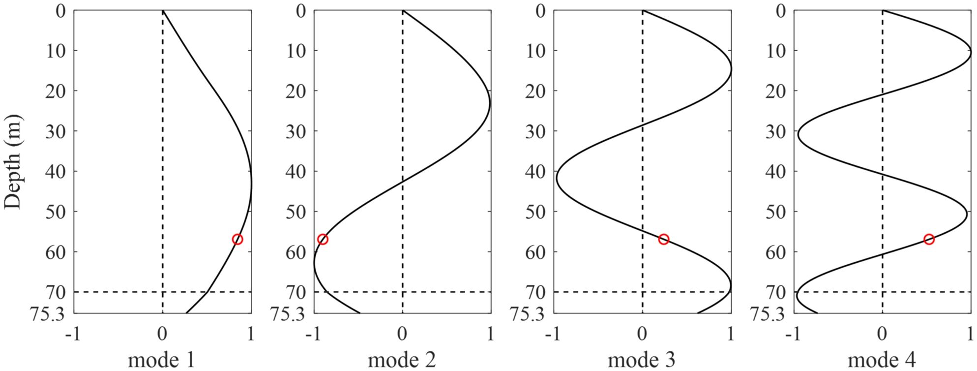
Figure 8 Depth-dependent modal eigenfunctions for modes 1–4 evaluated at 100 Hz. In each mode, the red circles represent modal eigenfunction amplitudes at the hydrophone depth.

Data availability statement

The original contributions presented in the study are included in the article/supplementary material. Further inquiries can be directed to the corresponding authors.

Author contributions

DL: Writing – review & editing, Writing – original draft, Methodology, Formal analysis, Data curation, Conceptualization. DH: Writing – original draft, Methodology, Data curation, Conceptualization. JC: Writing – review & editing, Writing – original draft, Validation, Supervision, Methodology, Funding acquisition, Formal analysis, Data curation, Conceptualization. WS: Writing – original draft, Investigation, Data curation, Conceptualization. EY: Writing – original draft, Investigation, Funding acquisition, Data curation, Conceptualization. HL: Writing – review & editing, Writing – original draft, Validation, Supervision, Methodology, Investigation, Funding acquisition, Formal analysis, Data curation, Conceptualization. DT: Writing – review & editing, Writing – original draft, Validation, Supervision, Methodology, Formal analysis.

Funding

The author(s) declare financial support was received for the research, authorship, and/or publication of this article. This research was supported by the Ministry of Oceans and Fisheries projects, entitled ‘Korea-Arctic Ocean Warming and Response of Ecosystem (20210605)’. This work was also supported by the National Research Foundation of Korea (NRF) grant funded by the Korea government (MSIT) (2020R1A2C2007772).

Conflict of interest

Author DH was employed by company Oceansounds Incorporation.

The remaining authors declare that the research was conducted in the absence of any commercial or financial relationships that could be construed as a potential conflict of interest.

Publisher’s note

All claims expressed in this article are solely those of the authors and do not necessarily represent those of their affiliated organizations, or those of the publisher, the editors and the reviewers. Any product that may be evaluated in this article, or claim that may be made by its manufacturer, is not guaranteed or endorsed by the publisher.

References

Ainslie M. (2010). Principles of sonar performance modelling (Berlin, Heidelberg: Springer Berlin Heidelberg: Imprint: Springer).

Google Scholar

Bonnel J., Chapman (2011). Geoacoustic inversion in a dispersive waveguide using warping operators. J. Acoust Soc. Am. 130, EL101–EL107. doi: 10.1121/1.3654580

PubMed Abstract | CrossRef Full Text | Google Scholar

Bonnel J., Dosso S. E., Chapman R. (2013). Bayesian geoacoustic inversion of single hydrophone light bulb data using warping dispersion analysis. J. Acoust Soc. Am. 134, 120–130. doi: 10.1121/1.4809678

PubMed Abstract | CrossRef Full Text | Google Scholar

Bonnel J., Dosso S. E., Goff J. A., Lin Y. T., Miller J. H., Potty G. R., et al. (2022). Transdimensional geoacoustic inversion using prior information on range-dependent seabed layering. IEEE J. Oceanic Eng. 47, 594–606. doi: 10.1109/JOE.2021.3062719

CrossRef Full Text | Google Scholar

Bonnel J., Thode A., Wright D., Chapman R. (2020). Nonlinear time-warping made simple: A step-by-step tutorial on underwater acoustic modal separation with a single hydrophone. J. Acoust Soc. Am. 147, 1897–1926. doi: 10.1121/10.0000937

PubMed Abstract | CrossRef Full Text | Google Scholar

Brown J., Ferrians O. J., Heginbottom J. A., Melnikov E. S. (1997). Circum-arctic map of permafrost and ground ice conditions (Washington, D. C: U. S. Geological Survey). Available at: https://web.archive.org/web/20170226114554id_/https://pubs.usgs.gov/cp/45/report.pdf.

Google Scholar

Choi J. W., Dahl P. H. (2007). Spectral properties of the interference head wave. J. Acoust Soc. Am. 122, 146–150. doi: 10.1121/1.2743156

PubMed Abstract | CrossRef Full Text | Google Scholar

Collins M. D. (1993). A split-step pade solution for the parabolic equation method. J. Acoust. Soc Am. 93, 1736–1742. doi: 10.1121/1.406739

CrossRef Full Text | Google Scholar

Conn A., Gould N., Toint P. (1997). A globally convergent Lagrangian barrier algorithm for optimization with general inequality constraints and simple bounds. Math. Comp. 66, 261–288. doi: 10.1090/S0025-5718-97-00777-1

CrossRef Full Text | Google Scholar

Dahl P. H., Choi J. W. (2006). Precursor arrivals in the Yellow Sea, their distinction from first-order head waves, and their geoacoustic inversion. J. Acoust Soc. Am. 120, 3525–3533. doi: 10.1121/1.2363938

PubMed Abstract | CrossRef Full Text | Google Scholar

Daubechies I., Lu J., Wu H.-T. (2011). Synchrosqueezed wavelet transforms: An empirical mode decomposition-like tool. Appl. Comput. Harmonic Anal. 30, 243–261. doi: 10.1016/j.acha.2010.08.002

CrossRef Full Text | Google Scholar

Dosso S. E. (2002). Quantifying uncertainty in geoacoustic inversion. I. A fast Gibbs sampler approach. J. Acoust Soc. Am. 111, 129–142. doi: 10.1121/1.1419086

PubMed Abstract | CrossRef Full Text | Google Scholar

Dosso S. E., Dettmer J. (2011). Bayesian matched-field geoacoustic inversion. Inverse Problems 27, 1–23. doi: 10.1088/0266-5611/27/5/055009

CrossRef Full Text | Google Scholar

Dove D., Polyak L., Coakley B. (2014). Widespread, multi-source glacial erosion on the chukchi margin, Arctic ocean. Quaternary Sci. Rev. 92, 112–122. doi: 10.1016/j.quascirev.2013.07.016

CrossRef Full Text | Google Scholar

Duan R., Chapman N. R., Yang K., Ma Y. (2016). Sequential inversion of modal data for sound attenuation in sediment at the New Jersey Shelf. J. Acoust. Soc Am. 139, 70–84. doi: 10.1121/1.4939122

PubMed Abstract | CrossRef Full Text | Google Scholar

Duarte C. M., Chapuis L., Collin S. P., Costa D. P., Devassy R. P., Eguiluz V. M., et al. (2021). The soundscape of the Anthropocene ocean. Science 371, 1–10. doi: 10.1126/science.aba4658

CrossRef Full Text | Google Scholar

Duncan A. J., Gavrilov A. N., McCauley R. D., Parnum I. M., Collis J. M. (2013). Characteristics of sound propagation in shallow water over an elastic seabed with a thin cap-rock layer. J. Acoust. Soc Am. 134, 207–215. doi: 10.1121/1.4809723

PubMed Abstract | CrossRef Full Text | Google Scholar

Frisk G. V. (1994). Ocean and seabed acoustics: a theory of wave propagation (Englewood Cliffs, N.J: PTR Prentice Hall).

Google Scholar

Frisk G. V. (2012). Noiseonomics: The relationship between ambient noise levels in the sea and global economic trends. Sci. Rep. 2, 437. doi: 10.1038/srep00437

PubMed Abstract | CrossRef Full Text | Google Scholar

Gelman A., Carlin J. B., Stern H. S., Dunson D. B., Vehtari A., Rubin D. B. (2013). Bayesian data analysis. 3rd ed (New York: Chapman and Hall/CRC). doi: 10.1201/b16018

CrossRef Full Text | Google Scholar

Gerstoft P., Mecklenbräuker C. F. (1998). Ocean acoustic inversion with estimation of a posteriori probability distributions. J. Acoust. Soc Am. 104, 808–819. doi: 10.1121/1.423355

CrossRef Full Text | Google Scholar

Goldberg D. E. (1989). Genetic algorithms in search, optimization and machine learning (Boston: Addison-Wesley).

Google Scholar

Han D.-G., Joo J., Son W., Cho K. H., Choi J. W., Yang E. J., et al. (2021). Effects of geophony and anthrophony on the underwater acoustic environment in the East Siberian Sea, Arctic ocean. Geophysical Res. Lett. 48, e2021GL093097. doi: 10.1029/2021GL093097

CrossRef Full Text | Google Scholar

Han D.-G., Kim S., Landrø M., Son W., Lee D. H., Yoon Y. G., et al. (2023). Seismic airgun sound propagation in shallow water of the East Siberian shelf and its prediction with the measured source signature. Front. Mar. Sci. 14. doi: 10.3389/fmars.2023.956323

CrossRef Full Text | Google Scholar

Hastings W. K. (1970). Monte carlo sampling methods using markov chains and their applications. Biometrika 57, 97–109. doi: 10.1093/biomet/57.1.97

CrossRef Full Text | Google Scholar

Iatsenko D., McClintock P. V. E., Stefanovska A. (2016). Extraction of instantaneous frequencies from ridges in time–frequency representations of signals. Signal Process. 125, 290–303. doi: 10.1016/j.sigpro.2016.01.024

CrossRef Full Text | Google Scholar

Jakobsson M., Mayer L. A., Bringensparr C., Castro C. F., Mohammad R., Johnson P., et al. (2020). The international bathymetric chart of the arctic ocean version 4.0. Sci. Data 7, 176. doi: 10.1038/s41597-020-0520-9

PubMed Abstract | CrossRef Full Text | Google Scholar

Jensen F. B. (2011). Computational ocean acoustics (New York: Springer). doi: 10.1007/978-1-4419-8678-8

CrossRef Full Text | Google Scholar

Jin Y. K. (2020) ARA10C cruise report: Korea- Russia East Siberian/Chukchi Sea research program. Available online at: http://library.kopri.re.kr/search/detail/CATTOT000000055761.

Google Scholar

Keen K. A., Thayre B. J., Hildebrand J. A., Wiggins S. M. (2018). Seismic airgun sound propagation in Arctic Ocean waveguides. Deep Sea Res. Part I: Oceanographic Res. Papers 141, 24–32. doi: 10.1016/j.dsr.2018.09.003

CrossRef Full Text | Google Scholar

Liu H., Yang K., Ma Y., Yang Q., Huang C. (2020). Synchrosqueezing transform for geoacoustic inversion with air-gun source in the East China Sea. Appl. Acoustics 169, 107460. doi: 10.1016/j.apacoust.2020.107460

CrossRef Full Text | Google Scholar

Mahanty M. M., Latha G., Venkatesan R., Ravichandran M., Atmanand M. A., Thirunavukarasu A., et al. (2020). Underwater sound to probe sea ice melting in the Arctic during winter. Sci. Rep. 10, 16047. doi: 10.1038/s41598-020-72917-4

PubMed Abstract | CrossRef Full Text | Google Scholar

Meignen S., Gardner T., Oberlin T. (2015). “Time-frequency ridge analysis based on the reassignment vector,” in 23rd European Signal Processing Conference (EUSIPCO): IEEE. 1486–1490.

Google Scholar

Metropolis N., Rosenbluth A. W., Rosenbluth M. N., Teller A. H., Teller E. (1953). Equation of state calculations by fast computing machines. J. Chem. Phys. 21, 1087–1092. doi: 10.1063/1.1699114

CrossRef Full Text | Google Scholar

Niessen F., Hong J. K., Hegewald A., Matthiessen J., Stein R., Kim H., et al. (2013). Repeated pleistocene glaciation of the East Siberian continental margin. Nat. Geosci. 6, 842–846. doi: 10.1038/ngeo1904

CrossRef Full Text | Google Scholar

O’Regan M., Backman J., Barrientos N., Cronin T. M., Gemery L., Kirchner N., et al. (2017). The de long trough: a newly discovered glacial trough on the East Siberian continental margin. Climate Past 13, 1269–1284. doi: 10.5194/cp-13-1269-2017

CrossRef Full Text | Google Scholar

Outridge P. M., Macdonald R. W., Wang F., Stern G. A., Dastoor A. P. (2008). A mass balance inventory of mercury in the Arctic Ocean. Environ. Chem. 5, 89–111. doi: 10.1071/EN08002

CrossRef Full Text | Google Scholar

Porter M. B. (1992). “The KRAKEN normal mode program” (Naval Research Lab Washington DC).

Google Scholar

Potty G. R., Miller J. H. (2020). Effect of shear on modal arrival times. IEEE J. Oceanic Eng. 45, 103–115. doi: 10.1109/JOE.48

CrossRef Full Text | Google Scholar

Romanovskii N. (2004). Permafrost of the east Siberian Arctic shelf and coastal lowlands. Quaternary Sci. Rev. 23, 1359–1369. doi: 10.1016/j.quascirev.2003.12.014

CrossRef Full Text | Google Scholar

Thakur G., Brevdo E., Fučkar N. S., Wu H.-T. (2013). The Synchrosqueezing algorithm for time-varying spectral analysis: Robustness properties and new paleoclimate applications. Signal Process. 93, 1079–1094. doi: 10.1016/j.sigpro.2012.11.029

CrossRef Full Text | Google Scholar

Thode A., Bonnel J., Thieury M., Fagan A., Verlinden C., Wright D., et al. (2017). Using nonlinear time warping to estimate North Pacific right whale calling depths in the Bering Sea. J. Acoust. Soc Am. 141, 3059–3069. doi: 10.1121/1.4982200

PubMed Abstract | CrossRef Full Text | Google Scholar

Warner G. A., Dosso S. E., Dettmer J., Hannay (2015). Bayesian environmental inversion of airgun modal dispersion using a single hydrophone in the Chukchi Sea. J. Acoust. Soc Am. 137, 3009–3023. doi: 10.1121/1.4921284

PubMed Abstract | CrossRef Full Text | Google Scholar

Warner G. A., Dosso S. E., Hannay D. E., Dettmer J. (2016). Bowhead whale localization using asynchronous hydrophones in the Chukchi Sea. J. Acoust. Soc Am. 140, 20–34. doi: 10.1121/1.4954755

PubMed Abstract | CrossRef Full Text | Google Scholar