Intraseasonal variability of the deep scattering layer induced by mesoscale eddy

The deep scattering layer (DSL), a stratum of the marine diel vertical migration (DVM) organisms inhabiting the mesopelagic ocean, plays a crucial role in transporting carbon and nutrients from the surface to depth through the migration of its organisms. Using 18 months of in-situ observations and altimeter sea level data, we reveal for the first time the intraseasonal variations and underlying mechanisms of the DSL and the DVM to the east of the Taiwan Island. Substantial vertical speeds acquired from the Acoustic Doppler Current Profiler were used to examine the distribution and variation of the DVM. Innovatively, the results for the power spectrum analysis of the scattering intensity demonstrated a significant intraseasonal variability (ISV) with an 80-day period in the DSL. Furthermore, the variation in the DVM was closely linked to the DSL and showed an 80-day ISV during the observation. A dynamic relationship between the ISV of the DSL east of Taiwan Island and the westward-propagating mesoscale eddies was established. Anticyclonic (cyclonic) eddy movement toward Taiwan Island triggers downward (upward) bending of the local isotherms, resulting in a layer of DSL warming (cooling) and subsequent upper boundary layer deepening (rising). These findings underscore the substantial influence of mesoscale eddies on biological activity in the mesopelagic ocean, establishing a novel understanding of ISV dynamics in the DSL and their links to eddy-induced processes.

1 Introduction

The deep scattering layer (DSL) is a ubiquitous acoustically dense layer in mesopelagic, and is a horizontally extensive and vertically narrow layer. The DSL serves as a prominent signature of marine organism distribution across the global ocean, typically situated at depths from 200 to 1,000 m, with a thickness of 50 to 200 m (Aksnes et al., 2017; David and Richard, 2018; Kaartvedt et al., 2019). The DSL exhibits its deepest distribution in the southern Indian Ocean and shallowest at the oxygen minimum zone in the eastern Pacific. Additionally, the majority of the migration organisms in the Western Pacific remain at a relatively wide depth range of 300–700 m (Klevjer et al., 2016). The depth of the DSL is mostly influenced by the dissolved oxygen concentration, integrated fluorescence, and average turbidity (Irigoien et al., 2014). The depth can be predicted from the primary productivity and surface wind stress (Proud et al., 2017). DSL organisms are important components of the marine food web. They feed on phytoplankton in the surface scattering layer (SSL) and serve as bait for larger animals (Turner, 2015). Moreover, DSL organisms significantly contribute to the transport of organic carbon during their daily migration; this transport is one of the main processes in the ‘‘biological pump’’ (Kozlow, 1995; Davison et al., 2013; Irigoien et al., 2014). Migration organisms induce the downward flux of particles, which include particulate organic carbon and calcium carbonate (Steinberg et al., 2012; Hansen and Visser, 2016). This migration-generated particle flux is equal to approximately 10–20% of the annual downward flux of particles in the North Pacific subtropical gyres (Ducklow et al., 2009).

The global DSL exhibits rich biodiversity, primarily comprising small mesopelagic fish, with a smaller proportion of cephalopods, crustaceans, and jellyfish (Barham, 1996; Yang et al., 1996; Zhang et al., 2018; Wang et al., 2019). A key feature for organisms comprising the DSL is that they inhabit the mesopelagic zone (200–1,000 m) in the day and the epipelagic zone (0–200 m) in the night (Church et al., 2013; Klevjer et al., 2016). The daily migration of mesopelagic organisms, known as diel vertical migration (DVM), constitutes the largest animal migration on Earth. Global estimates suggest that the mesopelagic organism biomass ranges from 1 to over 15 billion tons (McGillicuddy et al., 2007; Behrenfeld et al., 2019). However, not all mesopelagic residents migrate. Migration can also vary among species, individuals, life stages, regions, and seasons (Neilson and Perry, 1990; Cohen and Forward, 2016; Klevjer et al., 2016; Olivar et al., 2018). Previous studies have identified the major migrators as zooplankton and micronekton in the global oceans (Seki and Polovina, 2001; Judkins and Haedrich, 2018). In the South China Sea, the majority of Myctophiformes and the Perciformes undertake daily migration, while most Salmoniformes and Beryciformes remain in deep water during both the day and night (Catul et al., 2011; Wang et al., 2019).

Many observational methods disclosed the prevalence of DSL in the ocean. Various observational methods have documented the prevalence of the DSL in the ocean. These methods of the DSL and vertical organism migration observation include sampling or collection methods, in-situ observation methods, and tracking and simulation methods. Compared with collection, tracking, and simulation methods, in-situ observation methods typically use acoustic and optical techniques, which have low disruptivity and simple operation (Benoit-Bird and Lawson, 2016; Bandara et al., 2021). The acoustic technique is an approach of in-situ observation, providing observation data at high temporal and spatial resolutions. It has thus been widely applied in DSL studies (Johnson, 1948; Lv et al., 2007; Cisewski et al., 2010). The main types of acoustic equipment used at this stage include fish-finding echo sounders, fish and acoustic Doppler current profilers (ADCPs). Fish-finding echo sounders can aid in distinguishing particle sizes (Morán et al., 2022), while ADCPs can accurately identify velocity and trajectory. In previous methods, DVM trajectories were usually observed through ADCP echo intensity, in which the migration velocity is calculated based on the migration depth and time (Irigoien et al., 2014). However, vertical ADCP velocities can be used to directly observe the DVM velocities of organisms. This method is occasionally used in the long-term deployment of moored ADCPs (van Haren and Compton, 2013; Wang et al., 2014). Unfortunately, there has been negligible explorations on the period of the long-term DVM velocity.

DVM is usually caused by spatial and temporal changes in resources and risks, which balances the functions of food gathering and predator avoidance (Kaartvedt et al., 1996; Cresswell et al., 2011). Researches have indicated that the DVM of organisms is primarily controlled by ambient irradiance, as well as other influencing factors including temperature, food availability, and predation risk (Gehring and Rosbash, 2003; Gaten et al., 2008; Bandara et al., 2021). Furthermore, to explain the partial migration of migratory species, Bos et al. (2021) suggested that the DVM mechanism could be attributed to the Hunger-Satiation hypothesis. DVM typically occurs within the 20 min preceding sunrise and the 20 min following sunset, with a migration speed of approximately 6–8 cm/s, which correlates with the migration depth (Bianchi and Mislan, 2016).

Previous studies have indicated that mesoscale eddies can influence the biomass and distribution of upper-ocean organisms (Chen et al., 2015; Devine et al., 2021). Mesoscale eddies are characterized by currents that flow in a roughly circular motion around the center of the eddy. Eddies can transport nutrients, heat, salt, and biochemical tracers between different water masses (Doblin et al., 2016; Della et al., 2022). The physical processes of eddies increase plankton abundances and biological production in upwelling regions and along frontal zones (Chelton et al., 2011). It has been shown that mesoscale eddy pairs in the ocean generate submesoscale flows in response to geostrophic flows (Hu et al., 2023), and flows filament has also been observed at the edges of mesoscale eddies (Gula et al., 2014). These submesoscale filaments have led to chlorophyll-a filament within the eddies, including the enhancement of vertical nutrient transport, leading to increased primary productivity (Qiu et al., 2023). Changes in primary productivity are necessary for modifying the structure of biomass and vertical distribution. Additionally, the migrating biomass in eddies is different from that of surrounding waters, which leads to varying carbon fluxes inside and outside of the eddies (Yebra et al., 2005; Brannigan, 2016). However, core cyclonic eddies (CEs) and anticyclonic eddies (AEs) have different effects on organisms. CEs are usually characterized by high levels of primary productivity and plankton biomass due to nutrient upwelling in the core (Vaillancourt et al., 2003). Simultaneously, the cold core region of CEs is an aggregation zone for zooplankton and micronekton (Zimmerman and Biggs, 1999). In contrast, the core of AEs typically have a depressed permanent thermocline and become a biologically infertile area (Franks et al., 1986; Chen et al., 2015).

The subtropical Pacific Ocean is one of the world’s most active regions for mesoscale eddies (Qiu and Chen, 2010; Hiromichi et al., 2023). In the ocean to the east of Taiwan Island, where westward-propagating mesoscale eddies encounter the Kuroshio Current, the hydrodynamic environment is quite complex. Presently, research on the ecological effects of mesoscale eddies has largely focused on the mixed layer (Chelton et al., 2011), while investigations into the impact of mesoscale eddies on biological communities in the DSL remain relatively unexplored. Additionally, research on the DSL has mainly focused on daily and seasonal variations. For example, changes in the light period have led to a non-24-h period in DVM and DSL (Kim et al., 2016), while the DSL in the mid-latitudes is under the influence of the seasonal cycle of the ocean thermal structure, which shows significant seasonal variations (van Haren and Compton, 2013; Bandara et al., 2021). However, studies on the intraseasonal variability (ISV) of the DSL or the variability under the impact of sequential mesoscale eddies pale in comparison with studies focusing on daily and seasonal variations.

In this study, we first analyze the ISV character of the depth and intensity of the DSL and DVM based on in-situ mooring observations east of Taiwan Island. Our analysis shows that the ISV of the DSL and DVM is mainly influenced by westward-propagating mesoscale eddies. Mesoscale dynamic processes play an equally significant role in influencing the DSL and DVM. The remainder of this paper is organized as follows. The data and methodology are discussed in Section 2. Section 3 presents the observational results on the spatial-temporal characteristics of the DSL and DVM. Section 4 discusses the different effects of CEs and AEs on DSL variation. Section 5 summarizes our main findings.

2 Data and method

2.1 In-situ observations

A mooring system was deployed at 23° N, 122° E (Figure 1A) from January 2016 to May 2017 to observe the interaction between mesoscale eddies and the Kuroshio Current. The depth of the mooring system was approximately 4,900 m. Two acoustic ADCPs (75 kHz transducers fixed at a mooring of 350 m, one facing up and one facing down) collected acoustic and current data from the sea surface to 800 m. The vertical profiles consisted of hourly measurements with a vertical resolution of 8 m in 70 bins. The two ADCPs were installed back-to-back, with the installation structure shown in Figure 1B. There was a 17 m blank zone on the first layer closest to the ADCP. Section 2.3 describes the method for converting the echo intensity into scattered matter in water to remove power attenuation caused by propagation losses and some environmental and equipment-characteristic effects. Strict quality controls were applied to the data. Retained data needs to satisfy the following criteria. Current speeds and echo intensity variations should be anomaly-free and reasonable (current speeds ranging from –2 to +2 m/s; echo intensity > 40 counts). The data goodness rate (Percent Good) needs to be 70%, and the roll and pitch angles need to be less than 15°. After quality control and interpolation, the echo intensity and vertical velocity at 23°N, 122°E were obtained to observe the organism migration process.

Figure 1

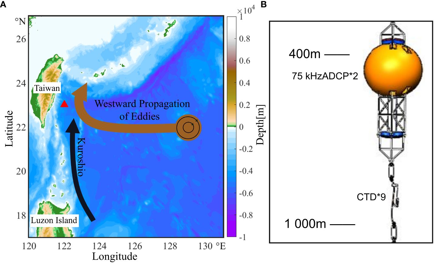
Figure 1 (A) Topographic map (depth; shading; unit: m) east of Taiwan Island derived from the Global Ocean Multi-Observation Products (https://marine.copernicus.eu/). The black arrow denotes the pathway of the Kuroshio Current and the brown arrow denotes the pathway of mesoscale eddies in the Kuroshio extension region. From January 2016 to May 2017, a mooring was located at 122° E, 23° N (green triangle), where water depth is approximately 4,900 m). (B) The 1,000 m mooring structure.

Temperature and salinity were measured using conductivity temperature depth (CTD) sensors. The CTD sensors were deployed between 400 and 1,000 m every 100 m on the mooring. Under the impact of vertical ocean currents, the CTD sensors and ADCP-equipped floating body were pressed down and vibrated (Wang et al., 2018). To ensure data quality, the depth vibration of the ADCP itself was removed with pressure data from the CTD sensor deployed at the same depth with the ADCP. The fluctuation speed of the ADCP ranged from –0.01 to 0.01 m/s. The vertical velocity at the ADCP was obtained after subtracting the speed fluctuations of the ADCP. The ADCP-equipped floating body was pressed down by 100–200 m when the mesoscale eddies passed by the mooring. The circulation of mesoscale eddies and velocity variation in the Kuroshio Current influenced by the mesoscale eddies induced the pressing depth. These vibrations resulted in the loss of some surface data, which did not influence the results of this study.

2.2 Satellite altimeter data

The dataset from Archiving, Validation, and Interpretation of Satellite Data in Oceanography (AVISO) was used and processed to investigate the effect of mesoscale eddies on the ISV of the DSL. Geostrophic velocity anomalies and sea level anomalies (SLAs) were obtained from the AVISO product Global ARMOR3D L4 reprocessed dataset (http://marine.copernicus.eu/services-portfolio/access-to-products/). The daily satellite data from January 2016 to May 2017 from 115°–145° E and 10°–35° N were extracted, with a horizontal resolution of 0.25° × 0.25°.

2.3 Calculation of acoustic scattering intensity

Based on the ADCP data, the biological distribution can be assessed by calculating the acoustic scatter strength (S_v), which was used to determine the existence of the DSL (RDI, 1996; Maclennan et al., 2002; Mullison, 2017):

$\begin{array}{ll}\begin{array}{c}{S}_v=C+10 \text{lg} [(T_x+273.16)R^2]-L_{DBM}-P_{DBW}\\ +2\alpha R+10 \text{lg} ({10}^{K_C(E-E_r)/10}-1)\end{array}& (1)\end{array}$

The parameters are based on the technical specifications for the 75 kHz ADCP provided in Deines (1999) and Mullison (2017). Here, C (= –163.3 dB) is the built-in system constant, including transducer and noise features, T_x is the real-time transducer position temperature (°C), R (= D/cosβ) is the range along the beam (slant range) to the scatterers (m), D is the depth cell length (m), and β (= 20°) is the beam angle from the system. Furthermore, L_DBM is 10lgL, where L (= ADCP transmit pulse time × sound speed) is the transmitted pulse length (m), P_DBW is 10lgP, where P (= 23.8 W) is the transmitted power (W), E is the echo intensity (count) returned by the ADCPs, E_r is the received signal strength indicator value when no signal is present (typically 40 counts), K_c (= 0.45 dB/LSB) is a conversion factor for the ADCP returned signal strength indicator slope (used to ensure that the expected error in S_v is ± 3 dB), and K_c and E_r are measured and recorded as part of factory testing. Finally, α is the sound absorption coefficient of water (dB/m), as determined by the frequency, depth, temperature, salinity, and acidity (Yang et al., 2019), calculated as Equation (2):

$\begin{array}{ll}\begin{array}{c}\alpha =0.106\frac{f_1{f}^2}{f^2+f_1^2}{e}^{\frac{pH-8}{0.56}}+0.52\left(1+\frac{T}{43}\right)\left(\frac{S}{35}\right)\frac{f_2{f}^2}{f^2+f_2^2}{e}^{-}\frac{z}{6}\\ +0.00049 f^2{e}^{-\left(\frac{T}{27}+\frac{z}{17}\right)}\end{array}& (2)\end{array}$

$f_1=0.78{(S/35)}^{1/2}{e}^{T/26}$ (for boron), and $f_1=42e^{T/17}$ (for magnesium).

Where S is the salinity of sea water (PSU), T is the temperature of sea water (°C), z is depth (km), and f denotes the sound frequency (kHz). In this study, the seawater salinity and temperature were observed by the CTD from 400–1,000 m. The salinity and temperature from 0–400 m were inverted and compared with the HYbrid Coordinate Ocean Model (HYCOM) assimilation data from the Naval Research Laboratory from January 2016 to May 2017. The assimilation data were used to study the vertical profile of the salinity and temperature at 23° N, 122° E east of Taiwan, China. The acidity was set at the default value of pH = 8 (Yang et al., 2019).

However, some areas of extremely anomalous scattering intensity were found based on the results calculated with Equation (1). The abnormally low values were found in the upper and lower 100 m interval of the ADCP depth, whereas the abnormally high values were found below 700 m. To avoid the occurrence of abnormally low values, we adjusted the abnormal interval by comparing different ADCP depths. All positions less than no signal (40 counts) were removed to avoid abnormally high values below 700 m.

3 Spatial and temporal characteristics of the DSL and DVM

3.1 Distribution of the observed DSL and DVM

Figure 2A shows the time–depth section of the daily S_v at 23°N, 122° E from January 2016 to June 2017. Figure 2 specifically shows the S_v values from 50 to 800 m, elucidating the strong scattering zone in the surface layer, presumably due to the presence of substantial bubble concentrations. There were two scattering layers detected during the observation: the upper layer, referred to as the SSL, and the bottom layer, referred to as the DSL.

Figure 2

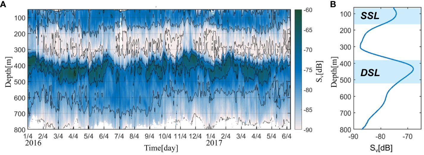
Figure 2 (A) Time–depth plot of the observed acoustic scattering intensity (S_v; unit: dB) east of Taiwan Island (23° N, 122° E) from January 2016 to June 2017. The black line represents the isogradient line (10 dB). (B) Vertical profile of the temporally averaged S_v during the observational period.

To examine the depth variation in the DSL and SSL, the maximum depth and boundary depth were calculated (Cisewski et al., 2021). Please refer to the appendix for details on the calculation method (Equations 3, 4). The upper boundary depth (lower boundary depth) of the SSL was in the 50–150 m (100–200 m) layer; the upper boundary depth (lower boundary depth) of the DSL was in the 300–450 m (400–550 m) layer. The SSL was observed in the 60–180 m, near the chlorophyll maximum layer, showing a mean intensity of –82 to –74 dB (Figure 2B). The DSL was in the 380–520 m layer in the mesopelagic zone, with a mean intensity ranging from –82 to –69 dB.

The DVM process could be measured based on the variation in the S_v between the SSL and DSL (Zhou et al., 1994). The vertical speeds were strong when the DVM was active between the SSL and DSL (Figures 3A, B). The range of speed in the vertical ocean current was generally within 10^–4 to 10^-5 m/s and the vertical current velocity was barely measurable by the ADCP (Pilo et al., 2018). The vertical speed acquired from the ADCP was approximately 0.1 m/s, which is significantly larger than that of the vertical current velocity. In the mesopelagic ocean, the vertical speeds measured by ADCPs cannot be regarded as the vertical current velocity, but rather represent the vertical speed associated with the DVM caused by organisms (Cisewski et al., 2021; Liu et al., 2022). Additionally, variations in the vertical speed corresponded with the S_v. As a result, the ADCP-measured vertical speeds were used to describe the variation in the DVM in this study.

Figure 3

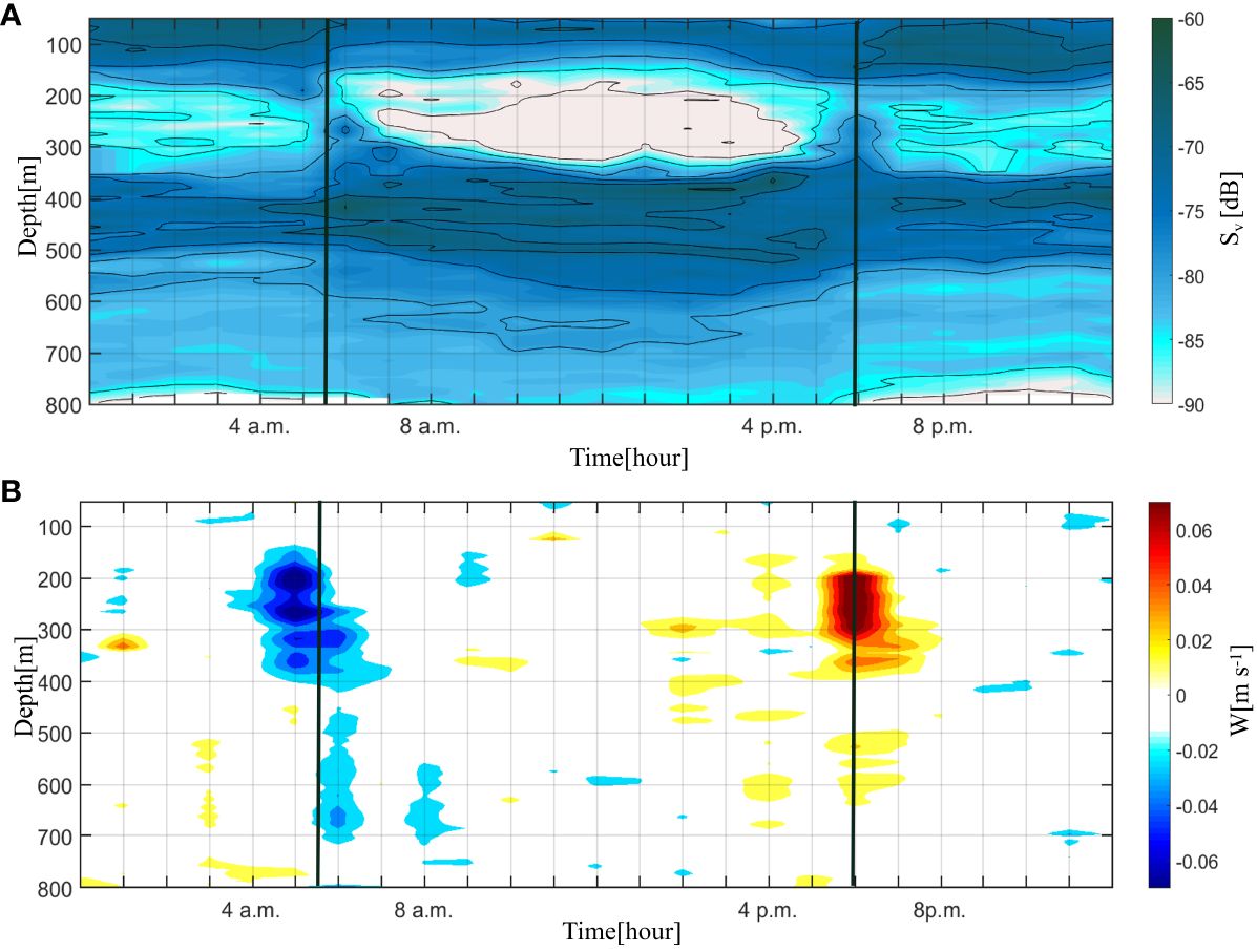
Figure 3 Time–depth plots of the (A) acoustic scattering intensity (S_v; unit: dB) and (B) vertical speed (W; unit: ms^–1) observed by the mooring on September 13, 2016. Positive values represent upward velocity and vice versa. Sunrise at 5:38 and sunset at 17:58 on September 23, 2016, as indicated by the black line.

Figures 3A, B shows that the S_v and vertical speed appear to have the same diurnal variation. The local sunrise and sunset times on that day were 5:38 and 17:58. According to Figure 3A, strong vertical migration occurred during the sunrise (4–8 a.m., UTC + 8) and sunset periods (4–8 p.m., UTC + 8), corresponding to S_v strengthening in the 200–400 m layer during those two periods. Generally, the Sv at night (8 p.m. to 4 a.m., UTC + 8) in the 200–400 m layer was 5–10 dB stronger than that during the day (8 a.m. to 4 p.m., UTC + 8), indicating higher biomass during the night, to the east of Taiwan Island. The vertical speed, representing the direction of the DVM, varied regularly in the 200–400 m layer during the day. The vertical speed was negative from 200–400 m 20 min before sunrise, with a magnitude of –0.02 to –0.08 m/s, corresponding to the downward phase of DVM. The DVM became upward at sunset; therefore, the vertical speed was positive from 200–400 m, ranging from 0.02 to 0.07 m/s. This indicates that organisms in the SSL respond to light earlier than organisms in the DSL.

The migration speed of the DVM can be confirmed by the S_v and vertical speed, indicating that organisms migrated between the DSL and SSL within the observation area. The DSL depth is controlled by the variable primary productivity, temperature, and dissolved oxygen (Bandara et al., 2021). The chlorophyll maximum exists in the 100–200 m layer in the western Pacific Ocean (Ding et al., 2022), which represents the optimal range for DVM organism predation. Consequently, these observation results could describe the DSL distribution and DVM process.

3.2 Intraseasonal variability in the observed DSL

The results of the power spectrum density (PSD) analysis (p< 0.05) showed two predominant periods of S_v. One was 24-h and the other was approximately 80 days, indicating diurnal and intraseasonal variations, respectively. The 24-h signal, as shown in Supplementary Figure S1, was the daily period caused by the DVM process. Returning to the mooring data (Figure 3), the migration trajectory and proportion were inferred from the S_v results. The direction and magnitude of the migration speed were justified by the vertical speed.

The 80-day period signal was significant in the upper boundary depth and lower boundary depth of the DSL (Figure 4A), indicating that DSL exhibited ISV during our observations. The S_v was thus filtered by a 20–90-day bandpass filter to further investigate the ISV of the DSL. As shown in Figure 4B, the S_v varied regularly with the ISV signal, especially in the DSL. Figure 4B indicates a notable 2–3 months distribution of a peak S_v. This peak was strongest both at the upper boundary depth and lower boundary depth of the DSL, indicating active migration of organisms in these layers. The intensity anomalies of upper and lower boundary depths were out of phase. Combined with Figure 2, this opposite phase indicates that the ISV of the DSL showed an overall increase and decrease in the DSL between 350 and 500 m.When the DSL is depressed, the Sv at the upper boundary location is weakened and the Sv at the lower boundary is enhanced, and vice versa. This period of weakening and strengthening is 80-days.

Figure 4

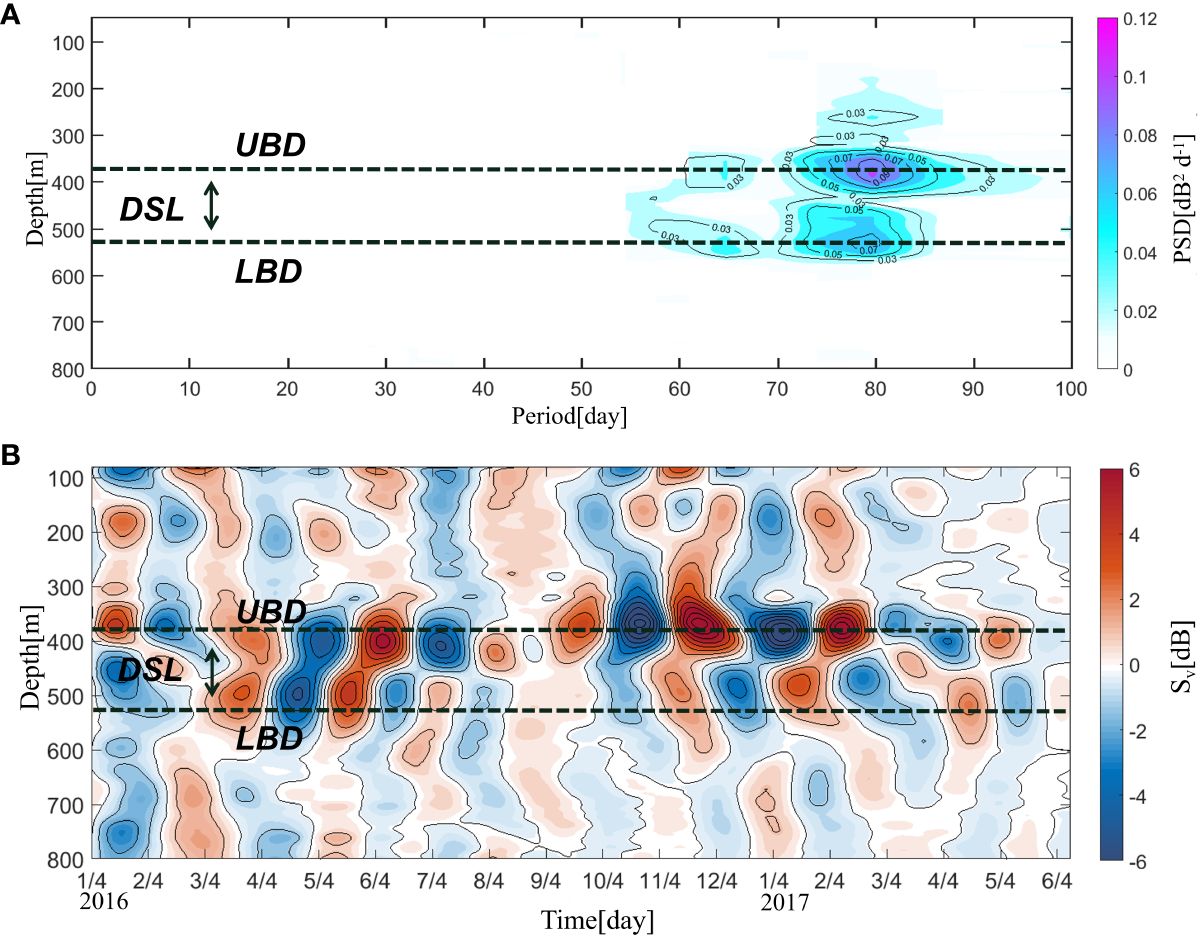
Figure 4 (A) Power spectrum density (PSD) of the acoustic scattering intensity (unit: dB² d^–1) from 0 to 100 days in the 50–800 m layer (95% confidence level). (B) Time–depth plot of the acoustic scattering intensity (S_v; unit: dB; 20–90-day band-pass filtered) anomaly. The black-dashed lines indicate the upper boundary depth (UBD) and lower boundary depth (LBD) of the deep scattering layer (DSL).

3.3 Intraseasonal variability in the observed DVM

Figures 5A, B shows the daily speeds in the downward and upward DVM between the SSL and DSL. The downward (upward) speed was the average speed during the sunrise (sunset) period. Figures 5C, D shows the temporal average of the vertical speeds during the observation. Unlike the vertical speed of the upward DVM, the speed of the downward DVM remained strong in the 250–350 m layer; therefore, the average downward speed of the DVM (–0.068 m/s) was stronger than the average upward speed of the DVM (0.045 m/s). This result agrees with previous studies, in which the speed of the DVM was calculated from the S_v, but not from observed vertical speeds (Bianchi and Mislan, 2016).

Figure 5

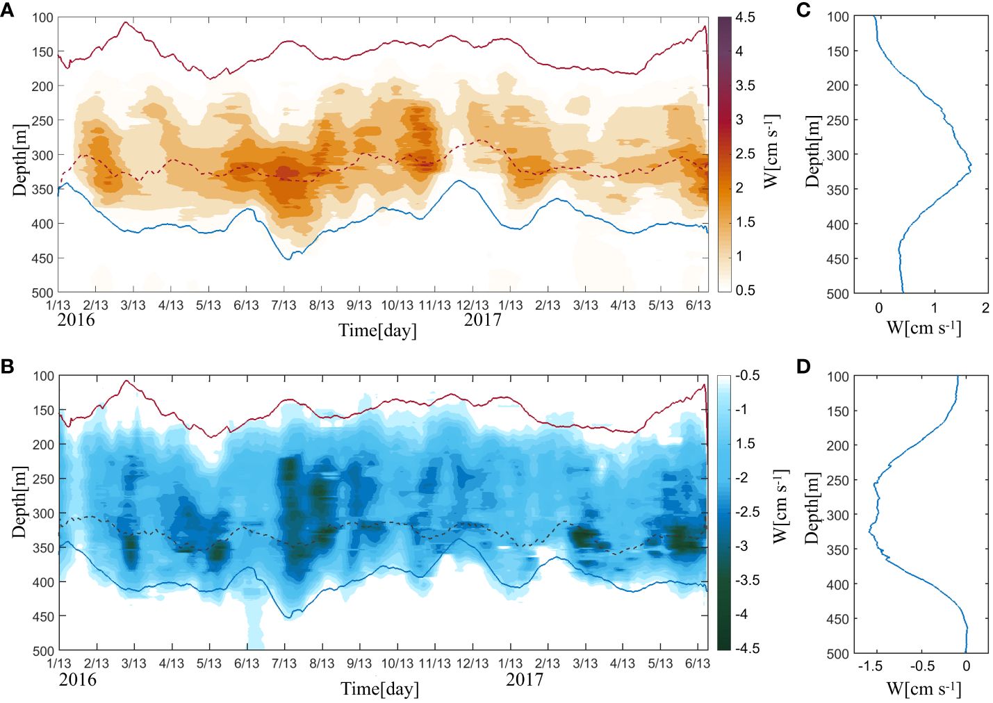
Figure 5 Time–depth plots of the observed daily (A) upward and (B) downward speeds (W; unit: cm s^–1; 20-day low-pass filtered). The solid red and blue lines in a) and b) represent the lower boundary of the SSL and upper boundary of the DSL, respectively. The red (purple)-dashed line in (A, B) indicates the maximum upward (downward) speed line. Temporal average of the (C) upward and (D) downward speeds calculated during the observation period.

To investigate the relationship between variations in the DVM and the scattering layers, correlation coefficients for the start (end) position of the DVM with the lower boundary depth of the SSL (red line in Figure 5) and the upper boundary depth of the DSL (blue line in Figure 5) were calculated. The boundaries of the DVM were defined as the depths where the vertical speed was 0.01 m/s (–0.01 m/s) in the upward (downward) DVM process. During the upward process, the upper boundary depth (lower boundary depth) of the DVM represented the position where organisms approximately began (stopped) upward migration. During the downward process, the lower boundary depth (upper boundary depth) of the DVM was the position where organisms began (stopped) downward migration. The upper boundary depth of the DSL showed a strong correlation with both the lower boundary depth of the upward DVM (n = 518, r = 0.82, and p< 0.05) and the lower boundary depth of the downward DVM (n = 518, r = 0.80, and p< 0.05). However, the lower boundary depth of the SSL showed a relatively weak correlation with both the upper boundary depth of the upward DVM (n = 518, r = 0.31, and p< 0.05) and the upper boundary depth of the downward DVM (n = 518, r = 0.61, and p< 0.05). The boundaries of the DVM were the positions of organisms moving in and out of the dense habitat, i.e., the DSL and SSL. Variations in the DSL and SSL thus led to variations in the boundaries of the DVM. During the sunset period, when the DSL rises (deepens), organisms from the DSL move out of the upper boundary depth at a higher (lower) depth; organisms begin upward migration at a higher (lower) depth. During the sunrise period, the starting point of the downward DVM changes in accordance with the lower boundary depth of the SSL, where organisms move out from that layer. Due to the higher speed of the downward DVM, organisms moving from the SSL would stop moving near the upper boundary depth of the DSL (Figure 5B); therefore, the lower boundary depth of the DVM was also well correlated with the upper boundary depth of the DSL. Numerous studies have indicated that the environment in which the SSL is located may be affected by various factors, such as temperature, wind, waves, and currents (Rykaczewski and Checkley, 2008; Sunday et al., 2012; Morioka et al., 2019). Furthermore, the speed of the DVM at the lower boundary of the SSL significantly decreased. In contrast, the mesopelagic zone (i.e., location of the DSL) was relatively stable; the period of the S_v in the DSL layer was notable and single. The variation in the lower boundary depth of the DVM was dominated by the DSL.

As the vertical range of the DVM was affected by the variation in the DSL, the PSD analysis was applied to detect the variation in the upward and downward speeds of the DVM below 50 m (Figure 6). The ISV signals of the upward and downward DVM were found at a depth of 50 m above the upper boundary depth of the DSL (average depth of approximately 394.3 m). The strongest signal was at approximately 350 m at the location of the maximum DVM speeds (dashed lines in Figures 5A, B). The mean depths of the maximum speeds in the upward and downward DVM were 317.2 and 330.7 m, respectively. The upper boundary depth of the DSL exhibited a good correlation with both the maximum speed depth of the upward DVM (n = 518, r = 0.60) and downward DVM (n = 518, r = 0.62). The location of the maximum speed was influenced by the variation in the upper boundary depth of the DSL; hence, the DVM speeds also exhibited a significant ISV signal.

Figure 6

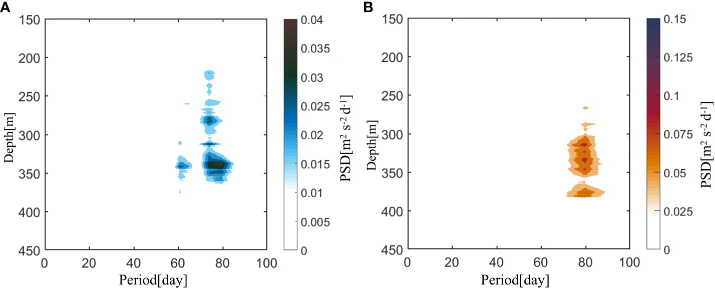
Figure 6 Power spectrum densities (PSD) of (A) downward and (B) upward velocities (unit: m 2 s^-2 d^-1) display from 150 m to 450 m (95% confidence level).

4 Effect of mesoscale eddies on the ISV of DSL

Mesoscale eddies have considerable impacts on the ISV of hydrological elements east of Taiwan Island (Zhang et al., 2001; Gilson and Roemmich, 2002; Liu and Li, 2013; Mensah et al., 2015). As this study focuses on the DSL east of Taiwan Island, we investigated the effects of mesoscale eddies on the DSL. Figure 7 shows that the SLA at 23°N, 122°E exhibits a significant ISV with an 83.5 days period (p< 0.05), which is consistent with the ISV of the DSL. This indicates that the ISV of the DSL is related to mesoscale eddy activity. Figure 8 shows the correlation coefficients of the time-lagged correlation between the S_v above 800 m and the SLA at 23°N, 122°E. The strongest positive (negative) correlation appeared at the lower boundary depth (upper boundary depth) of the DSL. A negative correlation between the S_v at the upper boundary depth of the DSL and the SLA was the largest when the SLA changed 10 days in advance (r = –0.68, p< 0.05). The strongest positive correlation appeared at the lower boundary depth of the DSL when the S_v changed 23 days later than that of the SLA (r = 0.49, p< 0.05).

Figure 7

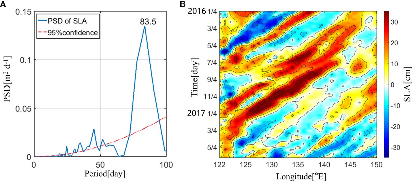
Figure 7 (A) Power spectrum densities (PSD) of the sea level anomaly (SLA; unit: m² d^-1) at 122°E, 23°N. The red-dotted indicates 95% confidence level. (B) Time-longitude plots of the SLA along the 23°N section from January 2016 to May 2017.

Figure 8

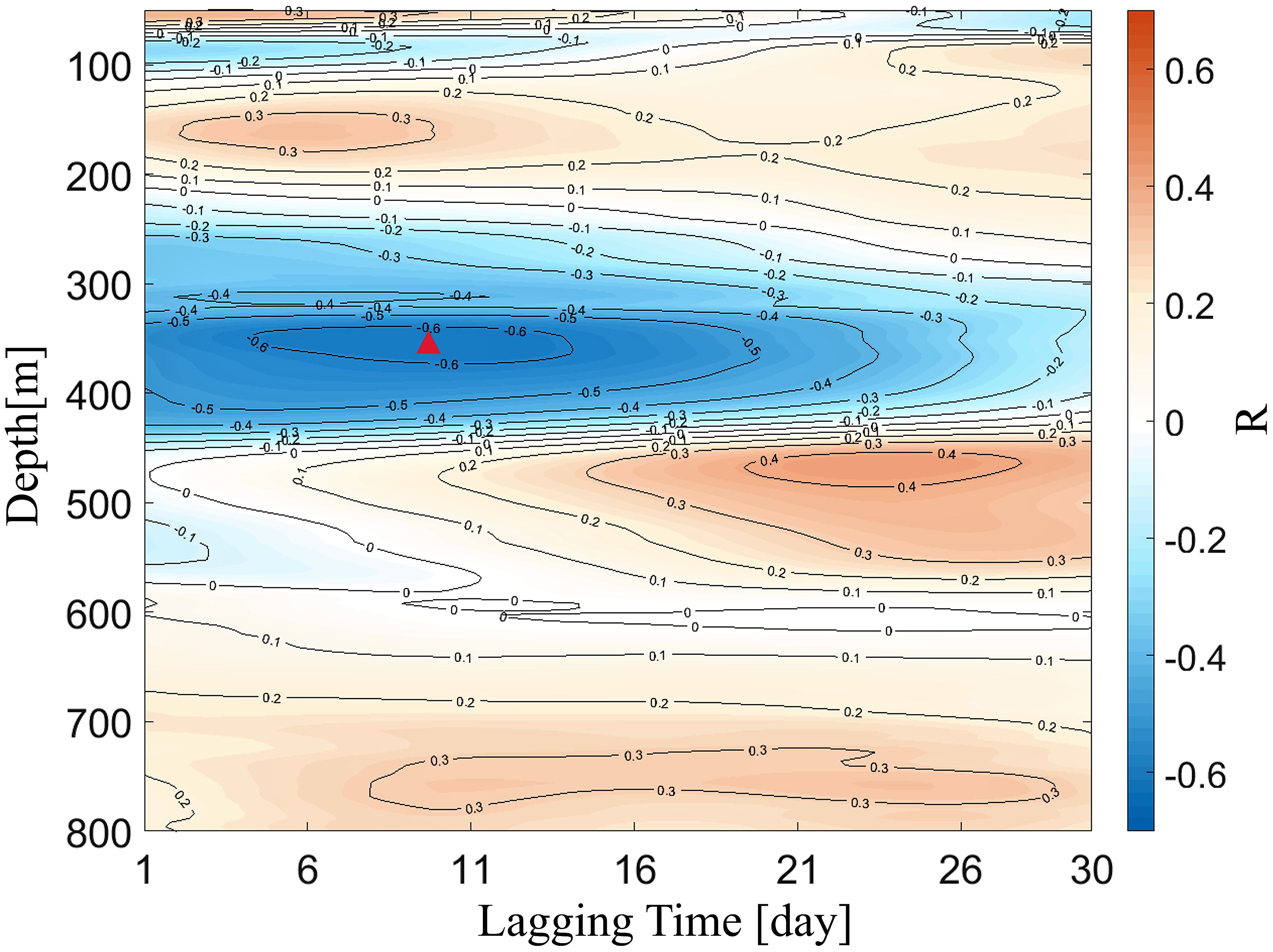
Figure 8 Results of time-lagged correlation (95% confidence level) between the sea level anomaly (SLA; unit: cm) and acoustic scattering intensity (S_v; unit: dB). The red triangle denotes is the point of the strongest correlation. Positive lagging time indicates the S_v lags the SLA.

As is shown in Figures 9A, B, the upper boundary depth anomaly of the DSL has a significant negative correlation with the SLA, with a correlation coefficient reaching –0.63. The Sv anomaly at the upper boundary depth of the DSL was also significantly correlated with the SLA, with a correlation coefficient of –0.58. The correlation of the SLA with the upper boundary depth of the Sv was stronger during the eddy periods than that during non-eddy periods. During eddy periods, the correlation coefficients of the SLA with the upper boundary depth and Sv at the upper boundary depth reached 0.67 and 0.62 (p< 0.05), respectively. In contrast, the correlation coefficients of the SLA with the upper boundary depth and Sv at the upper boundary depth were only 0.21 and 0.26 (p< 0.05), respectively, during non-eddy periods. As a result, the appearance of mesoscale eddies will cause noticeable changes in the DSL; this can be traced back to the modifications that eddies have on the local ecology (McGillicuddy, 2015).

Figure 9

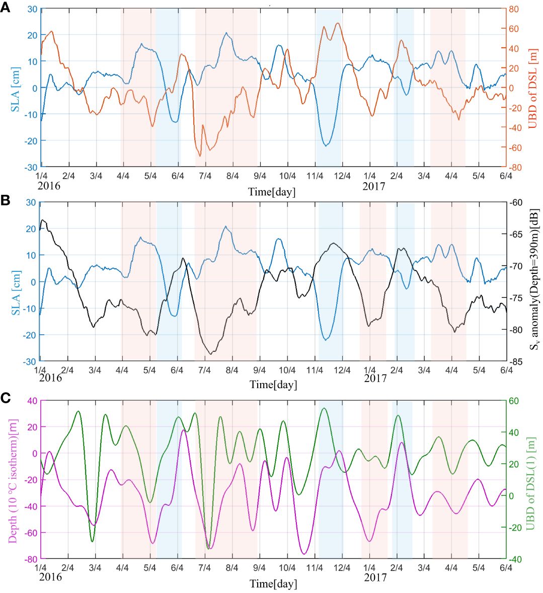
Figure 9 Time-series (January 2016 to May 2017) of the anomalies of the (A) daily upper boundary depth (UBD) in the deep scattering layer (DSL; red) and sea level anomaly (SLA; blue)with a 10-day lag, (B) DSL intensity of the upper boundary depth (black) and SLA (blue)with a 10-day lag, (C) depth of the 10°C isot+herm (purple; 20–90-day band-pass filtered) and upper boundary depth (magenta; 20–90-day band-pass filtered). The red and blue areas indicate the periods during which anticyclone and cyclone eddies occurred (n = 185).

Changes in the DSL are controlled by the variation in the dissolved oxygen (Klevjer et al., 2016; Liu et al., 2022). Variations in the dissolved oxygen are highly correlated with the oceanic temperature (Deutsch et al., 2005; Mavropoulou et al., 2020); both of them show corresponding changes under the effects of eddies (Kouketsu et al., 2016; Ren et al., 2020, 2022). The isotherm was calculated based on linear interpolation across the CTD sensors deployed every 100 m. Figure 9C shows the variation in the 10°C isotherm depth in the mesopelagic ocean and the upper boundary depth after 20–90-day bandpass filtering. The 10°C isotherm depth changed in accordance with the upper boundary depth (r = 0.56, p< 0.05), indicating that temperature is an important predictor of DSL variation, which agrees with Proud et al. (2017). Therefore, although dissolved oxygen data are not available in this in-situ observation, temperature was used to investigate the dynamic of eddy effects on the DSL in this study.

Figure 10A shows four cases of two AEs and two CEs arriving east of Taiwan Island. Figure 10B is the corresponding process temperature variation. Figure 10C shows the upper boundary depth variation in the DSL during these four cases. As shown in Figures 10B, C, the arrival of eddies leads to variations in the vertical structures of the temperature in the 400–600 m layer; thus, the DSL changes east of Taiwan Island. As AEs move toward Taiwan Island, the upper boundary depth of the DSL gradually deepens when the isotherms bend downward, resulting in warming in the 400–600 m layer: a warm environment favors organisms that live in the deep ocean (Proud et al., 2017). Conversely, CEs cause the bending upward of isotherms and thus cooling of the 400–600 m layer. The cooling condition is unfavorable to organisms migrating in the DSL, thereby promoting an increase in the upper boundary depth of the DSL. Consequently, there is stronger variation in the DSL during the eddy-period than that of the non-eddy period. The DSL exhibited a significant ISV, which agrees with the predominant variability in the eddy activity.

Figure 10

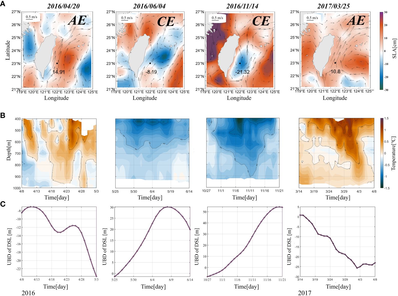
Figure 10 Distributions of the (A) sea level anomaly (SLA; shading; unit: cm) and sea surface current (black arrows) during cases when mesoscale eddies occurred to the east of Taiwan Island. Anticyclonic eddies occurred on April 20, 2016, and November 14, 2016, while cyclonic eddies occurred on June 4, 2016, and January 6, 2017. The numbers in a) are the sea surface height (m) at the location of mooring (black dots). (B) Time–depth plots of the temperature during the four cases with the passing of mesoscale eddies. (C) Time-series of the upper boundary depth of the DSL anomalies during four cases with the passing of mesoscale eddies passing. Time–depth plots in b) were measured via the CTD deployed at depths of 400–1 000 m.

5 Summary and discussion

Based on in-situ observations from January 2016 to May 2017 obtained east of Taiwan Island, we found a significant ISV in the DSL. Furthermore, vertical speeds from the ADCP were used to innovatively describe the process and variation in the DVM, while previous studies generally calculated the speed with the acoustics intensity and migration trajectory (Bianchi and Mislan, 2016). The mean speed of the downward DVM was stronger than that of the upward DVM, identical to previous studies (Bianchi and Mislan, 2016). As shown in Figure 11, the DVM occurred between the DSL and SSL, with strong downward and upward migration occurring during the sunrise (4–8 a.m., UTC + 8) and sunset periods (4–8 p.m., UTC + 8), respectively. During the sunrise (sunset) period, organisms move downward (upward) from the SSL (DSL). We also proved that the interval of the DVM corresponded with the variations in the upper boundary depth of the DSL and lower boundary depth of the SSL. The maximum speed depth and lower boundary depth of the DVM varied with the depth of the upper boundary depth of the DSL. In summary, we demonstrated that the upper boundary depth of the DSL plays a more important role in variations in the DVM; thus, the vertical speed of the DVM also exhibited notable ISV.

Figure 11

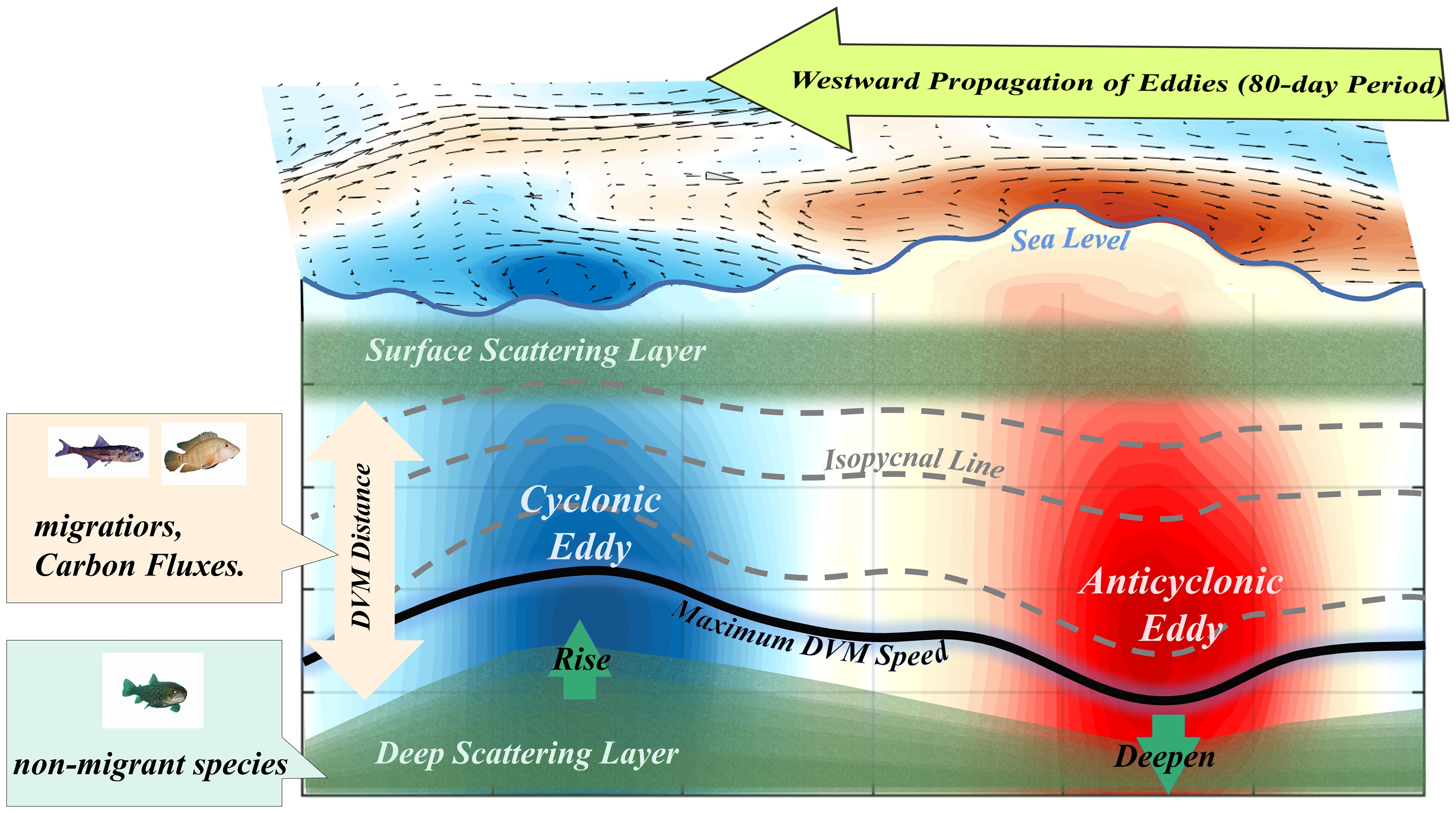
Figure 11 Intraseasonal variability (ISV) in the deep scattering layer (DSL). The westward propagation of mesoscale eddies causes temperature anomalies (shading) in the mesopelagic ocean, which are accompanied by ISV (80-day period) in the upper boundary depth of the DSL. With the passing of a CE, the mesopelagic ocean showed a negative temperature anomaly with an increase in the upper boundary depth of the DSL; an AE showed the opposite effect. The velocity distribution of DVM is closely related to the depth oscillation of the upper boundary depth of the DSL. The DVM distance of migrant species adjusts with the change in the upper boundary depth of the DSL. The position of the maximum DVM speed also shows an ISV with the change in the upper boundary depth of the DSL.

Mesoscale eddies occur frequently east of Taiwan Island, and the ISV of the DSL is related to mesoscale eddy activity. According to Figure 9, the DSL changes noticeably when there is mesoscale eddy arrival at the location of the ADCP. Xiu and Chai (2020) and Qiu et al. (2022) pointed out the negative and positive temperature anomalies in the mid-ocean of 200m-500m under the influence of cyclones and anticyclones, which fit the results of this paper. When the AEs move toward the ADCP location, isotherms bend downward, and the temperature increases in the 400–600 m layer. This warming condition is beneficial to the marine organisms moving out of the scattering layers, leading to a gradual deepening of the upper boundary depth of the DSL. In contrast, CEs cause decreases in the temperature in the 400–600 m layer, and this result is not beneficial to organisms migrating in the DSL; thus, there is an increase in the upper boundary depth of the DSL. DSL organism contains a very large number of nighttime non-migratory populations. This implies that the lower boundary of diurnal migration is the DSL, and that changes in the depth of the DSL are responsible for changes in diurnal migration distances.

The SSL and DSL are regarded as two habitats for DVM organisms; and their intensity are notably the strongest in the epipelagic and mesopelagic zones. Average data from all oceans suggest that the SSL has the strongest S_v in the 50–800 m layer (Irigoien et al., 2014). However, our data in the western Pacific shows that the intensity of the DSL is stronger than that of the SSL. The S_v of the DSL is also the strongest layer in 50–800 m layer of north Atlantic and east Pacific (Song et al., 2022). The difference in the S_v of the SSL and DSL at different areas may be caused by the vertical distribution of organism. Suboxic and hypoxic conditions occur in regions where the S_v SSL is weaker than that of the DSL (Keeling et al., 2010).

Eddies can change to the local carbon flux (Hernández-León et al., 2001; Yebra et al., 2005); the ISV of the depth and intensity in the DSL induced by eddies is the biological reason for the change in the carbon flux. The mooring observations could better show the time evolution of the hydrographic impact (especially eddies) on the DSL east of Taiwan Island. However, in previous observations, numerous shipboard ocean time-series provided data, such as the depth and intensity of the global DSL (Proud et al., 2017), which suggest that the depth and intensity of the DSL is variable in different areas. As a result, biological factors that induce the change in the carbon flux differ from region to region, but we are far from realistically quantifying them. Therefore, we must focus on local observations. For example, the particle size distribution of organisms can be measured via trawling, which can correct the S_v, followed by calculating the local biomass. Additionally, we can measure the export flux of particulate organic carbon in the local mesopelagic ocean, thus allowing further quantification of the relationship between the ISV and carbon cycle.

Overall, although some studies have found that the DSL has an important influence on the oceanic carbon cycle (Kozlow, 1995; Davison et al., 2013), the influence of multi timescale oceanic hydrology variations on the DSL remains underestimated. Our results demonstrated that mesoscale processes have an impact on DSL in the oceanic mesopelagic zone, but there is still a lack of local netting results to help us complete the composition of local DVM organisms. At the same time, quantifications of the influence of DVM organism life processes on the variation in DSL are also scarce. Therefore, more observation and biological activity research on DSL organism should be performed in future studies.

6 Appendix

Referring to Cisewski et al. (2021), the weighted mean depth of the backscatter was used to determine the mean depth of the DSL and SSL. The SSL and DSL were divided into two intervals by the 300 m layer. The weighted mean depths were both calculated for each S_v profile interval as follows:

$\begin{array}{ll}{\text{D}}_{\text{L}}={\sum }_{\text{i}=1}^{\text{N}}{\text{S}}_{\text{vi }}{\text{z}}_{\text{i}}/{\sum }_{\text{i}=1}^{\text{N}}{\text{S}}_{\text{vi }}& (3)\end{array}$

where D_L is the maximum depth of the SSL and DSL, S_vi is the volume backscattering intensity, and z_i is corresponding depths.

Further, to obtain the upper and lower boundaries of the SSL and DSL, the S_v was subjected to gradient analysis to obtain the upper and lower increasing and decreasing intervals of the SSL and DSL. Similarly, the weighted mean depth of the backscatter was used to determine the mean depth of the DSL and SSL boundaries. We divided the boundary region for the gradient analysis results of S_v into four intervals by three lines, which were the maximum depth of the DSL and SSL and the 300-m depth layer. From shallow to deep, each of the four intervals contained the upper and lower boundaries of the SSL and DSL. The weighted mean depths were calculated for each gradient analysis result of the S_v profile interval as follows:

$\begin{array}{ll}{\text{D}}_{\text{B}}={\sum }_{\text{i}=1}^{\text{N}}{\text{S}}_{\text{vgi }}{\text{z}}_{\text{i}}/{\sum }_{\text{i}=1}^{\text{N}}{\text{S}}_{\text{vgi }}& (4)\end{array}$

where D_B is the upper and lower boundary depths of the SSL and DSL, S_vgi is the volume gradient analysis result of the backscattering coefficient, and z_i is the corresponding depth.

Data availability statement

The original contributions presented in the study are included in the article/Supplementary Material. Further inquiries can be directed to the corresponding authors.

Author contributions

BW: Writing – original draft, Writing – review & editing, Conceptualization, Data curation, Formal analysis, Funding acquisition, Investigation, Methodology, Project administration, Resources, Software, Supervision, Validation, Visualization. FY: Writing – review & editing. RW: Methodology, Supervision, Writing – review & editing. ZT: Supervision, Writing – review & editing. QR: Funding acquisition, Methodology, Writing – review & editing. XL: Supervision, Writing – review & editing. JW: Supervision, Writing – review & editing.

Funding

The author(s) declare financial support was received for the research, authorship, and/or publication of this article. This work was supported by the national Natural Science Foundation of China (No. 42206032), the Science Foundation of Shandong Province (No. ZR2022QD045) and the National Key R,D Program of China (No.2022YFC3104100).

Acknowledgments

The authors wish to express their sincere gratitude to the crew of R/V Science as well as to all the scientists and technicians involved in the deployment and/or retrieval of the subsurface mooring that provided these valuable data. The provision of satellite data by AVISO is also greatly appreciated.

Conflict of interest

The authors declare that the research was conducted in the absence of any commercial or financial relationships that could be construed as a potential conflict of interest.

Publisher’s note

All claims expressed in this article are solely those of the authors and do not necessarily represent those of their affiliated organizations, or those of the publisher, the editors and the reviewers. Any product that may be evaluated in this article, or claim that may be made by its manufacturer, is not guaranteed or endorsed by the publisher.

Supplementary material

The Supplementary Material for this article can be found online at: https://www.frontiersin.org/articles/10.3389/fmars.2024.1367410/full#supplementary-material

Supplementary Figure 1 | Periods from 23 ~ 25 hours power spectrum density (unit: dB² d^-1) of acoustic scattering intensity in the 50 m ~ 800 m layer (95% confidence level).

Abbreviations

ADCP, Acoustic Doppler current profilers; AE, Anticyclonic eddy; AVISO, Archiving, Validation, and Interpretation of Satellite Data in Oceanography; CE, Cyclonic eddy; CTD, Conductivity temperature depth; DSL, Deep scattering layer; DVM, Diel vertical migration; HYCOM, HYbrid Coordinate Ocean Model; ISV, Intraseasonal variability; LBD, Lower boundary depth; PSD, Power spectrum density; SLA, Sea level anomaly; SSL, Surface scattering layer; UBD, Upper boundary depth.

References

Aksnes D. L., Rostad A., Kaartvedt S., Martinez U., Duarte C. M., Irigoien X. (2017). Light penetration structures the deep acoustic scattering layers in the global ocean. Sci. Adv. 3. doi: 10.1126/sciadv.1602468

CrossRef Full Text | Google Scholar

Bandara K., Varpe O., Wijewardene L., Tverberg V., Eiane K. (2021). Two hundred years of zooplankton vertical migration research. Biol. Rev. 96, 1547–1589. doi: 10.1111/brv.12715

CrossRef Full Text | Google Scholar

Barham E. G. (1996). Deep scattering layer migration and composition: observations from a diving saucer. Science 151(1966), 1399–1403. doi: 10.1126/science.151.3716.1399

CrossRef Full Text | Google Scholar

Behrenfeld M. J., Gaube P., Della Penna A. (2019). Global satellite-observed daily vertical migrations of ocean animals. Nature 576, 257–261. doi: 10.1038/s41586-019-1796-9

PubMed Abstract | CrossRef Full Text | Google Scholar

Benoit-Bird K. J., Lawson G. L. (2016). Ecological insights from pelagic habitats acquired using active acoustic techniques. Annu. Rev. Mar. Sci. 8, 463–490. doi: 10.1146/annurev-marine-122414-034001

CrossRef Full Text | Google Scholar

Bianchi D., Mislan K. A. S. (2016). Global patterns of diel vertical migration times and velocities from acoustic data. Limnology Oceanography 61, 353–364. doi: 10.1002/lno.10219

CrossRef Full Text | Google Scholar

Bos R. P., Sutton T. T., Frank T. M. (2021). State of satiation partially regulates the dynamics of vertical migration. Front. Mar. Sci. 8. doi: 10.3389/fmars.2021.607228

CrossRef Full Text | Google Scholar

Brannigan L. (2016). Intense submesoscale upwelling in anticyclonic eddies. Geophysical Res. Lett. 43, 3360–3369. doi: 10.1002/2016GL067926

CrossRef Full Text | Google Scholar

Catul V., Gauns M., Karuppasamy P. K. (2011). A review on mesopelagic fishes belonging to family Myctophidae. Rev. Fish Biol. Fisheries 21, 339–354. doi: 10.1007/s11160-010-9176-4

CrossRef Full Text | Google Scholar

Chelton D. B., Schlax M. G., Samelson R. M. (2011). Global observations of nonlinear Mesoscale eddies. Prog. Oceanogr. 91, 167–216. doi: 10.1016/j.pocean.2011.01.002

CrossRef Full Text | Google Scholar

Chen Y. L., Chen H. Y., Jan S., Lin Y., Kuo T., Hung J. (2015). Biologically active warm-core anticyclonic eddies in the marginal seas of the western Pacific Ocean. Deep-Sea Res. Part I-Oceanographic Res. Papers 106, 68–84. doi: 10.1016/j.dsr.2015.10.006

CrossRef Full Text | Google Scholar

Church M. J., Lomas M. W., Muller-Karger F. (2013). Sea change: charting the course for biogeochemical ocean time-series research in a new millennium. Deep-Sea Res. II 93, 2–15. doi: 10.1016/j.dsr2.2013.01.035

CrossRef Full Text | Google Scholar

Cisewski B., Hátún H., Kristiansen I., Hansen B., Larsen K. M. H., Eliasen S. K., et al. (2021). Vertical migration of pelagic and mesopelagic scatterers from ADCP backscatter data in the Southern Norwegian Sea. Front. Mar. Sci. 7. doi: 10.3389/fmars.2020.542386

CrossRef Full Text | Google Scholar

Cisewski B., Strass V. H., Rhein M., Krägefsky S. (2010). Seasonal variation of diel vertical migration of zooplankton from ADCP backscatter time series data in the Lazarev Sea, Antarctica. Deep Sea Res. Part I: Oceanographic Res. Papers 57, 78–94. doi: 10.1016/j.dsr.2009.10.005

CrossRef Full Text | Google Scholar

Cohen J. H., Forward R. B. Jr. (2016). “Zooplankton diel vertical migration—a review of proximate control,” in Oceanography and Marine Biology (CRC press), 89–122. doi: 10.1201/9781420094220.ch2

CrossRef Full Text | Google Scholar

Cresswell K. A., Satterthwaite W. H., Sword G. A. (2011). “Understanding the evolution of migration through empirical examples,” in Animal Migration (Oxford University Press), 6–16. doi: 10.1093/acprof:oso/9780199568994.003.0002

CrossRef Full Text | Google Scholar

David J., Richard H. (2018). The deep scattering layer micronektonic fish faunas of the Atlantic mesopelagic ecoregions with comparison of the corresponding decapod shrimp faunas. Deep Sea Res. Part I: Oceanographic Res. Papers 136. doi: 10.1016/j.dsr.2018.04.008

CrossRef Full Text | Google Scholar

Davison P. C., Checkley D. M., Koslow J. A., Barlow J. (2013). Carbon export mediated by mesopelagic fishes in the northeast Pacific Ocean. Prog. Oceanography 116, 14–30. doi: 10.1016/j.pocean.2013.05.013

CrossRef Full Text | Google Scholar

Deines K. L. (1999). “Backscatter estimation using broadband acoustic Doppler Current Profilers,” in IEEE 6th Working Conference on Current Measurement, San Diego, Ca, 1999, Mar 11-13. doi: 10.1109/CCM.1999.755249

CrossRef Full Text | Google Scholar

Della P. A., Llort J., Moreau S., Patel R., Kloser R., Gaube P., et al. (2022). The impact of a Southern Ocean cyclonic eddy on mesopelagic micronekton. J. Geophysical Research: Oceans 127, e2022JC018893. doi: 10.1029/2022JC018893

CrossRef Full Text | Google Scholar

Deutsch C., Emerson S., Thompson L. (2005). Fingerprints of climate change in North Pacific oxygen. Geophysical Res. Lett. 32, 1–4. doi: 10.1029/2005GL023190

CrossRef Full Text | Google Scholar

Devine B., Fennell S., Themelis D. (2021). Influence of anticyclonic, warm-core eddies on mesopelagic fish assemblages in the Northwest Atlantic Ocean. Deep Sea Res. Part I: Oceanographic Res. Papers 2021, 103555. doi: 10.1016/j.dsr.2021.103555

CrossRef Full Text | Google Scholar

Ding Y., Yu F., Ren Q., Nan F., Wang R., Liu Y. S., et al. (2022). The physical-biogeochemical responses to a subsurface anticyclonic eddy in the Northwest Pacific. Front. Mar. Sci. 8. doi: 10.3389/fmars.2021.766544

CrossRef Full Text | Google Scholar

Doblin M. A., Petrou K., Sinutok S., Justin R. S., Messer L. F., Brown M. V., et al. (2016). Nutrient uplift in a cyclonic eddy increases diversity, primary productivity and iron demand of microbial communities relative to a western boundary current. Peerj 4. doi: 10.7717/peerj.1973

CrossRef Full Text | Google Scholar

Ducklow H. W., Doney S. C., Steinberg D. K. (2009). Contributions of long-term research and time-series observations to marine ecology and biogeochemistry. Annu. Rev. Mar. Sci. 1, 279–302. doi: 10.1146/annurev.marine.010908.163801

CrossRef Full Text | Google Scholar

Franks P. J. S., Wroblewski J. S., Flierl G. R. (1986). Prediction of phytoplankton growth in response to the frictional decay of a warm-core ring. J. Geophysical Res. Atmospheres 91, 7603–7610. doi: 10.1029/JC091iC06p07603

CrossRef Full Text | Google Scholar

Gaten E., Tarling G., Dowse H., Kyriacou C., Rosato E. (2008). Is vertical migration in Antarctic krill (Euphausia superba) influenced by an underlying circadian rhythm? J. Genet. 87, 473–483. doi: 10.1007/s12041-008-0070-y

PubMed Abstract | CrossRef Full Text | Google Scholar

Gehring W., Rosbash M. (2003). The coevolution of blue-light photoreception and circadian rhythms. J. Mol. Evol. 57, S286–S289. doi: 10.1007/s00239-003-0038-8

PubMed Abstract | CrossRef Full Text | Google Scholar

Gilson J., Roemmich D. (2002). ), Mean and temporal variability in Kuroshio geostrophic transport south of Taiwan, (1993–2001). J. Oceanography 58, 183–195. doi: 10.1023/A:1015841120927

CrossRef Full Text | Google Scholar

Gula J., Molemaker M., McWilliams J. (2014). Submesoscale cold filaments in the Gulf Stream. J. Phys. Oceanography 44, 2617–2643. doi: 10.1175/JPO-D-14-0029.1

CrossRef Full Text | Google Scholar

Hansen A. N., Visser A. W. (2016). Carbon export by vertically migrating zooplankton: an optimal behavior model. Limnology Oceanography 61, 701–710. doi: 10.1002/lno.10249

CrossRef Full Text | Google Scholar

Hernández-León S., Gómez M., Pagazaurtundua M., Portillo-Hahnefeld A., Montero I., Almeida C. (2001). Vertical distribution of zooplankton in Canary Island waters: implications for export flux. Deep Sea Res. Part I: Oceanographic Res. Papers 48, 1071–1092. doi: 10.1016/S0967-0637(00)00074-1

CrossRef Full Text | Google Scholar

Hiromichi U., Annalisa B., John A., Budyansky M. V., Hasegawa D. (2023). Review of oceanic mesoscale processes in the North Pacific: Physical and biogeochemical impacts. Prog. Oceanogr. 212, 102955. doi: 10.1016/j.pocean.2022.102955

CrossRef Full Text | Google Scholar

Hu Z., Lin H., Liu Z., Cao Z., Zhang F., Jiang Z., et al. (2023). Observations of a filamentous intrusion and vigorous submesoscale turbulence within a cyclonic mesoscale eddy. J. Phys. Oceanography 53, 1615–1627. doi: 10.1175/JPO-D-22-0189.1

CrossRef Full Text | Google Scholar

Irigoien X., Klevjer T. A., Røstad A., Martínez U., Boyra G., Acuña J. L., et al. (2014). Large mesopelagic fishes biomass and trophic efficiency in the open ocean. Nat. Commun. 5. doi: 10.1038/ncomms4271

PubMed Abstract | CrossRef Full Text | Google Scholar

Johnson M. W. (1948). Sound as a tool in marine ecology, from data on biological noises and the deep scattering layer. J. Mar. Res. 7, 443–458.

Google Scholar

Judkins D. C., Haedrich R. L. (2018). The deep scattering layer micronektonic fish faunas of the Atlantic mesopelagic ecoregions. PANGAEA. doi: 10.1594/PANGAEA.888721

CrossRef Full Text | Google Scholar

Kaartvedt S., Langbehn T. J., Aksnes D. L. (2019). Enlightening the ocean's twilight zone. Ices J. Mar. Sci. 76, 803–812. doi: 10.1093/icesjms/fsz010

CrossRef Full Text | Google Scholar

Kaartvedt S., Melle W., Knutsen T., Skjoldal H. R. (1996). Vertical distribution of fish and krill beneath water of varying optical properties. Mar. Ecol. Prog. Ser. 136, 51–58. doi: 10.3354/meps136051

CrossRef Full Text | Google Scholar

Keeling R., Kortzinger A., Gruber N. (2010). Ocean deoxygenation in a warming world. Annu. Rev. Mar. Sci. doi: 10.1146/annurev.marine.010908.163855

CrossRef Full Text | Google Scholar

Kim L., Hobbs L., Berge J., Brierley A., Cottier F. (2016). Moonlight drives ocean-scale mass vertical migration of zooplankton during the arctic winter. Curr. Biol. 26. doi: 10.1016/j.cub.2015.11.038

CrossRef Full Text | Google Scholar

Klevjer T. A., Irigoien X., Rostad A., Fraile-Nuez E., Benitez-Barrios V. M., Kaartvedt S. (2016). Large scale patterns in vertical distribution and behaviour of mesopelagic scattering layers. Sci. Rep. 6. doi: 10.1038/srep19873

PubMed Abstract | CrossRef Full Text | Google Scholar

Kouketsu S., Inoue R., Suga T. (2016). Western North Pacific integrated physical-biogeochemical ocean observation experiment (INBOX): part 3. Mesoscale variability of dissolved oxygen concentrations observed by multiple floats during S1-INBOX. J. Mar. Res. 74, 101–131. doi: 10.1357/002224016819257326

CrossRef Full Text | Google Scholar

Kozlow A. N. (1995). A review of the trophic role of mesopelagic fish of the family Myctophidae in the Southern Ocean ecosystem. CCAMLR Sci. 2, 71–77.

Google Scholar

Liu Y., Guo J., Xue Y., Sangmanee C., Wang H., Zhao C., et al. (2022). Seasonal variation in diel vertical migration of zooplankton and micronekton in the Andaman Sea observed by a moored ADCP. Deep-Sea Res. Part I-Oceanographic Res. Papers 179. doi: 10.1016/j.dsr.2021.103663

CrossRef Full Text | Google Scholar

Liu C., Li P. (2013). The impact of meso-scale eddies on the Subtropical Mode Water in the western North Pacific. J. Ocean Univ. China 12, 230–236. doi: 10.1007/s11802-013-2223-8

CrossRef Full Text | Google Scholar

Lv L. G., Liu J., Yu F., Wu W., Yang X. (2007). Vertical migration of sound scatterers in the southern yellow sea in summer. Ocean Sci. J. 42, 1–8. doi: 10.1007/BF03020905

CrossRef Full Text | Google Scholar

Maclennan D. N., Fernandes P. G., Dalen J. (2002). A consistent approach to definitions and symbols in fisheries acoustics. ICES J. Mar. Science Mar. Sci. 59, 365–369. doi: 10.1006/jmsc.2001.1158

CrossRef Full Text | Google Scholar

Mavropoulou A. M., Vervatis V., Sofianos S. (2020). “Basin scale dissolved oxygen interannual variability of the Mediterranean Sea: Analysis of long-term observations,” in EGU General Assembly, 4–8 May 2020. EGU2020–15189. doi: 10.5194/egusphere-egu2020-15189

CrossRef Full Text | Google Scholar

McGillicuddy (2015). Mechanisms of physical-biological-biogeochemical interaction at the oceanic Mesoscale. Annu. Rev. Mar. Sci. 2016, 125–159. doi: 10.1146/annurev-marine-010814-015606

CrossRef Full Text | Google Scholar

McGillicuddy D. J., Anderson L. A., Bates N. R., Bibby T., Buesseler K. O., Carlson C., et al. (2007). Eddy–wind interactions stimulate extraordinary mid-ocean plankton blooms. Science 316, 1021–1026. doi: 10.1126/science.1136256

PubMed Abstract | CrossRef Full Text | Google Scholar

Mensah V., Jan S., Chang M. H., Yang Y. J. (2015). Intraseasonal to seasonal variability of the intermediate waters along the Kuroshio path East of Taiwan. J. Geophysical Research: Oceans 120, 473–5 489. doi: 10.1002/2015JC010768

CrossRef Full Text | Google Scholar

Morán X. A. G., García F. C., Røstad A., Silva L., Al-Otaibi N., Irigoien X., et al. (2022). Diel dynamics of dissolved organic matter and heterotrophic prokaryotes reveal enhanced growth at the ocean's mesopelagic fish layer during daytime. Sci. Total Environ. 804, 150098. doi: 10.1016/j.scitotenv.2021.150098

PubMed Abstract | CrossRef Full Text | Google Scholar

Morioka Y., Varlamov S., Miyazawa Y. (2019). Role of Kuroshio Current in fish resource variability off southwest Japan. Sci. Rep., 17942. doi: 10.1038/s41598-019-54432-3

PubMed Abstract | CrossRef Full Text | Google Scholar

Mullison J. (2017). Backscatter Estimation Using Broadband Acoustic Doppler Current Profilers-Updated.

Google Scholar

Neilson J. D., Perry R. I. (1990). “Diel vertical migrations of marine fishes: an obligate or facultative process,” in Advances in Marine Biology, vol. 26. (Academic Press), 115–168. doi: 10.1016/S0065-2881(08)60200-X

CrossRef Full Text | Google Scholar

Olivar M., Tabit C., Hulley P. A., Emelianov M., López-Pérez C., Tuset V., et al. (2018). Variation in the diel vertical distributions of larvae and transforming stages of oceanic fishes across the tropical and equatorial Atlantic. Prog. Oceanogr. 160, 83–100. doi: 10.1016/j.pocean.2017.12.005

CrossRef Full Text | Google Scholar

Pilo G. S., Oke P. R., Coleman R., Rykova T., Ridgway K. (2018). Patterns of vertical velocity induced by eddy distortion in an ocean model. J. Geophysical Research: Oceans 123, 2274–2292. doi: 10.1002/2017JC013298

CrossRef Full Text | Google Scholar

Proud R., Cox M. J., Brierley A. S. (2017). Biogeography of the global ocean’s mesopelagic zone. Curr. Biol. 27, 113–119. doi: 10.1016/j.cub.2016.11.003

PubMed Abstract | CrossRef Full Text | Google Scholar

Qiu B., Chen S. (2010). Interannual variability of the North Pacific subtropical countercurrent and its associated Mesoscale Eddy field. J. Phys. Oceanography 40, 213–225. doi: 10.1175/2009JPO4285.1

CrossRef Full Text | Google Scholar

Qiu C., Yang Z., Feng M., Yang J., Rippeth T., Shang X., et al. (2023). Observational energy transfers of a spiral cold filament within an anticyclonic eddy. Prog. Oceanography 220, 103187. doi: 10.1016/j.pocean.2023.103187

CrossRef Full Text | Google Scholar

Qiu C., Yi Z., Su D., Wu Z., Liu H., Lin P., et al. (2022). Cross-slope heat and salt transport induced by slope intrusion eddy's horizontal asymmetry in the northern South China Sea. J. Geophysical Research: Oceans 127, e2022JC018406. doi: 10.1029/2022JC018406

CrossRef Full Text | Google Scholar

RDI. (1996). A Practical Primer (San Diego, CA: Teledyne-RDI), 32.

Google Scholar

Ren Q., Yu F., Nan F., Li Y., Wang J., Liu Y., et al. (2022). Effects of Mesoscale Eddies on intraseasonal variability of intermediate water east of Taiwan. Sci. Rep. 12, 9182. doi: 10.1038/s41598-022-13274-2

PubMed Abstract | CrossRef Full Text | Google Scholar

Ren Q., Yu F., Nan F., Wang J., Xu A. (2020). Intraseasonal variability of the Kuroshio East of Taiwan, China, observed by subsurface mooring during 2016–2017. J. Oceanology Limnology 38, 1408–1420. doi: 10.1007/s00343-020-9286-3

CrossRef Full Text | Google Scholar

Rykaczewski R. R., Checkley D. M. Jr. (2008). Influence of ocean winds on the pelagic ecosystem in upwelling regions. Proc. Natl. Acad. United America 105, 1965–1970. doi: 10.1073/pnas.0711777105

CrossRef Full Text | Google Scholar

Seki M. P., Polovina J. J. (2001). Ocean Gyre Ecosystems, Encyclopedia of Ocean Sciences, 2nd ed. 132–137. doi: 10.1016/B978-012374473-9.00296-4

CrossRef Full Text | Google Scholar

Song Y., Wang C., Sun D. (2022). Both dissolved oxygen and chlorophyll explain the large-scale longitudinal variation of deep scattering layers in the tropical Pacific Ocean. Front. Mar. Sci. 9. doi: 10.3389/fmars.2022.782032

PubMed Abstract | CrossRef Full Text | Google Scholar

Steinberg D. K., Lomas M. W., Cope J. S. (2012). Long-term increase in mesozooplankton biomass in the Sargasso Sea: linkage to climate and implications for food web dynamics and biogeochemical cycling. Global Biogeochemical Cycles 26, GB1004. doi: 10.1029/2010GB004026

CrossRef Full Text | Google Scholar

Sunday J., Bates A., Dulvy N. (2012). Thermal tolerance and the global redistribution of animals. Nat. Climactic Change, 686–690. doi: 10.1038/nclimate1539

CrossRef Full Text | Google Scholar

Turner J. T. (2015). Zooplankton fecal pellets, marine snow, phytodetritus and the ocean's biological pump. Prog. Oceanography 130, 205–248. doi: 10.1016/j.pocean.2014.08.005

CrossRef Full Text | Google Scholar

Vaillancourt R. D., Marra J., Seki M. P., Parsons M. L., Bidigare R. R. (2003). Impact of a cyclonic eddy on phytoplankton community structure and photosynthetic competency in the subtropical North Pacific Ocean. Deep-Sea Res. Part I-Oceanographic Res. Papers 50, 829–847. doi: 10.1016/S0967-0637(03)00059-1

CrossRef Full Text | Google Scholar

van Haren H., Compton T. J. (2013). Diel vertical migration in deep sea plankton is finely tuned to latitudinal and seasonal day length. PloS One 8, e64435. doi: 10.1371/journal.pone.0064435

PubMed Abstract | CrossRef Full Text | Google Scholar

Wang Z., DiMarco S. F., Ingle S., Belabbassi L., Al-Kharusi L. H. (2014). Seasonal and annual variability of vertically migrating scattering layers in the northern Arabian Sea. Deep Sea Res. Part I: Oceanographic Res. Papers 9, 152–165. doi: 10.1016/j.dsr.2014.05.008

CrossRef Full Text | Google Scholar

Wang K., Er G. K., Iu V. P. (2018). Nonlinear vibrations of offshore floating structures moored by cables. Ocean Eng. 156, 479–488. doi: 10.1016/j.oceaneng.2018.03.023

CrossRef Full Text | Google Scholar

Wang X., Zhang J., Zhao X., Chen Z., Ying Y., Li Z., et al. (2019). Vertical distribution and diel migration of mesopelagic fishes on the northern slope of the South China sea. Deep Sea Res. Part II: Topical Stud. Oceanography 167, 128–141. doi: 10.1016/j.dsr2.2019.05.009

CrossRef Full Text | Google Scholar

Xiu P., Chai F. (2020). Eddies affect subsurface phytoplankton and oxygen distributions in the North Pacific subtropical gyre. Geophysical Res. Lett. 47, e2020GL087037. doi: 10.1029/2020GL087037

CrossRef Full Text | Google Scholar

Yang J., Huang Z., Chen S., Li Q. (1996). The Deep-Water Pelagic Fishes in the Area from Nansha Islands to the Northeast Part of South China Sea (Beijing: Science Press), 1–190.

Google Scholar

Yang C., Xu D., Chen Z., Wang J., Xu M., Yuan Y., et al. (2019). Diel vertical migration of zooplankton and micronekton on the northern slope of the South China Sea observed by a moored ADCP. Deep-Sea Res. Part II-Topical Stud. Oceanography 167, 93–104. doi: 10.1016/j.dsr2.2019.04.012

CrossRef Full Text | Google Scholar

Yebra L., Almeida C., Hernández-León S. (2005). Vertical distribution of zooplankton and active flux across an anticyclonic eddy in the Canary Island waters. Deep Sea Res. I 52, 69–83. doi: 10.1016/j.dsr.2004.08.010

CrossRef Full Text | Google Scholar

Zhang D., Lee T. N., Johns W. E., Liu C.-T., Zantop R. (2001). The Kuroshio East of Taiwan: modes of variability and relationship to interior ocean Mesoscale Eddies. J. Phys. Oceanography 31, 1054–1074. doi: 10.1175/1520-0485(2001)031<1054:TKEOTM>2.0.CO;2

CrossRef Full Text | Google Scholar

Zhang J., Wang X., Jiang Y., Chen Z., Zhao X., Li Z., et al. (2018). Species composition and biomass density of mesopelagic nekton of the South China Sea continental slope. Deep Sea Res. Part II: Topical Stud. Oceanography. doi: 10.1016/j.dsr2.2018.06.008

CrossRef Full Text | Google Scholar

Zhou M., Nordhausen W., Huntley M. (1994). ADCP measurements of the distribution and abundance of euphausiids near the Antarctic Peninsula in winter. Deep-Sea Res. Part I-Oceanographic Res. Papers 41, 1425–1445. doi: 10.1016/0967-0637(94)90106-6

CrossRef Full Text | Google Scholar

Zimmerman R. A., Biggs D. C. (1999). Patterns of distribution of sound-scattering zooplankton in warm- and cold-core eddies in the Gulf of Mexico, from a narrowband acoustic Doppler current profiler survey. J. Geophysical Research-Oceans 104, 5251–5262. doi: 10.1029/1998JC900072

CrossRef Full Text | Google Scholar