Precise and low-complexity method for underwater Doppler estimation based on acoustic frequency comb waveforms

Ocean observation has advanced rapidly in recent decades due to its crucial role in resource exploration and scientific research, with the Doppler factor being widely utilized. However, the precision of Doppler estimation is frequently constrained by frequency resolution. Traditional frequency estimation methods using single-tone signals face considerable challenges with low accuracy and poor robustness. In response, this paper introduces a novel Doppler-sensitive Acoustic Frequency Comb (AFC) for estimating the Doppler factor, enabling multiple measurements with a single transmission and reception of the signal. The proposed Combined Uneven Uncertainty (CUU) method based on AFC achieves a bias of less than 1.1×10^-5, significantly surpassing the optimal result of 3.2×10^-5 attained by other frequency estimation methods in the absence of noise. Compared to traditional single-tone methods, the AFC approach improves spectral leakage performance and enhances estimation accuracy without increasing computational complexity. Experimental results demonstrate that the CUU method realizes a difference performance of less than 3.4×10^-6, notably lower than that of 3.2×10^-5 induced by coherent spectral leakage in fast Fourier Transform (FFT).

1 Introduction

Merely 5% of the ocean is currently understood by humanity, necessitating the advancement of acoustic applications to address escalating human ocean activities, encompassing mineral mining and scientific research (Mikhail et al., 2014). Sonar, as the sole critical instrument facilitating long-distance transmission in the ocean, assumes a crucial role in ocean observation, but its capability is impeded by the complex oceanic environment, characterized by undulating sea surfaces, turbulent flows, ambient noise, uneven seabeds, and the pervasive underwater Doppler effect. Wherein, underwater Doppler can induce drastic time-frequency shifts, which can seriously limit the performance of acoustic applications such as dynamic underwater location (Chan and Jardine, 1990), synthetic aperture sonar (SAS) imaging (Zhang et al., 2021; Zhang et al., 2024), underwater communication (Chen et al., 2015; Ahmad et al., 2018), and sound monitoring (Greene and Hendricks, 2015; Yang and Fang, 2021). Thus, accurate Doppler estimation and compensation are of great importance for the above acoustic applications. However, the Doppler estimation is difficult to measure precisely mainly due to the low sound speed underwater, the influence of ocean currents and waves, marine environmental noise, and multipath effects (Gong et al., 2020; Wan et al., 2020). Thus, accurate and strongly robust Doppler estimation methods remain the primary challenges for underwater sonar applications.

In this hot topic, various methods have been used to overcome challenges. In the time domain, some methods such as the maximum likelihood estimation algorithm (Rife and Boorstyn, 1974), the phase information of autocorrelation functions (Kay, 1989), the block Doppler method (Sharif et al., 2000), and the constructed ambiguity function (Sen and Nehorai, 2010) are successively proposed. These approaches are simple and easy to implement, but balancing estimation accuracy with computational complexity remains a further improvement. Another focus is the use of the fast Fourier transform (FFT) with the transformation into the frequency domain, thereby significantly enhancing the efficiency and performance of ocean observation systems (Yang, 2023; Zhang, 2023). To overcome the coherent pitfall of spectral leakage in FFT (Li and Chen, 2008), a rough estimation followed by a fine estimation is proved to be an effective Doppler estimation method, but with limited estimation accuracy, particularly in large deviation scenarios (Quinn, 1994; Macleod, 1998; Jacobsen and Kootsookos, 2007; Candan, 2011). Zero padding (Fang et al., 2012) and the iterative method (Aboutanios et al., 2005) were used to improve the estimation accuracy, but associated with a higher computational cost. Therefore, reconciling the contradiction between high-accuracy Doppler estimation and low-complexity computational processing proves to be a daunting challenge. There is a great need to explore an algorithm that provides precise Doppler estimation with low computational cost.

The optical frequency comb (OFC) invented by the Nobel Prize winners Hänsch and Hall (Jones et al., 2000; Hänsch, 2006; Hall, 2006), consists of frequency components evenly distributed in the frequency domain. It was successfully used in the wavelength calibration of astronomical spectrometers, and the measurement accuracy was significantly improved, making it possible to observe the Doppler phenomenon in astronomy, including the movement of planets and even the expansion of the universe (Braje et al., 2008; Steinmetz et al., 2008). Similar to the OFC generation, the acoustic frequency comb (AFC) has been extended to the distance measurement in the underwater acoustic field, achieving a precision of less than 50 μm (Wu et al., 2019). Despite that, the employment of the AFC signal for Doppler estimation remains to be discovered. In our work, the AFC signal is performed to estimate the Doppler factor. The quantitative relationship between the AFC and the Doppler factor in the time-frequency domains is derived theoretically. At the cost of bandwidth, conducting one measurement can acquire the phonon frequency shifts of multiple frequency components. Thus, the Doppler factor at the same time can be calculated multiple times, resulting in a precise Doppler estimation after carrying out mathematical statistics, and without any increment in computational expense.

2 Preliminaries

2.1 Properties of AFC signal

Unlike traditional narrow-band wave signals (e.g., continuous waves, CW) and wide-band wave signals (e.g., linear frequency modulation, LFM), AFC consists of a series of modes with the same amplitude, phase, and evenly distributed frequencies, as shown in Figure 1. In the time domain, the AFC signals have narrow pulse width, high stability of frequency, large instantaneous power and good coherence, which can be mathematically expressed by Equations 1–3:

Figure 1

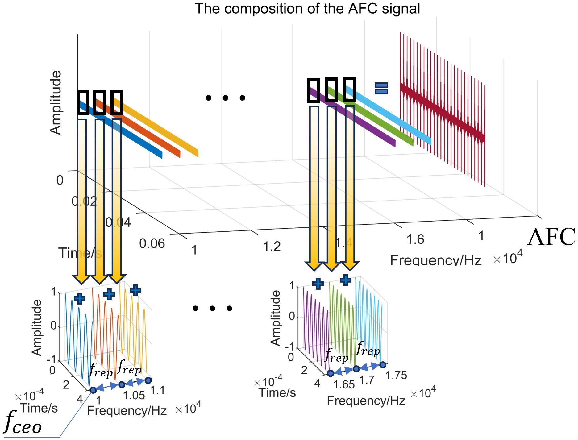
Figure 1 The composition of the AFC signal in the time and frequency domains.

$\begin{array}{ll}s(t)=rect(\frac{t}{T}){\displaystyle {\sum }_{n=1}^{m}A{E}_{n}cos(2\pi f_{n}t+{\theta }_n),}& (1)\end{array}$

$\begin{array}{ll}rect(\frac{t}{T})=\{\begin{array}{c}1, 0\le t\le T,\\ 0,t<0 or t>T,\end{array}& (2)\end{array}$

$\begin{array}{ll}{f}_n=f_{ceo}+(n-1)f_{rep},& (3)\end{array}$

where $rect$ is the rectangular pulse function, t is the time, T is the pulse period, n is an integer, $m$ is the number of modes, A is the power amplification factor, $E_n$ is the amplitude of individual mode, $f_n$ is the frequency of individual mode, ${\theta }_n$ is the initial phase, $f_{ceo}$ is the initial frequency, f_rep is the interval frequency.

The strictly evenly distributed frequency intervals and the extremely precise amplitude and phase lead to the stability of the measurement results with $f_{ceo}$ and $f_{rep}$ well referenced to an Rb clock. Thus, through the coherent superposition of each highly stable frequency component, the pulse signal with a narrow pulse width and high peak power in the time domain can be formed. Each pulse contains all harmonic components and the corresponding frequency and phase information can be calculated by Fourier transform. The echo waveforms of AFC can be expressed as Equation 4:

$\begin{array}{ll}r(t)=a·s[(1+\Delta )(t-2R/c)]+w(t),& (4)\end{array}$

where a is the gain coefficient of the echo intensity, $\Delta$ is the Doppler factor, R is the distance between the signal source and the moving target, c is the velocity of sound, and $w(t)$ is white noise (Equation 5).

$\begin{array}{ll}\Delta =\frac{2v}{c-v}\approx \frac{2v}{c} & (5)\end{array}$

where v is the radial velocity of a moving target.

2.2 Time domain characterization of the Doppler factor

Assume that at time $t_0$, the pulse front of the signal hits a fast-moving target with speed ν and reflects it back. After the time interval of $t_d$, i.e. at moment $t_1$, the pulse back edge hits the moving target. During this time, the target moves the distance $v{t}_d$. According to the quantitative relationship in Figures 2A, B, the following equations can be obtained:

Figure 2

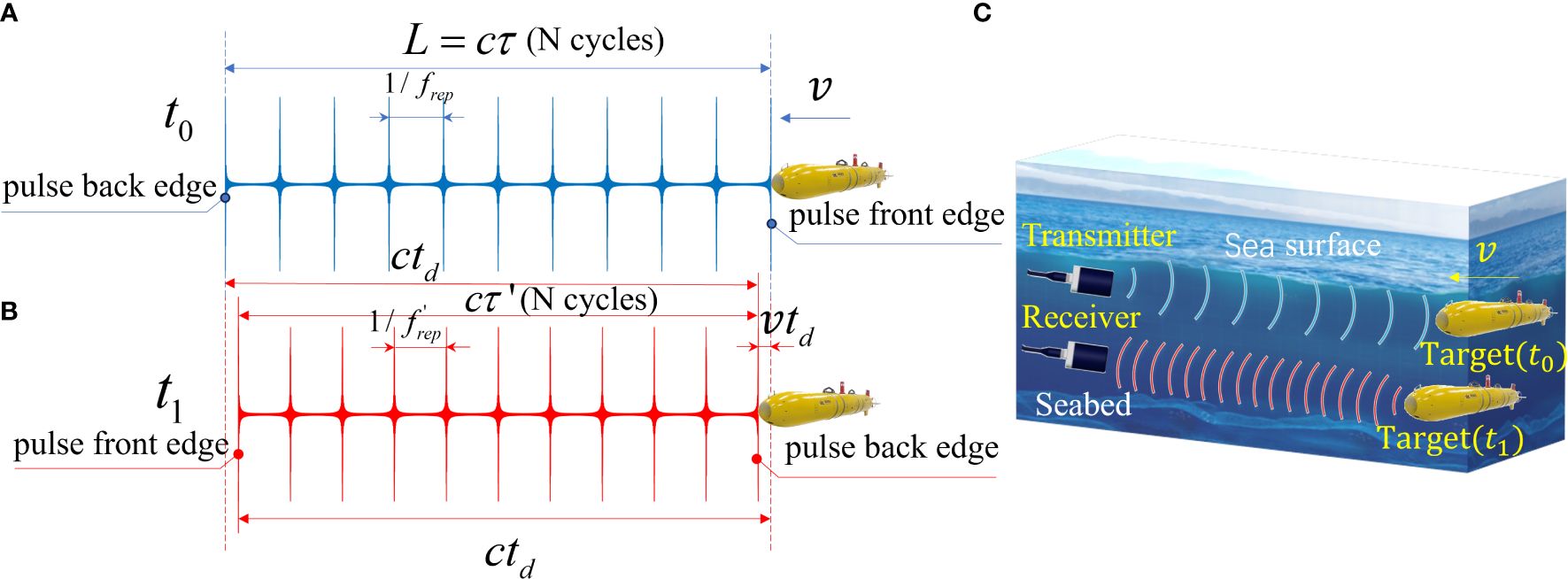
Figure 2 (A) The AFC waveform of the transmitted signal when it first touches the moving target; (B) The AFC waveform of the echo signal when it just leaves the moving target; (C) The time-domain compression phenomenon caused by the Doppler effect.

$\begin{array}{ll}c\tau =c{t}_d+v{t}_d,& (6)\end{array}$

$\begin{array}{ll}c{\tau }^{\prime }=c{t}_d-v{t}_d,& (7)\end{array}$

where c is the velocity of sound, $\tau$ and ${\tau }^{\prime }$are the duration of the emitted and received pulse. From Equation 6 and Equation 7, it can be easily deduced as

$\begin{array}{ll}\frac{\text{τ}}{\text{τ'}}=\frac{c+v}{c-v}.& (8)\end{array}$

Suppose the number of periods of the transmitted signal is $N_T$, obviously with no change in two moments. The $f_{rep}$ and $f_{rep}^{\text{'}}$ can be determined using the following equations:

$\begin{array}{ll}{f}_{rep}=\frac{N_T}{\text{τ}},& (9)\end{array}$

$\begin{array}{ll}{f}_{rep}^{\text{'}}=\frac{N_T}{{\tau }^{\text{'}}}.& (10)\end{array}$

According to Equations 8–10, the equation can be deduced as Equation 11

$\begin{array}{ll}{f}_{rep}^{\text{'}}=\frac{c+v}{c-v}{f}_{rep}=(1+\Delta )f_{rep.}& (11)\end{array}$

The direction of movement of the target is set as positive. As can be seen from Figure 2C, the Doppler effect leads to compression of the AFC signal in the time domain when the target moves toward the transmitter and the receiver. The severity of the Doppler effect can be reflected via the peak intervals of the signal envelope.

3 CUU estimator for the Doppler factor based on AFC waveforms

3.1 Spectrum analysis

Fourier transform is performed on the received signal,

$\begin{array}{ll}X(\omega )=ℱ\left\{r(t)\right\}(\omega )={\displaystyle {\int }_{-\infty }^{\infty }r(t)e^{-j\omega t}dt.} & (12)\end{array}$

According to the linear property and time-shift property of Fourier transform, the Equation 12 can be written as

$\begin{array}{ll}ℱ\left\{r(t)\right\}(\omega )=a·e^{-j\omega \frac{2R}{c}}·ℱ\left\{s[(1+\Delta )t]\right\}(\omega ).& (13)\end{array}$

Due to the time-domain scaling property of the Fourier transform, Equation 13 can be further rewritten as

$\begin{array}{ll}ℱ\left\{r(t)\right\}(\omega )=e^{-j\omega \frac{2R}{c}}·\frac{a}{1+\Delta }·ℱ\left\{s(t)\right\}\left(\frac{\omega }{1+\Delta }\right). & (14)\end{array}$

Set $e^{-j\omega \frac{2R}{c}}·\frac{a}{1+\Delta }$ as β, and make $\frac{\omega }{1+\Delta }$ as ${\omega }^{\prime }$, and the Equation 14 can be written as

$\begin{array}{ll}ℱ\left\{r(t)\right\}(\omega )=\beta ·{\displaystyle {\sum }_{n=1}^mℱ\left\{\cos \left[\frac{2\pi (1+\Delta )f_{n}t}{1+\Delta }\right]\right\}({\omega }^{\prime }). } & (15)\end{array}$

${\omega }^{\prime }$ is changed to $\omega$, and Equation 15 is simplified to

$\begin{array}{ll}ℱ\left\{\text{r}(t)\right\}(\omega )=\beta ·{\displaystyle {\sum }_{\text{n}=1}^{\text{m}}ℱ\left\{\cos (2\pi (1+\Delta )f_{n}t)\right\}(\omega ).} & (16)\end{array}$

Applying the discrete Fourier transform to Equation 16, we can get

$\begin{array}{ll}X(k)=\beta ·{\displaystyle {\sum }_{n=1}^m{\displaystyle {\sum }_{i=0}^{N-1}cos(2\pi (1+\Delta )f_{n}i{T}_s)e^{-j\frac{2\pi ki}{N}}, }}& (17)\end{array}$

where T_s is the sampling interval.

It can be seen from Equation 17, the frequency domain characteristics of the echo signal are the linear superposition of individual phonon signals. Since the phonon modes are Doppler-sensitive single-tone signals, the Doppler factor can be determined by each independent component. This is equivalent to obtaining multiple Doppler factor measurements from just one set of transmitting and receiving pulse signals. The frequency of the received signal can also be expressed as Equation 18:

$\begin{array}{ll}{f}_{rn}=(1+{\Delta }_n)f_n.& (18)\end{array}$

According to the relationship between the repetition frequency and period of the AFC signal, it is also consistent with Equation 11.

The AFC signal consists of multiple signals with separate single-tone components, each affected by the Doppler effect, resulting in the Doppler frequency shift phenomenon. The frequency shift of each phonon mode can be directly calculated by $f_{dn}=f_{rn}-f_n$. $f_{rn}$ can be quickly determined by the FFT of the received signals followed by peak detection, and $f_n$ is the given information of the broadcast signal.

As can be seen from Figure 3A, the frequency shift between the first frequency component of the transmitted waveform and the received waveform is 200 Hz, and the last is 350 Hz. It varies linearly with the frequency of the emitted phonon mode (Figure 3B). The phonon modes of the transmitted signals differ from each other. Still, the variable size of the frequency shift $f_{dn}$ for each frequency component can be determined, corresponding to the same Doppler factor. This means the Doppler factor can be calculated multiple times with just one measurement, leading to a more accurate estimate.

Figure 3

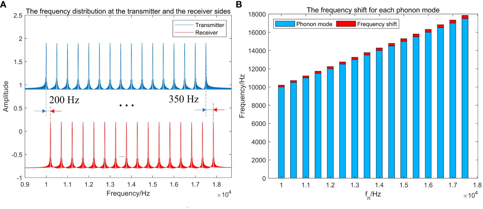
Figure 3 (A) The frequency distribution at both the transmitter and the receiver sides; (B) The frequency shift for each phonon mode.

3.2 System modeling

Different frequency components with the same frequency resolution lead to different deviations for different phonons (Figure 4A). The variance of ${\Delta }_n$ can be deduced as: $D({\Delta }_n)=1/(12f_n^2)$, assuming that the frequency resolution is 1 Hz and the $f_{dn}$ is evenly distributed in the range from -0.5 Hz to 0.5 Hz. To obtain a more precise estimate, we calculate the weight of each measurement by taking the inverse of the variance of ${\Delta }_n$. The sum of these inverses is then utilized to standardize the weight of each measurement. Further derivation of the Doppler factor is as Equation 19

Figure 4

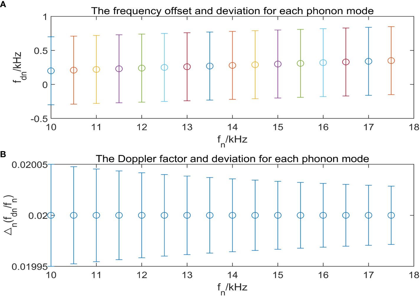
Figure 4 (A) The frequency offset and deviation for each phonon mode; (B) The Doppler factor and deviation with respect to the frequency of phonon mode.

$\begin{array}{ll}\Delta ={\displaystyle {\sum }_{n=1}^m\frac{f_n^2}{{{\displaystyle \sum }}_{n=1}^m{f}_n^2}{\Delta }_{n.}}& (19)\end{array}$

To further clarify the principle of the AFC-based Doppler estimation method, an AFC signal with an initial frequency of 100 kHz, an interval frequency of 500 Hz, a cutoff frequency of 200 kHz, and an initial phase of 0 rad for all phonon modes is constructed. The Doppler factor is set to 0.02 with a frequency resolution of 1 Hz, and the duration is set at 50 ms. The received signal in the time domain is transformed by FFT. The uncertainty of each individual phonon mode can be induced by the frequency resolution, and all Doppler shifts correspond to the same Doppler factor. This distortion can be eliminated by multiple unequal precision measurements (Figure 4B), a mode similar to the principle of the CUU estimation method.

As shown in Figure 5, as δ ranges from 0.05 to 0.45, which is the ratio of offset frequency to frequency resolution, the bias of single-tone signal after FFT does not exceed 3.2×10^-5. While the AFC-based method keeps a bias of less than 1.1×10^-5. Traditional Doppler factor estimation using single-tone waveforms is limited by the number of samples of the Fourier transform N, which inevitably leads to the spectral leakage. However, the use of AFC waveforms can enable the acquisition of multiple different Doppler factor values across different phonon modes, which is equivalent to carrying out numerous measurements of the identical Doppler factor simultaneously. In this way, the utilization of the spectrum has been significantly improved. It can be further reduced by increasing the number of phonon modes, and there is almost no additional computational effort.

Figure 5

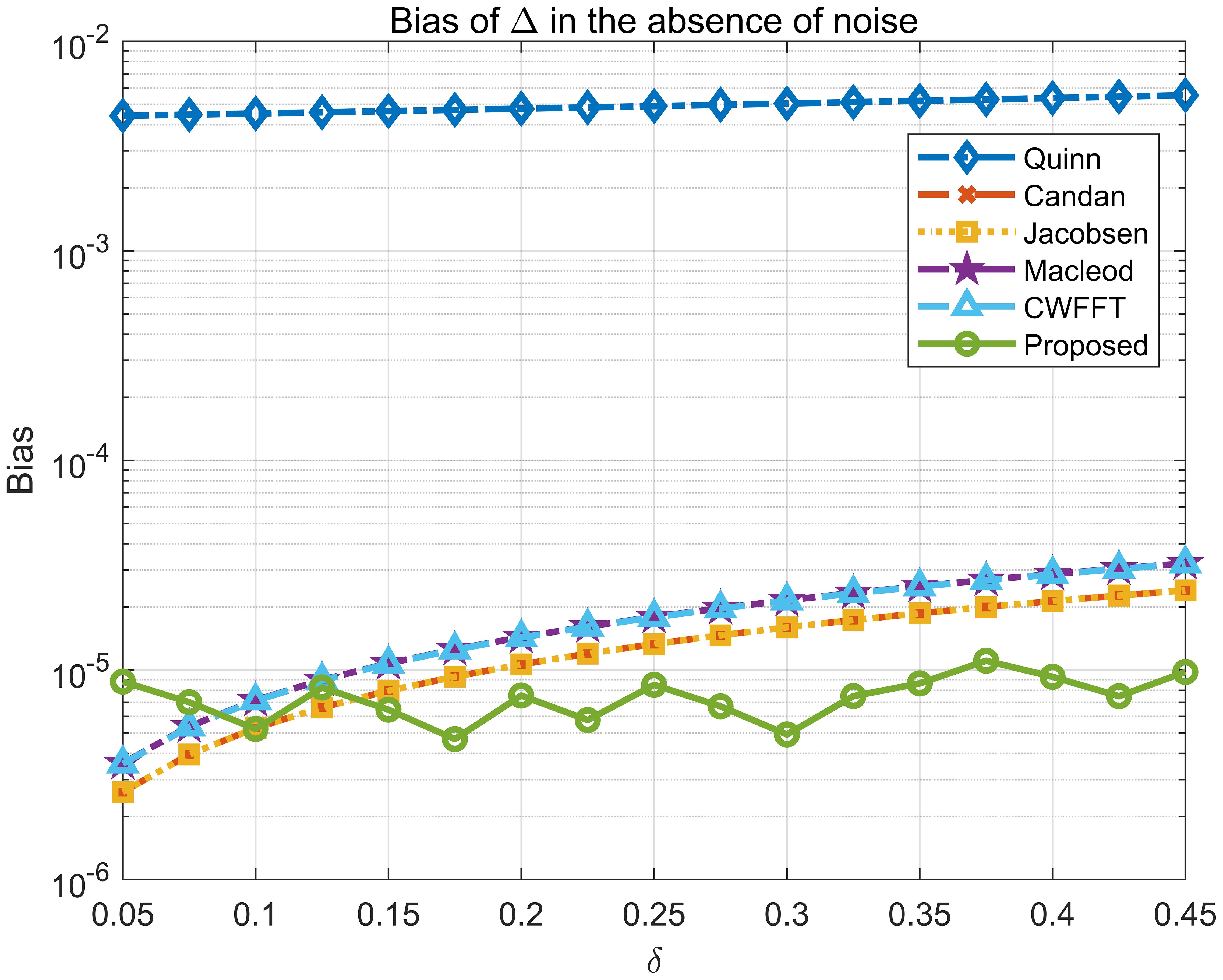
Figure 5 Bias of different estimators in the absence of noise.

4 Numerical section

4.1 Experimental parameters

To demonstrate the effectiveness of the proposed method, two sets of Monte Carlo experiments were conducted using the methods listed in Table 1, which were repeated 1000 times. In the experiments, the duration of the single-tone signals and the AFC signal were both set at 50 ms. The AFC was set with a starting frequency of 10 kHz, a cutoff frequency of 17.5 kHz, and an interval frequency of 0.5 kHz, the frequency of the single-tone signal was set to 14 kHz, the sampling rate and the sampling number were set to 96 kHz. The conditions for two series of tests were set as follows:

Table 1

Table 1 Estimation expressions of different methods.

1) Keep δ of the single-tone signals unchanged at 0.45, convert it to an equivalent Doppler factor, and gradually increase the input signal-to-noise ratio (SNR) from -2 dB to 10 dB. Observe the bias and the root mean square error (RMSE);

2) The number of sampling points was reduced to half of the previous, and other parameters remained the same as in experiment 1. Observe the RMSE with SNR.

The Cramer-Rao bound (CRB) can be used to indicate the best-estimated performance, although it is not typically applicable for biased estimators. It can be expressed by Equation 20

$\begin{array}{ll}var(\widehat{f})\ge CRB=\frac{3f_s^2}{2{\pi }^{2}N(N^2-1)SNR}, & (20)\end{array}$

where f_s is the sampling frequency. The variance of the Doppler factor can be obtained through the variance transfer formula.

4.2 Numerical results

As shown in Figure 6, the deviation of the true Doppler factor by the CUU method based on AFC does not exceed 1.1×10^-5 when δ is 0.45. In contrast, alternative frequency estimation methods have a minimal bias of 1.5×10^-5 and a maximal bias of 5.3×10^-5. It is noteworthy that the CUU method has a bias with a maximum value that is smaller than the minimum value observed in other frequency estimation methods.

Figure 6

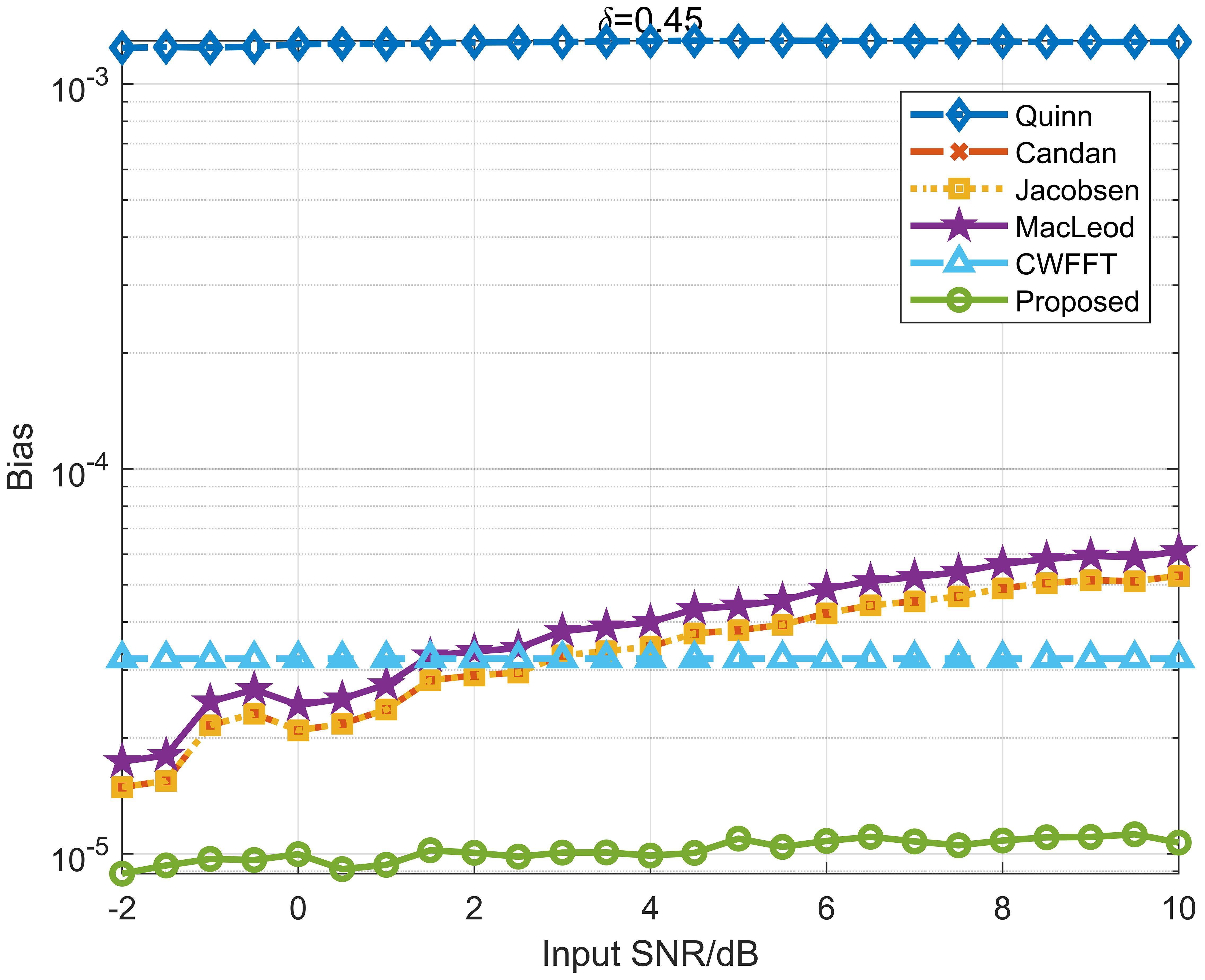
Figure 6 Variation of bias with respect to SNR for δ = 0.45 with a frequency resolution of 2 Hz.

Figure 7 demonstrates that at a frequency resolution of 1 Hz, the RMSE of the proposed method is no greater than 1.5×10^-5, significantly lower than 2.9×10^-5 observed with other frequency estimation methods. At a frequency resolution of 2 Hz, the RMSE for the proposed method is lower than 1.8×10^-5, better than 6.0×10-5 for other methods, as shown in Figure 8. In both scenarios, the RMSE of the AFC-based method is closer to the CR bound, showing the high accuracy and robustness of the CUU method based on AFC.

Figure 7

Figure 7 Variation of RMSE with respect to SNR for δ = 0.45 with a frequency resolution of 1 Hz.

Figure 8

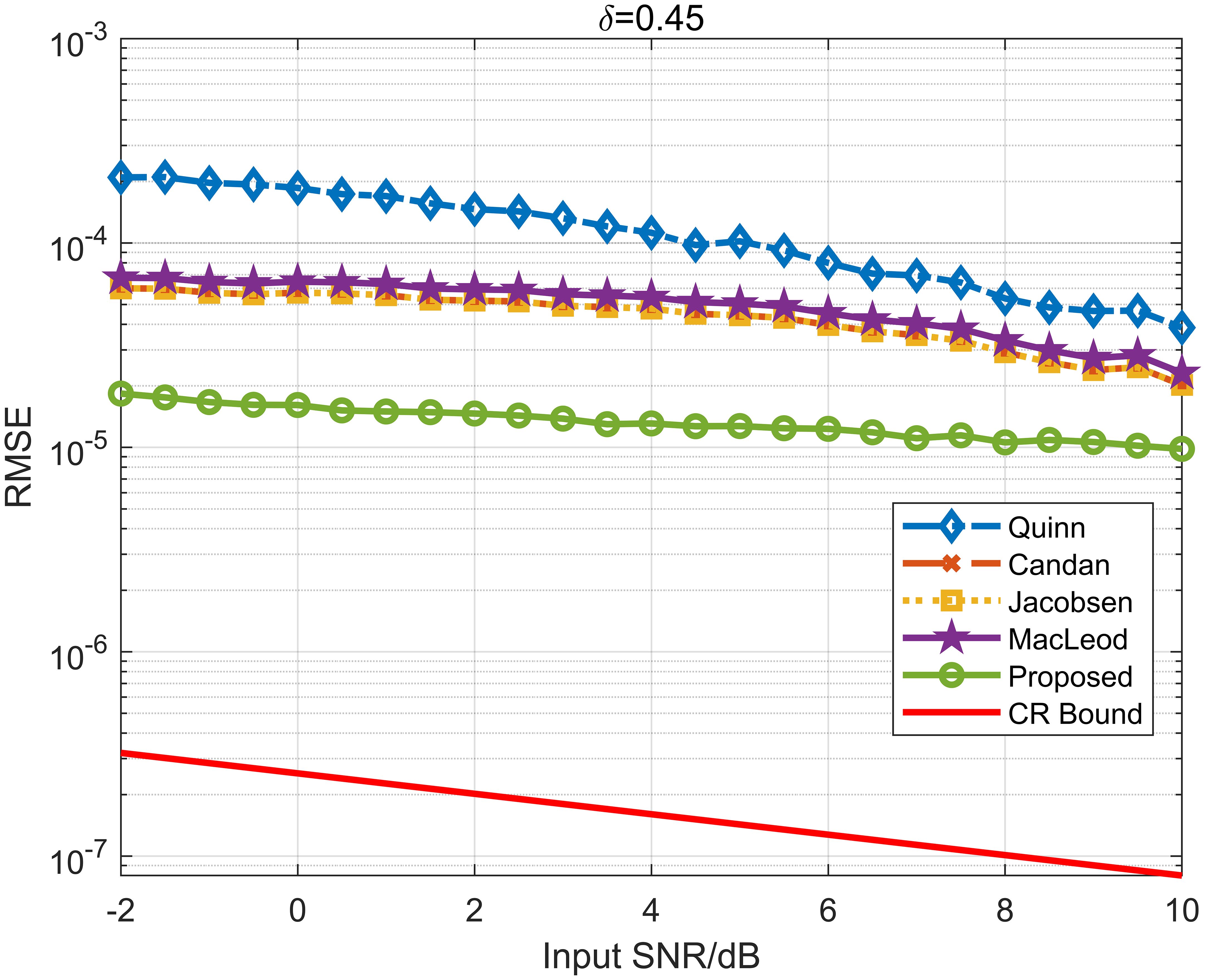
Figure 8 Variation of RMSE with respect to SNR for δ = 0.45 with a frequency resolution of 2 Hz.

4.3 Experimental results

In order to provide further validation for the effectiveness of the proposed method, Watermark, a widely accessible benchmark for physical-layer techniques in underwater acoustic communications, was employed. This benchmark is based on empirical measurements of the time-varying impulse response collected at sea (van Walree et al., 2017).

The Norway-Oslofjord (NOF1) channel with the large available bandwidth was selected to validate the practical efficacy of underwater communication. In the single-input single-output (SISO) scenario, the time-varying impulse response (TVIR) of the transmitted signal affected by the Doppler effect is obtained, and the signal packet is retrieved through serial acquisition processes. The signal has been established with a SNR of 20 dB, a pulse length of 50 ms, a frequency resolution of 1Hz, and other parameters consistent with the first Monte Carlo experiment in Section 4.1. Figure 9A demonstrates that due to the frequency-selective fading of underwater acoustic channels, the magnitude of each frequency component varies, while the AFC signal spectrum remains uniformly spaced. By calculating the Doppler shift based on frequency rather than phase, the impact of multipath effects is limited. Contrary to conventional methods that primarily focus on spectral peaks and their adjacent lines while disregarding the remaining spectrum, our proposed approach considers signals from different frequencies under the influence of the same Doppler effect, leading to distinct spectral peaks at various positions on the spectrum. Unlike the singular spectral peak observed in CW signal circumstance (Figure 9B), each spectral peak of the AFC signal effectively reflects the potency of the Doppler effect. The cumulative effect of multiple measurements leads to the estimation of the Doppler factor aligning closely with the true value, thereby enhancing the accuracy of estimation and resulting in improved estimation precision (Figure 9C). The difference of the CUU method utilizing the AFC signal is below 3.4×10^-6, notably lower than that of the 3.2×10^-5 induced by spectral leakage.

Figure 9

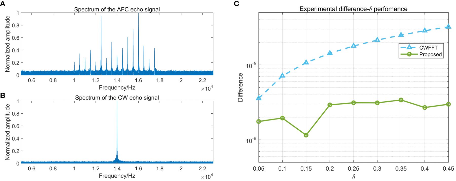
Figure 9 (A) The spectrum of the AFC echo signal; (B) The spectrum of the CW echo signal; (C) The experimental difference-δ performance.

4.4 Computational burden

Table 2 shows the calculation scales of the methods. It can be seen that the computational cost of the proposed algorithm is lower than that of other frequency estimation methods for single-tone signals. The proposed method does not require additional complex multiplication and complex addition, and it achieves a better Doppler estimation performance. Essentially, this is because the CUU method makes full use of spectrum information.

Table 2

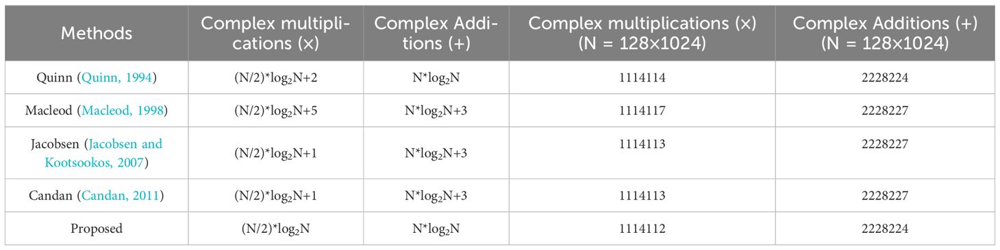
Table 2 The computational requirements of different methods.

5 Conclusion

In this paper, we proposed a novel acoustic broadband signal, AFC, to estimate the Doppler factor of underwater acoustic applications. The quantitative relationship between the AFC and the Doppler factor in the time and frequency domains was derived theoretically. At the expense of bandwidth, the phonon frequency shifts of multiple frequency components can be determined by one measurement, allowing the Doppler factor to be calculated multiple times simultaneously, resulting in a precise Doppler estimate. The proposed method maintains a low computational cost and improved spectral leakage performance by means of CUU. Besides, the uncertainty can be calculated from a single measurement, not available with other methods.

The AFC-based method keeps a bias of less than 1.1×10^-5, while the bias of single-tone signal after performing FFT does not exceed 3.2×10^-5 in the absence of noise. In the presence of additive white Gaussian noise, the bias of the AFC-based CUU method is less than 1.1×10^-5, significantly lower than the observed bias of 5.3×10^-5 with other estimation methods at a frequency resolution of 1 Hz. The RMSE of the proposed method is no greater than 1.5×10^-5, significantly lower than 2.9×10^-5 observed with other frequency estimation methods. At a frequency resolution of 2 Hz, the RMSE for the proposed method is 1.8×10^-5, compared to 6.0×10^-5 for other methods. In the SISO scenario of Watermark, The difference of the CUU method utilizing the AFC signal is below 3.4×10^-6, notably lower than that of the 3.2×10^-5 induced by spectral leakage in FFT. Both numerical simulations and experimental results demonstrate that the CUU method based on AFC outperforms traditional frequency estimation methods for single-tone signals in terms of accuracy and computational efficiency. This introduces a new platform for acoustic applications and enhances the accuracy of Doppler estimation.

Data availability statement

The raw data supporting the conclusions of this article will be made available by the authors, without undue reservation.

Author contributions

JL: Visualization, Writing – original draft, Writing – review & editing. ZQ: Formal analysis, Supervision, Writing – original draft. DH: Investigation, Visualization, Writing – original draft. JZ: Conceptualization, Methodology, Writing – original draft.

Funding

The author(s) declare financial support was received for the research, authorship, and/or publication of this article. This work was supported by Open Fund Projects of Key Laboratory of Marine Environmental Survey Technology and Application (MESTA-2023-B006), Basic Science Centre Project of the National Natural Science Funding Council (62388101) and the Natural Science Foundation of Tianjin (22JCQNJC00270).

Acknowledgments

Special thanks to the funding that provided support for this research.

Conflict of interest

The authors declare that the research was conducted in the absence of any commercial or financial relationships that could be construed as a potential conflict of interest.

Publisher’s note

All claims expressed in this article are solely those of the authors and do not necessarily represent those of their affiliated organizations, or those of the publisher, the editors and the reviewers. Any product that may be evaluated in this article, or claim that may be made by its manufacturer, is not guaranteed or endorsed by the publisher.

References

Aboutanios E., Mulgrew B. (2005). Iterative frequency estimation by interpolation on Fourier coefficients. IEEE Trans. Signal Processing 53, 1237–1242. doi: 10.1109/TSP.2005.843719

CrossRef Full Text | Google Scholar

Ahmad A. M., Kassem J., Barbeau M., Kranakis E., Porretta E., Garcia-Alfaro J. (2018). Doppler effect in the acoustic ultra low frequency band for wireless underwater networks. Mobile Networks Applications 23, 1282–1292. doi: 10.1007/s11036-018-1036-9

CrossRef Full Text | Google Scholar

Braje D. A., Kirchner M. S., Osterman S., Fortier T., Diddams S. A. (2008). Astronomical spectrograph calibration with broad-spectrum frequency combs. Eur. Phys. J. D. 48, 57–66. doi: 10.1140/epjd/e2008-00099-9

CrossRef Full Text | Google Scholar

Candan Ç. (2011). A method for fine resolution frequency estimation from three DFT samples. IEEE Signal Process. Letters 18, 351–354. doi: 10.1109/LSP.2011.2136378

CrossRef Full Text | Google Scholar

Chan Y. T., Jardine F. L. (1990). Target localization and tracking from Doppler-shift measurements. IEEE J. Oceanic Engineering 15, 251–257. doi: 10.1109/48.107154

CrossRef Full Text | Google Scholar

Chen Y., Yin J., Zou L., Yang D., Cao Y. (2015). Null subcarriers based Doppler scale estimation with polynomial interpolation for multicarrier communication over ultrawideband underwater acoustic channels. J. Syst. Eng. Electronics 26, 1177–1183. doi: 10.1109/JSEE.2015.00128

CrossRef Full Text | Google Scholar

Fang L., Duan D., Yang L. (2012). A new DFT-based frequency estimator for single-tone complex sinusoidal signals. In MILCOM 2012-2012 IEEE Military Commun. Conference 8, 1–6. doi: 10.1109/MILCOM.2012.6415812

CrossRef Full Text | Google Scholar

Gong Z. J., Li C., Jiang F. (2020). Analysis of the underwater multi-path reflections on Doppler shift estimation. IEEE Wireless Commun. Letters 9, 1758–1762. doi: 10.1109/LWC.5962382

CrossRef Full Text | Google Scholar

Greene A. D., Hendricks P. J. (2015). Using an ADCP to estimate turbulent kinetic energy dissipation rate in sheltered coastal waters. J. Atmospheric Oceanic Technol 32, 318–333. doi: 10.1175/JTECH-D-13-00207.1

CrossRef Full Text | Google Scholar

Hall J. L. (2006). Nobel lecture: defining and measuring optical frequencies. Rev. Modern Physics 78, 1279–1295. doi: 10.1103/RevModPhys.78.1279

CrossRef Full Text | Google Scholar

Hansch T. W. (2006). Nobel lecture: passion for precision. Rev. Modern Physics 78, 1297–1309. doi: 10.1103/RevModPhys.78.1297

CrossRef Full Text | Google Scholar

Jacobsen E., Kootsookos P. (2007). Fast, accurate frequency estimators [DSP Tips & Tricks]. IEEE Signal Process. Magazine 24, 123–125. doi: 10.1109/MSP.2007.361611

CrossRef Full Text | Google Scholar

Jones D. J., Diddams S. A., Ranka J. K., Stentz A., Windeler R. S., Hall J. L., et al. (2000). Carrier-envelope phase control of femtosecond mode-locked lasers and direct optical frequency synthesis. Science 288, 635–639. doi: 10.1126/science.288.5466.635

PubMed Abstract | CrossRef Full Text | Google Scholar

Kay S. (1989). A fast and accurate single frequency estimator. IEEE Trans. Acoustics Speech Signal Processing 37, 1987–1990. doi: 10.1109/29.45547

CrossRef Full Text | Google Scholar

Li Y., Chen K. (2008). Eliminating the picket fence effect of the fast Fourier transform. Comput. Phys. Commun. 178, 486–491. doi: 10.1016/j.cpc.2007.11.005

CrossRef Full Text | Google Scholar

Macleod M. D. (1998). Fast nearly ML estimation of parameters of real or complex single tones or resolved multiple tones. IEEE Trans. on Signal Process 46, 141–148. doi: 10.1109/78.651200

CrossRef Full Text | Google Scholar

Mikhail Z., David S., Paola G.-P., Carolina G. (2014). Efficient CO₂ fixation by surface Prochlorococcus in the Atlantic Ocean. ISME J. 83, 2280–2289. doi: 10.1038/ismej.2014.56

CrossRef Full Text | Google Scholar

Quinn B. G. (1994). Estimating frequency by interpolation using Fourier coefficients. IEEE Trans. Signal Processing 42, 1264–1268. doi: 10.1109/78.295186

CrossRef Full Text | Google Scholar

Rife D., Boorstyn R. (1974). Single-tone parameter estimation from discrete-time observations. IEEE Trans. Inf. Theory 20, 591–598. doi: 10.1109/TIT.1974.1055282

CrossRef Full Text | Google Scholar

Sen S., Nehorai A. (2010). Adaptive design of OFDM radar signal with improved wideband ambiguity function. IEEE Trans. Signal Processing 58, 928–933. doi: 10.1109/TSP.2009.2032456

CrossRef Full Text | Google Scholar

Sharif B. S., Neasham J., Hinton O. R., Adams A. E. (2000). A computationally efficient Doppler compensation system for underwater acoustic communications. IEEE J. Oceanic Engineering 25, 52–61. doi: 10.1109/48.820736

CrossRef Full Text | Google Scholar

Steinmetz T., Wilken T., Araujo-Houck C., Holzwarth R., Haensch T. W., Pasquini L., et al. (2008). Laser frequency combs for astronomical observations. Science 321, 1335–1337. doi: 10.1126/science.1161030

PubMed Abstract | CrossRef Full Text | Google Scholar

van Walree P. A., Socheleau F. X., Otnes R., Jenserud T. (2017). The watermark benchmark for underwater acoustic modulation schemes. IEEE J. oceanic engineering 42, 1007–1018. doi: 10.1109/JOE.2017.2699078

CrossRef Full Text | Google Scholar

Wan L., Jia H., Zhou F., Muzzammil M., Li T., Huang Y. (2020). Fine Doppler scale estimations for an underwater acoustic CP-OFDM system. Signal Processing 170, 107439. doi: 10.1016/j.sigpro.2019.107439

CrossRef Full Text | Google Scholar

Wu H., Qian Z., Zhang H., Xu X., Xue B., Zhai J. (2019). Precise underwater distance measurement by dual acoustic frequency combs. Annalen der Physik 531, 1900283. doi: 10.1002/andp.201900283

CrossRef Full Text | Google Scholar

Yang P. X. (2023). An imaging algorithm for high-resolution imaging sonar system. Multimedia Tools Applications 83, 1–16. doi: 10.1007/s11042-023-16757-0

CrossRef Full Text | Google Scholar

Yang Y., Fang S. (2021). Dynamic optimization method for broadband ADCP waveform with environment constraints. Sensors 21, 3768. doi: 10.3390/s21113768

PubMed Abstract | CrossRef Full Text | Google Scholar

Zhang X. B. (2023). An efficient method for the simulation of multireceiver SAS raw signal. Multimedia Tools Applications 83, 1–17. doi: 10.1007/s11042-023-16992-5

CrossRef Full Text | Google Scholar

Zhang X. B., Wu H., Sun H., Ying W. (2021). Multireceiver SAS imagery based on monostatic conversion. IEEE J. Selected Topics Appl. Earth Observations Remote Sensing 14, 10835–10853. doi: 10.1109/JSTARS.2021.3121405

CrossRef Full Text | Google Scholar

Zhang X. B., Yang P., Wang Y., Shen W., Yang J., Wang J., et al. (2024). A novel multireceiver SAS RD processor. IEEE Trans. Geosci. Remote Sensing. 62, 1–11. doi: 10.1109/TGRS.2024.3362886

CrossRef Full Text | Google Scholar