A physics-informed machine learning approach for predicting acoustic convergence zone features from limited mesoscale eddy data

Mesoscale eddies are prevalent mesoscale phenomena in the oceans that alter the thermohaline structure of the ocean, significantly impacting acoustic propagation patterns. Accurately predicting acoustic convergence zone features has become an urgent task, especially when data are limited in deep-sea mesoscale eddy environments. This study utilizes physics-informed machine learning to identify and predict the acoustic convergence zone features of mesoscale eddies under limited data conditions. Initially, a method based on convex hull ratio was utilized to identify mesoscale eddies from the JCOPE2M reanalysis dataset and AVISO data in the Kuroshio‐Oyashio Extension. Subsequently, by integrating physical models and ray acoustics, relevant features of mesoscale eddies and convergence zones are extracted. Then, K-fold cross-validation and sparrow search algorithms are employed to select the optimal machine learning algorithm, ensuring high model accuracy. The resulting model requires only a thermohaline profile near the eddy center and sea surface height to predict convergence zone features within the mesoscale eddy environment, achieving a MAE of approximately 1.00 km and an accuracy (within 3 km) exceeding 95%. Additionally, leveraging physics-informed machine learning methods contributes to a maximum reduction of 0.82 km in MAE and an improvement in accuracy by 2.80% to 11.92% compared to models without physical information input. Finally, the model’s validity and reliability in the actual ocean environment are verified by cross-validating it with data from various sea regions" in bright yellow and Argo profiling float data. The findings provide novel insights into acoustic propagation in mesoscale eddy environments and subsequent ocean acoustic research.

1 Introduction

Mesoscale eddies are a common type of phenomenon in the global ocean. They can last from a few days to several hundreds of days and can range in size from tens to hundreds of kilometers (Chelton et al., 2011). These eddies have a significant impact on the distribution of various oceanic properties such as temperature, salinity, chlorophyll, dissolved oxygen, and nutrients (Barone et al., 2021). They also induce upwelling and downwelling within their regions, leading to the horizontal and vertical movement of oceanic materials (Zhao et al., 2021). Additionally, the distinct mass properties of mesoscale eddies cause the cold and warm water they carry to affect the speed of sound, thus influencing the propagation of sound waves through seawater (Etter, 2013). Therefore, studying the acoustic propagation characteristics of mesoscale eddies in the ocean is crucial for underwater sonar detection, planning acoustic anti-submarine warfare missions, submarine stealth, and early warning detection.

The Kuroshio Extension (KE) is the eastward branch of the powerful western boundary current known as the Kuroshio Current at 35°N, and spanning eastward to approximately 160°E. It also mixes with Oyashio water from high-latitude sea areas and shares the same characteristics as the Kuroshio: high temperature, high salinity, high color of water, high clarity, and fast current speed. Additionally, it is a key area for mid-latitude sea-air interaction and one of the sea areas with the highest eddy kinetic energy and the most active mesoscale eddy features (Scharffenberg and Stammer, 2010). Depending on the generation mechanism, the mesoscale eddies in the KE region are partially shed from the KE. These can be considered closed water masses, with the nature of water masses playing a crucial role in the region for heat, eddies, and material transport (Chelton et al., 2011). Using satellite altimeter data and Argo data, previous studies have detailed the basic characteristics of the eddies in the KE region. Additionally, more anticyclonic eddies are present on the north side of the KE, moving at a speed of approximately 1–2 cm/s, with longer life cycles. Meanwhile, more cyclonic eddies are detected on the south side of the KE and near the flow axis. These eddies move at a speed of approximately 1–5 cm/s and possess stronger intensity (Itoh and Yasuda, 2010). Furthermore, according to years of satellite altimeter data, the eddy kinetic energy of mesoscale eddies in the region is characterized by strength in summer and weak in winter (Scharffenberg and Stammer, 2010), and its inter-decadal variations are positively correlated with the Pacific Decadal Oscillation (PDO) index. When the PDO is positive, the eddy kinetic energy in the region is strong, and vice versa (Taguchi et al., 2010).

Numerous researchers have devoted to understanding the effects of mesoscale eddy environments on underwater acoustic propagation. They have explored the relationship between eddies and acoustic propagation through observations and experiments. Akulichev, Bugaeva (Akulichev et al., 2012) reported the results of an acoustic survey in the KE region of the NW Pacific Ocean. They found that a mesoscale eddy significantly affected the horizontal propagation of acoustic signals through a towed source at a depth of 100 m. Liu, Piao (Liu et al., 2021) detected and tracked a mesoscale eddy in the western North Pacific Ocean, studying the eddy strength, oceanographic, and acoustic characteristics. Their study revealed that the position of the convergence zone (CZ) shifted away from the source or near the source when cyclonic and anticyclonic eddies propagated sound. Additionally, the coupling coefficients of different-order normal modes also underwent significant changes during this process. Some studies utilized physical modeling and numerical simulation methods to examine the sound speed field distribution and propagation characteristics in mesoscale eddy environments. Xiao, Li (Xiao et al., 2018) statistically analyzed the underwater acoustic sound propagation characteristics in deep-sea mesoscale eddy environments using a parabolic model. They evaluated the effect of several factors such as the relative positions of sound sources and eddies on underwater acoustic sound propagation. Mahpeykar, LARKI (Mahpeykar et al., 2022) used ray acoustics to analyze the effect of mesoscale eddies on underwater acoustic propagation in the Persian Gulf. They observed that the presence of cyclonic eddies increased the transmission loss (TL), which further increased with the depth of the sound source passing through the mesoscale eddies. Xiao, Lei (Xiao et al., 2021) developed a theoretical model of acoustic propagation under the influence of oceanic mesoscale eddies using finite element analysis. They discovered that the distance from sound source to CZ decreases when acoustic energy emitted by the sound source passes through an anticyclonic eddy. Similarly, Liu, Piao (Liu et al., 2021) used a ray model, while Chen, Hong (Chen et al., 2019) reached the same conclusion after simulating in-situ oceanographic data using the University of Miami Parabolic Equation model.

With the rapid development of computer technology, machine learning has gained remarkable results in multiple fields such as underwater acoustics and oceanography (Doan et al., 2020; Yang et al., 2020; Jiang and Zhu, 2022; Sadaiappan et al., 2022). It has been fully applied in research related to mesoscale eddies. Wang, Wang (Wang et al., 2020) constructed a predictive model for mesoscale eddy features and trajectories using the Long Short Term Memory network alongside the Extremely Randomized Trees. The root mean square error between the predicted and actual longitude (latitude) of the trajectory ranges from 28.8 km–47.2 km (23.8 km–37.2 km). Duo, Wang (Duo et al., 2019) developed a mesoscale eddy automatic identification and localization network based on the object detection network, thereby addressing the challenges posed by small samples and complex regions of mesoscale eddies. They also designed and optimized the object detection model using the deep residual network and feature pyramid network as the main structure, achieving a significantly improved recognition performance. However, challenges persist in the research and application of machine learning in mesoscale eddy environments. On one hand, machine learning relies on establishing input and output datasets for the model, posing a gap in how to introduce suitable features to enhance the model’s generalization ability and physical credibility. On the other hand, the CZ waveguide stands as a crucial underwater acoustic propagation mode in the deep ocean environment, significantly impacted by mesoscale eddies (Chen et al., 2022). The current predicament lies in the difficulty faced by vessels traversing far-sea routes within mesoscale eddies to access real-time comprehensive oceanic information pertaining to these phenomena. Consequently, there is a pressing need to investigate the feasibility of utilizing limited mesoscale eddy data for ensuring underwater acoustic propagation assurance. Presently, the prediction and assurance of underwater acoustic environments within mesoscale eddies heavily hinge on the availability of complete oceanic parameters for accurate simulation and modeling. However, in instances where mesoscale eddy data are scarce or absent, maintaining optimal underwater acoustic performance poses significant challenges. Machine learning can potentially predict CZ features by fitting some mesoscale eddy features. Nevertheless, the extent of this predictive capability requires further exploration and verification.

To address the aforementioned concerns, this study proposes a predictive model of CZ features in mesoscale eddy environments based on physics-informed machine learning (PIML), exemplified in the Kuroshio-Oyashio Extension region. This model integrates prior knowledge of physics with data-driven machine learning models, offering an effective approach to mitigate the lack of training data, enhance the model’s generalization capability, and ensure the credibility of the results (Meng et al., 2022). This study expands the acoustic features of mesoscale eddies by incorporating relevant prior physical knowledge and utilizing methods such as Snell’s law and Gaussian eddy modeling. This approach improves data efficiency and enhances the rationality of the model, further exploiting the potential for enhancing traditional analysis and modeling.

2 Data and methods

This study initially proposes a mesoscale eddy identification method based on the convex hull ratio. This method is employed to identify and screen the mesoscale eddies within the KE region using the high-resolution reanalysis data Japan Coastal Ocean Predictability Experiment 2 Modified (JCOPE2M) and the mesoscale eddy datasets provided by Archiving, Validation and Interpretation of Satellite Oceanographic (AVISO). Physical modeling and ray acoustics are used to extract features of mesoscale eddies and CZ for constructing the prediction dataset. Subsequently, 20 machine learning algorithms are screened using K-fold cross-validation and the Sparrow Search Algorithm (SSA), and the most accurate algorithm is selected through various evaluation indexes to construct the predictive model of CZ features in the mesoscale eddy environment. Finally, the predictive model is validated by integrating the Oyashio Extension (OE) region’s mesoscale eddies and Argo data, as depicted in Figure 1. Notably, when predicting the CZ features under a mesoscale eddy environment, considering practical application scenarios and the model’s extension value, the input data comprise a thermohaline contour near the center of the eddy and the sea surface height data. The study focuses on the CZ features of a sound source located within mesoscale eddy environments.

Figure 1

Figure 1 Research approach and workflow for CZ prediction model establishment. (The slice map of mesoscale eddy is derived from JCOPE2M data from January 1, 2020, and the three-dimensional structure of sound propagation is based on simulation results from Bellhop applied to this data.).

2.1 Data

2.1.1 Reanalysis data

The high-resolution reanalysis dataset, JCOPE2M, covers the western North Pacific Ocean with a temporal resolution of 1 day and a horizontal resolution of 1/12°, divided vertically into 46 σ-layers (Miyazawa et al., 2017; Miyazawa et al., 2019). High-resolution satellite sea surface temperature data, sea surface height anomaly data, and in-situ data were assimilated into the model by using the multi-scale three-dimensional variational method. It is more widely used in studying mesoscale phenomena and flow fields (Chang et al., 2015; Chang et al., 2018; Liu et al., 2019). In this study, we utilized temperature and salinity data from the dataset covering the geographical coordinates of 137°E-165°E and 31°N-43°N, collected between 2012 and 2021. These data were employed to compute the sound speed field environment using an empirical formula for sound speed. Additionally, sea surface height data in this dataset are utilized to assist in identifying mesoscale eddies, providing significant reference value in localizing these eddies, despite the discrepancy between the sea surface height data and the actual measurements.

2.1.2 Mesoscale eddy data

The eddy dataset is based on eddy data detected by Chelton, Schlax (Chelton et al., 2011), using multi-year AVISO satellite altimetry data with a temporal resolution of 1 day and a spatial resolution of 0.25° × 0.25°. They employed a program to automatically select a sea surface height threshold and then detected closed sea surface height profiles defined as mesoscale eddies within the threshold range. In order to ensure the accuracy of identification, mesoscale eddies in the JCOPE2M dataset were identified based on convex hull ratio. Following this process, the mesoscale eddy data were compared and filtered against the mesoscale eddy data obtained from the JCOPE2M sea surface height dataset. Only the mesoscale eddy data whose eddy centers in the reanalysis data deviated less than 1° from the eddy centers in the dataset provided by Chelton, Schlax (Chelton et al., 2011) were retained. After screening, data from 2012 to 2021, totaling 29,245 mesoscale eddies (13,849 cyclonic eddies and 15,396 anticyclonic eddies) were selected for this study.

2.1.3 Argo data

The Array for Real-time Geostrophic Oceanography (Argo) is a real-time observational network comprising multiple floats placed across the ocean, aimed at acquiring quasi-real-time, large-scale, high-resolution observations of the global ocean subsurface (Roemmich et al., 2009). As Argo floats descend and ascend, they gather data on the temperature and salinity of the water. Some floats also measure additional properties related to the ocean’s biology and chemistry. This study primarily utilizes temperature and salinity data provided by 10,120 Argo floats between 2012 and 2021, focusing on measurements within mesoscale eddies. There were 5,506 floats positioned inside anticyclonic eddies and 4,614 inside cyclonic eddies.

2.1.4 Terrain data

The seafloor topographic model ETOPO1, provided by the National Centers for Environmental Information (NCEI), is utilized for underwater acoustic modeling and simulation within the study area. With a spatial resolution of 1’, this model integrates a vast array of pertinent modeled and in-situ regional data, encompassing land topography and ocean depth data from across the world (Amante and Eakins, 2009).

2.2 Methodology

2.2.1 Mesoscale eddy identification methods

In this study, the Sea Surface Height (SSH) closed contour method is proposed for mesoscale eddy identification under the constraint of convex hull ratio. Firstly, it calculates all the contours in the study area within the contour interval of -150 cm–150 cm in step size of 1 cm, filters the closed contours, and computes the convex hull ratio of r_c for each contour separately. To ensure the alignment between the identification results and the features of mesoscale eddies and prevent the inclusion of elongated fronts or eddy filaments, only the closed contours of r_c<1.2 are retained in this study. The contours are grouped based on the mesoscale eddies they correspond to, and the outermost closed contour of each group containing the center of the eddy serves as the outer edge of the eddy. The advantage of this method lies in its simplicity, clear physical features, absence of required man-made parameters, and its capability to identify and track mesoscale eddies solely using the SSH observed by satellite altimeter. The formula is as follows, where S represents the area of the closed contour and S_convex represents the area of the convex envelope of the closed contour (Equation 1).

$\begin{array}{ll}{r}_c=S_{convex}/S& (1)\end{array}$

Due to the large study area of this study, obvious differences are present in the properties of the water masses of the KE and the OE, alongside the complex interactions of the eddies within them (Yao et al., 2023). Therefore, the study area is divided into 2 regions as illustrated in Figure 2: the KE 31°-38°N, 137°-165°E (Region I) and the OE 38°-43°N, 142°-165°E (Region II).

Figure 2

Figure 2 (A) Identification of mesoscale eddies in the Kuroshio‐Oyashio Extension region on January 1, 2020. The red closed contour represents the outer boundary of the identified mesoscale eddies, and the green circles indicate the positions of the eddy centers. (B) Distribution map of the positions of the mesoscale eddy center obtained by comparing the identification results of the closed contours based on JCOPE2M SSH data with the selected AVISO data.

2.2.2 Calculation methods for underwater acoustic propagation

Prior to underwater acoustic simulation, the JCOPE reanalysis temperature and salt data were first converted to sound speed data using the Mackenzie empirical formula for sound speed (Mackenzie, 1981). Yang, Lu (Yang et al., 2018) discovered that the Bellhop model provides an excellent fit to the observed distance from the CZ in actual underwater acoustic experiments. Bellhop underwater acoustic model is also employed in this study for underwater acoustic propagation simulation in a mesoscale eddy environment. The model relies on a Gaussian beam-tracking algorithm to compute the transmission loss in a horizontally inhomogeneous environment. Each acoustic ray is associated with a Gaussian intensity as the central acoustic ray of the Gaussian ray, and the simulated acoustic ray propagation process aligns well with the results of the full-fluctuation model (Porter, 2011). The evolution of acoustic beams in the Bellhop model is determined by the beamwidth, p(s), and the curvature of the beam, q(s). The differential equations governing p and q are given by Equations 2 and 3.

$\begin{array}{ll}\frac{dq}{ds}=c(s)p(s)& (2)\end{array}$

$\begin{array}{ll}\frac{dp}{ds}=\frac{c_m}{c^2(s)}q(s)& (3)\end{array}$

where c_m is the speed of sound and c(r,s) is the second-order derivative in the path direction as indicated by Equation 4.

$\begin{array}{ll}\begin{array}{l}{c}_m=c_{rr}{\left(\frac{dr}{dn}\right)}^2+2c_{rz}\left(\frac{dr}{dn}\right)\left(\frac{dz}{dn}\right)+c_{zz}{\left(\frac{dz}{dn}\right)}^2\\ =c_{rr}{\left(N_{\left(r\right)}\right)}^2+2c_{rz}\left(N_{\left(r\right)}\right)\left(N_{\left(z\right)}\right)+c_{zz}{\left(N_{\left(z\right)}\right)}^2\end{array}& (4)\end{array}$

Where (N_(r))(N_(z)) is the unit normal in both directions and can be expressed as Equation 5.

$\begin{array}{ll}\left(N_{\left(r\right)}\right)\left(N_{\left(z\right)}\right)=(\frac{dz}{ds},-\frac{dr}{ds})=c\left(s\right)\left[\zeta \right(s),-\rho (s\left)\right]& (5)\end{array}$

In summary, the beam can be defined as Equation 6.

$\begin{array}{ll}u(s,n)=A\sqrt{\frac{c\left(s\right)}{rq\left(s\right)}}{e}^{(-i\omega \{\tau \left(s\right)+0.5\left[p\right(s)/q(s\left)\right]n^2\left\}\right)}& (6)\end{array}$

where A is a constant determined by the nature of the source, n is the vertical distance of the sound ray, and ω is the angular frequency of the source. Finally, the sound source beam is weighted as Equation 7.

$\begin{array}{ll}A(s)=\delta \alpha \left(\frac{1}{c_0}\right)\sqrt{\frac{q\left(s\right)\omega \cos \alpha }{2\pi }}{e}^{\left(\frac{i\pi }{4}\right)}& (7)\end{array}$

where δα is the angle between the beams.

The primary difference between Bellhop and the traditional ray model lies in the utilization of the Gaussian beam tracking method rather than the traditional geometric beam tracking method. This method effectively overcomes the shortcomings of the traditional ray model, where the sound intensity in the shadow area is 0 and the sound intensity at the focal dispersion line cross section is infinite. The parameters of the Bellhop model are presented in Table 1, with the seafloor parameters adopted from Hamilton’s acoustic parameters of the seafloor substrate (Hamilton, 1980). Particularly, to mitigate the impact of the mixing layer on underwater acoustic propagation, the sound source depth in this study is positioned within the eddy at a depth of 150 m.

Table 1

Table 1 Sound source and seafloor parameters settings.

3 Physics-informed machine learning modeling

3.1 Feature parameter extraction method

Although machine learning can derive complex relationships between inputs and outputs from a given set of input-output pairs by optimizing based on abundant data, the integration of physically based a priori knowledge remains crucial in discovering optimal solutions. In this study, the two-dimensional sound speed field within a mesoscale eddy is inverted using Gaussian eddy modeling based on the structure of the acoustic profile within the eddy. Subsequently, the distance to the CZ based on the Gaussian eddy is calculated. Additionally, theoretical calculations of CZ distance and turning depth in a layered medium environment are performed using the Snell’s Law. The three features—CZ distance computed by the two physical models and turning depth serve as a priori knowledge for the predictive model. They are incorporated into the input features to enhance the model’s physical interpretability.

3.1.1 Two-dimensional slow-variable deep-sea Gaussian eddy ocean models

Based on the spatial configuration of the mesoscale eddy and the temperature field distribution characteristics under its influence, acoustic profile data within the mesoscale eddy are used to construct a Gaussian eddy model, which is widely applied in the field of mesoscale eddy modeling (He et al., 2021; Zhai and Yang, 2022). In this study, the model is utilized to reconstruct the cross-section of mesoscale eddies, as shown in Figure 3C. Using the Bellhop model, simulations are performed on the reconstructed cross-section’s sound speed field to determine the CZ distance based on the Gaussian eddy model under limited data conditions. The sound speed expression of the model is given by Equations 8, 9, and 10.

Figure 3

Figure 3 Schematic of Gaussian eddy: (A) Gaussian eddy model; (B) a mesoscale eddy sound speed section in the study area on January 2, 2021 based on JCOPE2M reanalysis data; (C) schematic of the sound speed structure constructed based on Gaussian eddy.

$\begin{array}{ll}c(r,z)=c_0\left(z\right)+\delta c(r,z)& (8)\end{array}$

$\begin{array}{ll}{c}_0\left(z\right)=C_1\{1+0.00741[e^{-\eta }-(1-\eta )\left]\right\}& (9)\end{array}$

$\begin{array}{ll}\delta c(r,z)=DC\times e^{-{\left(\frac{r-\mathrm{Re}}{DR}\right)}^2-{\left(\frac{z-Ze}{DZ}\right)}^2}& (10)\end{array}$

where r represents the horizontal distance to the eddy center and z represents the vertical distance to the eddy center. c₀ is the Munk profile model (Munk, 1974), η = 2(z–z₁)/1300, c₁ is the sound speed at the sound channel axis, and z₁ is the depth at the sound channel axis. DC is the eddy strength, with negative (positive) DC for cyclonic (anticyclonic) eddies, DR is the horizontal radius of the eddy, DZ is the vertical radius of the eddy, Re is the horizontal position of the eddy center, and Ze is the vertical position of the eddy center. These parameters, tailored for the Kuroshio‐Oyashio Extension region, were determined through statistical analysis of data collected during mesoscale eddy identification in this study, with DC representing sea surface height, DR as 200 km, and DZ as 150 m, which are primarily applicable to the region. The schematic diagram of the Gaussian eddy and the modeling results are shown in Figure 3.

3.1.2 Model of ideal convergence zone based on Snell’s law

The distribution of the speed of sound along the depth is arbitrary. It is possible to divide this distribution into multiple layers, ensuring that each layer maintains a constant sound speed gradient. Consequently, the paths traversed by sound rays through each layer will either form circles (when there’s a non-zero sound speed gradient) or remain straight (in the case of zero sound speed gradients, indicating a homogeneous layer). Let the sound speed distribution in the ocean be divided into n layers, with the thickness of each layer being h_i, and the sound speed values at the upper and lower interfaces of each layer being c_i–1 and $c_i(i=1,2,···n)$. The upper interface of the first layer is the sea surface, and its sound speed is c₀. Additionally, the lower interface of the nth layer is the sea floor, and its sound speed is c_n. Assuming that the source and receiver are placed at 150 m (the speed of sound at this location is denoted as c_s, depth of sound source s = 150), the formation of the CZ requires that, in addition to the presence of a very small value of the speed of sound, it is also necessary to ensure that the line of sound with an exit angle of α can be flipped in the plane of the seafloor.

$\begin{array}{ll}{c}_n>c_{r}r=s,s+1,···n-1& (11)\end{array}$

$\begin{array}{ll}{c}_r=c_s/\cos {\alpha }_0=c_{s+1}/\cos {\alpha }_1=···c_{n-1}/\cos {\alpha }_{n-1}& (12)\end{array}$

In the Equations 11 and 12, c_r is called the characteristic parameter of a certain sound ray (a sound ray with an outgoing angle α₀), which is equal to the speed of sound at the turning depth for that sound ray. Among the countless sound rays emanating from a non-directional source, only the sound ray at c_n>c_r contributes to the CZ. Thus, the maximum sound source outgoing angle for the formation of the CZ can be obtained as Equation 13.

$\begin{array}{ll}{\alpha }_{\max }\le \arccos c_s/c_n& (13)\end{array}$

For the sound ray of c_n<c_r, it will be reflected by the seafloor, forming a seafloor reflection propagation. If the source layer c_s<c₀, i.e. the surface layer, is a mixed layer channel, only the sound ray c_r>c₀ will contribute to the CZ. Thus, the minimum sound source exit angle can be obtained to form the CZ as Equation 14.

$\begin{array}{ll}{\alpha }_{\min }\ge \arccos c_0/c_s& (14)\end{array}$

Snell’s law explains why the depth of turning plays a key role in the distance to the CZ. When the source is located at z = z_s, the horizontal distance traveled by a sound ray with an outgoing initial angle of α is derived by Equation 15.

$\begin{array}{ll}{\text{CZ}}_D\text{(S)}=2\cos \alpha {\displaystyle {\int }_{z_s}^z\frac{dz}{\sqrt{n^2\left(z\right)-{\cos }^2{\alpha }_0}}}& (15)\end{array}$

where CZ_D(S) is the horizontal distance that the sound ray travels, n(z) = c₀/c(z) is the refractive index, and z is the reversal depth, which refers to the depth at which the sound speed reaches the turning sound speed. Obviously, the turning depth determines the maximum depth at which the sound ray bends downward and the horizontal distance of the CZ.

3.2 Model features and model evaluation criteria

3.2.1 Model input and output features

Mesoscale oceanic phenomena cause significant shifts in the underwater acoustic environment features such as sound channel depth, acoustic layer thickness, and surface sound speed, which undergo drastic changes due to these phenomena. Particularly, the presence of mesoscale eddies can considerably shift the CZ, significantly impacting underwater acoustic propagation (Etter, 2013). The input features for the CZ predictive model developed in this study comprise a total of 10 parameters: 1. Surface Sound Speed; 2. Sound Channel Axis Depth; 3. Sonic Layer Depth (SLD); 4. Transition Layer of Sound Speed; 5. Sea Surface Height Gradient; 6. Radius; 7. Sea Surface Height; 8. Turning Depth (TD); 9. CZ Distance based on Gaussian Eddy [CZ_D (GE)]; 10. CZ Distance based on Snell’s law [CZ_D (S)]. Additionally, two parameters are included in the output features: 1. CZ Distance (CZ_D); and 2. CZ Width (CZ_W). The main feature definitions and computation methods are detailed in Table 2. Notably, TD, CZ_D (GE), and CZ_D (S) are features computed based on prior physical knowledge, rather than directly extracted from the marine environment. This physical information forms the basis for constructing the predictive model.

Table 2

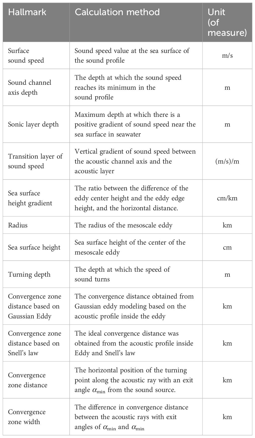
Table 2 Feature calculation method.

Before model training, the extracted features are first analyzed. Taking the anticyclonic eddy as an example, the degree of mutual influence between each element is analyzed using Spearman correlation, considering that the extracted ocean features and the CZ features are not necessarily all linearly correlated. The relative importance of the feature variables is calculated based on the Random Forest algorithm using out-of-bag error (Mitchell, 2011), as shown in Figure 4. The correlation between the distance to the first CZ and each feature is investigated as an example. The contribution of different features to CZ distance prediction is explored. Among the directly extracted marine features, SLD holds the highest relative contribution to prediction, reaching 13.89%. Additionally, the physical information displays higher correlation and features relative importance. For instance, CZ_D (GE), modeling and reconstructing mesoscale eddies by the Gaussian eddy model, demonstrates a high correlation of 0.86 and feature importance of 23.01%. TD shows the highest correlation of 0.90, but its feature importance is only 12.96%, lower than that of CZ_D (S) with a correlation of 0.09 at 15.39%. This might be attributed to the nonlinear correlation between CZ features and oceanic features. In summary, the features selected in this study exhibit a high contribution rate and a relatively uniform distribution in predicting CZ features. The parameters in Table 2 serve as input features in the next model construction.

Figure 4

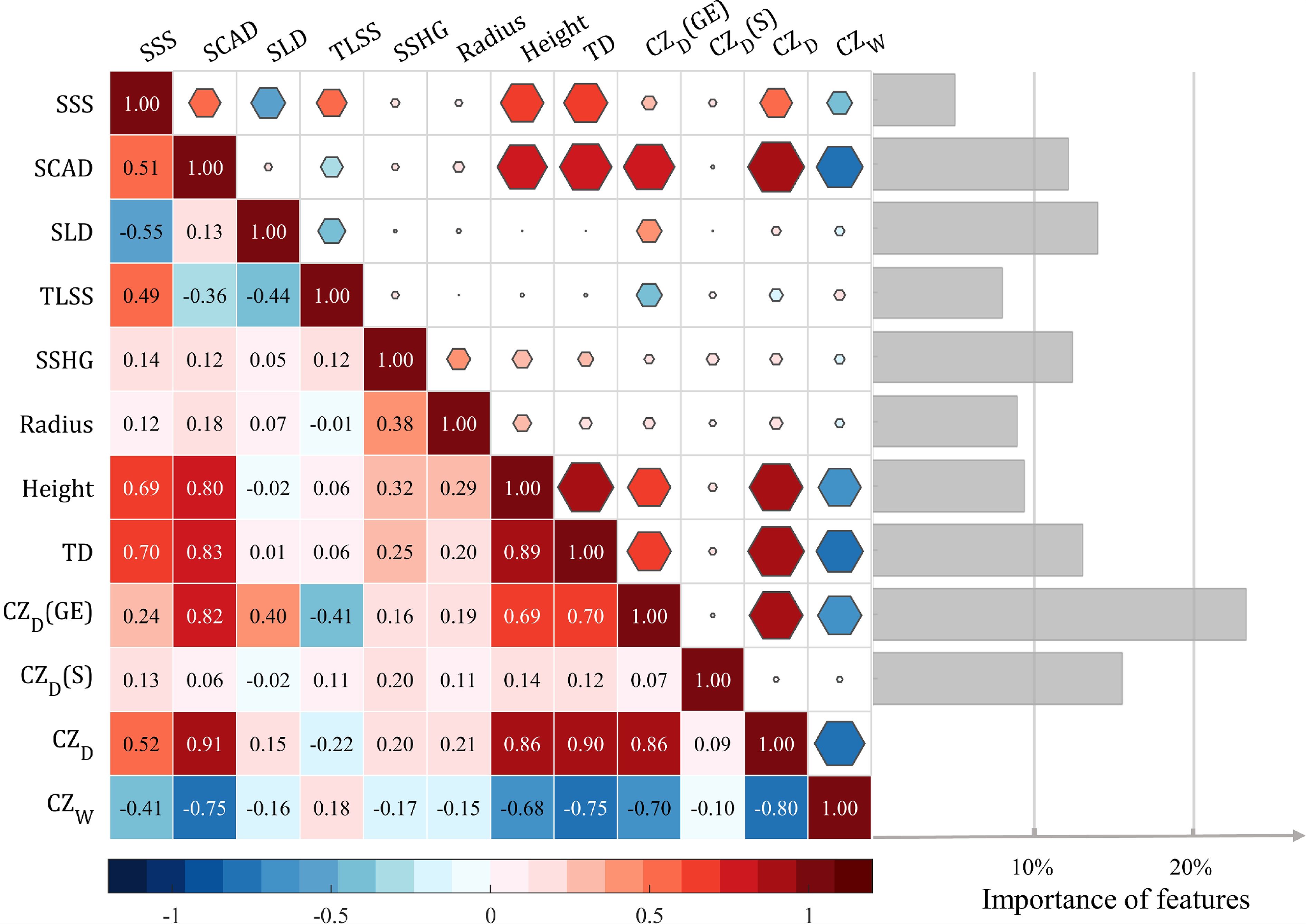
Figure 4 Correlation analysis of oceanic and CZ features extracted from anticyclonic eddies and feature significance based on Random Forest out-of-bag error.

3.2.2 Model evaluation criteria

The model evaluation index uses Mean Absolute Error (MAE) and Accuracy (Equations 16 and 17). A smaller MAE indicates a larger Accuracy, lower dispersion between the model’s predicted value and the real value, and a higher predictive ability of the model.

$\begin{array}{ll}MAE=\frac{1}{n}{\displaystyle \sum _{i=1}^n|y_i-{\widehat{y}}_i|}& (16)\end{array}$

$\begin{array}{ll}Accuracy(mkm)=\frac{{\displaystyle \sum _{i=1}^n{A}_i}}{n}\times 100\%(A_i=\{\begin{array}{l}1,|y_i-{\widehat{y}}_i|\le m\hfill \\ 0,|y_i-{\widehat{y}}_i|>m\hfill \end{array})& (17)\end{array}$

Where y_i represents the real value of CZ prediction, i.e., the value obtained by Bellhop model simulation, and $\widehat{y}$ represents the predicted value, i.e., the features of CZ obtained by the predictive model.

3.3 Model building and training process

After constructing the dataset of input and output features, this study predicts the CZ based on 20 regression algorithms, spanning ensemble approaches (such as SVM and random forest [RF]), deep learning techniques (including CNN and LSTM), and ensemble models (e.g., Multilayer Perceptron–RF [MLP-RF], CNN-GRU). Each algorithm was selected due to its distinctive strengths and potential to offer high predictive accuracy. The relevant algorithms and hyperparameters to be optimized are shown in Table 3. The MLP is optimized using Back Propagation. Ensemble models primarily focus on the integration of deep learning models (including CNN and RNN-based models such as CNN-LSTM, CNN-BiLSTM, and CNN-GRU) as well as the integration of other commonly used simple models (including MLP-RF, MLP-DT, MLP-SVM, and SVM-RF).

Table 3

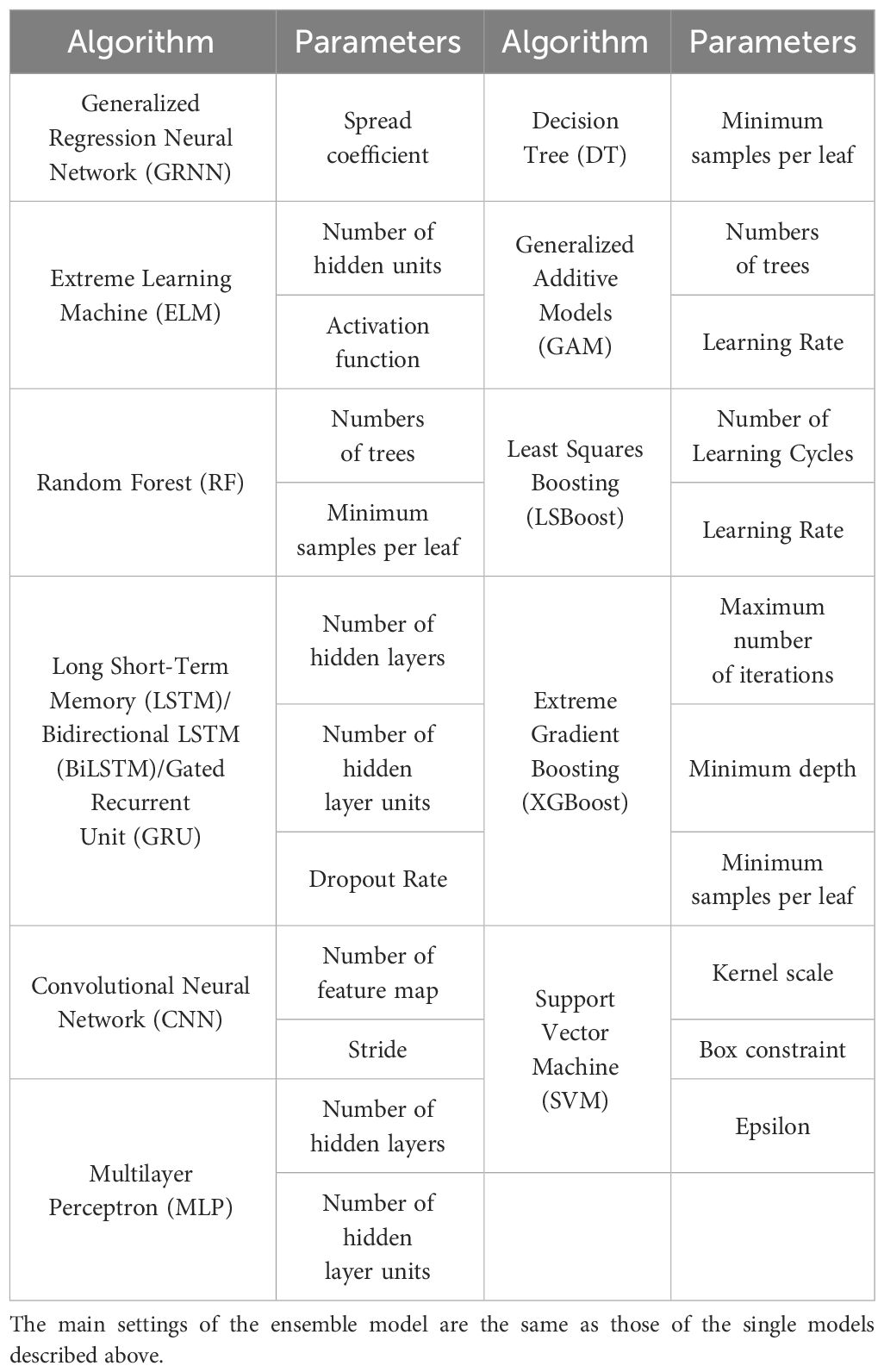
Table 3 Multiple regression model main parameters settings.

The model screening in this subsection is based on the example of the CZ waveguide where the sound source is located in the anticyclonic eddy of study area I and propagates southward. Prior to sample training, the extracted feature dataset is divided into training, validation, and test sets in the ratio of 8:1:1. To improve the convergence speed of the model and the interpretability of the features, the features are firstly standardized. Then, the feature dataset is divided into 10 parts using k-fold cross-validation with approximately 707 samples in each part. Two parts are selected as the validation set and the test set, respectively, and the remaining samples constitute the training set. In each case, the model is trained with the training set, tested with the test set, and the process is repeated 10 times. The average results of these 10 repetitions are taken as the final generalization accuracy evaluation index. The formula used is as follows, where E_i represents the model evaluation index in each training process as shown in Equation 18.

$\begin{array}{ll}E=\frac{1}{10}{\displaystyle \sum _{i=1}^{10}{E}_i}& (18)\end{array}$

Additionally, apart from the 13 single models listed Table 3, there are 7 ensemble models. These ensemble models combine multiple weaker models, adjusting sample weights and model contributions to achieve significantly better generalization performance compared to single models. The process involves creating diverse base models using various sampling or preprocessing techniques on the training data, which are then combined to improve overall prediction accuracy and generalization. The key to this method is optimal integration, determined by a threshold (θ = 0.1). If the model difference (|E₁–E₂|/max(E₁–E₂)) exceeds this threshold, no combination occurs. Otherwise, the model with the smaller error (MAE in this study) is chosen as the final model. When amalgamating the weights of the two models, Equations 19 and 20 are employed, where W denotes the combination weight and y_V represents the prediction result of the two models:

$\begin{array}{ll}\widehat{y}=W_1{y}_{V1}+W_2{y}_{V2}& (19)\end{array}$

$\begin{array}{ll}{W}_1=\frac{E_2}{E_1+E_2},W_2=\frac{E_1}{E_1+E_2}& (20)\end{array}$

To ensure reasonable settings for each hyperparameters in Table 3 during model training, this study uses the SSA. This algorithm represents a new type of swarm intelligence optimization algorithm inspired by the foraging and antipredation behaviors of sparrows. The SSA simulates the strategies and behaviors of sparrows during foraging. It effectively explores the solution space and aims to seek the optimal or near-optimal solution. Known for its global search ability and convergence, SSA is applicable for solving various optimization problems (Xue and Shen, 2020).

During the training process, this study assesses the prediction effect of two cases: machine learning with physical information inputs [TD, CZ_D (GE), and CZ_D (S)] and machine learning without physical information inputs, and the prediction accuracy is assessed as shown in Figure 5, after training and evaluating each model. RF regression is found to be the optimal performer in prediction with an Accuracy(1km) of more than 85% for both its single and ensemble models, followed by physical information and machine learning, which shows great potential in the prediction of CZ features. The model achieves a maximum reduction of 0.82 km in MAE compared to the case of no physical information input by incorporating an appropriate physical model. When there is limited data on the marine environment, the Accuracy (1km) is improved ranging from 2.80 to 11.92%. Taking all these considerations into account, the ensemble model with the highest accuracy, MLP-RF, was identified as the machine learning model to perform the prediction of CZ features in the mesoscale eddy environment in this study, with an MAE of 0.93 km and an Accuracy(1km) of 87.36% after K-fold cross-validation.

Figure 5

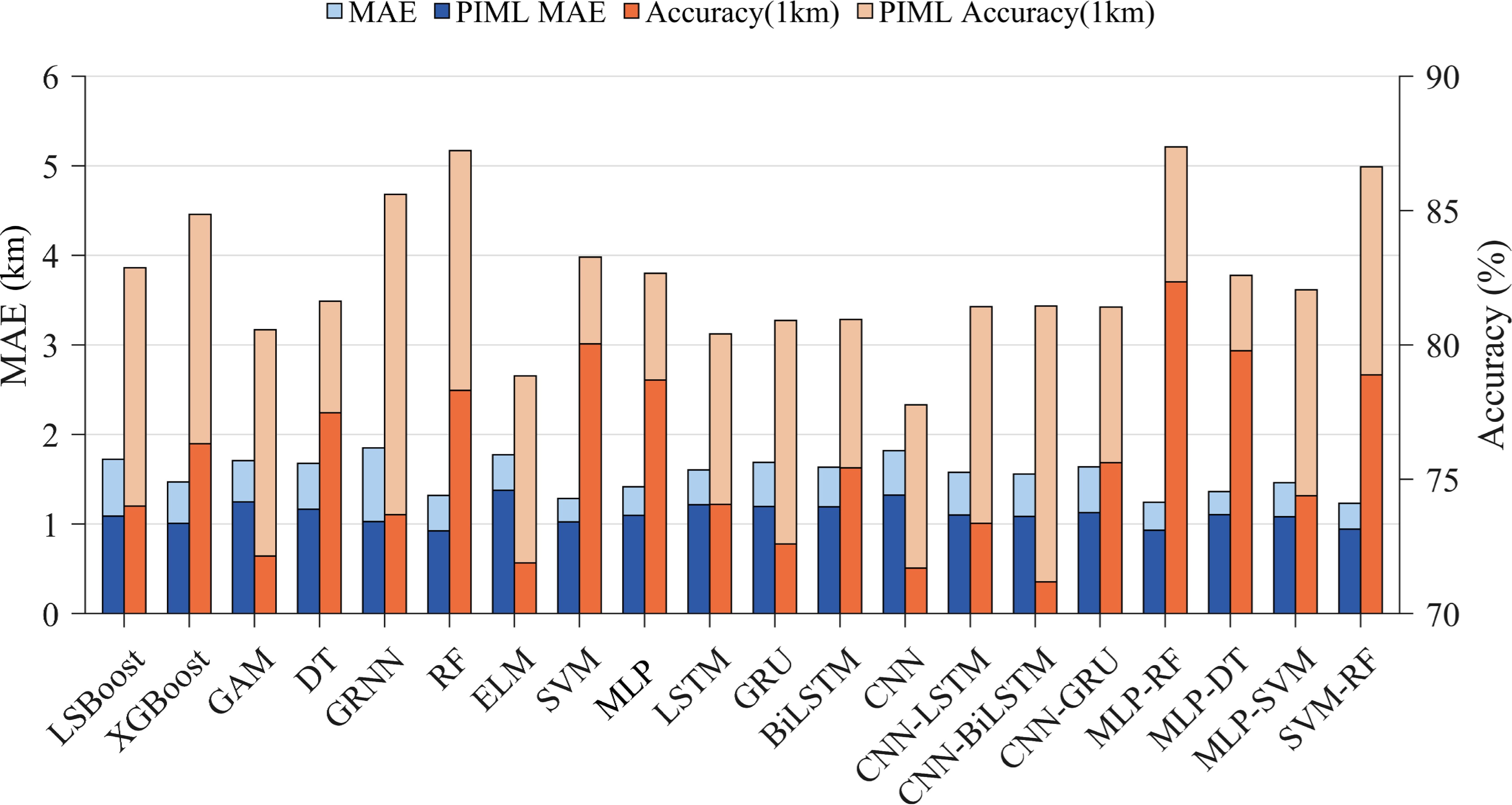
Figure 5 Comparison of predictive models for CZ_D using PIML and no physical information input machine learning algorithms: focus on anticyclonic eddies in research area I.

4 Model prediction results

4.1 Two-dimensional prediction results

In this section, the CZ features of the cyclonic and anticyclonic eddies in the Study Area I are initially predicted. Based on the optimal predictive model obtained in the previous section—using extracted ocean features to predict the distance to the CZ— this subsection still considers the sound source located in the center of the eddy propagating southward as an example. The trend of the distance and width of the first CZ can be accurately predicted by relying solely on one acoustic contour line within the center of the eddy and the eddy’s features. Figure 6 illustrates the line plots of the predicted results of the CZ distance and width within Study Area I (taking the first three hundred predictions as an example), along with the scatter density plots. The MLP-RF-based CZ predictive model can effectively predict the CZ features using mesoscale eddy features under limited data. The machine learning-based prediction method in the line plot accurately predicts the CZ trends, and the scatter points in the scatter plot are closely distributed near the 1:1 line. The width of the CZ is calculated from two acoustic lines emitted from the minimum and maximum outgoing angles, which introduces more uncertainties and errors than the distance calculation from one acoustic line. Consequently, the accuracy of the width prediction is slightly lower than that of the distance. The Accuracy(1km) of the CZ distance prediction in the anticyclonic eddy environment is 86.88%, the MAE is 0.92 km, the Accuracy(1km) of the CZ width prediction is 79.49%, and the MAE is 1.49 km; the Accuracy(1km) of the CZ distance prediction in the cyclonic eddy environment is 91.40%, the MAE is 0.69 km, and the predicted Accuracy(1km) of the CZ width is 72.23% with a MAE of 1.85 km.

Figure 6

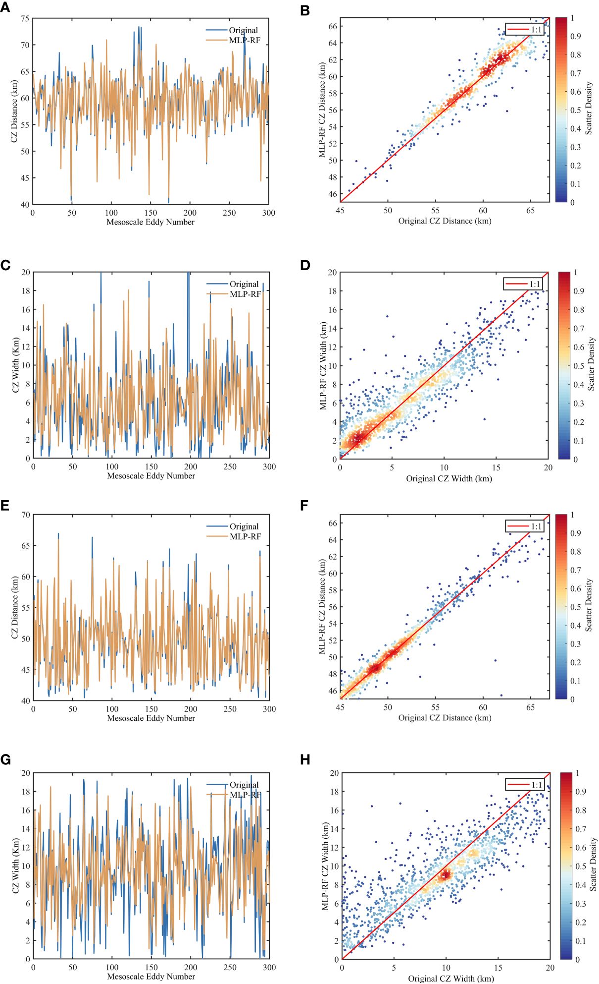
Figure 6 CZ prediction line and scatter density plots in two-dimensional mesoscale eddy environments: (A) anticyclonic eddy CZ distance prediction line plot; (B) anticyclonic eddy CZ distance prediction scatter density plot; (C) anticyclonic eddy CZ width prediction line plot; (D) anticyclonic eddy CZ width prediction scatter density plot; (E) cyclonic eddy CZ distance prediction line plot; (F) cyclonic eddy CZ distance prediction scatter density plot; (G) cyclonic eddy CZ width prediction line plot; (H) cyclonic eddy CZ width prediction scatter density plot.

4.2 Three-dimensional prediction results

CZ waveguides facilitate long-distance detection and communication. This study extends the previous research to investigate the first three CZ within a mesoscale eddy environment. To simplify the prediction process, the first three CZs are predicted in four directions: east, south, west, and north, for the sound source positioned at the center of the eddy. The predicted distances of the CZs in each direction are averaged and superimposed on the averaged predicted widths. These predictions are then compared with the 3D underwater acoustic propagation results obtained by simulating high-resolution mesoscale eddy ocean data through Bellhop. Figure 7 displays the comparison maps using the anticyclonic eddy on the first day of each month in 2021 as an example. The evaluation focuses on the prediction results in different directions. The TL represents the loss of acoustic energy from the source emissions during propagation, which is derived from Bellhop simulations. The concentric area in Figure 7 with a lower TL corresponds to the CZ.

Figure 7

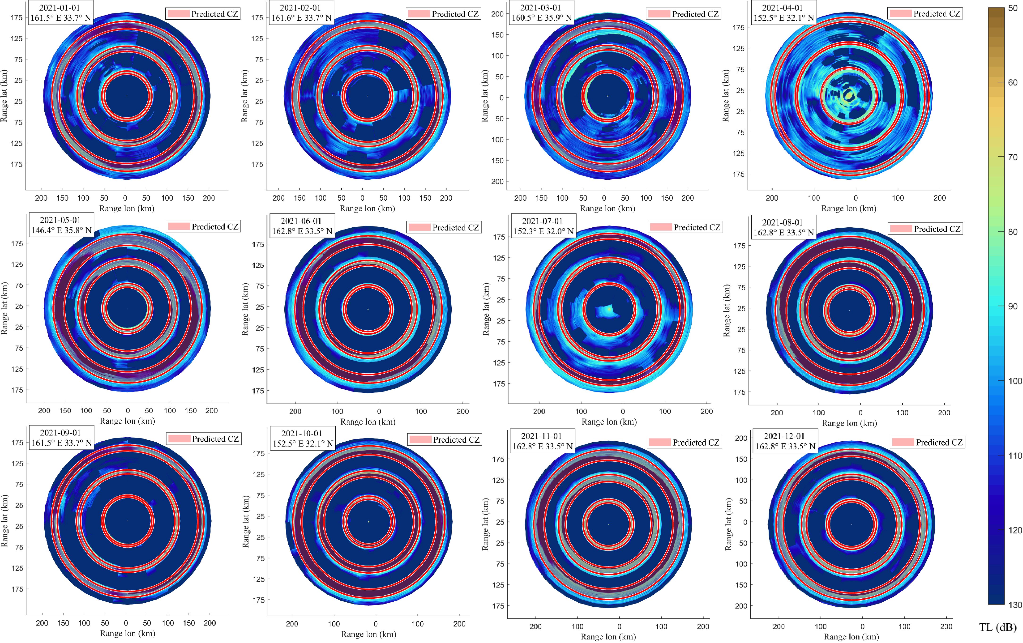
Figure 7 The schematic diagram of simulation of mesoscale eddy transmission loss and machine learning-based CZ prediction results in the KE region in 2021 (illustrating one mesoscale eddy per month, with the annular area of low transmission loss as the CZ).

In this study, the effectiveness of feature prediction for the first three CZs in the anticyclonic eddy environment and the cyclonic eddy environment was evaluated (Tables 4 and 5). In the anticyclonic eddy environment, predictions of distance and width of the first CZ shows high accuracy in all directions, with MAE between 0.99 and 1.46 km and an accuracy (within 3 km) of more than 95%. The prediction accuracy gradually decreases with the increase of the CZ number, especially when the MAE of the third CZ distance and width rises to 3.63–4.57 km, and the accuracy decreases from 76.78% to 82.33%. In the cyclonic eddy environment, the MAE for predicting the distance and width of the first CZ range from 0.67 to 2.38 km, and the accuracy (within 3 km) stays at 93.35% to 99.23%. However, the difficulty of prediction significantly increases with the number of CZs. In the third CZ, the MAE for distance and width increases to 2.74–6.51 km, while accuracy decreases from 67.88% to 89.59%.

Table 4

Table 4 Evaluation of predictive performance for CZ features in the anticyclonic eddy environment.

Table 5

Table 5 Evaluation of predictive performance for CZ features in the cyclonic eddy environment.

In summary, the model demonstrates the initial feasibility of using limited data within mesoscale eddy ocean environment to predict CZ features. It exhibits considerably high accuracy, particularly in predicting the first CZ. However, as the prediction span extends (such as in the case of the third CZ, typically around 180 km), relying solely on mesoscale eddy features within a radius of approximately 100 km for predicting these initial three CZs inevitably introduces errors. Nevertheless, the current model showcases adaptability and robustness across diverse mesoscale eddy environments, maintaining an overall acceptable prediction error. These evaluation results underscore the model’s potential for accurate predictions within highly dynamic environments, laying a strong foundation for future predictions under more complex oceanographic conditions.

5 Validation and generalization of the model

5.1 Validation of study area II

Study Area II is a region of OE where mesoscale eddies have a significant impact on the oceanographic properties of the region (Yang et al., 2022). This region exhibits different dynamics compared to the KE region. In this study, the pair of mesoscale eddies in this region is used as a comparison, and the features of the CZ in the mesoscale eddy environment in this region are directly predicted using the model trained in the previous section. By subtracting the predictions from the full-element ocean simulation results, the prediction errors in the four directions for the first three CZs are obtained, and box plot as well as line plots of the average prediction errors are plotted accordingly (see Figure 8). The whisker length in the box plot was determined by extending to 1.5 times the interquartile range beyond the box, which is defined by the first and third quartiles. Data points falling more than 1.5 times the interquartile range above the third quartile or below the first quartile were identified as outliers, and whiskers extended to the furthest non-outlier data points.

Figure 8

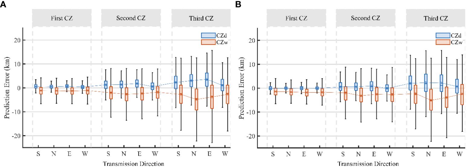
Figure 8 Box plot of prediction errors for mesoscale eddy CZs in the oceanic area of the OE: (A) anticyclonic eddies; (B) cyclonic eddies (where S, N, E, and W represent the propagation of acoustic rays emitted from the sound source located at the center of the eddies to the south, north, east, and west, respectively).

Consistent with the findings in the previous section, the prediction errors between different CZs exhibit significant variability. After analyzing 12 sets of data for both types of eddies, it is observed that the distribution of prediction errors exhibits a high degree of consistency. The prediction errors in the first CZ are significantly lower than those in the other two regions, exhibiting good agreement in their mean and median values. For the anticyclonic eddy, the median prediction error for the distance from the first CZ is approximately 0.5 km. The interquartile range predominantly spans between 0 and 1 km, with the whisker line endpoints roughly between -2 and 3 km. Concerning the cyclonic eddy, the median prediction error is less than 0.1 km, with an interquartile range predominantly between -0.5 and 0.5 km, and whisker line endpoints are roughly between -2.5 and 2.5 km. The prediction errors for the width of the first CZ are similar for both eddies, with a median of approximately -1 km, an interquartile range of -2.5 km to 0.5 km, and whisker line endpoints roughly between -6 and 4 km. In contrast, the prediction errors of the second and third CZs are relatively high, and the predicted values of the CZ distances are still smaller than the simulated values, with the interquartile ranges of the second CZ predominantly between -1 and 2 km, and the interquartile ranges of the third CZ predominantly between -1 and 5 km. The predicted values of cluster width are still larger than the simulated values, the second cluster quartile range is predominantly around -5 km–0 km, and the third cluster quartile range is predominantly around -7 km–1 km.

The comparison of prediction errors among the four directions suggests significant differences in the four directions eastward, southward, westward, and northward. Specifically, the prediction error of the CZ propagating to the west is the smallest, indicating a stronger prediction ability of the model in that direction. The relatively higher prediction error for the CZ propagating northward may be related to the fact that the Study Area II is located at the southern end of the OE, and the changes of oceanic elements are more complicated in this direction, thus negatively affecting the prediction accuracy of the model.

In summary, based on the analysis results of the grouped box plot, the prediction error of the CZs in the mesoscale environment varies across CZ and directions. The prediction error increases with the prediction span of the CZ, with lower prediction error in the first CZ and higher prediction error in the second and third CZ. The prediction errors are lowest for CZ propagating westward and relatively high for those propagating northward. These results suggest that the prediction errors of raw CZ in mesoscale eddy environments are related to the complexity and stability of the marine environment.

5.2 Validation of underwater acoustic propagation simulation based on in-situ data

JCOPE2M assimilates various in-situ data, including Argo and sea surface height data. As stated in Section 2.1.2, the mesoscale eddies used in this study are features that are simultaneously present in the reanalysis data and sea surface height data. This study considers these eddies to be real.

Therefore, to further verify whether the predictive model proposed in this study can utilize limited in-situ observational data to predict the features of sound CZ in the mesoscale eddy environment, seven input features from the previous model are extracted using Argo floats. This extraction excludes the height, radius, and horizontal gradient of the sea surface. The selection criteria for mesoscale eddies and Argo floats are as follows: using the distribution data of mesoscale eddies provided by AVISO, this study selects mesoscale eddies with Argo float data available within 3° of the eddy center for three days before and after the existence of the eddy as validation samples for this section. The features of the remaining mesoscale eddies without Argo float data are utilized as the training dataset for the model.

The distribution of Argo and its latitude distribution utilized in this study are initially plotted, as depicted in Figure 9. These distributions exhibit similarities to the mesoscale eddy distribution identified in Figure 2, validating them as representative mesoscale eddies. In the evaluation, the prediction performance of anticyclonic eddies shows higher accuracy, especially in the first CZ (Tables 6 and 7). Specifically, the MAE of the first CZ distance ranges between 2.36 to 2.50 km, with accuracy ranging from 81.85% to 84.24%; while the MAE of width ranges between 2.00 to 2.15 km, with accuracy ranging from 90.65% to 91.85%. In comparison, the prediction performance of cyclonic eddies is slightly inferior, with MAE of the first CZ distance ranging from 2.66 to 2.87 km, and accuracy ranging from 77.26% to 80.99%; and MAE of width ranging from 2.88 to 3.10 km, with accuracy ranging from 80.58% to 84.51%. In width prediction, the accuracy of both anticyclonic and cyclonic eddies is generally higher than that of distance prediction, possibly due to the smaller scale of width parameters, exhibiting higher accuracy under the same 3 km precision evaluation criteria.

Figure 9

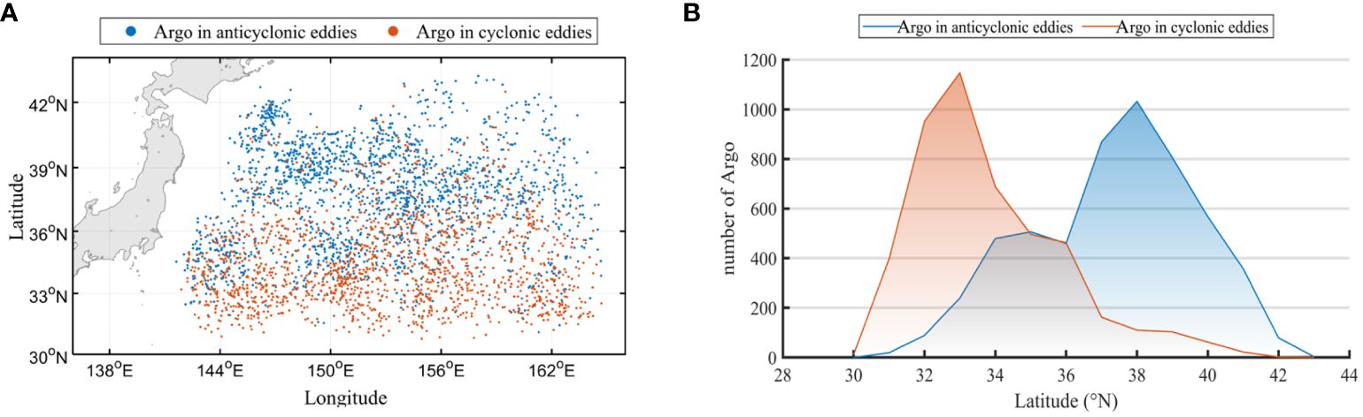
Figure 9 Distribution of Argo screened for CZ prediction in this study: (A) Argo location distribution map; (B) Argo distribution with latitude.

Table 6

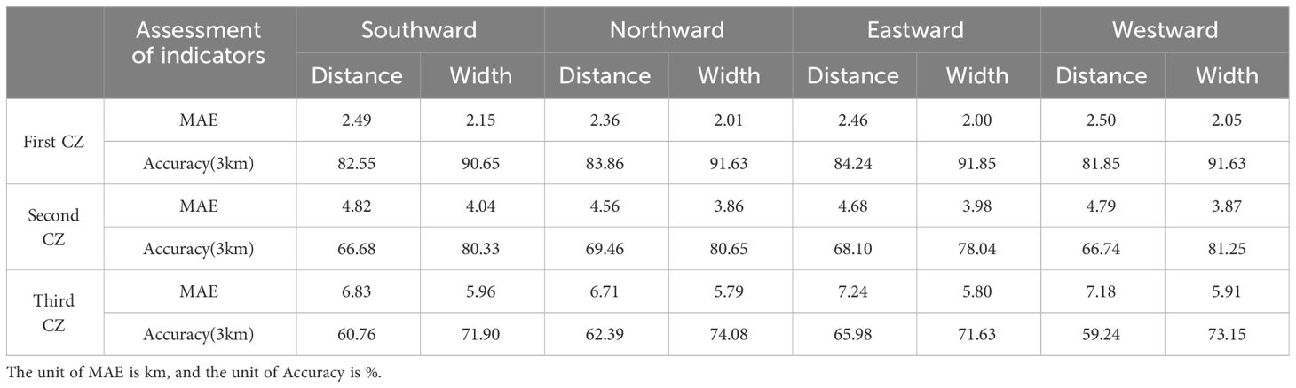
Table 6 Assessment of the effectiveness of anticyclonic eddy prediction based on Argo data.

Table 7

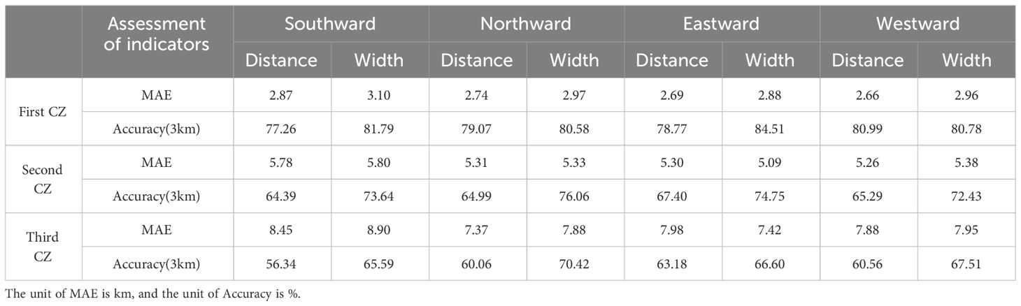
Table 7 Assessment of the effectiveness of cyclonic eddy prediction based on Argo data.

As the span of the CZ widens, the prediction accuracy for both types of eddies decreases. In predicting the third CZ distance, the MAE values for anticyclonic eddies increase to 6.71–7.24 km and the accuracy decreases to 59.24%–65.98%. In contrast, the MAE values of cyclonic eddies increase to 7.37 km–8.45 km and the accuracy decreases to 56.34%–63.18%. This trend suggests that more distant CZ pose greater challenges for predictive modeling, potentially due to the increased complexity of ocean dynamics associated with a wider CZ span. Overall, anticyclonic eddies tend to be better predicted than cyclonic eddies. However, both exhibit significantly lower prediction accuracies than the features extracted via JCOPE2M. For practical application, incorporating more Argo float-extracted features and their corresponding 3D mesoscale eddy structures into the training and test sets could offer a means to derive the acoustic propagation properties of mesoscale eddies solely from data returned by Argo floats and satellite altimeters.

6 Conclusion

In this study, a new method is proposed to identify oceanic mesoscale eddies based on the convex hull ratio. High-resolution reanalysis data and an AVISO-based mesoscale eddy dataset are utilized to screen tens of thousands of mesoscale eddies exhibiting significant features in both datasets. Key features of these eddies and CZs are extracted using physical modeling and acoustic line tracking techniques. Subsequently, a robust prediction dataset is established based on these extracted features. Throughout the model construction process, K-fold cross-validation and SSA are employed to select the most accurate algorithms from a pool of 20 machine learning algorithms. This leads to the formation of a mesoscale eddy CZ predictive model that demonstrates high accuracy and strong generalization ability, particularly when dealing with limited data.

The findings of this study indicate the effectiveness of the proposed identification method in screening mesoscale eddies with eddy features within the KE region. The CZ predictive model, constructed using the MLP-RF algorithm, performs impressively in accuracy assessment, achieving an MAE of 0.93 km and an accuracy rate (1km) of 87.36%. Moreover, the integration of physical information into machine learning exhibits significant potential in predicting CZ features. When marine environmental data are limited, incorporating suitable physical information [such as TD, CZ_D (GE), and CZ_D (S)] contributes to a maximum reduction of 0.82 km in MAE and an improvement in Accuracy (1km) by 2.80% to 11.92% compared to the model without physical information input.

On this basis, the effectiveness of feature prediction for the first three CZs in both the anticyclonic and cyclonic eddy environments was further evaluated. The predictions for distance and width of the first CZ in both eddy types demonstrate high accuracy in all directions, with MAE of approximately 1.00 km and accuracy (within 3 km) exceeding 95%. However, as the sequence number of the CZ increases, the prediction accuracy gradually diminishes. Specifically, the MAE for distance and width of the third CZ rises to approximately 4 km, with an accuracy decrease to 70%–80%. This result implies an increased challenge for the model when predicting more distant CZs. This challenge is associated with the number of features inputs of mesoscale eddies and the complexity of ocean dynamics.

To verify the generalizability and practical value of the model, this study validates the predictive model by cross-validating the sea area and Argo float data. This validation approach exhibits excellent performance in assessing the prediction accuracy of CZ features. In the future, considering more Argo float data and constructing a dataset closely resembling the actual mesoscale eddy environment through the 3D mesoscale eddy structure of the in-situ information can further enhance the predictive capability of the model.

The present study focuses on predicting acoustic CZs in mesoscale eddy environments in the Kuroshio‐Oyashio Extension region with limited data. Utilizing a wide range of high-resolution reanalysis data and screening satellite altimeters as an alternative to in-situ data are representative techniques to a certain extent. However, it still has a gap in reflecting the actual environment of mesoscale eddies. Several challenges persist. Firstly, it remains challenging to achieve real-time acoustic parameter prediction of the mesoscale environment with maximum accuracy while building as few submerged or floating arrays as possible. Secondly, resolving the scarcity of in-situ mesoscale eddy data and acoustic CZ observations during model construction is crucial. It is hoped that the methodology and insights presented in this study will inspire further investigations and contribute to the ongoing advancements in the field of ocean acoustics, particularly in establishing robust and globally applicable predictive models for mesoscale eddy parameters.

Data availability statement

The original contributions presented in the study are included in the article/supplementary material. Further inquiries can be directed to the corresponding author.

Author contributions

WX: Investigation, Software, Writing – original draft, Writing – review & editing. LZ: Formal analysis, Funding acquisition, Investigation, Writing – review & editing. ML: Writing – original draft, Data curation, Validation, Funding acquisition, Writing – review & editing. XM: Data curation, Resources, Validation, Visualization, Writing – original draft. HW: Formal analysis, Funding acquisition, Software, Writing – review & editing.

Funding

The author(s) declare financial support was received for the research, authorship, and/or publication of this article. This project was funded by the North Pacific Deep Sound Zoning Study (DJYSYF2020-008) and the Scientific Research and Development Fund of Dalian Naval Academy.

Acknowledgments

We extend our gratitude to Japan Agency for Marine-Earth Science and Technology for their support in providing the JCOPE2M data (https://www.jamstec.go.jp/jcope/htdocs/distribution/index.html), to NCEI for granting access to the bathymetric data ETOPO (https://www.ncei.noaa.gov/products/etopo-global-relief-model). Our thanks also go to AVISO for sharing the mesoscale eddy dataset (https://www.aviso.altimetry.fr/en/data/products/value-added-products/global-mesoscale-eddy-trajectory-product.html), and to the International Argo Program (IAP) for providing float data (https://argo.ucsd.edu/). We express our appreciation to Mr. Ruochao Zhang of JAMEST for his valuable assistance in data processing. Additionally, we acknowledge the contributions of other scholars and organizations that played a role in our research process. We are especially grateful to the reviewers for their thorough and professional insights, which significantly enhanced the quality of this manuscript.

Conflict of interest

The authors declare that the research was conducted in the absence of any commercial or financial relationships that could be construed as a potential conflict of interest.

Publisher’s note

All claims expressed in this article are solely those of the authors and do not necessarily represent those of their affiliated organizations, or those of the publisher, the editors and the reviewers. Any product that may be evaluated in this article, or claim that may be made by its manufacturer, is not guaranteed or endorsed by the publisher.

References

Akulichev V. A., Bugaeva L. K, Morgunov Yu. N, Solovjev A. A. (2012). Influence of mesoscale eddies and frontal zones on sound propagation at the Northwest Pacific Ocean. J. Acoust Soc. America 131, 3354–3354. doi: 10.1121/1.4708575

CrossRef Full Text | Google Scholar

Amante C., Eakins B. W. (2009). ETOPO1 arc-minute global relief model: procedures, data sources and analysis. NOAA Tech. Memorandum NESDIS NGDC 24, 1–19. doi: 10.7289/V5C8276M

CrossRef Full Text | Google Scholar

Barone B., Church M. J., Dugenne M., Hawco N. J., Jahn O., White A. E., et al. (2021). Biogeochemical dynamics in adjacent mesoscale eddies of opposite polarity. Global Biogeochem Cycles 36, e2021GB007115. doi: 10.1002/essoar.10507480.1

CrossRef Full Text | Google Scholar

Chang Y.-L. K., Miyazawa Y., Béguer-Pon M., Han Y. S., Ohashi K., Sheng J. (2018). Physical and biological roles of mesoscale eddies in Japanese eel larvae dispersal in the western North Pacific Ocean. Sci. Rep. 8, 1–11. doi: 10.1038/s41598-018-23392-5

PubMed Abstract | CrossRef Full Text | Google Scholar

Chang Y. L., Miyazawa Y., Guo X. (2015). Effects of the STCC eddies on the Kuroshio based on the 20-year JCOPE2 reanalysis results. Prog. Oceanogr 135, 64–76. doi: 10.1016/j.pocean.2015.04.006

CrossRef Full Text | Google Scholar

Chelton D. B., Schlax M. G., Samelson R. M. (2011). Global observations of nonlinear mesoscale eddies. Prog. Oceanogr 91, 167–216. doi: 10.1016/j.pocean.2011.01.002

CrossRef Full Text | Google Scholar

Chen W., Zhang Y., Liu Y., Wu Y., Zhang Y., Ren K. (2022). Observation of a mesoscale warm eddy impacts acoustic propagation in the slope of the South China Sea. Front. Mar. Sci. 9. doi: 10.3389/fmars.2022.1086799

PubMed Abstract | CrossRef Full Text | Google Scholar

Chen X., Hong M., Zhu W., Mao K., Ge J., Bao S. (2019). The analysis of acoustic propagation characteristic affected by mesoscale cold-core vortex based on the UMPE model. Acoust Aust. 47, 33–49. doi: 10.1007/s40857-019-00149-2

CrossRef Full Text | Google Scholar

Doan V.-S., Huynh-The T., Kim D.-S. (2020). Underwater acoustic target classification based on dense convolutional neural network. IEEE Geosci. Remote Sens. Lett. 19, 1–5. doi: 10.1109/LGRS.2020.3029584

CrossRef Full Text | Google Scholar

Duo Z., Wang W., Wang H. (2019). Oceanic mesoscale eddy detection method based on deep learning. Remote Sens. 11, 1921. doi: 10.3390/rs11161921

CrossRef Full Text | Google Scholar

Etter P. C. (2013). Underwater Acoustic Modeling and Simulation, Fourth Edition (London: CRC Press).

Google Scholar

Hamilton E. L. (1980). Geoacoustic modeling of the sea floor. J. Acoust Soc. America 68, 1313–1340. doi: 10.1121/1.385100

CrossRef Full Text | Google Scholar

He Y., Feng M., Xie J., He Q., Liu J., Xu J., et al. (2021). Revisit the vertical structure of the eddies and eddy-induced transport in the Leeuwin current system. J. Geophys Res. 126, e2020JC016556. doi: 10.1029/2020JC016556

CrossRef Full Text | Google Scholar

Itoh S., Yasuda I. (2010). Characteristics of mesoscale eddies in the Kuroshio-Oyashio extension region detected from the distribution of the sea surface height anomaly. J. Phys. Oceanogr 40, 1018–1034. doi: 10.1175/2009JPO4265.1

CrossRef Full Text | Google Scholar

Jiang M., Zhu Z. (2022). The role of artificial intelligence algorithms in marine scientific research. Front. Mar. Sci 9, 920994. doi: 10.3389/fmars.2022.920994

CrossRef Full Text | Google Scholar

Liu Z. J., Nakamura H., Zhu X.-H., Nishina A., Guo X., Dong M. (2019). Tempo-spatial variations of the Kuroshio current in the Tokara Strait based on long-term ferryboat ADCP data. J. Geophys Res: Oceans 124, 6030–6049. doi: 10.1029/2018JC014771

CrossRef Full Text | Google Scholar

Liu J., Piao S., Gong L., Zhang M., Guo Y., Zhang S. (2021). The effect of mesoscale eddy on the characteristic of sound propagation. J. Mar. Sci. Eng. 9, 787. doi: 10.3390/jmse9080787

CrossRef Full Text | Google Scholar

Mackenzie K. V. (1981). Nine-term equation for sound speed in the oceans. J. Acoust Soc. America 70, 807–812. doi: 10.1121/1.386920

CrossRef Full Text | Google Scholar

Mahpeykar O., Larki A. A., Nasab M. A. (2022). The effect of cold eddy on acoustic propagation (Case study: eddy in the Persian Gulf). Arch. Acoust 47, 413–423. doi: 10.24425/aoa.2022.142015

CrossRef Full Text | Google Scholar

Meng C., Seo S., Gao D., Griesemer S., Liu Y. (2022). When physics meets machine learning: A survey of physics-informed machine learning. ArXiv, abs/2203.16797. doi: 10.48550/arXiv.2203.16797

CrossRef Full Text | Google Scholar

Mitchell M. W. (2011). Bias of the random forest out-of-bag (OOB) error for certain input parameters. Open J. Stat 1, 205–211. doi: 10.4236/ojs.2011.13024

CrossRef Full Text | Google Scholar

Miyazawa Y., Varlamov S. M., Miyama T., Guo X., Hihara T., Kiyomatsu K., et al. (2017). Assimilation of high-resolution sea surface temperature data into an operational nowcast/forecast system around Japan using a multi-scale three-dimensional variational scheme. Ocean Dyn 67, 713–728. doi: 10.1007/s10236-017-1056-1

CrossRef Full Text | Google Scholar

Miyazawa Y., Kuwano-Yoshida A., Doi T., Nishikawa H., Narazaki T., Fukuoka T., et al. (2019). Temperature profiling measurements by sea turtles improve ocean state estimation in the Kuroshio-Oyashio Confluence region. Ocean Dyn 69, 267–282. doi: 10.1007/s10236-018-1238-5

CrossRef Full Text | Google Scholar

Munk W. H. (1974). Sound channel in an exponentially stratified ocean, with application to SOFAR. J. Acoust Soc. America 55, 220–226. doi: 10.1121/1.1914492

CrossRef Full Text | Google Scholar

Porter M. B. (2011). The bellhop manual and user’s guide: Preliminary draft. Heat, Light, and Sound Research, Inc., La Jolla, CA, USA. Tech Rep. 260.

Google Scholar

Roemmich D. H., Johnson G. C., Riser S., Davis R., Gilson J., Owens W. B., et al. (2009). The Argo Program: observing the global ocean with profiling floats. Oceanography 22, 34–43. doi: 10.5670/oceanog.2009.36

CrossRef Full Text | Google Scholar

Sadaiappan B., Balakrishnan P., Vishal C. R., Vijayan N. T., Subramanian M., Gauns M. U. (2022). Applications of machine learning in chemical and biological oceanography. ACS Omega 8, 15831–15853. doi: 10.1021/acsomega.2c06441

CrossRef Full Text | Google Scholar

Scharffenberg M. G., Stammer D. (2010). Seasonal variations of the large-scale geostrophic flow field and eddy kinetic energy inferred from the TOPEX/Poseidon and Jason-1 tandem mission data. J. Geophys Res. 115, C02008. doi: 10.1029/2008JC005242

CrossRef Full Text | Google Scholar

Taguchi B., Qiu B., Nonaka M., Sasaki H., Xie S. P., Schneider N., et al. (2010). Decadal variability of the Kuroshio Extension: mesoscale eddies and recirculations. Ocean Dyn 60, 673–691. doi: 10.1007/s10236-010-0295-1

CrossRef Full Text | Google Scholar

Wang X., Wang H., Liu D., Wang W. (2020). The prediction of oceanic mesoscale eddy properties and propagation trajectories based on machine learning. Water 12, 2521. doi: 10.3390/w12092521

CrossRef Full Text | Google Scholar

Xiao R., Lei F., Zhu H., Chen C., Xue Y. (2021). Influence of mesoscale vortex on underwater low-frequency sound propagation. J. Physics: Conf. Ser. 1739, 12018. doi: 10.1088/1742-6596/1739/1/012018

CrossRef Full Text | Google Scholar

Xiao Y., Li Z., Sabra K. G. (2018). Effect of mesoscale eddies on deep-water sound propagation. J. Acoust Soc. America 143, 1873–1874. doi: 10.1121/1.5036149

CrossRef Full Text | Google Scholar

Xue J., Shen B. (2020). A novel swarm intelligence optimization approach: sparrow search algorithm. Syst. Sci. Control Eng. 8, 22–34. doi: 10.1080/21642583.2019.1708830

CrossRef Full Text | Google Scholar

Yang K., Lu Y., Xue R., Sun Q. (2018). Transmission characteristics of convergence zone in deep-sea slope. Appl. Acoust 139, 222–228. doi: 10.1016/j.apacoust.2018.05.004

CrossRef Full Text | Google Scholar

Yang H., Lee K., Choo Y., Kim K. (2020). Underwater acoustic research trends with machine learning: general background. J. Ocean Eng. Technol. 34, 147–154. doi: 10.26748/KSOE.2020.015

CrossRef Full Text | Google Scholar

Yang H., Zhu R., Chen Z., Li J., Wu L. (2022). Temperature variability and eddy-flow interaction in the south of Oyashio Extension. J. Geophys Res: Oceans 127, e2022JC019051. doi: 10.1029/2022JC019051

CrossRef Full Text | Google Scholar

Yao H., Ma C., Jing Z., Zhang Z. (2023). On the vertical structure of mesoscale eddies in the Kuroshio-Oyashio extension. Geophys Res. Lett. 50, e2023GL105642. doi: 10.1029/2023GL105642

CrossRef Full Text | Google Scholar

Zhai X., Yang Z. (2022). Eddy-induced meridional transport variability at ocean western boundary. Ocean Model 171, 101960. doi: 10.1016/j.ocemod.2022.101960

CrossRef Full Text | Google Scholar

Zhao J., Wang F., Gao S., Hou Y., Liu K. (2021). Mass transport of a mesoscale eddy in the South China Sea identified by a simulated passive tracer. J. Oceanol Limnol 40, 389–412. doi: 10.1007/s00343-021-1069-y

CrossRef Full Text | Google Scholar