Improved sea surface salinity data for the Arctic Ocean derived from SMAP satellite data using machine learning approaches

Salinity is among the key climate characteristics of the World Ocean. During the last 15 years, sea surface salinity (SSS) is measured using satellite passive microwave sensors. Standard retrieving SSS algorithms from remote sensing data were developed and verified for the most typical temperature and salinity values of the World Ocean. However, they have far lower accuracy for the Arctic Ocean, especially its shelf areas, which are influenced by large river runoff and have low typical temperature and salinity values. In this study, an improved algorithm has been developed to retrieve SSS in the Arctic Ocean during ice-free season, based on Soil Moisture Active Passive (SMAP) mission data, and using machine learning approaches. Extensive database of in situ salinity measurements in the Russian Arctic seas collected during multiple field surveys is applied to train and validate the machine learning models. The error in SSS retrieval of the developed algorithm compared to the standard algorithm reduced from 3.15 to 2.15 psu, and the correlation with in situ data increased from 0.82 to 0.90. The obtained daily SSS fields are important to improve accurate assessment of spatial and temporal variability of large river plumes in the Arctic Ocean.

1 Introduction

Sea salinity is a crucial factor for understanding physical processes in the World Ocean and is recognized as one of the key climate variables (Durack et al., 2016). Sea salinity affects sea density, heat capacity, and other characteristics of seawater. Salinity together with temperature determine the global system of density currents in the World Ocean (Le Vine, 2019; Le Vine and Dinnat, 2020). Sea salinity is influenced by multiple processes including precipitation and evaporation, continental freshwater runoff, ice formation and melting. As a result, salinity measurements provide information about internal ocean water structure, as well as ocean–atmosphere and land–ocean interactions (Horner-Devine et al., 2015; Durack et al., 2016; Dinnat et al., 2019).

During the last 15 years, remote sensing measurements are actively used to gather sea surface salinity (SSS). The Soil Moisture and Ocean Salinity (SMOS) mission (Kerr et al., 2010) (launched in 2009), the Aquarius mission (Le Vine et al., 2007) (launched in 2011), and the Soil Moisture Active Passive (SMAP) mission (Entekhabi et al., 2010) (launched in 2015) provide sea salinity data. L–band (1.4 GHz) microwave sensors, installed on these satellites, allow to retrieve SSS values from microwave radiation data (Boutin et al., 2018; Dinnat et al., 2019; Le Vine, 2019; Reul et al., 2020). These satellites provide data with spatial resolution of approximately 25 km and ensure Global coverage approximately within 3 days.

Standard algorithms that are used to retrieve SSS values from microwave radiation data were designed and validated with high precision (up to 0.1 psu) for tropical and open ocean temperature and salinity conditions of the World Ocean. However, these algorithms have lower accuracy (about first units of psu), when retrieving SSS in the Arctic Ocean (Carmack et al., 2016; Matsuoka et al., 2016; Garcia-Eidell et al., 2017; Kao et al., 2018; Tang et al., 2018; Dinnat et al., 2019; Qin et al., 2020; Supply et al., 2020). In addition to low temperatures (below 5–10 °C), Arctic shelf regions are characterized by high spatial and temporal variability of salinity due to large river runoff, as well as seasonal sea ice melting. Both these processes, which determine sea salinity in coastal and shelf Arctic waters, show large seasonal and inter-annual variability. Furthermore, the accuracy of satellite algorithms for SSS retrieval decreases in coastal areas near the coastline (Kolodziejczyk et al., 2016; González-Gambau et al., 2017; Kao et al., 2018; Olmedo et al., 2018; Qin et al., 2020). All these mentioned factors have significant negative impact on the quality of SSS retrieval algorithms in the Arctic Ocean. Nevertheless, there is a certain encouraging progress in capturing the general patterns and seasonal cycles in high latitudes using satellite–derived SSS data (Kubryakov et al., 2016; Fournier et al., 2019; Martínez et al., 2021; Zhao et al., 2022).

There are two main ways of correcting standard algorithms for retrieving SSS using remote sensing data. The first one, which is a more common approach, consists in modification of the dielectric permittivity seawater model that plays a key role in the SSS retrieval process (Liu et al., 2010; Dinnat et al., 2019; Reul et al., 2020; Supply et al., 2020). In this case, the dielectric permittivity allows to determine the reflection coefficients using the Fresnel equations, from which the emission coefficients are computed (Dinnat et al., 2019; Zabolotskikh and Chapron, 2020). The brightness temperature value is then derived from these coefficients, which is used in SSS retrieval algorithms. The second approach consists in usage of machine learning (ML), which is applied to find complex statistical dependence between the considered variables. This method was used to retrieve SSS in coastal regions, affected by intense river runoff (Jang et al., 2021). These areas are located near the coastline, and SSS retrieval becomes challenging for standard algorithms due to land contamination.

The aim of this study is to improve standard SMAP algorithm for SSS retrieval using ML approaches to provide better quality for the shelf areas of the Arctic Ocean that are strongly influenced by river discharge. ML models are trained and validated using in situ measurements of SSS, collected during multiple oceanographic surveys performed from 2015 to 2021 in the Barents, Kara, Laptev, and East Siberian seas. The most significant features for determining SSS are identified and the distribution of errors in the obtained data is analyzed in this study.

2 Data

2.1 SMAP satellite and ancillary data

In this study, data from SMAP Salinity version 4.0 Level 2C, distributed by the National Aeronautics and Space Administration (NASA) Physical Oceanography Distributed Active Archive Center (PO.DAAC) (Meissner et al., 2022), is used for training and validating ML models.

Brightness temperature in vertical and horizontal polarizations (i.e., the main data measured by the microwave sensor), as well as the SSS from the standard algorithm (i.e., the standard SMAP SSS product for scientific applications) are used in this study. Other characteristics provided by different sources synchronized with the satellite measurements are also assimilated. These include the solar zenith and azimuth angles for the observation point, land fraction weighted by antenna gain pattern, land fraction within footprint, and sea ice fraction weighted by antenna gain pattern. Moreover, additional data from external sources is used as feature descriptions for ML models, such as sea surface temperature from the Canadian Meteorological Center (CMC), wind speed and direction from the Cross-Calibrated MultiPlatform wind vector analysis (CCMP), and average solar flux from the National Centers for Environmental Prediction (NOAA NCEP). All the satellite-measured and external data are projected onto a unified spatial-temporal grid and distributed by NASA PO.DAAC as a joint product.

2.2 ERA-5 atmospheric reanalysis data

In addition to the data distributed by NASA PO.DAAC, ERA-5 atmospheric reanalysis data from the European Centre for Medium-Range Weather Forecasts (ECMWF), which is provided by the Copernicus Climate Change Service (C3S) (Hersbach et al., 2020), is also used in this study. ERA-5 provides information on atmospheric conditions from 1979 to the present moment, including data on atmospheric temperature, humidity, pressure, wind speed, and wind direction.

ML models utilize data on near-surface atmospheric conditions including sea level pressure, air temperature at the height of 2 meters, and zonal and meridional wind components at the height of 10 meters. Considering these parameters is necessary in ML algorithms due to their strong influence on the incoming microwave radiation, which can lead to potential distortions in the results, obtained from standard algorithms (Dinnat et al., 2019; Reul et al., 2020).

2.3 In situ salinity data

In situ data used in this study were collected during multiple oceanological expeditions, conducted by Shirshov Institute of Oceanology, Russian Academy of Sciences and Il’ichev Pacific Oceanological Institute, Far Eastern Branch, Russian Academy of Sciences. The measurements were performed onboard research vessels “Academic Mstislav Keldysh” and “Academic Ioffe” from July to October in 2015–2021 with spatial resolution ∼ 50 m (Osadchiev et al., 2020a, Osadchiev et al., 2020b; Osadchiev et al., 2021a, Osadchiev et al., 2021b, Osadchiev et al., 2022; Osadchiev et al., 2023a, Osadchiev et al., 2023b). In total, over 1.1 million individual SSS measurements were collected. The coverage of in situ measurements in the Arctic Ocean analyzed in this study is demonstrated in Figure 1.

Figure 1

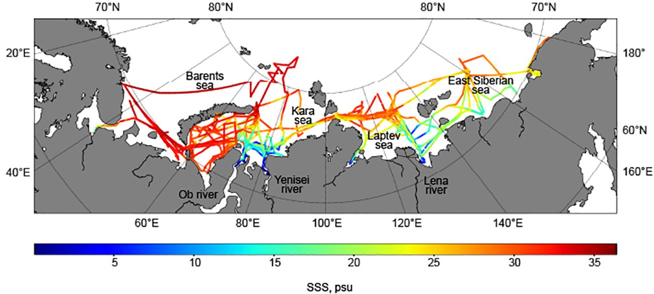
Figure 1 Spatial distribution of in situ salinity data collected in 2015–2021 in the Arctic Ocean and analyzed in this study.

Multiple in situ measurements demonstrated that the Ob-Yenisei and Lena plumes have distinct vertical and lateral salinity gradients at the isohalines of 14–16 psu and at the isohalines of 24–26 psu (Osadchiev et al., 2021a, Osadchiev et al., 2021b). The first frontal zone at 14–16 psu represents transformation of freshwater discharge on synoptic time scales (i.e., several weeks), while the second frontal zone at 24–26 psu represents transformation of freshwater discharge on seasonal time scales (i.e., several months).

The distribution of SSS data values among the analyzed in situ measurements is shown in Figure 2. The majority of the collected data was obtained at areas limitedly affected by river discharge with SSS values exceeding 24 psu. These SSS values will be referred to as “high” salinities. “Low” salinities will refer to values below 15 psu, mainly found in estuarine areas with a strong influence of river runoff. Salinities between 15 and 24 psu will be called “medium” salinities. It should be noted that in (Jang et al., 2021) low salinities (mainly starting from 20 psu) as compared to typical salinities of the World Ocean (33-38 psu) were examined. However, considering the specific characteristics of the Arctic seas, in this study, salinities above 24 psu are referred to as high salinities since the measured SSS values covers wide range of values from 0 to 35 psu.

Figure 2

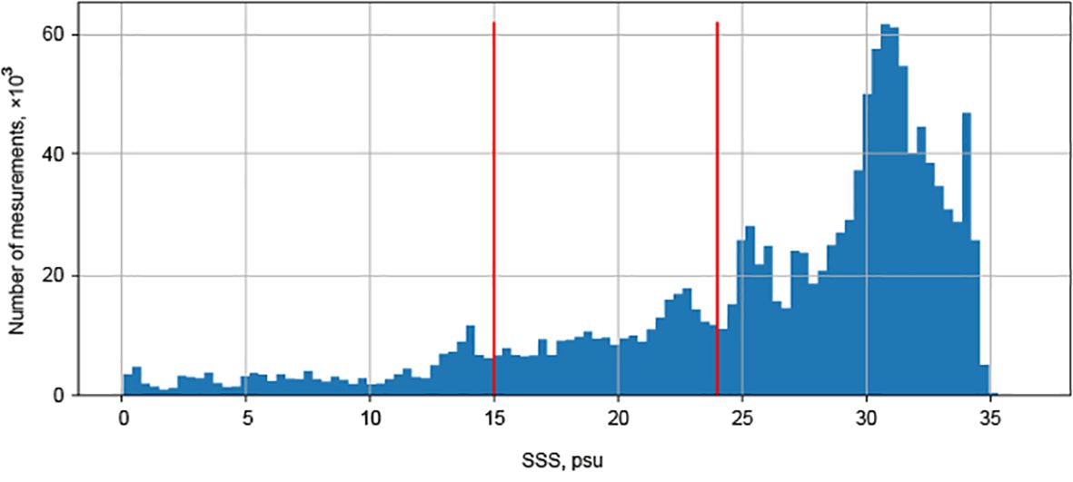
Figure 2 Salinity distribution among the analyzed in situ measurements. Red vertical lines demonstrate thresholds between low (< 15 psu), medium (between 15 and 24 psu) and high (> 24 psu) salinity classes.

3 Methodology

3.1 Data used

In this study, the SMAP SSS is improved using ML approaches. The ML models utilize a feature set consisting of 13 variables, namely, 12 variables are derived from the standard SMAP algorithm and one is the SMAP salinity product obtained through the standard algorithm. These variables were described in Section 2.1. Consideration of these features is motivated by several reasons. First, the complexity of the problem is a key consideration. Improving SSS estimates across the entire range of values from 0 to 35 psu using only brightness temperature data is found to be insufficient (Fore et al., 2016). Second, errors in the salinity retrieval algorithms caused by the proximity to land or sea ice provide significant challenges. Ice drift, formation, and melting could significantly decrease the accuracy of standard algorithms (Fore et al., 2016; Reul et al., 2020; Meissner and Manaster, 2021). To address these challenges, features characterizing the land and sea ice fractions are included to the analyzed data set. Furthermore, the quality of the incoming microwave radiation could be affected by the solar angle at the study area. Features describing the solar angle serve as indicators of data quality for the ML models.

In situ data is used for training and validation of ML models. In situ and satellite measurements are compared according to their spatial and temporal proximity. In situ and satellite data is considered to be from the same grid cell and compared if the distance between the satellite and in situ measurement points does not exceed 10 km, and the time difference between measurements is no more than 3 hours. In different studies, the time difference for comparison ranges from up to 12 hours (Boutin et al., 2018) to up to 3 hours (Jang et al., 2021). In this study, the small acceptable time difference can be attributed to the high temporal variability in surface salinity due to the energetic dynamics of river plumes. The data is split into training and testing sets for model validation based on day of year, meaning all data collected within a single calendar day is included either to the training or testing set. The verification dates are randomly selected from the entire data set, ensuring that the feature descriptions and target distributions of variables in the testing set align with those in the training data.

During the matching process, for each satellite measurement point, all in situ measurements that meet the mentioned spatial and temporal criteria are selected. As a result, there can be multiple in situ measurements corresponding to one satellite measurement and vice versa, introducing natural variability into the data. In total, after the matching, there are approximately 500,000 pairs of satellite–in situ measurements, with around 350,000 pairs representing different in situ measurement points. On average, each in situ measurement corresponds to 1.4 different sets of satellite features.

To retrieve atmospheric pressure, temperature, and near-surface wind fields in the vicinity of in situ measurements, some ML models consider two-dimensional ERA-5 data in addition to SMAP data as a part of the feature description (Hersbach et al., 2020). ERA-5 data is distributed on a regular grid with a spatial resolution of 0.25° and a temporal resolution of 1 hour. In situ and satellite measurements are transferred to this grid for correct matching with ERA-5 data.

Processing of ERA-5 data aims to improve the accuracy of retrieving of atmospheric conditions around the observation points. These fields are considered in an approximate neighborhood of 250 km in both the meridional and zonal directions, which corresponds to 2.25° in the meridional direction and 8° in the zonal direction from the observation point.

3.2 Comparison of in situ and satellite SSS data

As discussed in (Boutin et al., 2016; Reul et al., 2020), several issues arise when validating satellite algorithms for retrieving SSS using in situ data. The first issue is that in situ measurements are pointwise samples, and their density is usually much higher than that of satellite data. Satellite data, on the contrary, is spatially averaged data, with resolution starting from several kilometers. Additionally, the variables used in the standard SMAP algorithm are taken from various sources and then transferred to a unified spatial and temporal grid. This interpolation may also lead to additional biases.

The second issue of matching satellite and in situ data is that satellite radiometers operating in the L-band range receive signals from the upper millimeters of the ocean surface. In situ measurements are typically taken at depths of 2–4 meters. In case of high stratification in the upper layer, which can be caused by high precipitation and strong evaporation (however, not typical for the Arctic Ocean during the warm season (Haine et al., 2015)), as well as the inflow of river discharge and ice melting (both processes play a significant role in the study region), in situ measurements may not correspond to the satellite measurements due to the difference in measurement depth, even if they were conducted with low spatial and temporal difference (Boutin et al., 2016).

To examine the influence of vertical stratification in the upper layer of Arctic shelf areas, this study considers in situ measurements conducted in 2018–2021. The aim of this consideration is to verify that at the depth of in situ measurements (2–4 meters), salinity differs from satellite-derived SSS less than a certain threshold value. This value was chosen equal to 1 psu, and the difference between salinity at 5 meters depth and the upper measured salinity in the same profile was examined. Note that measurements of sea salinity exactly at the sea surface generally are not available due to the physical size of CTD instruments, presence of sea surface waves, air entrapment during probe submersion and other factors. In fact, the upper reliable measurement is obtained at a the depths of 1.5–2.5 meters, and this value was compared with the salinity measured at 5 meters in this study. It is assumed that the water from the surface to a depth of 2 meters is mixed by wind waves (Rainville et al., 2011), and the described comparison accurately solves the problem of relation between the satellite and in situ measurements (Boutin et al., 2016).

The map of vertical measurements at hydrographic stations in the Arctic Ocean is shown in Figure 3. Blue points represent stations, where the difference between the upper measured salinity value and the value at the depth of 5 meters is less than 1 psu, red points represent stations where the difference is greater than 1 psu.

Figure 3

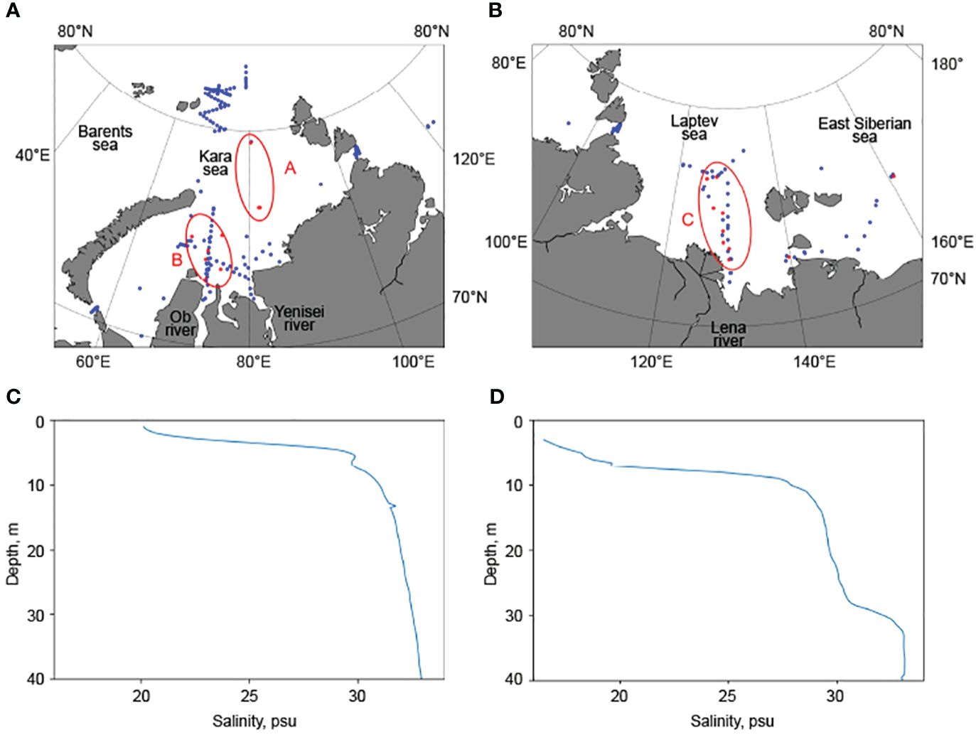
Figure 3 Location of stations with small (< 1 psu, blue dots) and large (> 1 psu, red dots) salinity difference between the surface layer and the depth of 5 m in the Kara Sea (A) and in the Laptev and East Siberian seas (B). Examples of vertical salinity profiles with large salinity difference between the surface layer and the depth of 5 m due to intense sea ice melting (C) and within river plumes (D).

Out of nearly 300 profiles demonstrated in Figure 3, in 93% of cases difference between surface salinity and salinity at the depth of 5 meters is < 1 psu. Figures 3C, D show typical profiles at stations that do not satisfy this condition. For instance, measurements at stations of group A were conducted during intense sea ice melting in close proximity to the measurement point (Figure 3C). Melting of sea ice reduces salinity of surface layer in the Arctic Ocean, because sea ice salinities (< 10 psu) are much less that seawater salinities (Cox and Weeks, 1974; Tucker et al., 1987; Wang et al., 2020). Melting of sea ice releases large freshwater volume to the surface sea layer reducing its salinity till the depths of 5-10 m (Perovich et al., 2021). Salinity at greater depths remains stable, which is demonstrated in Figure 3C.

Stations in groups B and C were conducted within the Ob-Yenisei and Lena river plumes, respectively (Figure 3D). The stratification in the near-surface layer here is not as strong as in the case of intense sea ice melting, but it exceeds the considered threshold value by 1 psu.

However, the overwhelming majority of profiles exhibit small difference between salinity at the depth of 5 meters and at the sea surface indicating that the methodology of comparing satellite data and in situ measurements is correct.

3.3 Machine learning approaches

3.3.1 Classical ML models

Machine learning (ML) approaches were previously used for processing remote sensing data, including SSS retrieval (Chen and Hu, 2017; Pham et al., 2017; Wang and Deng, 2018; Bao et al., 2019; Cho et al., 2020; Kim et al., 2020; Jang et al., 2021). This study considers ML models from classical methods like Random Forest (RF) and Gradient Boosting (GB) to deep artificial neural networks (ANN) of various architectures. A linear regression (LR) model is used as a baseline model to assess the quality of the results that can be obtained using ML models.

Certainly, in this study an improvement in the accuracy of SSS estimation compared to standard satellite algorithms is expected, and models that do not achieve such results are not considered meaningful. At the same time, we use a simple linear model for comparing the quality of results obtained by different models.

The first of the main ML models considered in the study is the RF model (Breiman, 2001), which is often used for regression and classification tasks. This model is an ensemble of decision trees, each of them individually may provide low quality in solving the task, but by having a large number of them, a better performance could be achieved. Each decision tree consists of nodes that split the input features and leaves those, which contain the value of the target function. The ensemble consists of multiple trees with different and random parameters. In this study, a model implemented in the scikit-learn library (Pedregosa et al., 2011) is used.

The second classical ML model considered in the study is GB. Similarly as if was in RF, this model is also based on weaker models. However, unlike RF, where decision trees are built independently for each sample, in GB this process happens sequentially, and earlier trees are used to improve the subsequent ones. The main variable hyperparameter of GB model is the maximum number of constructed trees. CatBoost Gradient Boosting model implemented by Yandex (Dorogush et al., 2018) is used in this study. The search for optimal hyperparameters for the RF and GB models is performed using the optuna framework (Akiba et al., 2019).

All three described classical models are considered in two configurations: “single-level” and “two-level”. In the “single-level” configuration, the models are used to directly predict the SSS values over the entire range of measured natural values, effectively solving the regression task (Figure 2). The “two-level” configuration has a more complex configuration. First, it solves a classification problem to split the salinity values into “low”, “medium”, and “high” as described in Section 2.3. Then, based on the predicted class, a regression model is applied to predict SSS.

The complexity of the “two-level” configuration is driven by highly uneven distribution of in situ SSS. The majority of the measurements refer to high salinity class, which means that these data would be encountered more frequently during the model training. It means that the model would be well-trained on the part of the data spectrum where the density of the distribution is high, but would perform noticeably worse on the opposite side of the salinity spectrum. To account this issue, methods of non-uniform data sampling grouped by a certain feature, such as the target variable value, are commonly applied. In this study, instead of adjusting the weight coefficients for individual data points, different models are trained on separate classes. This approach is considered more preferable, because the determined classes mainly correspond to fundamentally different water masses. If waters with high salinity values have pure oceanic origin, the low salinity values indicate the formation of these waters as a result of mixing of river runoff with saline seawater.

3.3.2 Artificial neural networks

Apart from the classical models, various types of artificial neural networks (ANN) are also examined in this study. One such type is the Multilayer Perceptron (MLP), which is the most common architecture of ANN. It comprises multiple neurons interconnected to map the input features to the target variable. In this study, the model involves a feature set consisting of 13 satellite variables.

Similarly to the classical models, the neural network approach also considers a “two-level” analog. However, unlike the classical solutions where the classification and regression tasks were solved sequentially, in this algorithm, the class values obtained from the satellite variables themselves serve as input features for the SSS retrieval. The architecture of this model is demonstrated in Figure 4A.

Figure 4

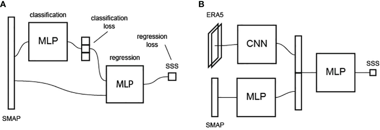
Figure 4 Neural network models applied in this study including composite classification and regression model (A) and composite model considering SMAP and ERA-5 features (B).

The last configuration of artificial neural networks considered in this study allows inclusion of two-dimensional fields of atmospheric pressure, temperature, wind speed and wind direction in addition to satellite measurements near the observation point. The architecture of this model is depicted in Figure 4B.

To extract features from the two-dimensional data, Convolutional Neural Networks (CNN) are employed. To enhance generalization and efficiently extract meaningful features, the convolutional part of the overall neural network is pre-trained using an autoencoder approach on data from July to October of the years 2000–2019. Data for pre-training is randomly selected uniformly across time and space. The encoder for the two-dimensional data has an AlexNet-like neural network model configuration (Krizhevsky et al., 2012), which consists of convolutional layers with gradually decreasing dimensions and increasing numbers of channels. At each convolutional stage, two additional channels representing the two-dimensional coordinates of the considered data fields are added to the input features. This approach aids in enhancing the overall informativeness of the extracted features.

Another type for the encoder is based on a ResNet-like neural network model configuration (He et al., 2016). This model consists of blocks that include two convolutional layers, optional dimension reduction and/or channel increase, as well as feature transport from the block input and its sum with the block output. In this study, the convolutional layer is also enhanced with spatial positional encoding. In all neural network models used, a nonlinear activation function Mish (Misra, 2019) is added between each pair of weight layers, which has a number of advantages over the classical Relu activation function (Nair and Hinton, 2010).

Pre-trained convolutional encoder derives features from two-dimensional physical field description and adds them to the satellite feature set, processed through MLP. From all the obtained variables, a unified vector is formed and fed into the final MLP, which retrieves SSS. The architecture of the entire model is demonstrated in Figure 4B.

For training of all models used in this study, the mean squared error (MSE) between the model predicted values and the measured SSS values is used as the loss function. In addition, the correlation coefficient r is considered as a quality metric. Optimization of the models is not based on this metric during training, but it is taken into account when interpreting the obtained results.

4 Results and discussion

4.1 Accuracy of SMAP SSS data in the study area

To examine the quality of standard SMAP SSS algorithm in the Arctic shelf areas, the differences between the measured in situ SSS values and the satellite estimates were calculated. Figure 5 demonstrates the distribution of errors in satellite salinity relative to the measured values. The Root Mean Squared Error (RMSE) is 3.15 psu, and the correlation coefficient r between them is 0.82. In addition to the entire error distribution, errors for the low, medium, and high SSS value classes (as defined in Section 2.3) are considered. Such error distributions are presented in Figures 5C–E.

Figure 5

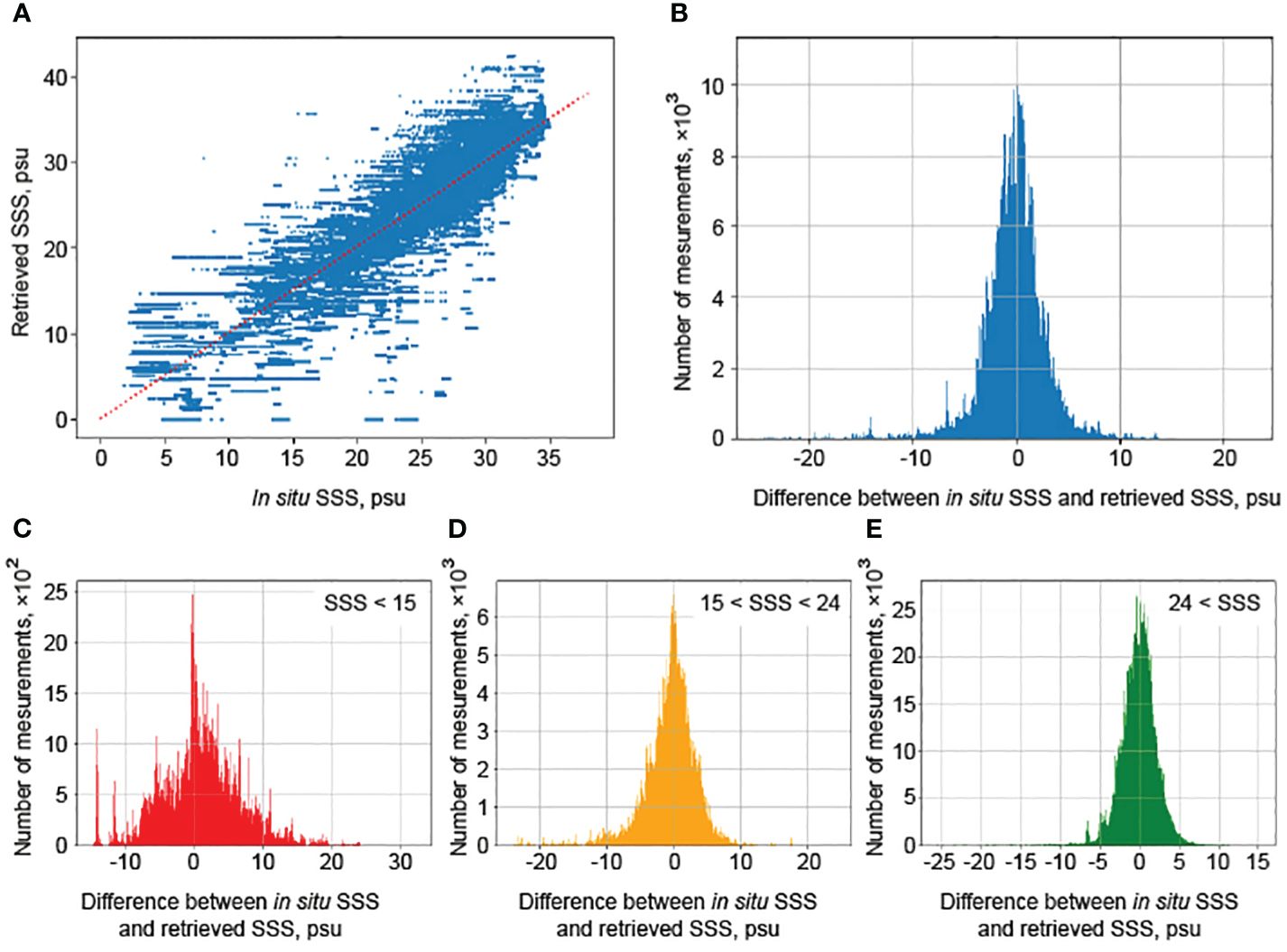
Figure 5 Characteristics of SMAP sea surface salinity retrieval algorithm assessed using in situ salinity measurements in Arctic Ocean: a scatter diagram of SMAP SSS compared to in situ salinity (A), error distributions for the full range of salinity (B), and for low (C), medium (D) and high (E) salinity values.

For the described in Section 2.3 classes, the RMSE values are 6.06 psu, 3.41 psu, and 2.41 psu, respectively. Satellite algorithms perform best on high SSS values, i.e., outside the zone of significant influence of river runoff. The salinity of these waters is the closest to the typical values in the World Ocean, hence, the best performance of standard satellite algorithms is achieved on this SSS class. At the same time, the majority of the measured SSS values belong to this class, and therefore the quality of both algorithms, standard and developed in this study, is mainly determined by their performance on this salinity class. It should also be noted that the standard algorithm predicts SSS values above 40 psu at some observation points. However, values above 35 psu are not observed in the considered set of in situ data.

Since a significant part of the Arctic Ocean is characterized by low SSS values, the aim of this study is to develop a model capable of accurately estimating SSS at the entire range of SSS values including low salinities. While errors of the satellite algorithms relative to the measured values follow normal distribution for high and medium salinity values, the error distribution for low salinity values appears to be more complex. Although the mean error of standard satellite algorithms here is 6.06 psu, individual differences are up to 30 psu. Therefore, it is necessary to consider the loss function and quality metrics for all major parts of the target variable distribution.

As previously was noted in (Fore et al., 2016; Qin et al., 2020; Reul et al., 2020), the performance of satellite algorithms is influenced by various different conditions at the observation point, such as atmospheric temperature and pressure, the presence or absence of coastline or sea ice, etc. We investigated the dependency of error of standard algorithms relative to observations at different months of year. Despite an overall RMSE of 3.15 psu, the highest error occurs in July, reaching 4.16 psu. This feature is caused by the fact that nearly half of in situ measurements in this month were located in coastal areas with low SSS values. Satellite algorithms perform best in August and September, with RMSE values of 2.72 psu and 2.98 psu, respectively. Almost half of all measurements were performed within these two months, and the determined accuracy can be considered as mostly correct. The largest number of measurements is collected in October, with a significant part of them referring to medium SSS values. The RMSE value for October is 3.33 psu. Decrease in accuracy with a relatively low presence of freshwater can be explained by low sea surface temperatures in October (Osadchiev et al., 2023a), which reduce the sensitivity of satellite radiometers to the incoming microwave radiation (Kolodziejczyk et al., 2016; Dinnat et al., 2019; Reul et al., 2020). Another reason is the increase of ice coverage in October, which reduces the performance of standard SSS retrieval algorithms.

4.2 Application of different models

The most classical neural network ML models showed an improvement in the quality of SSS retrieval compared to standard algorithms. The results are presented in Table 1. In this study, linear regression is considered as the baseline ML model. Some linear models have already been constructed to correct errors in satellite algorithms (Kolodziejczyk et al., 2016; Qin et al., 2020). Currently, the linear model is not used as the main method for SSS retrieval, but it can be utilized as an estimation of possible ML performance. So, the linear regression model overall showed higher results as compared to standard algorithms (Table 1), and the performance of the other models can be compared to the performance of the linear model.

Table 1

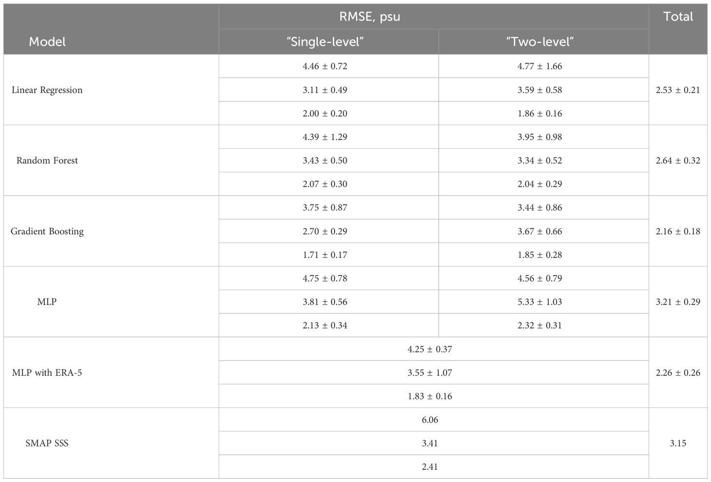
Table 1 The results of the applied ML models for retrieving SSS. For each model MSE for low, medium and high SSS values are demonstrated.

The two main classical ML models considered in this study are RF and GB. As described in Section refmodels, these models were examined in both a “single-level” and “two-level” approach. The hyperparameters of the models were tuned using the optuna framework.

RF and GB models yield improved quality compared to the standard satellite algorithms. However, the RF model demonstrates inferior SSS retrieval results compared to the linear model. On the contrary, the quality of GB model surpasses both the LR and RF models. Besides, “single-level” models, which were trained on the entire spectrum of SSS values, perform better on high and medium SSS values.

Neural network models trained on satellite vector feature set did not show an improvement in SSS quality compared to standard algorithms. Moreover, they yielded poor results while retrieving medium SSS values, performing worse than the standard algorithms. The error values presented in Table 1 for these models are significantly higher as compared to the classical models.

The addition of two-dimensional atmospheric data from ERA-5 also did not improve the results despite high performance of pre-trained encoder model for climate data extraction.

4.3 Selection of the best model

As a result of applying classical ML models, the best results were achieved using GB model, both for the described SSS classes and for the entire distribution. RMSE values for the difference between in situ SSS values with predicted ones (Table 1), improved as compared to the results of the standard SMAP algorithm. The correlation coefficient increased from 0.82 to 0.90. The characteristic distributions of SSS error obtained using the best algorithms are shown in Figure 6.

Figure 6

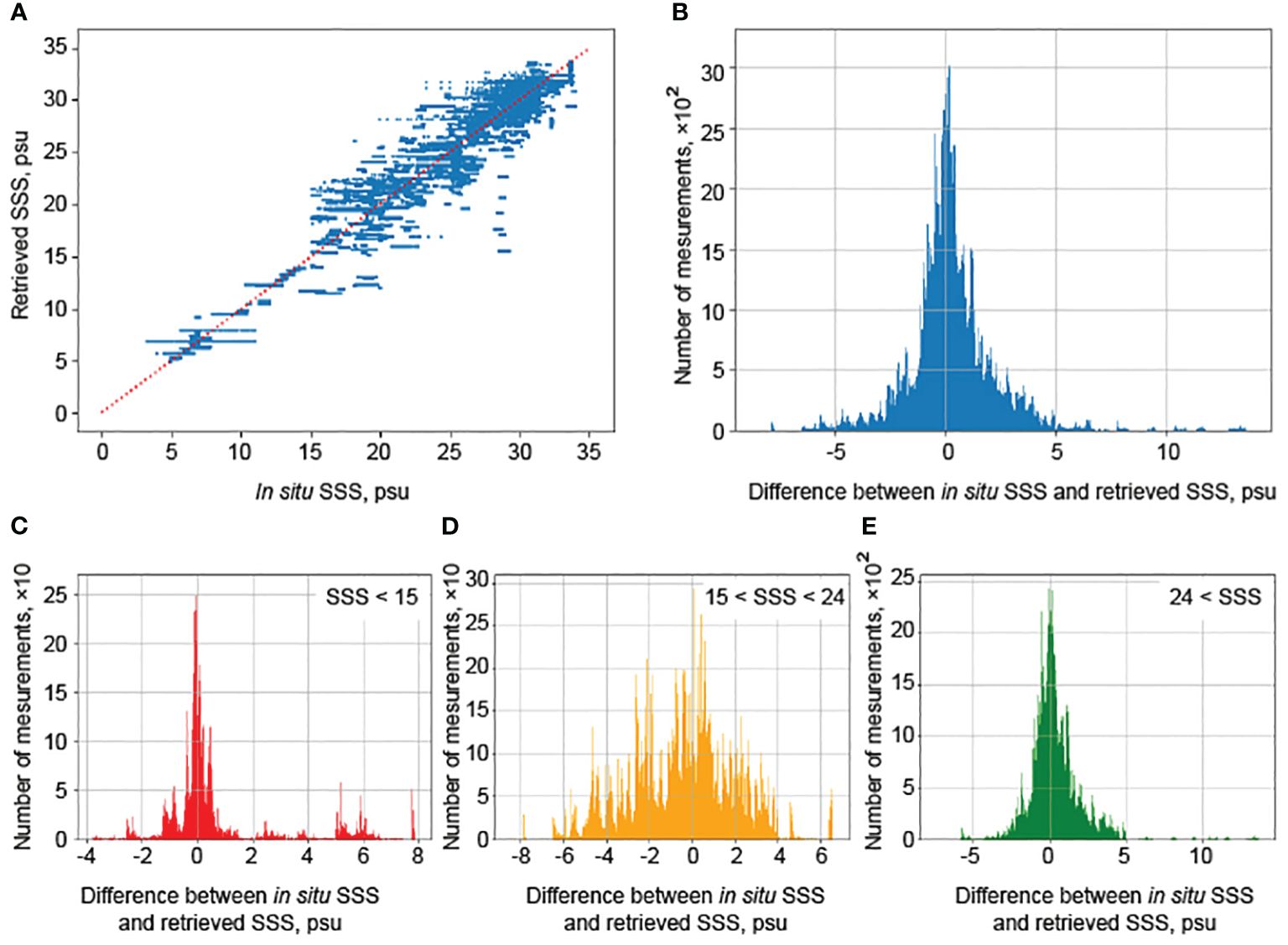
Figure 6 Characteristics of a model providing the best SSS approximation quality: a scatter diagram of predicted SSS compared to in situ salinity (A), error distributions for the full range of salinity (B), and for low (C), medium (D) and high (E) salinity values.

The best ML model improved quality of the standard algorithms. The overall error for all dataset was 2.15 ± 0.18 psu (for the standard algorithm it was 3.15 psu). For the selected low, medium, and high SSS classes, the errors were 3.43 ± 0.86, 2.70 ± 0.29, and 1.71 ± 0.17 psu, respectively (for the standard algorithm, they were 6.06, 3.41, and 2.41 psu, respectively). The best quality, for both the standard algorithm and the models constructed in this study, is achieved for high SSS values. The worst results of the models are observed for low SSS values. This feature is caused by relatively small amount of data in this range, as well as complex spatial and temporal variability of river plumes.

Note that there are different x- and y-axis in Figures 5, 6, because Figure 5 demonstrates the whole set of data, while Figure 6 demonstrates only the test set. Also, Figures 5, 6 show different orders of errors between the satellite algorithms and the developed model. The errors in the satellite algorithms exceed 20 psu, and we choose a wider x-axises in panels (B)–(E) in Figure 5 than those in Figure 6.

Further analysis of the obtained results will be conducted using the best constructed “two-level” composite model. It consists of a classifier, based on the results of which the SSS value is predicted according to the algorithm for low SSS if the low salinity class was predicted, or according to the algorithm trained on the entire range of SSS values if the predicted class differs from the low salinity class.

4.4 Model error distribution

As was mentioned earlier, the performance of satellite algorithms depends on the geographical location and atmospheric conditions of the study area. Some features considered in the SSS retrieval model aim to account for factors such as proximity of the observation point to the coastline or to sea ice, which can negatively impact the quality of standard algorithms (Fore et al., 2016; Kao et al., 2018; Olmedo et al., 2018; Qin et al., 2020; Reul et al., 2020).

To assess the quality of the constructed model, the spatial distribution of errors is examined on the test data set (Figure 7A). It should be noted that the summer measurements mainly correspond to the Kara Sea and do not cover other regions, as those areas are mainly ice-covered during this period (Osadchiev et al., 2021b). Errors in these regions occur mainly near the coastline and in the ice melting areas, as well as in the regions influenced by river runoff. Errors decrease at the observation points located off these areas and are close to zero in the open sea.

Figure 7

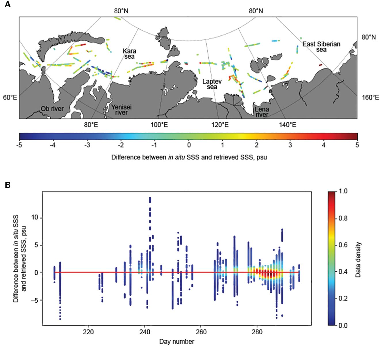
Figure 7 Spatial (A) and temporal (B) error distribution of SSS.

A similar pattern also takes place during the autumn period. The model tends to underestimate the SSS values at the boundaries of river plumes and tends to overestimate them closer to the estuarine zones. In ice formation areas, SSS values also become underestimated. Errors occurring near the ice edge can be explained by the fact that the water surface near ice masses is intensively freshened due to sea ice melting (Zhang et al., 2023). At the same time, the salinity of seawater sharply increases at the depth of several meters. Since satellite measurements correspond to the upper millimeters of the ocean surface (Reul et al., 2020), and the in situ data used to verify the algorithms are taken at depths of 2–4 meters, greater discrepancies between algorithm products and in situ SSS values may be observed in such areas, as discussed in section 3.2. The use of sea ice fraction as a feature in the ML model aims to account for this bias, but it is not possible to adequately correct the errors in such areas.

Figure 7B demonstrates dependence of the difference between in situ and predicted SSS values obtained from the constructed algorithm, with the density of data points plotted by the day of the year. First, the majority of the data points were collected in September and October, which corresponds to the period with the highest number of in situ SSS measurements. Secondly, the difference distribution is concentrated around zero, and the amplitude of this difference remains roughly constant over time. This indicates that the constructed model is able to accurately estimate SSS values during both summer and autumn periods, even when sea surface temperature decreases.

4.5 “Two-level” models

Overall, based on the results of all constructed models (Table 1), it can be concluded that “single-level” models perform better for high and medium salinity values, while “two-level” models show higher quality for low values. This can be explained, first, by the distribution of the in situ data, i.e., the distribution of the target variable (Figure 2). It has almost normal distribution with a clearly pronounced peak around 29 psu and a long tail towards low salinity values. As was expected, the model performance decreases as the target variable values move away from the peak, resulting in the worst resolution in the low salinity range. This problem could not be resolved by common normalization of the entire distribution, because the amount of data related to the high salinity class accounts for approximately 70% of the total number of available measurements. Once the data would be normalized, the distribution peak would not shift significantly, and its structure would remain almost unchanged.

Second, the low quality for low and medium salinity values in the “two-level” models may be related to relatively poor classification accuracy. In the best models, the accuracy metric reaches a value of 0.90 ± 0.02. However, it is important to understand that this relatively high indicator is mainly determined by the large amount of data in the high salinity class, which is easily classified. The F₁ score provides a better insight into the problem, for low salinity values, it is 0.70 ± 0.13, for medium values it is 0.75 ± 0.05, and for high values it is 0.96 ± 0.01. The low quality for the first two classes can be explained by arbitrary division into medium and high values, because the threshold value equal to 15 psu is not observed at the distribution structure.

Since the best quality was achieved by the “two-level” composite model, which has relatively poor classification accuracy, it is important to consider the quality of the algorithms not only on the defined salinity classes but also at the boundary between the low and medium classes. The objects that were misclassified and were processed by the “wrong” algorithm when solving the regression task are of special interest. Classification errors occur in two main cases. First, such data are geographically located in areas where freshwater masses prevail. This is observed from the second half of August to mid-September. Second, classification errors could occur in late October during the beginning of the ice formation period, and at that time, they might be outside the influence of river plumes.

SSS values for objects belonging to low salinity class, i.e., up to 15 psu, but classified as medium salinity values, are predicted by “one-level” algorithm. In this case, SSS is retrieved with relatively high accuracy. This is because during the training of “one-level” models, there were low salinity values in the training data set, and the model operates them well. Another situation occurs when objects with initially medium salinity values are classified as having low salinity values. With such data, the model trained on low salinity class performs significantly worse, assigning them low salinity values. Thus, summarizing the fact that in the first case, the salinity values are determined well, and in the second case, the model tends to underestimate the real values, it could be concluded that in general, around 15 psu, the predicted SSS values are slightly underestimated compared to the in situ ones. This is also demonstrated by the quantile-quantile plot shown in Figure 8A. In addition, SSS values around 25 psu are also underestimated. This can be explained by the fact that the inner plume front bounding the estuarine zone correspond to 15 psu, and the outer boundary of the plume correspond to 25–28 psu. In these areas, there is active mixing of different water masses, and the quality of SSS retrieval algorithms decreases.

Figure 8

Figure 8 Quantile-quantile plot for in situ and predicted SSS (A). Error distribution for low salinity values, predicted by “single-level” model (B).

However, despite all the flaws of “two-level” models, a regression model trained on the low salinity class and working only on it shows significantly higher quality than the “one-level” model on this class. Although the error values of the constructed algorithms seem to be close (3.43 ± 0.86 for the “two-level” model and 3.75 ± 0.87 for the “one-level” model), a significant difference is observed in the characteristic distribution of the error. In the first case, it has the nature of a normal distribution with a pronounced peak at zero, while when using a single model, the error distribution has several peaks, its center does is not located at zero, and the model tends to predict overestimated SSS values (Figure 8B).

Since classification is important for obtaining results on low salinity values, but at the same time its quality does not allow to achieve expected results, another model architecture was considered, which has been developed in neural network approaches. Classification is performed, but the obtained class is used as a feature along with the original satellite features. However, this approach did not yield the expected results when using classical methods. The quality of the final result did not improve for low salinity values.

4.6 Feature importance

Feature importance for the best model is demonstrated in Figure 9. Note that there are different y-axis in Figures 9A, B. The “single-level” model has an expected feature importance balance: SSS from the standard SMAP algorithm plays the most significant role here, as this variable is correlated with the target variable at 0.82 (Figure 9A). Among other features, the solar zenith angle, sea ice fraction, solar radiation flux, and the brightness temperature in horizontal polarization are highlighted.

Figure 9

Figure 9 Feature importance for the “single-level” model (A) and for low salinity values model (B).

A more complex configuration is observed for low salinity values in the “two-level” model (Figure 9B). In this case, the salinity value from the standard algorithm does not play a decisive role, which can be explained by the relatively low accuracy of the standard algorithms for this part of the SSS distribution. In addition to features describing the position of the Sun above the observation point and the land and ice fractions, the solar radiation flux, determined by cloud cover, plays an important role, similar to the previous case. Solar energy has a significant influence on the signal emitted from the water surface (Meissner et al., 2018), which explains the high significance of this feature in the SSS estimation. The role of wind, especially its direction, has increased. It is interesting to note the different significance of the zonal and meridional components. In the considered Arctic seas, the meridional wind usually brings warm air from the continent, while the zonal wind corresponds to the general direction of atmospheric eastward circulation in the region. Finally, the signal from the sea surface, i.e. the brightness temperature in horizontal and vertical polarizations, has a significant influence on the model results. This is the main signal directly obtained from the satellite, whi most of other features are supplied from external sources.

It is worth noting the high importance of wind and sea surface temperature on the quality of sea surface salinity (SSS) retrieval (Dinnat et al., 2019; Reul et al., 2020). Low sea surface temperature in the Arctic Ocean provides a natural sources of errors, because it decreases the sensitivity of the brightness temperature radiometers (Martínez et al., 2021).

4.7 The resulting SSS data

To examine the spatial and temporal variability of the large river plumes in the Arctic Ocean as well as other water masses based on the improved SSS values, daily and weekly average SSS maps are created for the Eurasian part of the Arctic Ocean. SSS values are calculated at nodes of a regular grid with a step of 0.5° in latitude and 0.125° in longitude. With this step, the grid becomes almost square around 75°N, which corresponds to the center of the study region. These maps allow distinguishing large Ob-Yenisei and Lena plumes, analyzing their boundaries and internal structure during the ice-free period of the year.

As an example, Figure 10 shows typical weekly SSS maps constructed from satellite data from July to November 2020. The maps illustrate the distribution of the Ob-Yenisei and Lena plumes during this period. Sharp increases in area can be observed for both the Ob-Yenisei and Lena plumes during their formation in July, which corresponds to the summer flooding season (Osadchiev et al., 2021a, Osadchiev et al., 2021b). The Lena plume has a significantly larger area (2–3 times) in the Laptev Sea and East Siberian Sea compared to the Ob-Yenisei plume in the Kara Sea. In August-September, the areas of both plumes remain stable, but there is synoptic variability in the position of their boundaries. During this time, the salinity of the plumes gradually increases due to the mixing with underlying saltier seawater under conditions of reduced river runoff during the autumn period (Osadchiev et al., 2021a, Osadchiev et al., 2021b). Clear boundaries of the river plumes are visible until mid-October, after which these boundaries begin to dissipate in the second half of October. By early November, the areas covered by the Ob-Yenisei and Lena plumes become ice-covered.

Figure 10

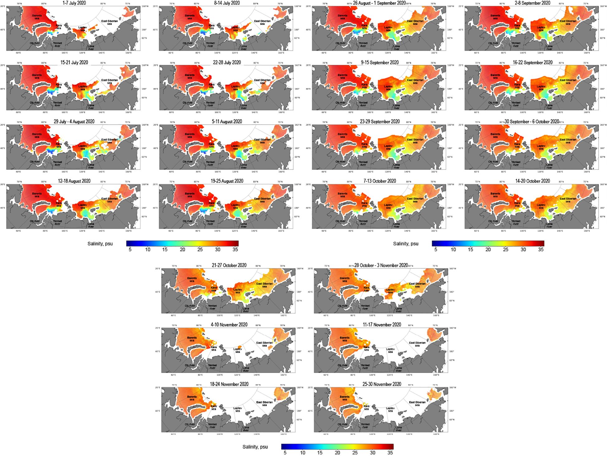
Figure 10 Weekly averaged maps of the reconstructed SSS in the Eurasian Arctic Ocean in July–November 2020.

5 Conclusions

In this study, machine learning approaches are considered to improve satellite salinity in Arctic regions. Vector feature set from SMAP and two-dimensional climatic fields from ERA-5 atmospheric reanalysis are used as feature descriptions. The validation is carried out on in situ data collected during multiple oceanographic expeditions. Almost all the models examined in this study showed an improvement of SSS quality compared to standard algorithms. The best composite model, Gradient Boosting, increased the overall quality of SSS retrieval from 3.15 psu to 2.15 ± 0.18 psu and from 6.06, 3.41, 2.41 to 3.43 ± 0.86, 2.70 ± 0.29, and 1.71 ± 0.17 psu for classes of low, medium, and high salinity values, respectively. Since this model uses only vector satellite features from SMAP, it is possible to retrieve SSS in the Arctic Ocean in near real time.

The constructed model provides high accuracy in investigating the spatial and temporal variability of the major water masses in the surface layer of the Arctic Ocean using surface salinity data. High accuracy of the developed algorithm at low salinity values is especially important for detecting spreading areas of river plumes, where the quality of standard algorithms is low. The constructed SSS maps provide opportunity to quantitatively assess seasonal variability of the boundary and internal structure of the Ob-Yenisei and Lena river plumes during the ice-free period of the year. Further studies, based on the developed algorithm, will be focused on detailed analysis of the seasonal and inter-annual variability of the area and salinity of these river plumes, as well as their dependence on river runoff, wind forcing, and other external forcing factors.

Data availability statement

The original contributions presented in the study are included in the article/supplementary material. Further inquiries can be directed to the corresponding author.

Author contributions

AS: Formal analysis, Investigation, Methodology, Software, Visualization, Writing – original draft, Writing – review & editing. MK: Methodology, Software, Writing – original draft, Writing – review & editing. AO: Conceptualization, Methodology, Writing – original draft, Writing – review & editing.

Funding

The author(s) declare financial support was received for the research, authorship, and/or publication of this article. This research was funded by the Moscow Institute of Physics and Technology Development Program (Priority-2030) (numerical modelling) and the Russian Science Foundation, research project 23-17-00087 (processing of in situ data).

Conflict of interest

The authors declare that the research was conducted in the absence of any commercial or financial relationships that could be construed as a potential conflict of interest.

Publisher’s note

All claims expressed in this article are solely those of the authors and do not necessarily represent those of their affiliated organizations, or those of the publisher, the editors and the reviewers. Any product that may be evaluated in this article, or claim that may be made by its manufacturer, is not guaranteed or endorsed by the publisher.

References

Akiba T., Sano S., Yanase T., Ohta T., Koyama M. (2019). “Optuna: A next-generation hyperparameter optimization framework,” in Proceedings of the 25th ACM SIGKDD international conference on knowledge discovery & data mining. (New York, NY, United States: Association for Computing Machinery) 2623–2631. doi: 10.1145/3292500.3330701

CrossRef Full Text | Google Scholar

Bao S., Zhang R., Wang H., Yan H., Yu Y., Chen J. (2019). Salinity profile estimation in the pacific ocean from satellite surface salinity observations. J. Atmospheric Oceanic Technol. 36, 53–68. doi: 10.1175/JTECH-D-17-0226.1

CrossRef Full Text | Google Scholar

Boutin J., Chao Y., Asher W. E., Delcroix T., Drucker R., Drushka K., et al. (2016). Satellite and in situ salinity: Understanding near-surface stratification and subfootprint variability. Bull. Am. Meteorological Soc. 97, 1391–1407. doi: 10.1175/BAMS-D-15-00032.1

CrossRef Full Text | Google Scholar

Boutin J., Vergely J.-L., Marchand S., d’Amico F., Hasson A., Kolodziejczyk N., et al. (2018). New SMOS sea surface salinity with reduced systematic errors and improved variability. Remote Sens. Environ. 214, 115–134. doi: 10.1016/j.rse.2018.05.022

CrossRef Full Text | Google Scholar

Breiman L. (2001). Random forests. Mach. Learn. 45, 5–32. doi: 10.1023/A:1010933404324

CrossRef Full Text | Google Scholar

Carmack E. C., Yamamoto-Kawai M., Haine T. W., Bacon S., Bluhm B. A., Lique C., et al. (2016). Freshwater and its role in the arctic marine system: Sources, disposition, storage, export, and physical and biogeochemical consequences in the arctic and global oceans. J. Geophysical Research: Biogeosciences 121, 675–717. doi: 10.1002/2015JG003140

CrossRef Full Text | Google Scholar

Chen S., Hu C. (2017). Estimating sea surface salinity in the northern gulf of Mexico from satellite ocean color measurements. Remote Sens. Environ. 201, 115–132. doi: 10.1016/j.rse.2017.09.004

CrossRef Full Text | Google Scholar

Cho D., Yoo C., Im J., Lee Y., Lee J. (2020). Improvement of spatial interpolation accuracy of daily maximum air temperature in urban areas using a stacking ensemble technique. GIScience Remote Sens. 57, 633–649. doi: 10.1080/15481603.2020.1766768

CrossRef Full Text | Google Scholar

Cox G. F., Weeks W. F. (1974). Salinity variations in sea ice. J. Glaciology 13, 109–120. doi: 10.3189/S0022143000023418

CrossRef Full Text | Google Scholar

Dinnat E. P., Le Vine D. M., Boutin J., Meissner T., Lagerloef G. (2019). Remote sensing of sea surface salinity: Comparison of satellite and in situ observations and impact of retrieval parameters. Remote Sens. 11, 750. doi: 10.3390/rs11070750

CrossRef Full Text | Google Scholar

Dorogush A. V., Ershov V., Gulin A. (2018). Gradient boosting with categorical features support. arXiv. doi: 10.48550/arXiv.1810.11363

CrossRef Full Text | Google Scholar

Durack P. J., Lee T., Vinogradova N. T., Stammer D. (2016). Keeping the lights on for global ocean salinity observation. Nat. Climate Change 6, 228–231. doi: 10.1038/nclimate2946

CrossRef Full Text | Google Scholar

Entekhabi D., Njoku E. G., O’neill P. E., Kellogg K. H., Crow W. T., Edelstein W. N., et al. (2010). The soil moisture active passive (SMAP) mission. Proc. IEEE 98, 704–716. doi: 10.1109/JPROC.2010.2043918

CrossRef Full Text | Google Scholar

Fore A. G., Yueh S. H., Tang W., Stiles B. W., Hayashi A. K. (2016). Combined active/passive retrievals of ocean vector wind and sea surface salinity with smap. IEEE Trans. Geosci. Remote Sens. 54, 7396–7404. doi: 10.1109/TGRS.2016.2601486

CrossRef Full Text | Google Scholar

Fournier S., Lee T., Tang W., Steele M., Olmedo E. (2019). Evaluation and intercomparison of smos, aquarius, and smap sea surface salinity products in the arctic ocean. Remote Sens. 11, 3043. doi: 10.3390/rs11243043

CrossRef Full Text | Google Scholar

Garcia-Eidell C., Comiso J. C., Dinnat E., Brucker L. (2017). Satellite observed salinity distributions at high latitudes in the n orthern h emisphere: A comparison of four products. J. Geophysical Research: Oceans 122, 7717–7736. doi: 10.1002/2017JC013184

CrossRef Full Text | Google Scholar

González-Gambau V., Olmedo E., Martínez J., Turiel A., Durán I. (2017). Improvements on calibration and image reconstruction of SMOS for salinity retrievals in coastal regions. IEEE J. Selected Topics Appl. Earth Observations Remote Sens. 10, 3064–3078. doi: 10.1109/JSTARS.4609443

CrossRef Full Text | Google Scholar

Haine T., Curry B., Gerdes R., Hansen E., Karcher M., Lee C., et al. (2015). Arctic freshwater export: Status, mechanisms, and prospects. Global Planetary Change 125, 13–35. doi: 10.1016/j.gloplacha.2014.11.013

CrossRef Full Text | Google Scholar

He K., Zhang X., Ren S., Sun J. (2016). “Deep residual learning for image recognition,” in Proceedings of the IEEE conference on computer vision and pattern recognition. 770–778.

Google Scholar

Hersbach H., Bell B., Berrisford P., Hirahara S., Horányi A., Muñoz-Sabater J., et al. (2020). The ERA5 global reanalysis. Q. J. R. Meteorological Soc. 146, 1999–2049. doi: 10.1002/qj.3803

CrossRef Full Text | Google Scholar

Horner-Devine A. R., Hetland R. D., MacDonald D. G. (2015). Mixing and transport in coastal river plumes. Annu. Rev. Fluid Mechanics 47, 569–594. doi: 10.1146/annurev-fluid-010313-141408

CrossRef Full Text | Google Scholar

Jang E., Kim Y. J., Im J., Park Y.-G. (2021). Improvement of smap sea surface salinity in riverdominated oceans using machine learning approaches. GIScience Remote Sens. 58, 138–160. doi: 10.1080/15481603.2021.1872228

CrossRef Full Text | Google Scholar

Kao H.-Y., Lagerloef G. S., Lee T., Melnichenko O., Meissner T., Hacker P. (2018). Assessment of aquarius sea surface salinity. Remote Sens. 10, 1341. doi: 10.3390/rs10091341

CrossRef Full Text | Google Scholar

Kerr Y. H., Waldteufel P., Wigneron J.-P., Delwart S., Cabot F., Boutin J., et al. (2010). The smos mission: New tool for monitoring key elements ofthe global water cycle. Proc. IEEE 98, 666–687. doi: 10.1109/JPROC.2010.2043032

CrossRef Full Text | Google Scholar

Kim D.-W., Park Y.-J., Jeong J.-Y., Jo Y.-H. (2020). Estimation of hourly sea surface salinity in the east China sea using geostationary ocean color imager measurements. Remote Sens. 12, 755. doi: 10.3390/rs12050755

CrossRef Full Text | Google Scholar

Kolodziejczyk N., Boutin J., Vergely J.-L., Marchand S., Martin N., Reverdin G. (2016). Mitigation of systematic errors in SMOS sea surface salinity. Remote Sens. Environ. 180, 164–177. doi: 10.1016/j.rse.2016.02.061

CrossRef Full Text | Google Scholar

Krizhevsky A., Sutskever I., Hinton G. E. (2012). “Imagenet classification with deep convolutional neural networks,” in Advances in Neural Information Processing Systems, vol. 25 . Eds. Pereira F., Burges C., Bottou L., Weinberger K. (New York, NY, United States: Association for Computing Machinery).

Google Scholar

Kubryakov A., Stanichny S., Zatsepin A. (2016). River plume dynamics in the Kara Sea from altimetry-based lagrangian model, satellite salinity and chlorophyll data. Remote Sens. Environ. 176, 177–187. doi: 10.1016/j.rse.2016.01.020

CrossRef Full Text | Google Scholar

Le Vine D. M. (2019). Rfi and remote sensing of the earth from space. J. Astronomical Instrumentation 8, 1940001. doi: 10.1142/S2251171719400014

CrossRef Full Text | Google Scholar

Le Vine D. M., Dinnat E. P. (2020). The multifrequency future for remote sensing of sea surface salinity from space. Remote Sens. 12, 1381. doi: 10.3390/rs12091381

CrossRef Full Text | Google Scholar

Le Vine D. M., Lagerloef G. S., Colomb F. R., Yueh S. H., Pellerano F. A. (2007). Aquarius: An instrument to monitor sea surface salinity from space. IEEE Trans. Geosci. Remote Sens. 45, 2040–2050. doi: 10.1109/TGRS.2007.898092

CrossRef Full Text | Google Scholar

Liu Q., Weng F., English S. J. (2010). An improved fast microwave water emissivity model. IEEE Trans. Geosci. Remote Sens. 49, 1238–1250. doi: 10.1109/TGRS.2010.2064779

CrossRef Full Text | Google Scholar

Martínez J., Gabarró C., Turiel A., González-Gambau V., Umbert M., Hoareau N., et al. (2021). Improved BEC SMOS Arctic Sea surface salinity product v3. 1. Earth System Sci. Data Discussions 2021, 1–28. doi: 10.5194/essd-14-307-2022

CrossRef Full Text | Google Scholar

Matsuoka A., Babin M., Devred E. C. (2016). A new algorithm for discriminating water sources from space: A case study for the southern beaufort sea using modis ocean color and smos salinity data. Remote Sens. Environ. 184, 124–138. doi: 10.1016/j.rse.2016.05.006

CrossRef Full Text | Google Scholar

Meissner T., Manaster A. (2021). Smap salinity retrievals near the sea-ice edge using multi-channel amsr2 brightness temperatures. Remote Sens. 13, 5120. doi: 10.3390/rs13245120

CrossRef Full Text | Google Scholar

Meissner T., Wentz F. J., Le Vine D. M. (2018). The salinity retrieval algorithms for the nasa aquarius version 5 and smap version 3 releases. Remote Sens. 10, 1121. doi: 10.3390/rs10071121

CrossRef Full Text | Google Scholar

Meissner T., Wentz F. J., Manaster A., Lindsley R., Brewer M., Densberger M. (2022). Remote sensing systems smap ocean surface salinities [level 2c, level 3 running 8- day, level 3 monthly], version 5.0 validated release (Santa Rosa, CA, USA: Remote Sensing Systems). Available at: www.remss.com/missions/smap. doi: 10.5067/SMP50-2SOCS

CrossRef Full Text | Google Scholar

Misra D. (2019). Mish: A self regularized non-monotonic activation function. arXiv. doi: 10.48550/arXiv.1908.08681

CrossRef Full Text | Google Scholar

Nair V., Hinton G. E. (2010). Rectified linear units improve restricted boltzmann machines. In. Proceedings of the 27th International Conference on Machine Learning (ICML10), June 21-24, 2010, Haifa, Israel.

Google Scholar

Olmedo E., Taupier-Letage I., Turiel A., Alvera-Azcárate A. (2018). Improving SMOS sea surface salinity in the western mediterranean sea through multivariate and multifractal analysis. Remote Sens. 10, 485. doi: 10.3390/rs10030485

CrossRef Full Text | Google Scholar

Osadchiev A., Frey D., Shchuka S., Tilinina N., Morozov E., Zavialov P. (2021a). Structure of the freshened surface layer in the kara sea during ice-free periods. J. Geophysical Research: Oceans 126, e2020JC016486. doi: 10.1029/2020JC016486

CrossRef Full Text | Google Scholar

Osadchiev A., Frey D., Spivak E., Shchuka S., Tilinina N., Semiletov I. (2021b). Structure and inter-annual variability of the freshened surface layer in the laptev and east-siberian seas during ice-free periods. Front. Mar. Sci. 8. doi: 10.3389/fmars.2021.735011

CrossRef Full Text | Google Scholar

Osadchiev A., Medvedev I., Shchuka S., Kulikov E., Spivak E., Pisareva M., et al. (2020a). Influence of estuarine tidal mixing on structure and spatial scales of large river plumes. Ocean Sci. 16, 1–18. doi: 10.5194/os-16-781-2020

CrossRef Full Text | Google Scholar

Osadchiev A., Pisareva M., Spivak E., Shchuka S., Semiletov I. (2020b). Freshwater transport between the kara, laptev, and east-siberian seas. Sci. Rep. 10, 13041. doi: 10.1038/s41598-020-70096-w

PubMed Abstract | CrossRef Full Text | Google Scholar

Osadchiev A., Sedakov R., Frey D., Gordey A., Rogozhin V., Zabudkina Z., et al. (2023a). Intense zonal freshwater transport in the eurasian arctic during ice-covered season revealed by in situ measurements. Sci. Rep. 13, 16508. doi: 10.1038/s41598-023-43524-w

PubMed Abstract | CrossRef Full Text | Google Scholar

Osadchiev A., Viting K., Frey D., Demeshko D., Dzhamalova A., Nurlibaeva A., et al. (2022). Structure and circulation of atlantic water masses in the St. Anna trough in the kara sea. Front. Mar. Sci. 9. doi: 10.3389/fmars.2022.915674

PubMed Abstract | CrossRef Full Text | Google Scholar

Osadchiev A., Zabudkina Z., Rogozhin V., Frey D., Gordey A., Spivak E., et al. (2023b). Structure of the ob-yenisei plume in the kara sea shortly before autumn ice formation. Front. Mar. Sci. 10. doi: 10.3389/fmars.2023.1129331

CrossRef Full Text | Google Scholar

Pedregosa F., Varoquaux G., Gramfort A., Michel V., Thirion B., Grisel O., et al. (2011). Scikit-learn: machine learning in python. J. Mach. Learn. Res. 12, 2825–2830.

Google Scholar

Perovich D., Smith M., Light B., Webster M. (2021). Meltwater sources and sinks for multiyear arctic sea ice in summer. Cryosphere 15, 4517–4525. doi: 10.5194/tc-15-4517-2021

CrossRef Full Text | Google Scholar

Pham T. D., Yoshino K., Bui D. T. (2017). Biomass estimation of sonneratia caseolaris (l.) engler at a coastal area of hai phong city (Vietnam) using alos-2 palsar imagery and gis-based multi-layer perceptron neural networks. GIScience Remote Sens. 54, 329–353. doi: 10.1080/15481603.2016.1269869

CrossRef Full Text | Google Scholar

Qin S., Wang H., Zhu J., Wan L., Zhang Y., Wang H. (2020). Validation and correction of sea surface salinity retrieval from smap. Acta Oceanologica Sin. 39, 148–158. doi: 10.1007/s13131-020-1533-0

CrossRef Full Text | Google Scholar

Rainville L., Lee C. M., Woodgate R. A. (2011). Impact of wind-driven mixing in the arctic ocean. Oceanography 24, 136–145. doi: 10.5670/oceanog

CrossRef Full Text | Google Scholar

Reul N., Grodsky S., Arias M., Boutin J., Catany R., Chapron B., et al. (2020). Sea surface salinity estimates from spaceborne l-band radiometers: An overview of the first decade of observation, (2010–2019). Remote Sens. Environ. 242, 111769. doi: 10.1016/j.rse.2020.111769

CrossRef Full Text | Google Scholar

Supply A., Boutin J., Vergely J.-L., Kolodziejczyk N., Reverdin G., Reul N., et al. (2020). New insights into SMOS sea surface salinity retrievals in the arctic ocean. Remote Sens. Environ. 249, 112027. doi: 10.1016/j.rse.2020.112027

CrossRef Full Text | Google Scholar

Tang W., Yueh S., Yang D., Fore A., Hayashi A., Lee T., et al. (2018). The potential and challenges of using soil moisture active passive (SMAP) sea surface salinity to monitor arctic ocean freshwater changes. Remote Sens. 10, 869. doi: 10.3390/rs10060869

CrossRef Full Text | Google Scholar

Tucker W. B. III, Gow A. J., Weeks W. F. (1987). Physical properties of summer sea ice in the fram strait. J. Geophysical Research: Oceans 92, 6787–6803. doi: 10.1029/JC092iC07p06787

CrossRef Full Text | Google Scholar

Wang J., Deng Z. (2018). Development of a MODIS data based algorithm for retrieving nearshore sea surface salinity along the northern Gulf of Mexico coast. Int. J. Remote Sens. 39, 3497–3511. doi: 10.1080/01431161.2018.1445880

CrossRef Full Text | Google Scholar

Wang Q., Lu P., Leppäranta M., Cheng B., Zhang G., Li Z. (2020). Physical properties of summer sea ice in the pacific sector of the arctic during 2008–2018. J. Geophysical Research: Oceans 125, e2020JC016371. doi: 10.1029/2020JC016371

CrossRef Full Text | Google Scholar

Zabolotskikh E., Chapron B. (2020). Sea surface salinity estimation using AMSR2 measurements over warm oceans. Sea 17, 207–220. doi: 10.21046/2070-7401-2020-17-4-207-220

CrossRef Full Text | Google Scholar

Zhang H., Bai X., Wang K. (2023). Response of the arctic sea ice–ocean system to meltwater perturbations based on a one-dimensional model study. Ocean Sci. 19, 1649–1668. doi: 10.5194/os-19-1649-2023

CrossRef Full Text | Google Scholar

Zhao J., Wang Y., Liu W., Bi H., Cokelet E. D., Mordy C. W., et al. (2022). Sea surface salinity variability in the bering sea in 2015–2020. Remote Sens. 14, 758. doi: 10.3390/rs14030758

CrossRef Full Text | Google Scholar