Assessing the impact of subsurface temperature observations from fishing vessels on temperature and heat content estimates in shelf seas: a New Zealand case study using Observing System Simulation Experiments

We know that extremes in ocean temperature often extend below the surface, and when these extremes occur in shelf seas they can significantly impact ecosystems and fisheries. However, a key knowledge gap exists around the accuracy of model estimates of the ocean’s subsurface structure, particularly in continental shelf regions with complex circulation dynamics. It is well known that subsurface observations are crucial for the correct representation of the ocean’s subsurface structure in reanalyses and forecasts. While Argo floats sample the deep waters, subsurface observations of shelf seas are typically very sparse in time and space. A recent initiative to instrument fishing vessels and their equipment with temperature sensors has resulted in a step-change in the availability of in situ data in New Zealand’s shelf seas. In this study we use Observing System Simulation Experiments to quantify the impact of the recently implemented novel observing platform on the representation of temperature and ocean heat content around New Zealand. Using a Regional Ocean Modelling System configuration of the region with 4-Dimensional Variational Data Assimilation, we perform a series of data assimilating experiments to demonstrate the influence of subsurface temperature observations at two different densities and of different data assimilation configurations. The experiment period covers the 3 months during the onset of the 2017-2018 Tasman Sea Marine Heatwave. We show that assimilation of subsurface temperature observations in concert with surface observations results in improvements of 44% and 38% for bottom temperature and heat content in shelf regions (water depths< 400m), compared to improvements of 20% and 28% for surface-only observations. The improvement in ocean heat content estimates is sensitive to the choices of prior observation and background error covariances, highlighting the importance of the careful development of the assimilation system to optimize the way in which the observations inform the numerical model estimates.

1 Introduction

It is well understood that forecasting ocean processes requires information on the subsurface hydrographic structure. In ocean reanalyses and forecasts, the assimilation of subsurface observations is crucial for the correct representation of the ocean’s structure below the surface (Zavala-Garay et al., 2012; Kerry et al., 2018; Gwyther et al., 2022). However, the accuracy of subsurface model estimates in continental shelf regions is poorly quantified due to the sparsity of observations. Marine heatwaves (MHWs) and Marine coldspells (MCSs) can have devastating ecological and economic impacts, have already become more frequent, more intense and longer-lasting in the past few decades (Frölicher et al., 2018; Oliver et al., 2018a, Oliver et al., 2018b; Darmaraki et al., 2019), and it is known that their subsurface structure can be complex (Elzahaby et al., 2021, 2022). Consequently, there is a pressing need for accurate estimates of the subsurface structure of shelf seas, key to representing and predicting these temperature extremes in continental shelf regions where impacts are most significant (Schaeffer and Roughan, 2017; Oliver et al., 2018b; Elzahaby and Schaeffer, 2019; Jacox et al., 2019; Schaeffer et al., 2023).

The deployment of profiling Argo floats since the early 2000’s has drastically improved the representation of the subsurface ocean for offshore waters (e.g. Balmaseda et al., 2007; Haines, 2018; Storto et al., 2019), yet subsurface observations of shelf seas are typically sparse in time and space. Off the coast of south-east Australia, observations taken over the continental shelf and shelf slope are key to predicting the complex circulation inshore of the East Australian Current (Kerry et al., 2018, 2020; Siripatana et al., 2020). Subsurface observations from ocean gliders have been shown to constrain model estimates of current transport and eddy kinetic energy in both the Hawaiian Lee Countercurrent (Powell, 2017) and the East Australian Current (Kerry et al., 2018), and improve subsurface temperature and salinity forecasts in a high-resolution coastal and shelf sea models of the New York Bight (Zhang et al., 2010a) and along the Oregon and Washington coasts (Pasmans et al., 2019). However, coverage is still generally sparse and the cost associated with an extensive observation system can be prohibitive.

In this study we use the ocean conditions around Aotearoa New Zealand (NZ) to examine the value of coastal and shelf subsurface temperature observations on model estimates of temperature and heat content. The region provides an ideal test-bed as NZ experiences a complex system of boundary currents [Figure 1A; Chiswell et al. (2015); Stevens et al. (2019)] that modulate the surrounding oceanic environment on a variety of temporal and spatial scales. Both large-scale ocean currents and mesoscale eddies drive upper ocean heat content (UOHC) changes across the NZ region (Kerry et al., 2023a), driving MHWs with different characteristics depending on the local circulation region (Elzahaby et al., 2021; Kerry et al., 2022). Specifically, Kerry et al. (2022) show that regional temperature extremes in coastal waters around NZ are largely driven by local circulation and highlight the importance of correctly representing the ocean’s depth structure in predicting the onset of MHW events. As part of NZ’s Moana Project (https://www.moanaproject.org), the implementation of fishing-vessel mounted temperature sensors (a fishing vessel observation network, FVON) has drastically increased the availability of subsurface observations in shelf regions. This study aims to demonstrate the impact of these additional observations on the representation of subsurface temperature and ocean heat content across the variety of circulation regimes around NZ.

Figure 1

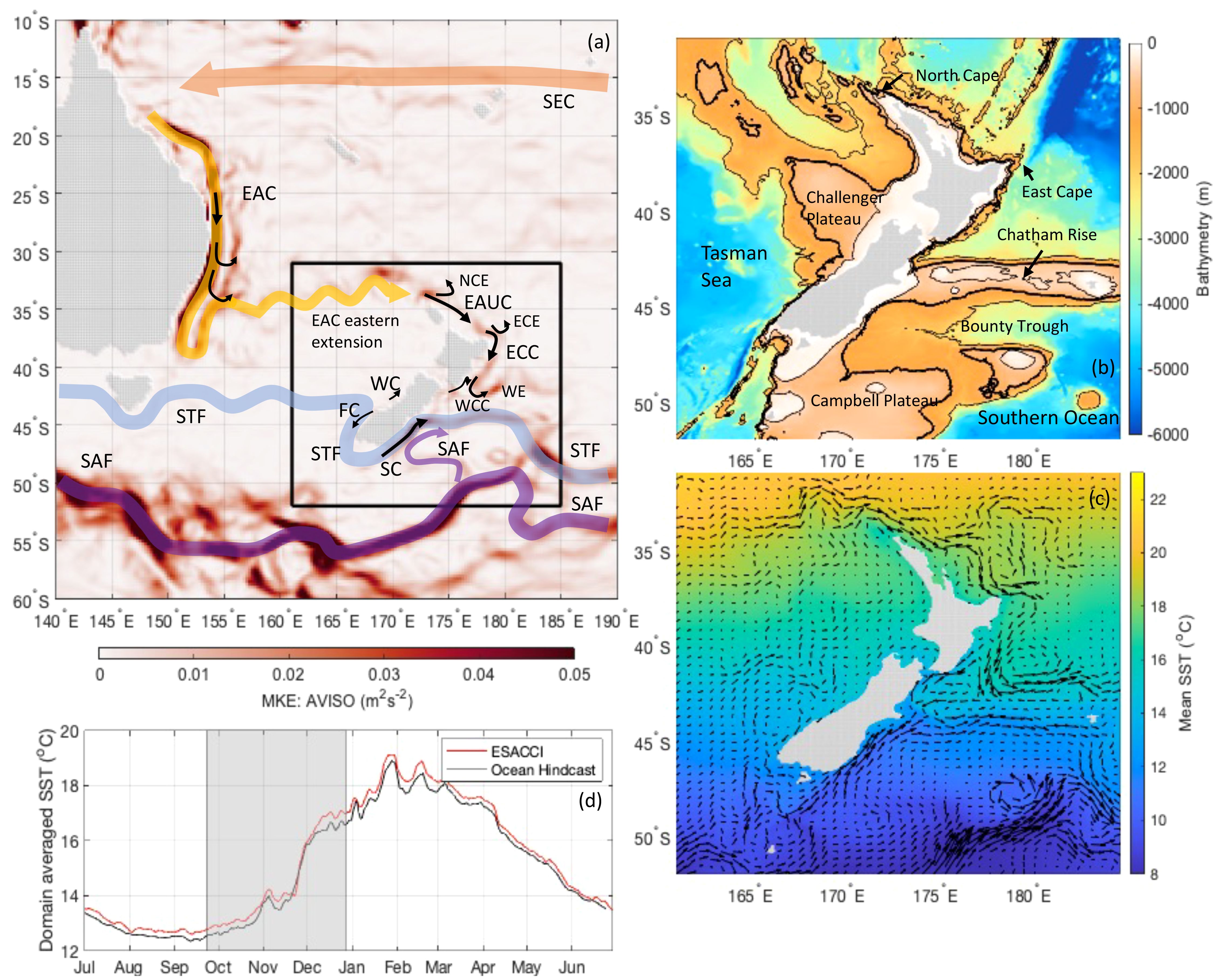
Figure 1 (A) MKE over SW Pacific with schematic of major ocean currents and fronts, and showing model domain. Current, eddy and front names are defined in Kerry et al. (2023a) (B) Model bathymetry with 400,1000,2000 m contours (1000m contour in bold) and bathymetric features labelled. (C) Mean SST with mean surface current velocity vectors from daily-average output from the Moana Ocean Hindcast. (D) Time series of the domain-averaged SST for the Moana Ocean Hindcast and observations (ESA CCI) for the year 2017-2018 and the OSSE period (grey shading).

We use a series of Observing System Simulation Experiments (OSSEs) to quantify the impact of the FVON on ocean state estimates of NZ’s shelf seas. The experiments are based on the Moana Ocean Hindcast (Azevedo Correia de Souza et al., 2022) and use 4-Dimensional Variation Data Assimilation [4D-Var Moore et al. (2004); Di Lorenzo et al. (2007); Moore et al. (2011c)] to combine the model with available observations to generate an estimate of the ocean state that is better than either alone. 4D-Var uses the (linearized) model dynamics to solve for increments in the initial conditions, atmospheric forcing, and boundary conditions, such that the modelled ocean state better fits and is in balance with the observations. We perform a series of data assimilating experiments covering the 3-month period over the onset of the 2017-2018 Tasman Sea MHW [23 Sept 2017 to 28 Dec 2017, Figure 1D; Kajtar et al. (2022)]. The goal of this paper is twofold, 1) to demonstrate the influence of subsurface temperature observations by comparing different data densities and 2) to compare different data assimilation configurations in order to improve the influence of the subsurface observations in the model.

The OSSE methodology and data assimilation system configuration are described in Section 2. The results are then presented in Section 3; we begin by presenting a domain-wide overview of the OSSEs’ performance in Section 3.3, and then we focus on the Shelf Seas (water depths shallower than 1000 m) in Section 3.4. Section 4 discusses specifics of the regional processes. Results are discussed in Section 5 in the context of ocean observing strategies and assimilation system development for shelf seas.

2 Materials and methods

2.1 Observing system simulation experiment methodology

In a realistic prediction system, a background numerical model is combined with ocean observations to produce an ocean state estimate that better represents the observations (the Analysis). The background numerical model has uncertainties associated with the initial conditions, boundary and surface forcing, and model physics. The goal of data assimilation is to combine the model with ocean observations, such that the model represents the observations (taking into account their associated errors). The resultant ocean state estimate has reduced uncertainty and provides initial conditions for the subsequent forecast (Figure 2, top). Assessing the performance of a realistic prediction system is limited by the fact that the true ocean state is not known away from the observed locations. In some cases, observations are withheld from the assimilation process for verification (e.g. Kerry et al., 2016; Zuo et al., 2019).

Figure 2

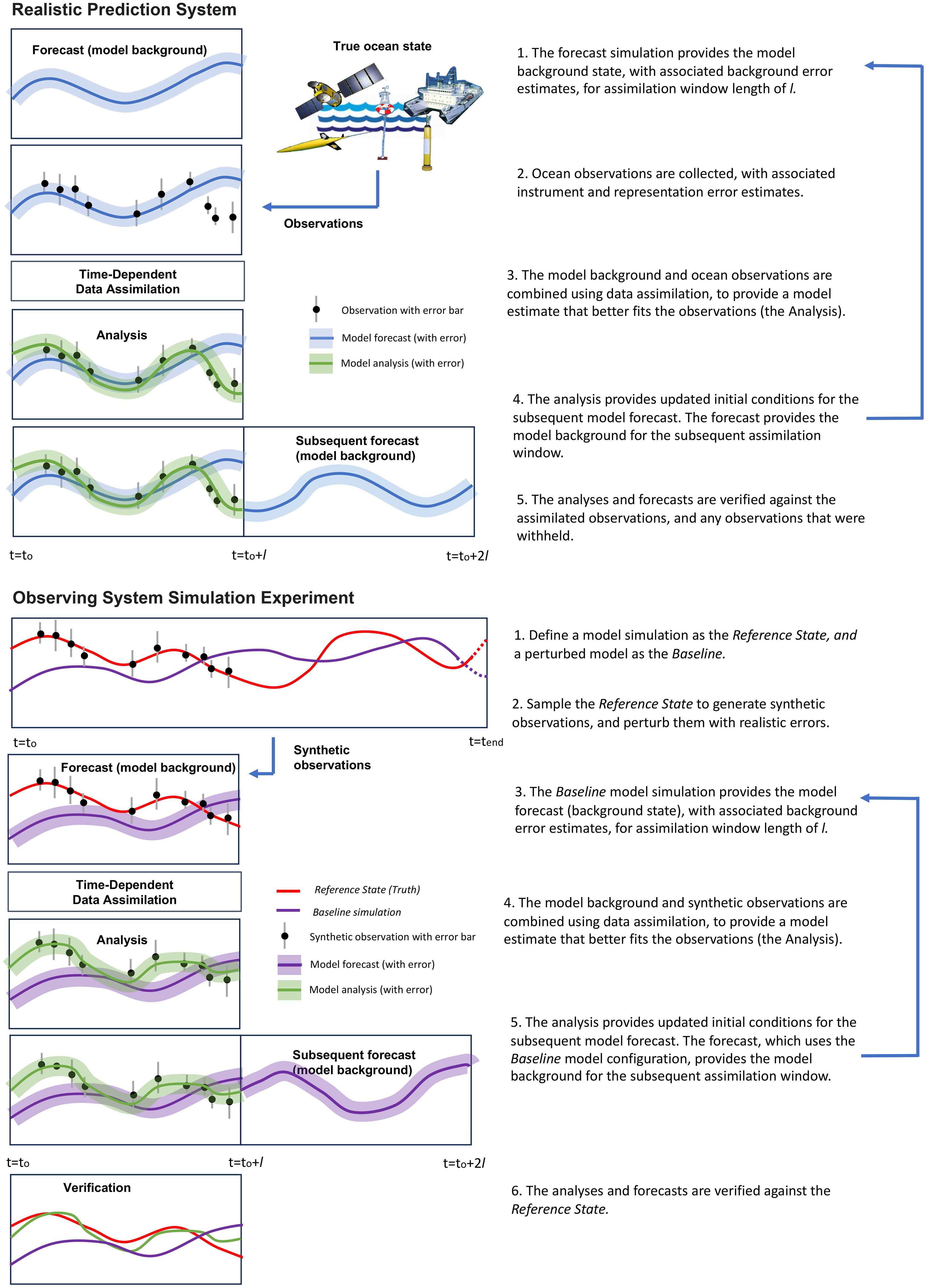
Figure 2 An outline of the steps taken in (top) a realistic prediction system and (bottom) an Observing System Simulation Experiment.

OSSEs are designed to replicate a realistic prediction system, and they have the advantage that the system can be evaluated based on a known ocean state (Figure 2, bottom). In an OSSE, a given model solution is defined as the Reference State (sometimes referred to as the Nature run). The goal is to assimilate synthetic observations extracted from the Reference State into a Baseline model (sometimes referred to as a Twin). The Baseline model is designed to represent the background numerical model from a realistic prediction system, by intentionally introducing errors in the initial conditions, boundary and surface forcing. Some OSSEs may also use a different (coarser) model resolution, and include different model physics (e.g. Halliwell et al., 2017). Because the complete ocean state is known, OSSEs allow us to rigorously compare different observing platforms and difference assimilation system configurations. OSSEs have been used widely across the atmospheric and ocean prediction communities as a relatively straight-forward and cost effective way to assess the impact of potential new observing systems (e.g. Masutani et al., 2010; Hoffman and Atlas, 2016; D’addezio et al., 2019), alternate deployments of existing systems such as observing different regions or at different sampling frequencies (e.g. Gwyther et al., 2022, 2023b), different data assimilation schemes or configurations (e.g. Moore et al., 2020; Storto et al., 2020) and resolving different physical processes (e.g. Kerry and Powell, 2022). The OSSE design used in this study is described in the following sections.

2.1.1 Reference state

The Reference State simulation used in this study is a realistic free-running model simulation that was performed from 1 July 2017 to 30 Jun 2018 with the same configuration as the Moana Ocean Hindcast (Azevedo Correia de Souza, 2022). The numerical model is configured using the Regional Ocean Modeling System (ROMS) version 3.9 to simulate the atmospherically-forced eddying ocean circulation in the NZ oceanic region. ROMS is a free-surface, hydrostatic, primitive equation ocean model solved on a curvilinear grid with a terrain-following vertical coordinate system (Shchepetkin and McWilliams, 2005). The Moana Ocean Hindcast configuration has a 5km horizontal resolution and 50 vertical s-layers. Initial and boundary conditions are from the GLORYS ocean reanalysis (Lellouche et al., 2021), developed by the Copernicus Marine Environment Monitoring Service (CMEMS). This reanalysis product was found to be the most suitable in the NZ region (Azevedo Correia de Souza et al., 2021). Atmospheric forcing fields from the Climate Forecast System Reanalysis (CFSR) provided by National Center for Atmospheric Research (NCAR) (https://climatedataguide.ucar.edu/climate-data/climate-forecast-system-reanalysis-cfsr) are used to compute the surface wind stress and surface net heat and freshwater fluxes using the bulk flux parameterization of Fairall et al. (1996). A thorough description of the model configuration and validation is presented in Azevedo Correia de Souza et al. (2022). The model provides a realistic representation of the surface and subsurface variability around NZ, and represents NZ’s major boundary currents well (Kerry et al., 2023a).

2.1.2 Baseline

As mentioned above and outlined in Figure 2, synthetic observations extracted from the Reference State are assimilated into a Baseline model. In this case, our Baseline model uses the same model grid, model physics, boundary conditions and surface forcing as the Reference State simulation; however the Baseline model is initialized from a perturbed state about the Reference State. We shift the initial conditions of the Reference State simulation by eighteen days to generate the Baseline model initial conditions. This temporal shift is chosen based on the autocorrelation of UOHC, where it takes eighteen days to reach an autocorrelation of 0.5 for UOHC (defined in Equation 3 below) at chosen points in NZ’s shelf seas. The autocorrelation analysis is described in more detail in Kerry et al. (2022) (their Figure 2).

Time-series of the Root Mean Squared Difference (RMSD) between the Reference State and the Baseline (Figures 3A–C) confirm that the chosen perturbation of eighteen days is appropriate. The plots show no convergence over the 1-year simulation, indicating that the initial conditions continue to dominate, rather than the boundary or atmospheric forcings, and that data assimilation is required to correct the ocean state estimates. The differences between the Reference State and Baseline (Figures 3D–O) are representative of typical errors in a realistic forecast system, therefore the Baseline provides a useful model in which to assimilate the synthetic observations to assess the effectiveness of the observations in improving model estimates. By only perturbing the initial conditions, our OSSEs are assessing the ability of the assimilation system to improve model state estimates (assuming perfect boundary and surface forcing).

Figure 3

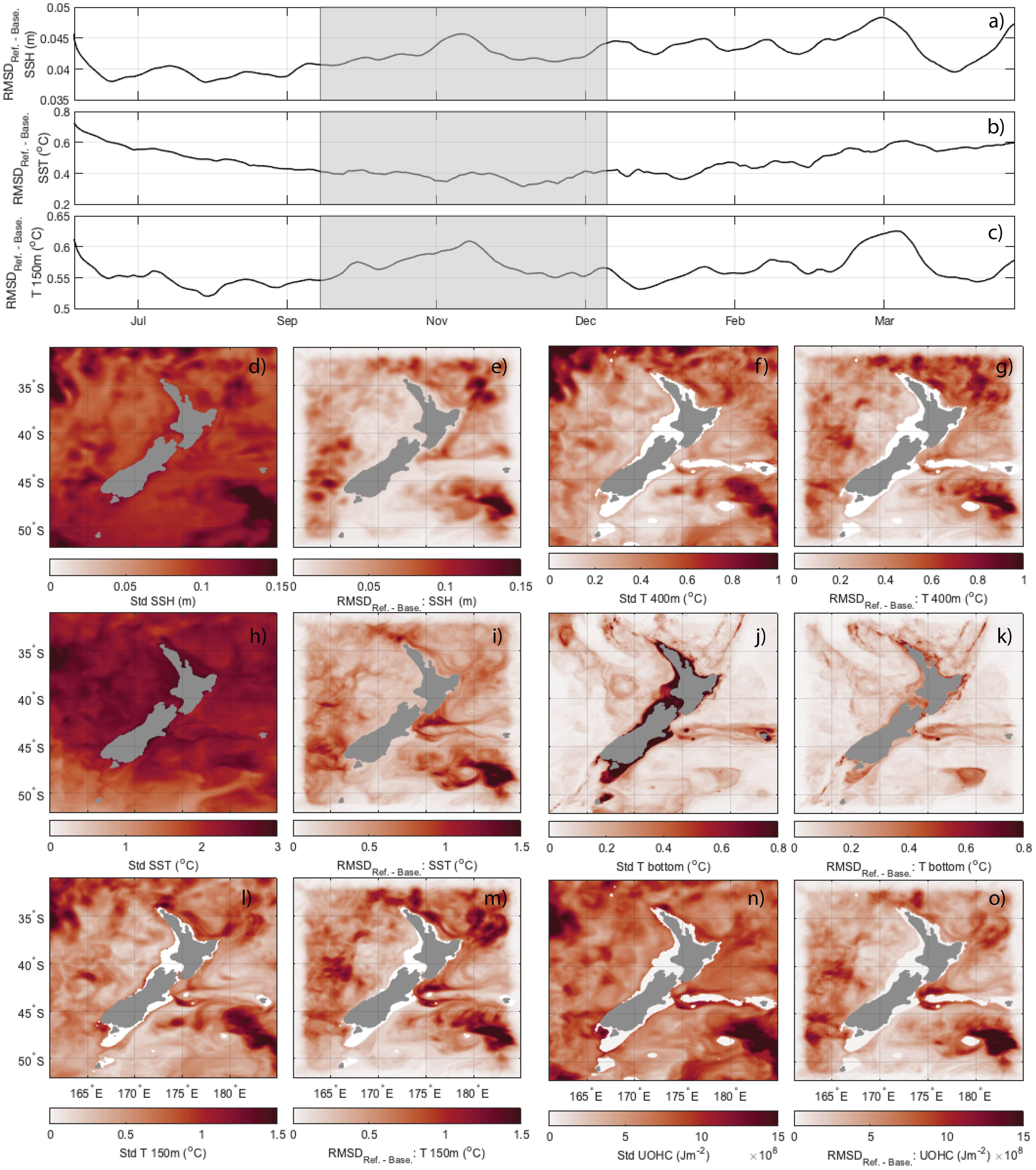
Figure 3 Time-series of domain-averaged RMSD between Reference State and Baseline State for (A) SSH, (B) SST and (C) temperature at 150 m. Standard deviation of Reference State and RMSD between Reference State and Baseline State over the full year of 2017-2018, for (D, E) SSH, (H, I) SST, (L, M) temperature at 150 m, (F, G) temperature at 400 m, (J, K) bottom temperature, and (N, O) UOHC (as defined in Section 3.2).

2.2 Experiments

In order to assess the impact of the subsurface temperature observations from fishing vessels, we performed experiments that assimilate synthetic observations that are representative of the timing, locations and associated errors of the realistic observations that were available in the region. We perform five experiments, which we describe below and in Table 1:

1. Surface only

2. Surf + FVON2021 0.2

3. Surf + FVON2022 0.2

4. Surf + FVON2022 0.1

5. Surf + FVON2022 0.2 reduced L_h

Table 1

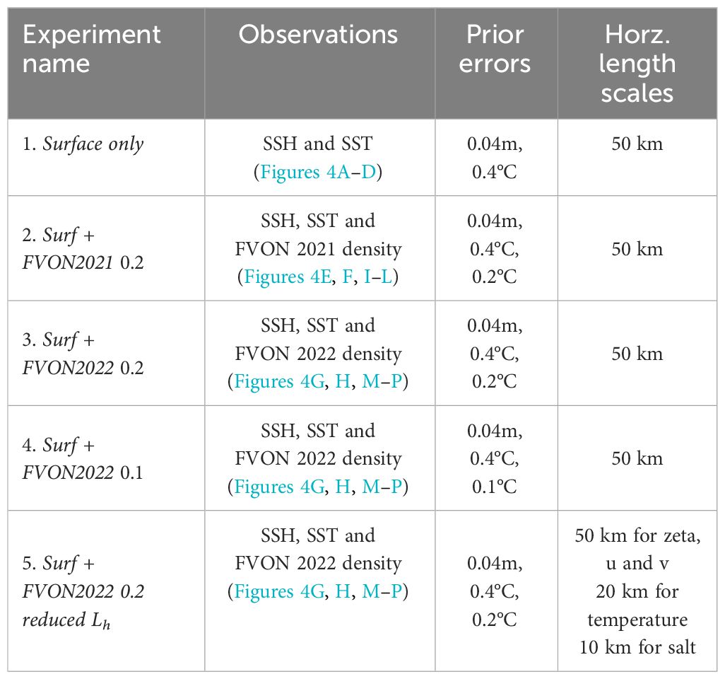
Table 1 Overview of the OSSE experiments, showing the assimilated observations, the corresponding prior observation uncertainty estimates (R), and the horizontal decorrelation lengths scales used to estimate B.

The first experiment (Surface only) assimilates only along-track SSH and gridded SST observations. The second experiment (Surf + FVON2021 0.2) assimilates surface observations as well as synthetic subsurface observations that represent the data density from the FVON that were available from 23 Sept 2021 to 28 Dec 2021, during the beginning of the Fishing Vessel sensor program. For experiments 3-5 (Surf + FVON2022 0.2, Surf + FVON2022 0.1, and Surf + FVON2022 0.2 reduced L_h), we use synthetic subsurface observations that represent the data density from the FVON available from 23 Sept 2022 to 28 Dec 2022, twelve months later, where there was an approximately 6-fold increase in observation density compared to the same period in 2021 (refer to Figure 4).

Figure 4

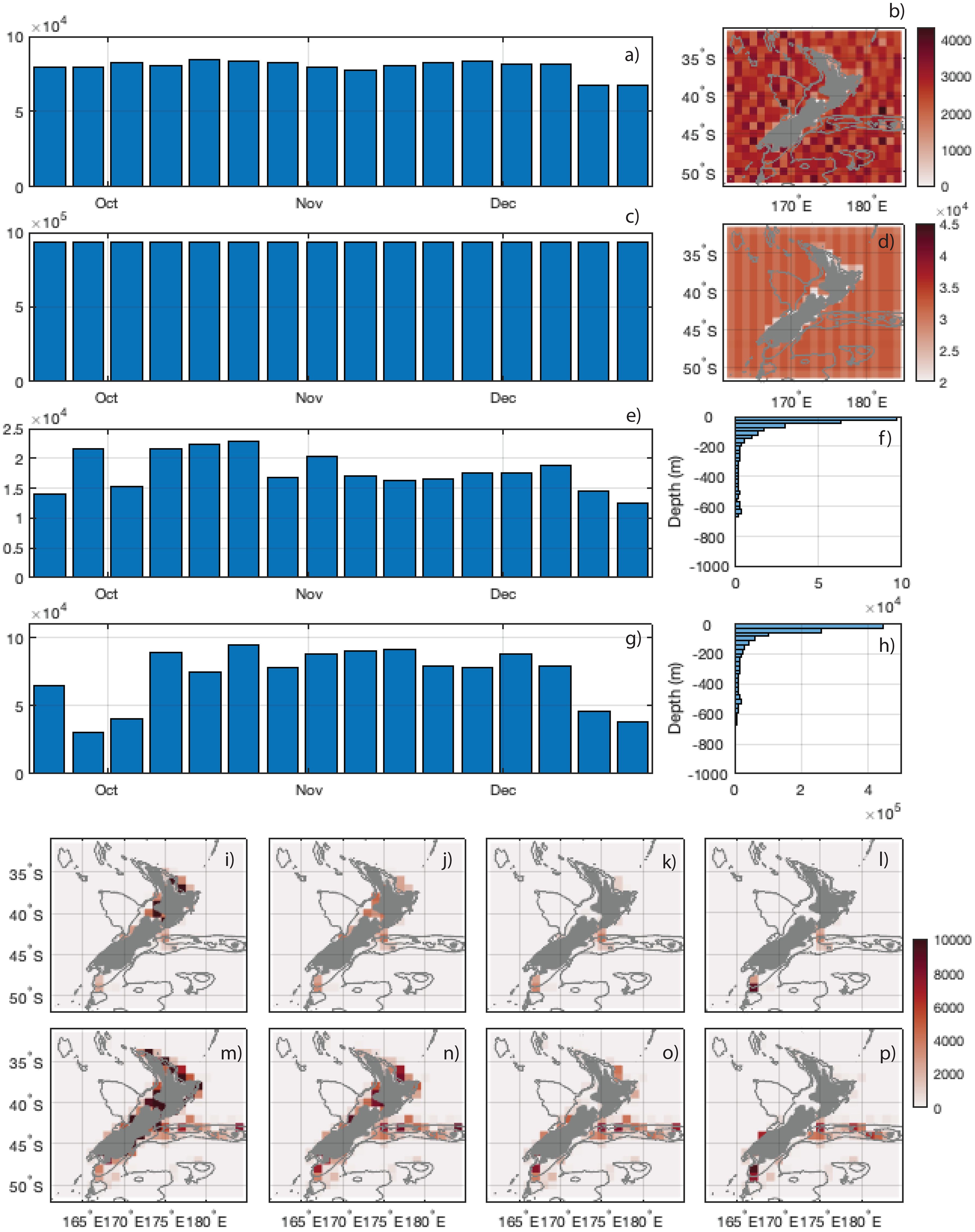
Figure 4 (A) Total number of SSH observations per 6-day window (including repeated tracks), (B) Total number of observations per 1 degree box over the OSSE period for SSH, (C) same as (A) but for SST, (D) same as (B) but for SST, (E) total number of FVON2021 observations, (F) histogram of FVON2021 observations with depth for all observations over OSSE period, (G) same as (E) but for FVON2022 observations, (H) same as (F) but for FVON2022 observations. Total number of subsurface observations per 1 degree box over the OSSE period for FVON2021 OSSE from 0-50m (I), 50-150m (J), 150-400m (K), 400-1000m (L). The same for the FVON2022 OSSE from 0-50m (M), 50-150m (N), 150-400m (O), 400-2000m (P).

In addition to testing the data densities we also compare different data assimilation configurations. In experiments 3-5, the 0.2 and 0.1 refer to the observation error estimates assigned to the subsurface temperature observations (in °C) that are specified prior to data assimilation. These prior observation errors, specified in R, are important scaling factors in the cost function (described in Equation 1 below) to avoid over-fitting to uncertain observations. Observational errors are assumed to be Gaussian with zero mean and variance given by the diagonal of the matrix R. In particular, the observational error variances for subsurface temperature observations in experiments Surf + FVON2021 0.2, Surf + FVON2022 0.2, Surf + FVON2022 0.2 reduced L_h, (Surf + FVON2022 0.1) are specified to be (0.2 °C)² [(0.1 °C)²]. Additionally it is necessary to prescribe an estimate of the uncertainties associated with the background model state, referred to as the background error covariance matrix B (as described in Equation 1 below). The uncertainties specified in B permit larger adjustments where the model is uncertain and penalize adjustments where the model errors are expected to be low. Experiments 1-4 use the same background error covariances, while for Experiment 5 the horizontal length scales used to compute the background error covariances were modified (refer to Equation 2). Details of the experiments are given in Table 1. The observations, their preprocessing and the prior observation error covariance specification are outlined in Sections 2.3 and 2.4.2 below. The formulation of the prior background error covariances is described in Section 2.4.3 and Equation 2.

The OSSE experiments are performed for the period from 23 Sept 2017 to 28 Dec 2017. This captures a period where temperatures in the Tasman Sea are close to climatology, followed by the rapid onset of the extreme MHW of summer 2017-2018, which began mid-November 2017 (Kajtar et al., 2022). The onset of the MHW is represented well in the Reference State simulation, as seen by the comparison of the domain averaged SST from the model and the European Space Agency Climate Change Initiative (ESACCI) SST data (Figure 1D). The data assimilation is performed for 6-day cycles (refer to Section 2.4.1); 16 successive 6-day cycles are performed to cover the 3-month OSSE period.

2.3 Observations

Synthetic observations are extracted, by sampling the Reference State, to represent realistic observation platforms. The synthetic observations are representative of the timing, locations and associated errors of the realistic observations that were available in the region. To be representative of realistic ocean observations, the values sampled from the Reference State at the observation times and locations are perturbed with a random error such that the errors are normally distributed within the bounds of the observational error estimates of the actual observations.

We extract synthetic observations from the Reference State to represent satellite derived along track SSH data from the Radar Altimeter Database System (RADS, Naeije et al. (2000); Figures 4A, B) and satellite derived SST data from the Operational Sea Surface Temperature and Ice Analysis (OSTIA, Donlon et al. (2012); Figures 4C, D). SSH tracks are repeated 2 hours before and after their actual time to ensure the SSH information is projected into the baroclinic ocean, rather than the fast-moving barotropic. Repeating the tracks a few hours either side of their actual time is standard practice in 4D-Var DA (e.g. Powell et al., 2009); given that 4D-Var uses the model dynamics to compute the increment adjustments, if the altimeter tracks are not repeated they can be fit as a barotropic signal. We make the valid assumption that the slow moving mesoscale circulation varies little over the +/- 2 hours. The OSTIA SST product has a 0.05° x 0.05° horizontal grid resolution and is applied daily.

The synthetic subsurface observations were extracted to represent the timing and locations of the FVON observations that were available in 2021, from 23 Sept 2021 to 28 Dec 2021, (Surf + FVON2021 0.2) and in 2022 (when data density was six-fold higher) from 23 Sept 2022 to 28 Dec 2022 (Surf + FVON2022 0.2, Surf + FVON2022 0.1, and Surf + FVON2022 0.2 reduced L_h), both in position and depth extent. Figure 4 shows the number of observations per 6-day window (Figures 4E, G) and the observation density for various depth bins (Figures 4I–P), for the FVON for 2021 and 2022 respectively.

2.4 Data assimilation configuration

2.4.1 4D-Var configuration

4D-Var uses variational calculus to solve for increments in model initial conditions, boundary conditions, and forcing such that the differences between the observations and the new model trajectory is immunized – in a least-squares sense – over a specific assimilation window. The goal is for the model to represent all of the observations in time and space using the physics of the model, and accounting for the uncertainties in the observations and background model state, producing a description of the ocean-state that is dynamically balanced and a complete solution of the non-linear model equations.

This is achieved by minimizing an objective cost function, J, that measures normalized deviations of the modelled ocean state (given the increment adjustments to model initial conditions, boundary conditions, and forcing) from the observations as well as from the modelled background state (the model prior). The cost function is a function of the increment vector and can be written as

$\begin{array}{ll}J(\delta z)=\frac{1}{2}\sum _{i=0}^n{(G\delta z-d_i)}^T{R}_i^{-1}(G\delta z-d_i)+\frac{1}{2}{(\delta z)}^T{B}^{-1}(\delta z)=J_o+J_b& (1)\end{array}$

where G = H_iM(t_i,t₀), M(t_i,t₀) represents the tangent linear version of the nonlinear model equations ℳ, integrated from t₀ to t_i. The difference between the modelled background state and the observations is represented by the innovation vector, given at each time t_i by d_i = y_i − H_i(X_f(t_i)); where y are the observations and H_i is the operator that samples the background circulation to observation points in space and time. As such, the Gδz − d_i term represents the difference between the model and the observations given the increment adjustment integrated through the tangent linear model. R is the observation error covariance matrix and B is the background error covariance matrix. In practice, with 4D-Var, subsequent integrations of the adjoint and tangent linear models (in the inner loops) are performed to solve for an increment vector that minimizes (or acceptably reduces) J. The non-linear model trajectory is updated in the outer loops.

In our experiments we assimilate observations over 6-day cycles. We employ 10 inner loops and a single outer loop in order to achieve a reasonable computational cost with an acceptable reduction in J. Initial conditions for the subsequent 6-day forecast are taken from the end of the previous analysis.

For a thorough description of the 4D-Var formulation, the reader is referred to Moore et al. (2011c). The ROMS 4D-Var implementation is well described by Moore et al. (2011c, 2011a, 2011b), and it has been used successfully in many applications [e.g., Di Lorenzo et al. (2007); Powell and Moore (2008); Powell et al. (2008); Broquet et al. (2009); Matthews et al. (2012); Zavala-Garay et al. (2012); Janeković et al. (2013); Souza et al. (2014); Kerry et al. (2016); Gwyther et al. (2022); Wilkin et al. (2022)].

2.4.2 Prior observation uncertainty assumptions

The 4D-Var method aims to solve for the nonlinear ocean solution that better represents the observations and is free within the uncertainties in the system. As such, specification of the prior observation and model background uncertainties is important. These uncertainties are prescribed in the observation error covariance matrix R and the background error covariance matrix B, respectively, and are important scaling factors in the cost function, J (Equation 1).

The prior observation uncertainties are specified as a standard deviation associated with each observation, and must account for the instrument or product error associated with the observations and the errors of representativeness. Errors of representativeness describe uncertainties due to the spatial and temporal discretization in the model; for example, if several observations exist in the same grid cell taken within the same time-step, the error of representativeness is computed by the variance of these coinciding observations. Errors of representativeness must also account for any physical processes that may be sampled by the observations but that are not resolved in the model; remotely generated internal tides is an example of these (e.g. Kerry and Powell, 2022).

In these experiments we specify prior observation errors of 0.04 m for the alongtrack SSH data and 0.4 °C for SST observations. Modern altimeter missions maintain a typical accuracy of 0.03 m for sea level (Schrama et al., 2000); for the alongtrack SSH observations, we apply an uncertainty value of 0.04 m. The alongtrack resolution is of the same order as the model horizontal resolution so errors of representativeness are low. Errors associated with representation of the surface and internal tide expression and the inverse barometer effect are expected to be small and captured within the 0.04 m. For SST, the OSTIA product provides quantified error estimates of 0.4 °C (Donlon et al., 2012). As the errors of representativeness are expected to be small as the model horizontal resolution is of the same order as the OSTIA product resolution, we specify a prior observation error of 0.4 °C for SST data. As introduced in Section 2.2, the observation error estimates assigned to the subsurface temperature observations for Surf + FVON2021 0.2, Surf + FVON2022 0.2, Surf + FVON2022 0.2 reduced L_h, (Surf + FVON2022 0.1) are specified to be 0.2 °C (0.1°C). For consistency checks associated with these prior uncertainty choices, refer to Section 3.1 and Table 2 below.

Table 2

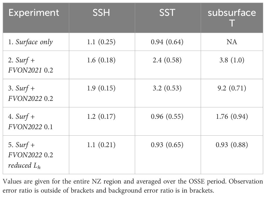
Table 2 Ratio of diagnostic and prior observation and background errors as per Desroziers’ equations (Desroziers et al., 2005).

2.4.3 Prior background uncertainty assumptions

The background error covariance matrix should represent the expected uncertainties in the model initial conditions, surface and boundary forcings. For the initial conditions and boundary forcing, the control variables are zeta (sea level), temperature, salinity and velocities (u and v). The control variables for surface forcing are surface heat flux, surface salinity flux and surface wind stress (u and v). In practice B is an NxN matrix, where N is the size of the state vector (which includes every model state variable at every grid cell, every boundary variable and every surface forcing variable). This B matrix is much too large to compute or store, and instead we estimate B by factorization, as described in Weaver and Courtier (2001), such that,

$\begin{array}{ll}B=K_b\text{ΣΛ}{L}_v^{1/2}{L}_h{L}_v^{1/2}\text{ΛΣ}{K}_b^T,& (2)\end{array}$

where K_b is the balance operator, Σ and Λ are the diagonal matrices of the background error standard deviations and normalization factors respectively, and L_v and L_h are the univariate correlations in the vertical and horizontal directions. We only prescribe univariate covariance in K_b. The dynamics are coupled through the use of the tangent linear and adjoint models in the assimilation, but not in the statistics of B. The correlation matrices, L_v and L_h, and the normalization factors, Λ, are computed as solutions to diffusion equations following Weaver and Courtier (2001). The background error standard deviations, Σ, are computed from a long free running model simulation; the natural standard deviations of the model fields are scaled to give an appropriate match between the prior specified and diagnostic background errors [as per Desroziers et al. (2005)].

The characteristic length scales chosen for L_v and L_h are assumed to be homogeneous and isotropic. The choice of horizontal length scales (detailed in Table 1) is 50 km for SSH, temperature, salinity and velocities for Experiments 1-4. For Experiment 5, the horizontal decorrelation length scales for temperature and salinity are reduced to 20 km and 10 km, respectively. The reduction in length scales for temperature and salinity was motivated by the coastal nature of the subsurface observations, where length scales of variability are typically small, compared to offshore regions dominated by mesoscale eddies (of scales of 100-200 km). Various approaches for estimating horizontal length scales are presented in Wilkin et al. (2002); Matthews et al. (2011); Kerry et al. (2016). It is noted that horizontal decorrelation length scales are likely to vary considerably across the domain given the varying circulation regions (Kerry et al., 2022). For example, for boundary currents the cross-shelf decorrelation lengths scales will be shorter than those in the alongshore direction (e.g. Oke and Sakov, 2012). Vertical isotropic decorrelation length scales are set to 30 m for all variables for all experiments. Analysis of mooring and glider observations across the south-east Australian continental shelf and into the deep ocean (detailed in Kerry et al. (2016)) find vertical decorrelation length scales range from 15-200 m for temperature, salinity and velocities, highlighting the drawbacks of specifying a single value in a DA configuration.

3 Results

3.1 Consistency of prior and posterior uncertainties

The analysis generated by the 4D-Var system is dependent on the prior assumptions of the background and observation uncertainties, and the validity of these assumptions is important in determining the optimality of the analysis. Our goal is to generate a new time-varying ocean state estimate that is a complete solution of the ocean model equations and better fits the observations, taking into account the uncertainties of both the model background state (the initial estimate, or the forecast) and the observations. A measure of the consistency of the assimilation system given the prior uncertainty assumptions can be made using a set of diagnostics based on the innovation statistics, presented in Desroziers et al. (2005). These diagnostics are based on the observation minus background, observation minus analysis, and analysis minus background differences and provide a check of the consistency of the prior choices of the background and observation error covariances. The level of agreement between the a priori specified error variances (B and R), and those diagnosed a posteriori following the methods introduced by Desroziers et al. (2005) (hereafter referred to as the diagnostic errors) provides a measure of the appropriateness of the estimates of B and R.

For all five experiments (Table 1) we present the ratio of the diagnostic observation errors and prior observation errors (and the diagnostic background errors and the prior background errors) in Table 2. The ratios are given in terms of the standard deviations (the square root of the variances) and are time-averaged over the OSSE period. A value of unity represents optimal consistency between the prior uncertainty choices and the diagnostic errors. For SSH the prior and diagnostic observation errors are typically consistent, while the prior specified background error variances for SSH are underestimated. For SST, the prior and diagnostic observation errors are consistent (values close to unity) for experiments Surface only, Surf + FVON2022 0.1, and Surf + FVON2022 0.2 reduced L_h. For experiments Surf + FVON2021 0.2 and Surf + FVON2022 0.2, diagnostic SST observation errors are elevated by 240% and 320%, respectively, compared to the prior error estimates indicating under-fitting to SST. For subsurface temperature, when prior observation errors are specified to be 0.2°C with horizontal decorrelation length scales of 50 km for temperature and salinity in B (experiments Surf + FVON2021 0.2 and Surf + FVON2022 0.2) the diagnostic errors exceed the prior specified observation errors by 380% for the 2021 density observations (Surf + FVON2021 0.2) and 920% for the 2022 density observations (Surf + FVON2022 0.2). Reducing the prior specified observation errors to 0.1°C resulted in improved consistency of the errors, but degradation of various circulation metrics (Sections 3.3 and 3.4). Experiment Surf + FVON2022 0.2 reduced L_h gave the best consistency of error estimates across the board and the best representation of surface and subsurface metrics (Sections 3.3 and 3.4).

3.2 Circulation metrics

To illustrate the impact of assimilating observations we present comparisons between the Reference State, the Baseline, and the data assimilation experiments 1-5 (Table 1). Spatial plots of the Root Mean Squared Difference (RMSD) between the Reference State and the comparison simulations are presented for the following metrics; SSH, SST, temperature at 50 m, temperature at 150 m, temperature at 400 m, temperature at 1000 m, bottom temperature, and upper ocean heat content (UOHC). The depth of 150 m represents the mean thermocline depth across the domain (Kerry et al., 2023a). The UOHC quantifies the heat carried in the upper ocean, and is given by:

$\begin{array}{ll}{\displaystyle {\int }_{\zeta -z_T}^{\zeta }{C}_p\rho (z)T(z)dz}& (3)\end{array}$

where ζ is the height of the free-surface, −z_T is the depth of the upper layer and C_p is the specific heat of sea water in J(kgK)⁻¹. In this work we define the depth of the upper layer as the 90th percentile thermocline depth computed from a long-term hindcast simulation as in Kerry et al. (2023a).

3.3 Domain-wide overview

Because we are using OSSEs, we can compare the ocean state estimates from each data assimilating experiment with a known ocean state (the Reference State). To provide a domain-wide overview of the OSSE performance we compare the representation of eight different metrics that were introduced in Section 3.2. Figures 5 and 6 display the variability (standard deviations over the OSSE period) and the differences between the experiments spatially, averaged in time over the OSSE period. The metrics are (Figure 5 rows 1-4) SSH, SST, temperature at 50 m and temperature at 150 m, and (Figure 6 rows 1-4) temperature at 400 m, temperature at 1000 m, bottom temperature, and UOHC. The columns of the figures are explained by the points below:

● Column 1: The standard deviation of the metric in the Reference State. This displays the typical variability of the metric.

● Column 2: The RMSD between the Reference State and the Baseline. This describes the magnitude by which the Reference State deviates from the Baseline (as described in Section 2.1.2 and Figure 3).

● Column 3: Red indicates improvement (lower RMSD with the Reference State) for Surf + FVON2022 0.2 reduced L_h compared to the RMSD between the Baseline and the Reference State. Blue indicates degradation. That is, the red regions demonstrate the improvement achieved by assimilation for Surf + FVON2022 0.2 reduced L_h compared to no data assimilation.

● Column 4: Red (blue) indicates improvement (degradation) given assimilation of the subsurface temperature observations (Surf + FVON2022 0.2 reduced L_h) compared to Surface only.

● Column 5: Red (blue) indicates improvement (degradation) given an increase in observation density for 2021 to 2022 (with the observation and background errors kept constant).

● Column 6: Red (blue) indicates improvement (degradation) given an increase in prior observation errors for subsurface temperature from 0.1°C to 0.2°C (with the observation platform and background errors kept constant).

● Column 7: Red (blue) indicates improvement (degradation) given a reduction in the horizontal length scales applied to temperature and salinity in the background error covariance matrix (with the observation platform and prior observation errors kept constant).

Figure 5

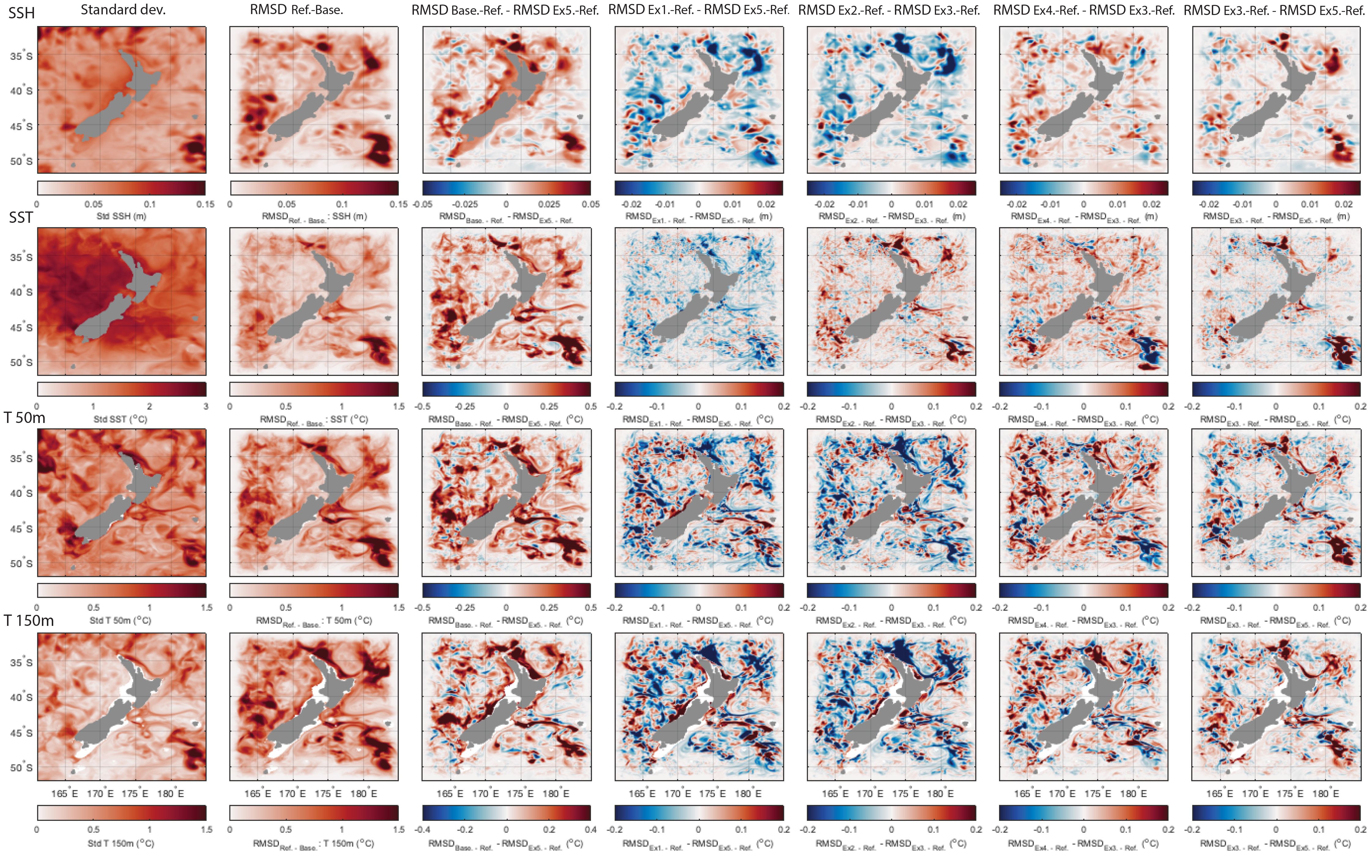
Figure 5 (Column 1) Standard deviation of Reference State, (Column 2) RMSD between Reference State and Baseline, (Column 3) difference between RMSD between Reference State and Baseline and RMSD between Reference State and Surf + FVON2022 0.2 reduced L_h, (Column 4) difference between RMSD between Reference State and Surface only and RMSD between Reference State and Surf + FVON2022 0.2 reduced L_h, (Column 5) difference between RMSD between Reference State and Surf + FVON2021 0.2 and RMSD between Reference State and Surf + FVON2022 0.2, (Column 6) difference between RMSD between Reference State and Surf + FVON2022 0.1 and RMSD between Reference State and Surf + FVON2022 0.2, and (Column 7) difference between RMSD between Reference State and Surf + FVON2022 0.2 and RMSD between Reference State and Surf + FVON2022 0.2 reduced L_h. For columns 3-7 red areas represent improvement (i.e. lower RMSD with the Reference State) for the second experiment. Rows are for SSH, SST, temperature at 50 m and temperature at 150 m. Experiments are numbered 1-5 as detailed in Table 1.

Figure 6

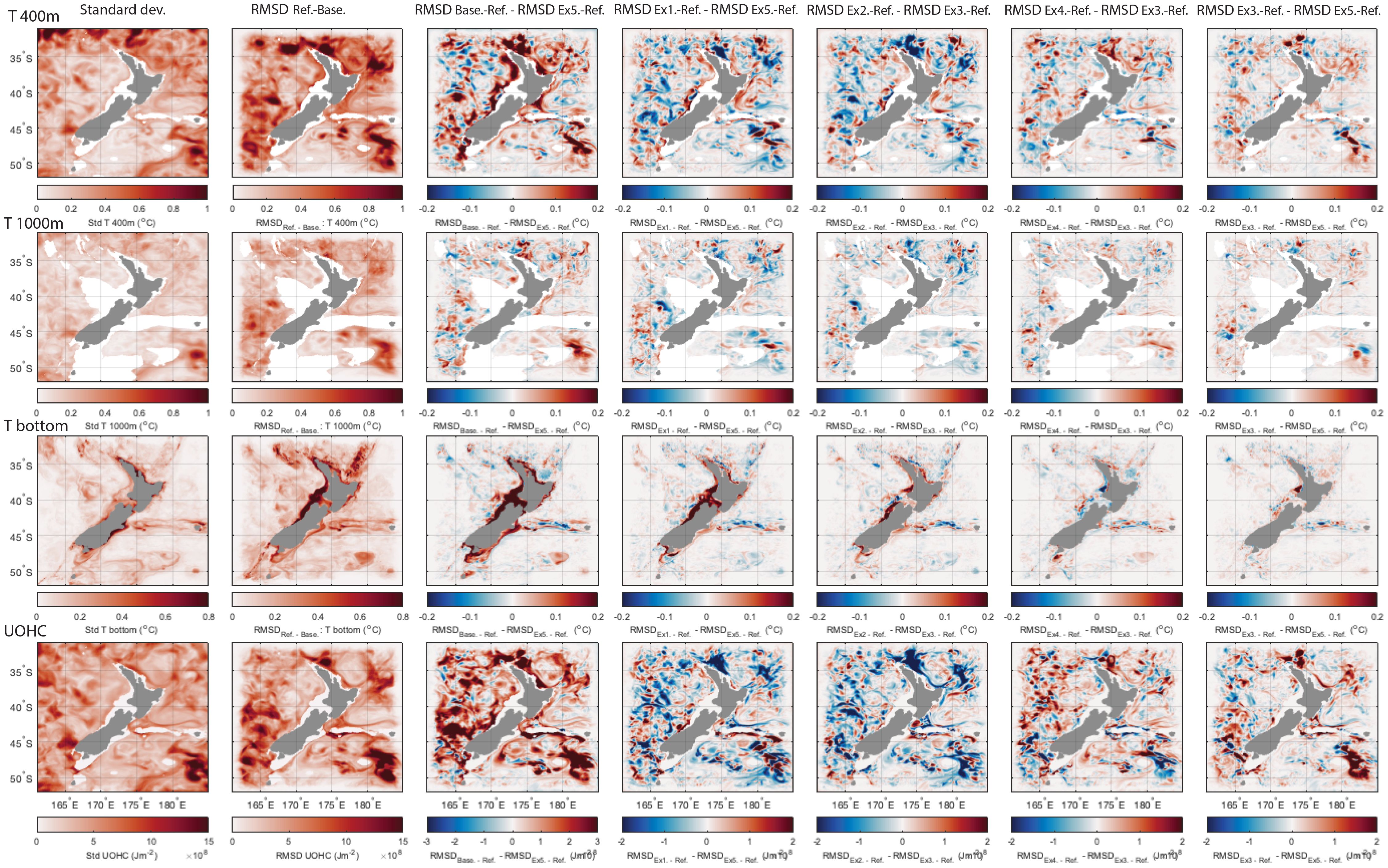
Figure 6 (Column 1) standard deviation of Reference State, (Column 2) RMSD between Reference State and Baseline, (Column 3) difference between RMSD between Reference State and Baseline and RMSD between Reference State and Surf + FVON2022 0.2 reduced L_h, (Column 4) difference between RMSD between Reference State and Surface only and RMSD between Reference State and Surf + FVON2022 0.2 reduced L_h, (Column 5) difference between RMSD between Reference State and Surf + FVON2021 0.2 and RMSD between Reference State and Surf + FVON2022 0.2, (Column 6) difference between RMSD between Reference State and Surf + FVON2022 0.1 and RMSD between Reference State and Surf + FVON2022 0.2, and (Column 7) difference between RMSD between Reference State and Surf + FVON2022 0.2 and RMSD between Reference State and Surf + FVON2022 0.2 reduced L_h. For columns 3-7 red areas represent improvement (i.e. lower RMSD with the Reference State) for the second experiment. Rows are for temperature at 400 m, temperature at 1000 m, bottom temperature and UOHC. Experiments are numbered 1-5 as detailed in Table 1.

Overall we show that experiment Surf + FVON2022 0.2 reduced L_h improves on all metrics compared to the Baseline (Column 3 of Figures 5, 6). Surface only outperforms Surf + FVON2022 0.2 reduced L_h over much of the domain for surface properties (SSH and SST) and near surface temperature (Column 4 of Figure 5), while Surf + FVON2022 0.2 reduced L_h provides improvement to temperature at 400 m outside of the North Cape/northern East Auckland Current (EAUC) region and improvement of bottom temperature over the shelf seas (Column 4 of Figure 6). A less tight fit to surface and near surface properties occurs as the system is also fitting to temperature in the lower water column. Note that Surf + FVON2022 0.2 reduced L_h stills provides a considerable improvement to surface and near surface properties and UOHC compared to the Baseline (Column 3 of Figures 5, 6).

Increasing the density of the subsurface temperature observations from Surf + FVON2021 0.2 to Surf + FVON2022 0.2 (Figures 4E–P) results in a better fit to SST, but some larger differences with the Reference State for SSH, subsurface temperature and UOHC, particularly in the EAUC region (Column 5 of Figures 5, 6). Noticeable improvement below the surface is achieved for bottom temperature (Column 5, row 3 of Figure 6). Increasing the prior specified observation uncertainties for the subsurface temperature observations from 0.1°C in Surf + FVON2022 0.1 to 0.2 °C in Surf + FVON2022 0.2 results in improvements across all metrics over most of the domain (Column 6 of Figures 5, 6). Most notably, UOHC, which integrates upper ocean properties, is degraded by introducing subsurface observations and increasing their density (Figure 6, row 4, columns 4 and 5). This degradation is due to over-fitting of the coastal temperature observations and is most pronounced in the EAUC region where cross-shelf spatial scales of variability are short. Both increasing the prior observation uncertainty estimates for subsurface temperature observations and reducing their length scales of influence provided improvements to heat content estimates (Figure 6, row 4, columns 6 and 7).

Significant improvements across all metrics were achieved by keeping the prior subsurface temperature observation errors set to 0.2°C, and adjusting the horizontal length scales used in the specification of B (refer to Section 2.4.3) in Surf + FVON2022 0.2 reduced L_h. The improvements for Surf + FVON2022 0.2 reduced L_h compared to Surf + FVON2022 0.2 are shown (by the red regions) in Column 7 of Figures 5 and 6. Adjusting the length scales provided a more consistent match between the prior and diagnostic temperature errors (Table 2, compare Experiments 4 and 5, Section 3.1), consistent with a more optimal system resulting in improved representation of surface and subsurface temperature and heat content.

3.4 Shelf seas

For a clearer view of the impacts of data assimilation on the representation of shelf seas, we now focus on the shelf regions with water depths less than 1000 m. This is where most of the subsurface FVON observations are taken, and where ocean predictions are most sought after to support fisheries and coastal users.

3.4.1 Temporal evolution of spatially-averaged errors

The temporal evolution of the errors in the shelf regions shows how the errors are reduced with the introduction of data assimilation in the different experiments (Figure 7). As discussed in Section 2.2 and Figure 1D, the OSSE period is chosen to represent a warming event, with an associated sharp rise in SST, bottom temperature and ocean heat content in NZ’s shelf seas (as shown by the spatially-averaged values for depths less than 1000 m in the Reference State, Figure 7). For all OSSEs, errors in SSH and SST are reduced most rapidly over the first 2-3 assimilation cycles (12-18 days, Figures 7A, B). The lowest errors in SSH and SST are achieved with Surface only or the less dense subsurface observations (Surf + FVON2021 0.2), followed by the dense subsurface observations with adjusted decorrelation length scales (Surf + FVON2022 0.2 reduced L_h). For bottom temperature in the shallow regions (depths less than 400 m, Figure 7C), assimilating denser subsurface observations (Surf + FVON2022 0.2, Surf + FVON2022 0.1, and Surf + FVON2022 0.2 reduced L_h) results in greater error reduction over the first 48 days, after which the OSSE with less dense subsurface observations (Surf + FVON2021 0.2) reaches similar error reduction. As the warming event intensifies (after Nov 11), both Surface only and Surf + FVON2021 0.2 provide a comparable representation of heat content in water depths less than 400 m, compared to the experiments with denser subsurface temperature observations (Figure 7D). At the peak of the warm event (after Dec 11), heat content in shallow regions is best estimated by the experiments with dense subsurface observations (Surf + FVON2022 0.2 and Surf + FVON2022 0.2 reduced L_h). Surf + FVON2022 0.2 reduced L_h provides the lowest errors across all metrics over the entire experiment period.

Figure 7

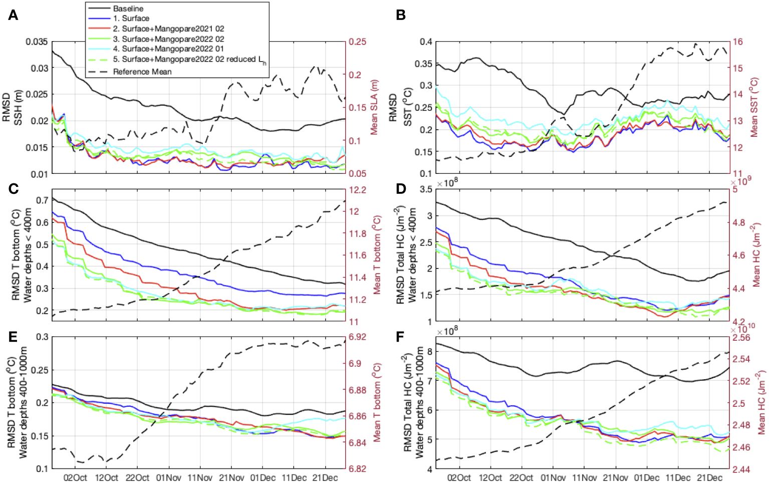
Figure 7 Time-series of RMSD between Reference State and Baseline (black), and the Reference State and the 5 OSSE experiments for the OSSE period. SSH (A) and SST (B) are for points with water depths<1000 m. Bottom temperature (C, E) and total heat content (D, F) are presented for all points with water depths<400 m and water depths from 400-1000 m. The right axes show the mean values in the Reference State simulation, illustrating the warming event.

3.4.2 Spatial maps of temporally-averaged errors

Spatial maps of the temporally-averaged errors reveal where improvements are made given the different experiments. Figure 8 shows the magnitude of the RMSD between the Baseline and the Reference State and the 5 OSSEs and the Reference State for SST, bottom temperature and heat content. Errors between the Baseline and the Reference State for SST are greatest along the shelf region influenced by the eddydominated EAUC, and along the Chatham Rise, while bottom temperature is most poorly represented along the west coast shelf in water depths less than 400 m. Heat content is most poorly represented over the plateaus and on the narrow shelf of the North Island. While the magnitudes shown in Figure 8 are useful to quantify the uncertainty associated with each model experiment, the key differences between the experiments are more clearly shown in Figures 9 and 10, where (as in Section 3.3) the differences in the temporally-averaged RMSD values are shown. Note that panel (a) represents the magnitude of the standard deviations, while for panels (b-h), red areas represent improvement (i.e. lower RMSD with the Reference State) for the second experiment, and blue represents degradation.

Figure 8

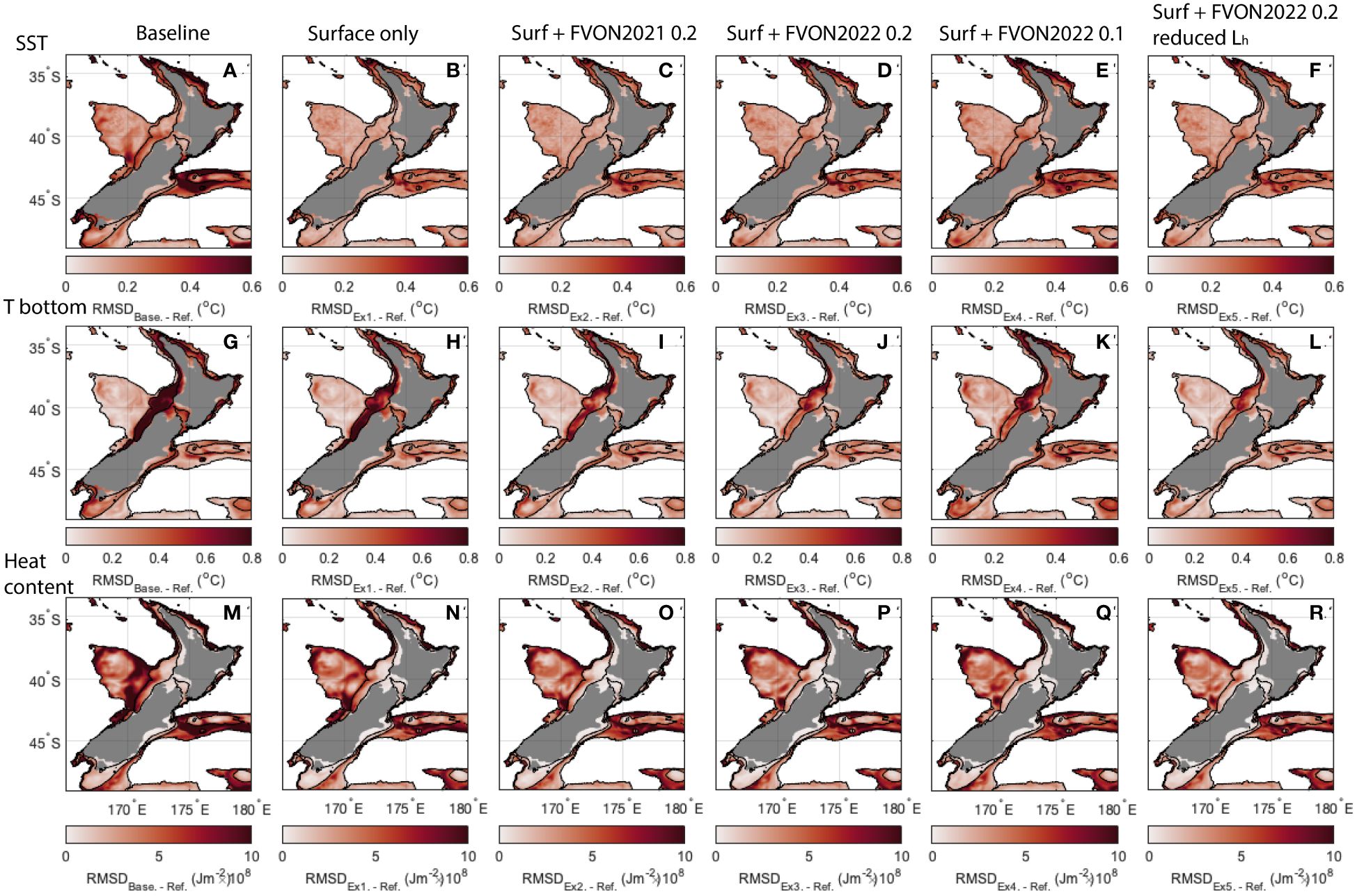
Figure 8 RMSD between the Reference State and the Baseline and the Reference State and the 5 OSSEs for (A–F) SST, (G–L), bottom temperature, and (M–R) heat content, shown for coastal regions (water depths<1000 m). 100 m, 400 m and 1000 m bathymetry contours are shown. Experiments are numbered 1-5 as detailed in Table 1.

Figure 9

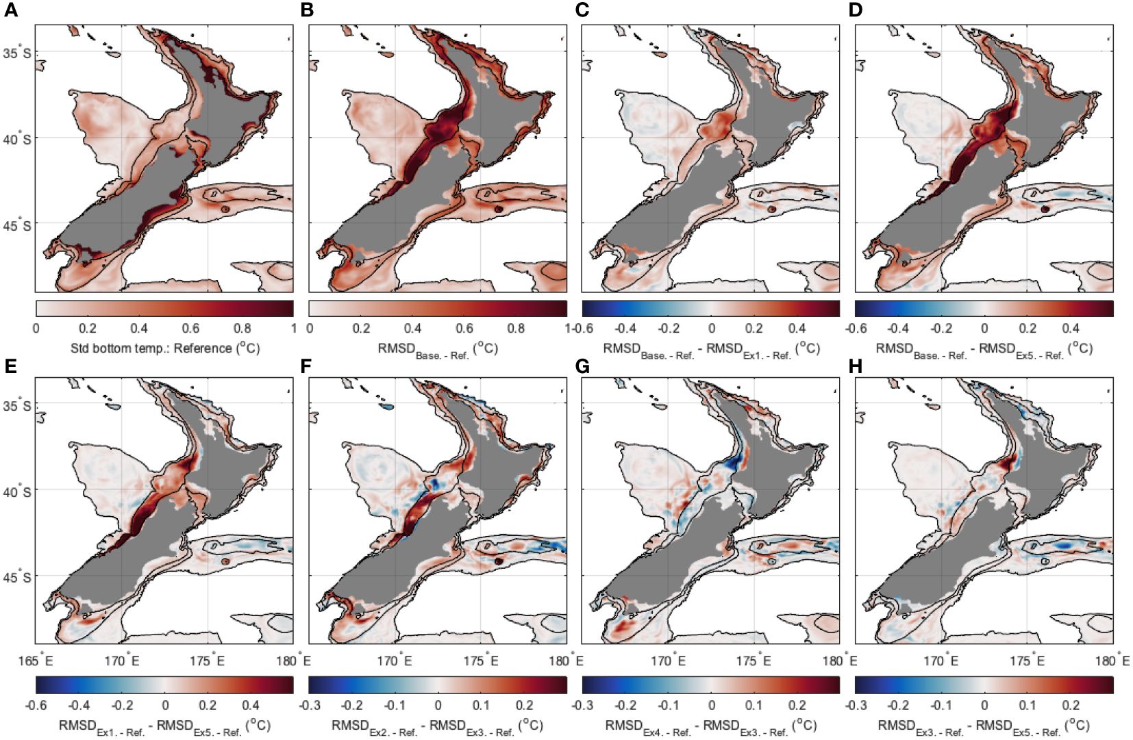
Figure 9 Bottom temperature presented for coastal regions (water depths<1000 m). (A) Standard deviation of Reference State, (B) RMSD between Reference State and Baseline, (C) difference between RMSD between Reference State and Baseline and RMSD between Reference State and Surface only, (D) difference between RMSD between Reference State and Baseline and RMSD between Reference State and Surf + FVON2022 0.2 reduced L_h, (E) difference between RMSD between Reference State and Surface only and RMSD between Reference State and Surf + FVON2022 0.2 reduced L_h, (F) difference between RMSD between Reference State and Surf + FVON2021 0.2 and RMSD between Reference State and Surf + FVON2022 0.2, (G) difference between RMSD between Reference State and Surf + FVON2022 0.1 and RMSD between Reference State and Surf + FVON2022 0.2, and (H) difference between RMSD between Reference State and Surf + FVON2022 0.2 and RMSD between Reference State and Surf + FVON2022 0.2 reduced L_h. For (B–H), red areas represent improvement (i.e. lower RMSD with the Reference State) for the second experiment. 100 m, 400 m and 1000 m bathymetry contours are shown. Experiments are numbered 1-5 as detailed in Table 1.

Figure 10

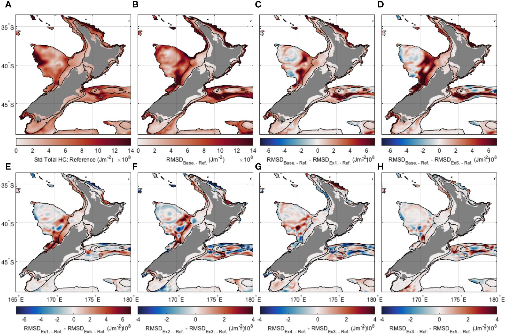
Figure 10 Total heat content presented for coastal regions (water depths<1000 m). (A) Standard deviation of Reference State, (B) RMSD between Reference State and Baseline, (C) difference between RMSD between Reference State and Baseline and RMSD between Reference State and Surface only, (D) difference between RMSD between Reference State and Baseline and RMSD between Reference State and Surf + FVON2022 0.2 reduced L_h, (E) difference between RMSD between Reference State and Surface only and RMSD between Reference State and Surf + FVON2022 0.2 reduced L_h, (F) difference between RMSD between Reference State and Surf + FVON2021 0.2 and RMSD between Reference State and Surf + FVON2022 0.2, (G) difference between RMSD between Reference State and Surf + FVON2022 0.1 and RMSD between Reference State and Surf + FVON2022 0.2, and (H) difference between RMSD between Reference State and Surf + FVON2022 0.2 and RMSD between Reference State and Surf + FVON2022 0.2 reduced L_h. For (B–H), red areas represent improvement (i.e. lower RMSD with the Reference State) for the second experiment. 100 m, 400 m and 1000 m bathymetry contours are shown. Experiments are numbered 1-5 as detailed in Table 1.

Bottom temperature estimates are improved, compared to the Baseline, when Surface only observations are assimilated (Figure 9C). Further improvements of up to 0.4°C are achieved for bottom temperature for Surf + FVON2022 0.2 reduced L_h compared to Surface only (Figure 9E), most notably along the west coast shelf region. Increasing the subsurface temperature observation density (from Surf + FVON2021 0.2 to Surf + FVON2022 0.2) gave improvements across most of the shelf sea regions corresponding to a widespread increase in subsurface temperature observations across the shelf seas (Figure 4), with the greatest improvement of up to 0.3°C being off the west coast (Figure 9F). Changes to bottom temperature representation were relatively small with adjustments to prior observation uncertainties (Figure 9G) and changes to the length scales (Figure 9H).

Heat content represents an integration of density and temperature throughout the water column (Equation 3). While the assimilation of subsurface observations (Surf + FVON2022 0.2 reduced L_h compared to Surface only) shows the greatest improvement to bottom temperature inshore of the 400 m depth contour (Figure 9E), the improvements to heat content extend offshore of the 400 m isobath (Figure 10E). This is most noticeable on the central west coast region where the extent of the heat content improvement extends considerably further offshore than the coverage of the subsurface observations (Figures 4M–P). Increasing the observation density (Surf + FVON2021 0.2 to Surf + FVON2022 0.2, Figure 10F) gives a significant improvement in heat content representation, highlighting the importance of dense subsurface temperature observations on both bottom temperature and heat content estimates in shelf seas.

The experiments that adjust the assimilation system’s prior uncertainty estimates have a less pronounced impact on bottom temperature and heat content estimates in the shelf seas (Figures 9G, H, 10G, H), compared to the impact of increasing observation density (Figures 9E, F, 10E, F). However, the differences are seen in other surface and near-surface metrics. The prior observation and background uncertainty estimates control how the assimilated observations are projected onto the unobserved portion of the ocean state, and therefore their correct specification is key to the representation of the ocean away from observed locations. This is particularly important where off-shelf water masses impact on shelf circulation, as is discussed for the EAUC region in Section 4.

3.4.3 Summary

In Table 3 we quantify the improvements of the five experiments compared to the Baseline. The results show that Surf + FVON2022 0.2 reduced L_h provides the best overall improvement across all metrics.

Table 3

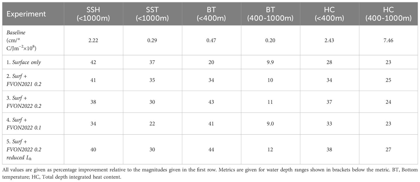
Table 3 Time-average of spatially-averaged RMSD between Baseline and Reference State, and percentage improvement of each OSSE relative to the Baseline.

4 Regional processes

Given the variety of oceanic processes across the NZ region (e.g. Chiswell et al., 2015; Fernandez et al., 2018; Stevens et al., 2019) and the variability in FVON coverage (Figure 4), improvements in model state estimates for the different OSSEs vary across the regions. In this section we discuss the differing processes at play across the NZ region in relation to the impact of the FVON and the data assimilation system, with implications for MHW predictability. The discussion draws on two previous studies that characterize the temporal and spatial scales of heat content variability around NZ (Kerry et al., 2023a) and reveal the varying drivers of MHW events across the regions (Kerry et al., 2022).

The north east coast of the North Island is dominated by mesoscale eddies associated with the EAUC and the East Cape Current (ECC) (Fernandez et al., 2018; Stevens et al., 2019). The North Cape and East Cape regions are associated with eddy separation and the formation of the North Cape Eddy (NCE) and the East Cape Eddy (ECE, Figure 1). Errors in SSH between the Reference State and the Baseline are elevated along the path of these boundary currents, and SST errors are elevated off North Cape (Figure 5, Column 2), consistent with high SST variability in this region that is poorly resolved by satellite products (Kerry et al., 2023a). Along the EAUC’s path, and in the region where it separates from East Cape, subsurface temperature and UOHC errors are elevated in the Baseline model (Figures 5 and 6, Column 2). Assimilating subsurface temperature observations that are concentrated along the narrow shelf (compared to Surface only observations) results in degradation of surface and subsurface temperature in the depth range of the mesoscale circulation (above 1000 m) and UOHC off North Cape and East Cape (Figures 5, 6, Column 4). Increasing the subsurface temperature observation density results in further degradation to SSH, subsurface temperature and UOHC, particularly off North Cape (Figures 5, 6, Column 5). We show that improved representation of SSH, SST, subsurface temperature and UOHC along the path of the EAUC and in these separation regions is achieved by relaxing the errors associated with FVON observations (Figures 5, 6, Column 6) and reducing the length scales of variability associated with the prior specified background errors (Figures 5, 6, Column 7). This highlights the importance of correctly configuring the assimilation system to prevent overfitting to dense coastal observations for the representation of boundary currents and mesoscale eddies that dominate the off-shelf circulation. This is a challenge for boundary current regions with narrow shelfs where high variability in horizontal and vertical decorrelation length scales are likely. As UOHC along the narrow shelf is modulated by the mesoscale eddies (Kerry et al., 2023a), their correct representation (offshore of the shelf) is key to predicting temperature and UOHC on the shelf. UOHC in the Bay of Plenty is driven by onshore flow associated with an eddy-dipole, and MHW events in the region are driven by anomalously high onshore heat transport down to 1000 m depth (Kerry et al., 2022). MHW prediction in the region therefore requires correct representation of the heat associated with the mesoscale eddies that are responsible for advecting heat onto the shelf.

Another notable region of elevated errors between the Baseline and the Reference State is the south west of NZ (most clearly seen Figure 3E) where the Subtropical Front (STF) impinges on the Challenger Plateau (Figure 1). This entire region also afforded better representation of surface and subsurface properties with lower errors associated with FVON observations (Figures 5, 6, Column 6) and reduced length scales of variability associated with the prior background errors (Figures 5, 6, Column 7). The STF feeds the southward flowing Fiordland Current (FC) and the weaker, northward flowing Westland Current (WC, Figure 1A), although heat content over the plateau is not dominantly driven by advection (Kerry et al., 2022). On the Challenger Plateau, increased subsurface temperature observation density resulted in improved bottom temperature estimates on the shelf for depths less than 400 m (Figures 9E, F), and improved heat content estimates over the plateau for water depths from 400-1000 m (Figure 10). Kerry et al. (2022) show that heat content on the shelf off of the west coast of the South Island is sensitive to large scale adjustments in the ocean’s subsurface structure over the west coast, in contrast to other boundary current dominated regions where advection dominates. This is likely to be why the greatest improvements in subsurface temperature and UOHC representation upon assimilation of the FVON observations are seen on the shelf regions of the west coast.

The shallow region off of the southern tip of the South Island (the Stewart Plateau and Snares Shelf region) is influenced by the Fiordland Current (FC), with heat content over the shelf between positively correlated to heat content over the South Island’s west coast shelf region (Kerry et al., 2023a). Improved bottom temperature estimates in the region are seen with increased density of FVON observations (Figures 9E, F) and higher observation errors (Figure 9G).

Circulation to the east along the Chatham Rise results from the convolution of the Southland Current (SC) and the extension of the ECC as they turn eastward (Figure 1A). A westward flowing counter current returns water along the rise to form the Wairarapa Coastal Current (WCC) (Kerry et al., 2023a). Including FVON data (Figure 10E) and increasing the observation density (Figure 10F) resulted in improved UOHC representation along the Chatham Rise where this counter current exists. Anomalously high heat transport in this counter current drives MHW events in the central east coast region (Kerry et al., 2022). Improvements in representation of surface and subsurface temperature, and UOHC along the Chatham Rise are clearly seen in Figures 5 and 6, Column 3.

5 Discussion

Data assimilation is particularly challenging for coastal and shelf regions where observations are typically temporally and/or spatially sparse and where the circulation variability contains a broad range of time and space scales (e.g. Walstad and McGillicuddy, 2000; Kerry et al., 2020). Effective assimilation of subsurface observations into ocean circulation models is crucial to improving subsurface structure estimates (Gwyther et al., 2022). Here we have compared five Observing System Simulation Experiments (Table 1) to quantify the impact of assimilating fishing-vessel mounted temperature sensors that collect subsurface temperature observations in NZ’s shelf seas. We show that, not only is increased density of subsurface observations important in the representation of the subsurface ocean, their successful assimilation into an ocean model requires careful specification of the prior observation and background uncertainties to optimize the way in which the observations inform the numerical model estimates.

We show that including coastal and shelf subsurface temperature observations provides improvements in the representation of bottom temperature and heat content, most notably at water depths< 400m (Table 3). The Surface only experiment provided a 20% and 28% improvement compared to the Baseline for bottom temperature and heat content, respectively, while the experiments assimilating subsurface temperature observations provide improvements of between 34-44% and 33-38%. Increasing the density of the subsurface observations while keeping the prior specified observation and background uncertainties the same (Surf + FVON2021 0.2 to Surf + FVON2022 0.2) results in improvements in bottom temperature representation but a degradation in SSH and SST representation in the shelf seas (Table 3). This degradation is greater when a tighter fit to the subsurface observations is specified (that is, with prior observation uncertainties reduced from 0.2°C to 0.1°C, Surf + FVON2022 0.2 to Surf + FVON2022 0.1). The best fit across all metrics is Surf + FVON2022 0.2 reduced L_h, in which the prior observation uncertainties for the subsurface observations are set at 0.2°C and the decorrelation length scales for temperature and salinity specified in the background error covariance matrix are reduced from 50 km to 20 km and 10 km, respectively. Both the domain-wide view (Section 3.3) and the results focused on the shelf seas (Section 3.4), show that Surf + FVON2022 0.2 reduced L_h is the superior system in representing all of the chosen metrics. This is related to both the increased subsurface temperature observation density and the assimilation configuration. Specifically, the increase in prior observation uncertainties for the subsurface observations (from 0.1 to 0.2°C) prevents over-fitting to the dense coastal and shelf observations, and shorter horizontal decorrelation length scales associated with the background error covariance matrix allow improved projection of the observations onto the modelled state.

Previous experiments assimilating similar fishing-vessel-derived observations in the Adriatic Sea conducted by Aydoğdu et al. (2016) also highlight the value of such observations, although the observing system was simpler and only single-point vertical values were utilized instead of the profiles provided by the FVON sensors in this study. The authors emphasize the importance of domain coverage over the number of observations. From the distribution of the subsurface temperature observations presented in Figure 4 we see that, although not dramatic, there is an increase in the area covered by the FVON sensors in 2022 in relation to 2021. This factor can be important for the improved metrics discussed above. Similarly, the OSSE methodology could also be used to assess the optimum observational data density required to achieve a requisite model improvement. By starting with data in all grid cells a data thinning approach could be used in order to guide how many fishing vessels are required, or where FVON observations will have the greatest impact. In this experiment, bottom temperature in the shallow seas reaches similar error reduction for the lower density observations compared to the denser observations after two months (Figure 7C); however this corresponds to a rapid increase in bottom temperature and may be related to full water column mixing. In the EAC region, Kerry et al. (2018) show that observations taken in regions of higher variability have more impact on transport and EKE estimates throughout the current system. This is consistent with results of Gwyther et al. (2022) who show that synthetic temperature profile observations through the downstream eddy-dominated region of the EAC system are considerably more impactful in improving subsurface temperature and UOHC estimates throughout the region than the same observations taken upstream, across the mostly coherent EAC. In a similar study, weekly profiles (with profiles occurring in every assimilation cycle) are shown to provide considerably better results that fortnightly or monthly sampling (Gwyther et al., 2023b).

While our results highlight the value of subsurface temperature observations in representing bottom temperature in shelf seas, we note that correct representation of the SSH (associated with the geostrophic currents) and correct representation of temperature throughout the water column (not just at the bottom) is required to correctly estimate heat content. This requires careful design of the data assimilation system in order to achieve maximum benefit from the observing system. Specifically, the way by which information from the observations is projected onto the modelled ocean state is controlled by the background error covariance matrix, and the fit to the observations is controlled by the prior observation uncertainties. Overfitting to certain observations can result in degradation of the representation of other fields. Specifically, in this study we see that over-fitting to dense near-shore temperature profile observations is at the expense of temperature representation of offshore waters and surface and near-surface fields (as in Surf + FVON2022 0.1). This is most pronounced along the narrow shelf region, dominated by the EAUC and the ECC. Further, careful specification of the decorrelation length scales used to compute the background error covariance matrix is required (Section 2.4.3). Consistency of improvement across both surface and subsurface properties is important for correctly representing upper ocean heat content; a crucial metric for understanding and predicting MHWs (Kerry et al., 2022). Furthermore, in regions where the off-shelf circulation modulates the shelf circulation, such as the EAUC (as discussed in Section 4) and the EAC, where mesoscale eddies drive cross-shelf transport (Malan et al., 2022), correct representation of the subsurface structure offshore of the shelf is key to predicting shelf circulation. While our results focus on analysis skill, we note that preventing over-fitting is crucial to the quality of forecasts (e.g. Kerry et al., 2023b).

The assimilation of surface data alone can improve subsurface representation, yet the addition of subsurface observations has the potential to provide considerable further improvement given an effective assimilation system, as was shown in this study. The improvement of the subsurface temperature representation with assimilation of SST was shown by Zhang et al. (2010a), but they also highlight the value of subsurface glider measurements of temperature and salinity on salinity forecasts. Ezer and Mellor (1997) find assimilation of SSH data reduces errors more effectively in mid-depths (around 500 m), and SST data reduces errors in the upper layers (above 100 m), with a combination of SST and SSH data able to provide improved skill at all depths compared to assimilation of each set of data separately. Pasmans et al. (2019) find that surface observations are required in combination with the subsurface observations of temperature and salinity from gliders to prevent unphysical eddies from forming in the vicinity of the glider transects. Representer analysis by Zhang et al. (2010b) shows how the information from glider transects extends toward the dynamically upstream, yet in practice Pasmans et al. (2019) found that their assimilation of glider observations failed to produce large-scale subsurface corrections. A similar result was found in Siripatana et al. (2020), where observations from a deep water mooring array produced improvements to the representation of the EAC core depth in its vicinity, with degradation in the unobserved downstream region. Likewise, Gwyther et al. (2023a) found that eddy subsurface structure was often poorly represented in the absence of observations within the eddy. This issue was addressed in a post-processing feature mapping approach developed by Rykova (2023) in which individual ocean eddies are corrected if a profiling float exists within the feature. Each profiling float only affects the specific feature that it observes; however, this approach is yet to be implemented in an automated manner for sequential data assimilation and is limited by the fact that many features are unsampled. All of these results highlight the challenges associated with the projection of information from observed variables onto the unobserved ocean state in data assimilation systems, which is controlled by the observation-model covariances, and emphasize the importance of domain coverage.

Indeed the greatest challenges associated with assimilation of temporally and spatially sparse observations in dynamically active regions relate to the specification of the background error covariances (Moore et al., 2019). In advanced time-dependent data assimilation, the model physics constrain the state-estimates such that the prescribed covariances are propagated in time to identify observation-model covariance. In 4D-Var (and 3D-Var) the background error covariance matrix (B) is usually based on information about the dominant dynamical balances of the system, as well as information about the average statistics of errors in the forecast system (Lorenc, 2003). In classic 4D-Var, the covariances in B are assumed to be static with isotropic horizontal and vertical length scales and the tangent-linear and adjoint models introduce flow-dependence in the error covariance via the time evolution of the background. In our 4DVar configuration, we estimate B by factorization (Weaver and Courtier, 2001) and prescribe univariate covariance (the dynamics are coupled by the tangent-linear and adjoint models in the assimilation, but not in the statistics of B). On the other hand, an Ensemble Kalman Filter (EnKF) employs an ensemble of nonlinear model states to estimate B and so capture what are commonly referred to in Numerical Weather Prediction (NWP) as the “errors of the day”.

Within the scope of this study, we compare two different values of subsurface temperature prior observation uncertainties and two different decorrelation length scales associated with the background error covariance matrix. Considerable differences in the model state estimates highlight the sensitivity to these prior uncertainty estimates and the importance of their careful specification. Our NZ model covers various dynamically different circulation regimes so the length scales of variability are anisotropic. Furthermore, the subsurface observations are concentrated in coastal and shallow shelf regions. Zhang et al. (2010a) acknowledge similar limitations given the isotropic and univariate nature of B, and while multivariate background error covariance terms have been added to the ROMS 4D-Var system, they rely on the assumption of approximate geostrophic dynamics which may not be adequate for dynamic continental shelf regions. It is likely that a more optimal approach would be to estimate flow-dependent background error covariances that capture the “errors of the day”, and the spatially-varying decorrelation length scales. Ensemble-variational methods, that make use of the dynamical interpolation properties of the adjoint (4D-Var), and the explicit flow-dependent error covariances (used in ensemble methods) have been studied extensively for atmospheric DA (e.g. Lorenc et al., 2015) with improvements in forecast skill achieved particularly in dynamically active systems (Raynaud et al., 2011; Lorenc and Jardak, 2018). At the European Centre for Medium Range Weather Forecasting (Bonavita et al., 2016) and at Météo-France (Bouyssel et al., 2022), the use of flow-dependent, ensemble-based estimates to describe the background error covariance matrix at the start of the 4D-Var assimilation window has resulted in improved accuracy of the analysis and forecast fields. In the ocean, Pasmans et al. (2020) use Ensemble-4DVar in a realistic coastal ocean model and show that further research and development is required.

Accurate model estimates and forecasts of the coastal ocean provide useful information to decision-makers to effectively manage our coastal environment, mitigate risks and support industry. The importance of the subsurface structure of the circulation for ecological and economic impacts, particularly related to MHW events, has been revealed by several studies (Schaeffer and Roughan, 2017; Elzahaby and Schaeffer, 2019). Specifically, the sensitivity of MHW onset to the ocean’s subsurface structure was revealed in Kerry et al. (2022), highlighting the importance of correct subsurface representation for MHW predictability. Fishing vessels as providers of subsurface observations provide a new frontier of in situ data, particularly in coastal and shelf seas (Van Vranken et al., 2023), and we must develop the skills to effectively make use of the data to improve model estimates and predictions. Our future work aims to address the properties of the background error covariance matrix to optimize the influence of spatially and temporally inhomogeneous observations, with a focus on improving subsurface representation.

Data availability statement

The model configuration used for this study is available at Azevedo Correia de Souza (2022), https://doi.org/10.5281/zenodo.5895265. The raw data supporting the conclusions of this article will be made available by the authors, without undue reservation.

Author contributions

CK: Data curation, Formal analysis, Investigation, Methodology, Validation, Visualization, Writing – original draft, Writing – review & editing. MR: Conceptualization, Funding acquisition, Project administration, Resources, Supervision, Writing – review & editing. JS: Data curation, Investigation, Methodology, Project administration, Software, Writing – review & editing.

Funding

The author(s) declare financial support was received for the research, authorship, and/or publication of this article. This work is a contribution to the Moana Project (www.moanaproject.org), funded by the New Zealand Ministry of Business Innovation and Employment, contract number METO1801.

Conflict of interest

The authors declare that the research was conducted in the absence of any commercial or financial relationships that could be construed as a potential conflict of interest.

Publisher’s note

All claims expressed in this article are solely those of the authors and do not necessarily represent those of their affiliated organizations, or those of the publisher, the editors and the reviewers. Any product that may be evaluated in this article, or claim that may be made by its manufacturer, is not guaranteed or endorsed by the publisher.

References

Aydoğdu A., Pinardi N., Pistoia J., Martinelli M., Belardinelli A., Sparnocchia S. (2016). Assimilation experiments for the fishery observing system in the Adriatic Sea. J. Mar. Syst. 162, 126–136. doi: 10.1016/j.jmarsys.2016.03.002

CrossRef Full Text | Google Scholar

Azevedo Correia de Souza J. (2022). Moana Ocean Hindcast. doi: 10.5281/zenodo.5895265

CrossRef Full Text | Google Scholar

Azevedo Correia de Souza J., Couto P., Soutelino R., Roughan M. (2021). Evaluation of four global ocean reanalysis products for New Zealand waters–a guide for regional ocean modelling. N. Z. J. Mar. Freshw. Res. 55, 132–155. doi: 10.1080/00288330.2020.1713179

CrossRef Full Text | Google Scholar

Azevedo Correia de Souza J., Suanda A., Couto P., Smith R., Kerry C., Roughan M. (2022). Moana Ocean Hindcast - a 25+ years simulation for New Zealand waters using the ROMS v3.9 model. Geosc. Model. Dev. doi: 10.5194/egusphere-2022-41. Submitted.

CrossRef Full Text | Google Scholar

Balmaseda M., Anderson D., Vidard A. (2007). Impact of Argo on analyses of the global ocean. Geophysical Res. Lett. 34. doi: 10.1029/2007GL030452

CrossRef Full Text | Google Scholar

Bonavita M., Hólm E., Isaksen L., Fisher M. (2016). The evolution of the ECMWF hybrid data assimilation system. Q. J. R. Meteorol. Soc 142, 287–303. doi: 10.1002/qj.2652

CrossRef Full Text | Google Scholar

Bouyssel F., Berre L., Bénichou H., Chambon P., Girardot N., Guidard V., et al. (2022). “The 2020 global operational NWP data assimilation system at Météo-France,” in Data Assimilation for Atmospheric, Oceanic and Hydrologic Applications (Vol. IV). (Springer Berlin, Heidelberg), 645–664.

Google Scholar

Broquet G., Edwards C. A., Moore A., Powell B. S., Veneziani M., Doyle J. D. (2009). Application of 4D-Variational data assimilation to the California Current System. Dynam. Atmos. Oceans 48, 69–92. doi: 10.1016/j.dynatmoce.2009.03.001

CrossRef Full Text | Google Scholar

Chiswell S. M., Bostock H. C., Sutton P. J., Williams M. J. (2015). Physical oceanography of the deep seas around New Zealand: A review. N. Z. J. Mar. Freshw. Res. 49, 286–317. doi: 10.1080/00288330.2014.992918

CrossRef Full Text | Google Scholar

D’addezio J. M., Smith S., Jacobs G. A., Helber R. W., Rowley C., Souopgui I., et al. (2019). Quantifying wavelengths constrained by simulated SWOT observations in a submesoscale resolving ocean analysis/forecasting system. Ocean Model. 135, 40–55. doi: 10.1016/j.ocemod.2019.02.001

CrossRef Full Text | Google Scholar

Darmaraki S., Somot S., Sevault F., Nabat P., Cabos Narvaez W. D., Cavicchia L., et al. (2019). Future evolution of marine heatwaves in the Mediterranean Sea. Climate Dynamics 53, 1371–1392. doi: 10.1007/s00382-019-04661-z

CrossRef Full Text | Google Scholar

Desroziers G., Berre L., Chapnik B., Poli P. (2005). Diagnosis of observation, background and analysis-error statistics in observation space. Q. J. R. Meteorological Soc. 131, 3385–3396. doi: 10.1256/qj.05.108

CrossRef Full Text | Google Scholar

Di Lorenzo E., Moore A. M., Arango H. G., Cornuelle B. D., Miller A. J., Powell B. S., et al. (2007). Weak and strong constraint data assimilation in the inverse Regional Ocean Modelling System (ROMS): Development and application for a baroclinic coastal upwelling system. Ocean Model. 16, 160–187. doi: 10.1016/j.ocemod.2006.08.002

CrossRef Full Text | Google Scholar

Donlon C. J., Martin M., Stark J., Roberts-Jones J., Fiedler E., Wimmer W. (2012). The operational sea surface temperature and sea ice analysis (OSTIA) system. Remote Sens. Environ. 116, 140–158. doi: 10.1016/j.rse.2010.10.017

CrossRef Full Text | Google Scholar

Elzahaby Y., Schaeffer A. (2019). Observational insight into the subsurface anomalies of marine heatwaves. Front. Mar. Sci. 6. doi: 10.3389/fmars.2019.00745

CrossRef Full Text | Google Scholar

Elzahaby Y., Schaeffer A., Roughan M., Delaux S. (2021). Oceanic circulation drives the deepest and longest marine heatwaves in the East Australian Current System. Geophys. Res. Lett. 48. doi: 10.1029/2021GL094785

CrossRef Full Text | Google Scholar

Elzahaby Y., Schaeffer A., Roughan M., Delaux S. (2022). Why the mixed layer depth matters when diagnosing marine heatwave drivers using a heat budget approach. Front. Clim. 4. doi: 10.3389/fclim.2022.838017

CrossRef Full Text | Google Scholar

Ezer T., Mellor G. L. (1997). Data assimilation experiments in the Gulf Stream region: How useful are satellite-derived surface data for nowcasting the subsurface fields? J. Atmos. Ocean. Technol. 14, 1379–1391. doi: 10.1175/1520-0426(1997)014〈1379:DAEITG〉2.0.CO;2

CrossRef Full Text | Google Scholar

Fairall C. W., Bradley E. F., Rogers D. P., Edson J. B., Young G. S. (1996). Bulk parameterization of air-sea fluxes for tropical ocean-global atmosphere Coupled-Ocean Atmosphere Response Experiment. J. Geophys. Res. Oceans 101, 3747–3764. doi: 10.1029/95JC03205

CrossRef Full Text | Google Scholar

Fernandez D., Bowen M., Sutton P. (2018). Variability, coherence and forcing mechanisms in the New Zealand ocean boundary currents. Prog. Oceanogr. 165, 168–188. doi: 10.1016/j.pocean.2018.06.002

CrossRef Full Text | Google Scholar

Frölicher T. L., Fischer E. M., Gruber N. (2018). Marine heatwaves under global warming. Nature 560, 360–364. doi: 10.1038/s41586-018-0383-9

PubMed Abstract | CrossRef Full Text | Google Scholar

Gwyther D. E., Keating S. R., Kerry C., Roughan M. (2023a). How does 4D-Var data assimilation affect the vertical representation of mesoscale eddies? A case study with observing system simulation experiments (OSSEs) using ROMS v3. 9. Geosci. Model. Dev. 16, 157–178. doi: 10.5194/gmd-16-157-2023

CrossRef Full Text | Google Scholar

Gwyther D. E., Kerry C., Roughan M., Keating S. R. (2022). Observing system simulation experiments reveal that subsurface temperature observations improve estimates of circulation and heat content in a dynamic Western Boundary Current. Geosci. Model. Dev. 15 (17), 6541–6565. doi: 10.5194/gmd-15-6541-2022

CrossRef Full Text | Google Scholar

Gwyther D. E., Roughan M., Kerry C., Keating S. R. (2023b). Impact of assimilating repeated subsurface temperature transects on state estimates of a Western Boundary Current. Front. Mar. Sci. 9. doi: 10.3389/fmars.2022.1084784

CrossRef Full Text | Google Scholar

Haines K. (2018). Ocean reanalyses. New Front. Operational Oceanogr. 19, 545–562. doi: 10.17125/gov2018.ch19

CrossRef Full Text | Google Scholar

Halliwell G. R. Jr., Mehari M. F., Le Hénaff M., Kourafalou V. H., Androulidakis I. S., Kang H. S., et al. (2017). North Atlantic Ocean OSSE system: Evaluation of operational ocean observing system components and supplemental seasonal observations for potentially improving tropical cyclone prediction in coupled systems. J. Oper. Oceanogr. 10, 154–175. doi: 10.1080/1755876X.2017.1322770

CrossRef Full Text | Google Scholar

Hoffman R. N., Atlas R. (2016). Future observing system simulation experiments. Bull. Am. Meteorological Soc. 97, 1601–1616. doi: 10.1175/BAMS-D-15-00200.1

CrossRef Full Text | Google Scholar

Jacox M., Tommasi D., Alexander M., Hervieux G., Stock C. (2019). Predicting the evolution of the 2014-16 California Current System marine heatwave from an ensemble of coupled global climate forecasts. Front. Mar. Sci. 6. doi: 10.3389/fmars.2019.00497

CrossRef Full Text | Google Scholar

Janeković I., Powell B. S., Matthews D., McManus M. A., Sevadjian J. (2013). 4D-Var data assimilation in a nested, coastal ocean model: A Hawaiian case study. J. Geophys. Res. Oceans 118, 1–14. doi: 10.1002/jgrc.20389

CrossRef Full Text | Google Scholar

Kajtar J. B., Bachman S. D., Holbrook N. J., Pilo G. S. (2022). Drivers, dynamics, and persistence of the 2017/2018 Tasman Sea marine heatwave. J. Geophys. Res. Oceans 127, e2022JC018931. doi: 10.1029/2022JC018931

CrossRef Full Text | Google Scholar

Kerry C. G., Powell B. S. (2022). Including tides improves subtidal prediction in a region of strong surface and internal tides and energetic mesoscale circulation. J. Geophys. Res. Oceans 127, e2021JC018314. doi: 10.1029/2021JC018314

CrossRef Full Text | Google Scholar

Kerry C. G., Powell B. S., Roughan M., Oke P. R. (2016). Development and evaluation of a high-resolution reanalysis of the East Australian Current region using the Regional Ocean Modelling System (ROMS3.4) and Incremental Strong-Constraint 4-Dimensional Variational (IS4D-Var) data assimilation. Geosci. Model. Dev. 9, 3779–3801. doi: 10.5194/gmd-9-3779-2016

CrossRef Full Text | Google Scholar

Kerry C., Roughan M., Azevedo Correia de Souza J. (2022). Drivers of upper ocean heat content extremes (marine heatwaves) around New Zealand revealed by Adjoint Sensitivity Analysis. Front. Clim. 4. doi: 10.3389/fclim.2022.980990

CrossRef Full Text | Google Scholar

Kerry C., Roughan M., De Souza J. (2023a). Characterising the variability of boundary currents and ocean heat content around New Zealand using a multi-decadal high-resolution regional ocean model. J. Geophysical Res.: Oceans 128 (4), e2022JC018624. doi: 10.1029/2022JC018624

CrossRef Full Text | Google Scholar

Kerry C. G., Roughan M., Keating S., Gwyther D., Brassington G., Siripitana A., et al. (2023b). Comparison of 4-Dimensional Variational and Ensemble Optimal interpolation data assimilation systems using a Regional Ocean Modelling System (v3. 4) configuration of the eddy-dominated East Australian Current System. EGUsphere 2023, 1–40. doi: 10.5194/egusphere-2023-2355

CrossRef Full Text | Google Scholar

Kerry C. G., Roughan M., Powell B. S. (2018). Observation impact in a regional reanalysis of the East Australian Current System. J. Geophys. Res. Oceans 123 (10), 7511–7528. doi: 10.1029/2017JC013685

CrossRef Full Text | Google Scholar

Kerry C., Roughan M., Powell B. (2020). Predicting the submesoscale circulation inshore of the East Australian Current. J. Mar. Syst. 204, 103286. doi: 10.1016/j.jmarsys.2019.103286

CrossRef Full Text | Google Scholar

Lellouche J. M., Greiner E., Bourdalle-Badie R., Garric G., Melet A., Drevillon M., et al. (2021). The Copernicus global 1/12° oceanic and sea ice GLORYS12 reanalysis. Front. Earth Sci. 9. doi: 10.3389/feart.2021.698876

CrossRef Full Text | Google Scholar

Lorenc A. C. (2003). Modelling of error covariances by 4D-Var data assimilation. Q. J. R. Meteorol. Soc 129, 3167–3182. doi: 10.1256/qj.02.131

CrossRef Full Text | Google Scholar

Lorenc A. C., Bowler N. E., Clayton A. M., Pring S. R., Fairbairn D. (2015). Comparison of Hybrid-4DEnVar and Hybrid-4DVar data assimilation methods for global NWP. Monthly Weather Rev. 143, 212–229. doi: 10.1175/MWR-D-14-00195.1

CrossRef Full Text | Google Scholar

Lorenc A. C., Jardak M. (2018). A comparison of hybrid variational data assimilation methods for global NWP. Q. J. R. Meteorol. Soc 144, 2748–2760. doi: 10.1002/qj.3401

CrossRef Full Text | Google Scholar

Malan N., Roughan M., Stanley G. J., Holmes R., Li J. (2022). Quantifying cross-shelf transport in the east Australian current system: a budget-based approach. J. Phys. Oceanogr. 52, 2555–2572. doi: 10.1175/JPO-D-21-0193.1

CrossRef Full Text | Google Scholar

Masutani M., Woollen J. S., Lord S. J., Emmitt G. D., Kleespies T. J., Wood S. A., et al. (2010). Observing system simulation experiments at the National Centers for Environmental Prediction. J. Geophysical Res.: Atmos. 115. doi: 10.1029/2009JD012528

CrossRef Full Text | Google Scholar

Matthews D., Powell B. S., Janeković I. (2012). Analysis of 4-dimensional variational state estimation of the Hawaiian waters. J. Geophys. Res. Oceans 117. doi: 10.1029/2011JC007575

CrossRef Full Text | Google Scholar

Matthews D., Powell B., Milliff R. (2011). Dominant spatial variability scales from observations around the Hawaiian Islands. Deep-Sea Res. I: Oceanogr. Res. 58, 979–987. doi: 10.1016/j.dsr.2011.07.004

CrossRef Full Text | Google Scholar

Moore A. M., Arango H. G., Broquet G., Edwards C., Veneziani M., Powell B. S., et al. (2011a). The Regional Ocean Modelling System (ROMS) 4-dimensional variational data assimilation systems: Part II – Performance and application to the California Current System. Prog. Oceanog. 91, 50–73. doi: 10.1016/j.pocean.2011.05.003

CrossRef Full Text | Google Scholar

Moore A. M., Arango H. G., Broquet G., Edwards C., Veneziani M., Powell B. S., et al. (2011b). The Regional Ocean Modelling System (ROMS) 4-dimensional variational data assimilation systems: Part III – Observation impact and observation sensitivity in the California Current System. Prog. Oceanog. 91, 74–94. doi: 10.1016/j.pocean.2011.05.005

CrossRef Full Text | Google Scholar

Moore A. M., Arango H. G., Broquet G., Powell B. S., Zavala-Garay J. (2011c). The Regional Ocean Modelling System (ROMS) 4-dimensional variational data assimilation systems: Part I – System overview and formulation. Prog. Oceanog. 91, 34–49. doi: 10.1016/j.pocean.2011.05.004

CrossRef Full Text | Google Scholar

Moore A. M., Arango H. G., Di Lorenzo E., Cornuelle B. D., Miller A. J., Neilson D. J. (2004). A comprehensive ocean prediction and analysis system based on the tangent linear and adjoint of a regional ocean model. Ocean Model. 7, 227–258. doi: 10.1016/j.ocemod.2003.11.001

CrossRef Full Text | Google Scholar

Moore A. M., Martin M. J., Akella S., Arango H. G., Balmaseda M., Bertino L., et al. (2019). Synthesis of ocean observations using data assimilation for operational, real-time and reanalysis systems: A more complete picture of the state of the ocean. Front. Mar. Sci. 6. doi: 10.3389/fmars.2019.00090

CrossRef Full Text | Google Scholar

Moore A., Zavala-Garay J., Arango H. G., Edwards C. A., Anderson J., Hoar T. (2020). Regional and basin scale applications of ensemble adjustment Kalman filter and 4D-Var ocean data assimilation systems. Prog. oceanogr. 189, 102450. doi: 10.1016/j.pocean.2020.102450

CrossRef Full Text | Google Scholar

Naeije M., Schrama E., Scharroo R. (2000). “The radar altimeter database system (RADS),” in IGARSS 2000. IEEE 2000 International Geoscience and Remote Sensing Symposium. Taking the Pulse of the Planet: The Role of Remote Sensing in Managing the Environment. Proceedings (Cat. No. 00CH37120), (IEEE) Vol. 2. 487–490. doi: 10.1109/IGARSS.2000.861605

CrossRef Full Text | Google Scholar

Oke P., Sakov P. (2012). Assessing the footprint of a regional ocean observing system. J. Mar. Syst. 105, 30–51. doi: 10.1016/j.jmarsys.2012.05.009

CrossRef Full Text | Google Scholar

Oliver E. C., Donat M. G., Burrows M. T., Moore P. J., Smale D. A., Alexander L. V., et al. (2018a). Longer and more frequent marine heatwaves over the past century. Nat. Commun. 9, 1–12. doi: 10.1038/s41467-018-03732-9

PubMed Abstract | CrossRef Full Text | Google Scholar

Oliver E. C., Lago V., Hobday A. J., Holbrook N. J., Ling S. D., Mundy C. N. (2018b). Marine heatwaves off eastern Tasmania: Trends, interannual variability, and predictability. Prog. Oceanogr. 161, 116–130. doi: 10.1016/j.pocean.2018.02.007

CrossRef Full Text | Google Scholar

Pasmans I., Kurapov A., Barth J., Ignatov A., Kosro P., Shearman R. (2019). Why gliders appreciate good company: Glider assimilation in the Oregon-Washington coastal ocean 4D-Var system with and without surface observations. J. Geophys. Res. Oceans 124, 750–772. doi: 10.1029/2018JC014230

CrossRef Full Text | Google Scholar

Pasmans I., Kurapov A. L., Barth J. A., Kosro P. M., Shearman R. K. (2020). Ensemble 4D-Var (En4DVar) data assimilation in a coastal ocean circulation model. Part II: Implementation offshore Oregon–Washington, USA. Ocean Model. 154, 101681. doi: 10.1016/j.ocemod.2020.101681

CrossRef Full Text | Google Scholar

Powell B. (2017). Quantifying how observations inform a numerical reanalysis of Hawaii. J. Geophys. Res. Oceans 122, 8427–8444. doi: 10.1002/2017JC012854

CrossRef Full Text | Google Scholar

Powell B. S., Arango H. G., Moore A. M., Di Lorenzo E., Milliff R. F., Foley D. (2008). 4D-Var data assimilation in the Intra-Americas Sea with the The Regional Ocean Modelling System (ROMS). Ocean Modell. 25, 173–188. doi: 10.1016/j.ocemod.2008.04.008

CrossRef Full Text | Google Scholar

Powell B. S., Moore A. M. (2008). Estimating the 4D-Var analysis error of GODAE products. Ocean Dynamics 59, 121–138. doi: 10.1007/s10236-008-0172-3

CrossRef Full Text | Google Scholar

Powell B., Moore A., Arango H., Di Lorenzo E., Milliff R., Leben R. (2009). Near real-time ocean circulation assimilation and prediction in the Intra-Americas Sea with ROMS. Dynamics Atmos. Oceans 48, 46–68. doi: 10.1016/j.dynatmoce.2009.04.001

CrossRef Full Text | Google Scholar

Raynaud L., Berre L., Desroziers G. (2011). An extended specification of flow-dependent background error variances in the Météo-France global 4D-Var system. Q. J. R. Meteorol. Soc 137, 607–619. doi: 10.1002/qj.795

CrossRef Full Text | Google Scholar

Rykova T. (2023). Improving forecasts of individual ocean eddies using feature mapping. Sci. Rep. 13, 6216. doi: 10.1038/s41598-023-33465-9

PubMed Abstract | CrossRef Full Text | Google Scholar

Schaeffer A., Roughan M. (2017). Subsurface intensification of marine heatwaves off southeastern Australia: The role of stratification and local winds. Geophys. Res. Lett. 44, 5025–5033. doi: 10.1002/2017GL073714

CrossRef Full Text | Google Scholar

Schaeffer A., Sen Gupta A., Roughan M. (2023). Seasonal stratification and complex local dynamics control the sub-surface structure of marine heatwaves in Eastern Australian coastal waters. Commun. Earth Environ. 4, 304. doi: 10.1038/s43247-023-00966-4

CrossRef Full Text | Google Scholar

Schrama E., Scharroo R., Naeije M. (2000). Radar Altimeter Database System (RADS): Towards a Generic Multi-satellite Altimeter Database System (BCRS rapport (Netherlands Remote Sensing Board (BCRS), Programme Bureau, Rijkswaterstaat Survey Department).

Google Scholar

Shchepetkin A. F., McWilliams J. C. (2005). The Regional Oceanic Modeling System (ROMS): A split-explicit, free-surface, topography-following-coordinate oceanic model. Ocean Modell. 9, 347–404. doi: 10.1016/j.ocemod.2004.08.002

CrossRef Full Text | Google Scholar

Siripatana A., Kerry C., Roughan M., Souza J. M. A., Keating S. (2020). Assessing the impact of nontraditional ocean observations for prediction of the East Australian Current. J. Geophys. Res. Oceans 125, e2020JC016580. doi: 10.1029/2020JC016580

CrossRef Full Text | Google Scholar

Souza J., Powell B. S., Castillo-Trujillo A. C., Flament P. (2014). The vorticity balance of the ocean surface in Hawaii from a regional reanalysis. J. Phys. Oceanogr. 45, 424–440. doi: 10.1175/JPO-D-14-0074.1

CrossRef Full Text | Google Scholar

Stevens C. L., O’Callaghan J. M., Chiswell S. M., Hadfield M. G. (2021). Physical oceanography of New Zealand/Aotearoa shelf seas – a review. N. Z. J. Mar. Freshw. Res. 55 (1), 6–45. doi: 10.1080/00288330.2019.1588746

CrossRef Full Text | Google Scholar

Storto A., Alvera-Azcárate A., Balmaseda M. A., Barth A., Chevallier M., Counillon F., et al. (2019). Ocean reanalyses: Recent advances and unsolved challenges. Front. Mar. Sci. 6. doi: 10.3389/fmars.2019.00418

CrossRef Full Text | Google Scholar

Storto A., Falchetti S., Oddo P., Jiang Y.-M., Tesei A. (2020). Assessing the impact of different ocean analysis schemes on oceanic and underwater acoustic predictions. J. Geophysical Res.: Oceans 125, e2019JC015636. doi: 10.1029/2019JC015636

CrossRef Full Text | Google Scholar

Van Vranken C., Jakoboski J., Carroll J. W., Cusack C., Gorringe P., Hirose N., et al. (2023). Towards a global Fishing Vessel Ocean Observing Network (FVON): State of the art and future directions. Front. Mar. Sci. 10. doi: 10.3389/fmars.2023.1176814

CrossRef Full Text | Google Scholar

Walstad L. J., McGillicuddy D. J. (2000). Data assimilation for coastal observing systems. Oceanography 13, 47–53. doi: 10.5670/oceanog.2000.52

CrossRef Full Text | Google Scholar

Weaver A., Courtier P. (2001). Correlation modelling on the sphere using generalized diffusion equation. Quart. J. R. Meteorol. Soc 127, 1815–1846. doi: 10.1002/qj.49712757518

CrossRef Full Text | Google Scholar

Wilkin J. L., Bowen M. M., Emery W. J. (2002). Mapping mesoscale currents by optimal interpolation of satellite radiometer and altimeter data. Ocean Dynamics 52, 95–103. doi: 10.1007/s10236-001-0011-2

CrossRef Full Text | Google Scholar

Wilkin J., Levin J., Moore A., Arango H., López A., Hunter E. (2022). A data-assimilative model reanalysis of the US Mid Atlantic Bight and Gulf of Maine: Configuration and comparison to observations and global ocean models. Prog. Oceanogr. 209, 102919. doi: 10.1016/j.pocean.2022.102919

CrossRef Full Text | Google Scholar

Zavala-Garay J., Wilkin J. L., Arango H. G. (2012). Predictability of mesoscale variability in the East Australian Current given strong-constraint data assimilation. J. Phys. Ocean. 42, 1402–1420. doi: 10.1175/JPO-D-11-0168.1

CrossRef Full Text | Google Scholar

Zhang W. G., Wilkin J. L., Arango H. G. (2010a). Towards an integrated observation and modeling system in the New York Bight using variational methods. Part I: 4D-Var data assimilation. Ocean Model. 35, 119–133. doi: 10.1016/j.ocemod.2010.08.003

CrossRef Full Text | Google Scholar

Zhang W. G., Wilkin J. L., Levin J. C. (2010b). Towards an integrated observation and modeling system in the New York Bight using variational methods. Part II: Repressenter-based observing strategy evaluation. Ocean Model. 35, 134–145. doi: 10.1016/j.ocemod.2010.06.006

CrossRef Full Text | Google Scholar

Zuo H., Balmaseda M. A., Tietsche S., Mogensen K., Mayer M. (2019). The ECMWF operational ensemble reanalysis–analysis system for ocean and sea ice: a description of the system and assessment. Ocean Sci. 15, 779–808. doi: 10.5194/os-15-779-2019

CrossRef Full Text | Google Scholar