Habitat associations of marine predators in the northern California Current during the low productivity downwelling season

Bliss, Laura M.; Zamon, Jeannette E.; Davoren, Gail K.; Hanson, M. Bradley; Noren, Dawn P.; Emmons, Candice; Holt, Marla M.

doi:10.3389/fmars.2024.1355439

ORIGINAL RESEARCH article

Front. Mar. Sci., 29 April 2024

Sec. Marine Megafauna

Volume 11 - 2024 | https://doi.org/10.3389/fmars.2024.1355439

Habitat associations of marine predators in the northern California Current during the low productivity downwelling season

Laura M. Bliss^1*

Jeannette E. Zamon^1,2

¹Department of Biological Sciences, University of Manitoba, Winnipeg, Manitoba, Canada
²Northwest Fisheries Science Center, National Marine Fisheries Service, National Oceanic and Atmospheric Administration, Seattle, WA, United States

Introduction: Eastern Boundary Upwelling Systems are some of the most productive marine ecosystems in the world. Little is known about habitat associations and spatial distributions of marine predators during seasonal periods of low productivity because there are few at-sea surveys during this period. During low productivity or prey scarcity, predators consuming similar prey in the same time and space may compete for limited resources, or they may avoid competition by exploiting different habitats or occupying separate spaces (i.e. niche partitioning). In this study, we examined habitat associations and niche partitioning of marine predators during the low-productivity winter downwelling season of the northern California Current Ecosystem (CCE).

Methods: Seabird and marine mammal counts were continuously collected during systematic at-sea surveys during February–March/April in the northern California Current across four years (2006, 2008, 2009, and 2012). We examined seabird and marine mammal distributions in relation to seven habitat characteristics [i.e., sea surface temperature (°C), salinity, depth (m), seafloor slope (%), distance from shore (km), and distance from the 100 m and 200 m isobaths (km)]. We used a non-parametric multivariate analysis [i.e. canonical correspondence analysis (CCA)] to quantify species’ habitat associations and directional distribution ellipses to explore overlap in species core winter habitat.

Results: Results show 49 seabird and ten marine mammal species inhabit the CCE during this low productivity period, including endangered southern resident killer whales (Orcinus orca). Seabirds and marine mammals exhibited significant but low overlap in habitat associations (i.e. weak niche partitioning) and similar habitat associations to summer studies.

Discussion: We also found that some species with similar foraging strategies showed asymmetrical spatial range overlap (i.e. common murre (Uria aalge) and parakeet auklet (Aethia psittacula)), which may mean that expected increased competition due to climate change can negatively affect some species more than others. Given that climate change is leading to increased frequencies, intensities, and durations of marine heat waves during winter months, addressing the winter ecology knowledge gap will be important to understanding how climate change is going to affect species that reside in or migrate through the northern California Current during the low productivity downwelling season.

Introduction

Eastern Boundary Upwelling Ecosystems (EBUE) are some of the most productive marine ecosystems in the world, as these systems provide a highly disproportionate amount of marine productivity for their size (Cushing, 1971; Carr, 2001; Chavez and Messié, 2009). The California Current Ecosystem (CCE) on the west coast of North America is one of four such EBUE systems, and the CCE experiences seasonal changes in primary and secondary production due to seasonal changes in nutrient upwelling and day length (Messié and Chavez, 2015). The northern domain of the CCE between 40°N to 50°N exhibits the strongest seasonal cycles in marine productivity compared to other regions of the CCE due to annual transitions between southern, downwelling-favorable winds in winter and northern, upwelling-favorable winds in summer (Checkley and Barth, 2009). Primary producers (i.e. phytoplankton) during the winter months (November–March) in the northern domain of the CCE exhibit winter productivity that is typically less than 500 g·C·m^-2·yr^-1 and relatively lipid-poor, compared to summer productivity which is in excess of 1000 g·C·m^-2·yr^-1 and relatively lipid rich (Messié and Chavez, 2015; Miller et al., 2017). Similarly, secondary producers (i.e. zooplankton) during winter are smaller, less numerous, and less lipid-rich than secondary producers present during summer (Peterson and Miller, 1977; Peterson and Keister, 2003; Miller et al., 2017). It is assumed that this winter reduction in primary production and secondary production results in some degree of food limitation for many mid- and upper-trophic level predators like marine fishes, birds, and mammals.

Competition theory postulates that during limited food availability, predators consuming similar prey will compete for those limited resources or mitigate competition by occupying and exploiting different combinations of habitat features, physical space, or prey types (i.e. niche partitioning/niche separation; Hardin, 1960; May and MacArthur, 1972; Hutchinson, 1978). Given the patchiness of marine prey (Haury et al., 1978), marine predators often rely on physical cues at multiple scales to direct them to habitat features that increase the probability of encountering prey (Hunt and Schneider, 1987; Weimerskirch, 2007). For example, summer distributions of seabirds in the CCE were associated with areas of higher prey abundance associated with topographically-linked coastal jets and inshore fronts (Ainley et al., 2005; Zamon et al., 2014; Phillips et al., 2017), and distributions of whales were associated with upwelling fronts and submarine banks (Tynan et al., 2005). These associations are indicative of habitat features typically associated with higher prey abundance, such as fronts, jets, and retention zones (Morgan et al., 2005; Peterson and Peterson, 2009; Phillips et al., 2017, 2018). Whether the same relationships between predators, environmental cues, and habitat features are found during winter periods of lower productivity is not well-understood, even though it is well known that wind stress, prevailing currents, and freshwater run-off patterns during winter differ markedly from summer. For example, seasonal changes in wind stress and precipitation are of major importance in determining the size, shape, freshwater discharge, and direction of the large, buoyant river plume, coastal fronts, and region of mixing associated with the Columbia River (Hickey et al., 2005; Horner-Devine et al., 2009; Burla et al., 2010). This plume region has significant impacts on primary and secondary production on the continental shelf of the northern CCE domain (Kudela et al., 2008; Banas et al., 2009). The lack of information on winter responses of predators to oceanographic habitat features is largely due to the difficulty of conducting ship surveys during this period. During winter, average monthly wave heights are between 3 and 4 m (Villas Bôas et al., 2017), and there is only 8.5 to 11 h of daylight for the visual observations required for predators such as marine birds and mammals.

As part of a study of winter critical habitat for endangered Southern Resident killer whales, we conducted marine bird and mammal surveys during February–March/April in the CCE during 2006, 2008, 2009, and 2012 to examine predator habitat associations during lower productivity periods (i.e., Hanson et al., 2008; National Marine Fisheries Service, 2008; Hanson et al., 2009, 2010; Hanson, 2012). The objectives of this study were to (1) describe, analyze, and compare species-specific winter distributional and density patterns of marine birds and mammals in the northern domain of the California Current Ecosystem (CCE) with a canonical correspondence analysis, and (2) examine spatial overlap in core habitat through comparison of directional ellipses distributions for each species. Competition theory states that species with similar diets and/or foraging modes are more likely to compete for scarce resources during the low productivity periods. Thus, we predicted there would be evidence of winter niche separation, as indicated through multivariate analyses of species-habitat associations and/or spatial separation of species-specific distributions. This analysis allowed us to explore species’ habitat associations and niche separation during a period of limited food resources.

Materials and methods

Study area

Vessel-based surveys were conducted on the NOAA Ship McArthur II in 2006, 2008, and 2009 and on the NOAA Ship Bell M. Shimada in 2012. Time at sea for these surveys was dependent on many factors such as weather, ship availability, and funding. In 2006 the survey consisted of 16 days at sea (13 Mar–30 Mar) at sea, 2008 consisted of 10 days (17 Mar–26 Mar), 2009 consisted of 18 days (23 Mar–9 April), and 2012 consisted of 11 days (21 Feb–3 Mar). Note that days at sea do not indicate days of on-effort surveys.

Because the primary mission of the winter surveys was to locate endangered Southern Resident killer whale (Hanson et al., 2008; National Marine Fisheries Service, 2008; Hanson et al., 2009, 2010; Hanson, 2012), surveys covered the same general geographic region across survey years, but the coverage area varied among years. Sampling effort occurred on or near the continental shelf between central Oregon, USA (44°N, 125°W) northward to the southern coast of British Columbia, Canada (49°N, 123°W) (Figure 1). We included the Strait of Juan de Fuca west of Port Angeles, Washington in our analysis because deeper waters of Juan de Fuca Canyon penetrate into the entrance of the Strait, and during winter, strong southerly winds can force a net transport of ocean water from the northern Washington shelf into the Strait, with oceanic intrusions lasting for a number of weeks (Holbrook and Halpern, 1982; Thomson et al., 2007).

Figure 1

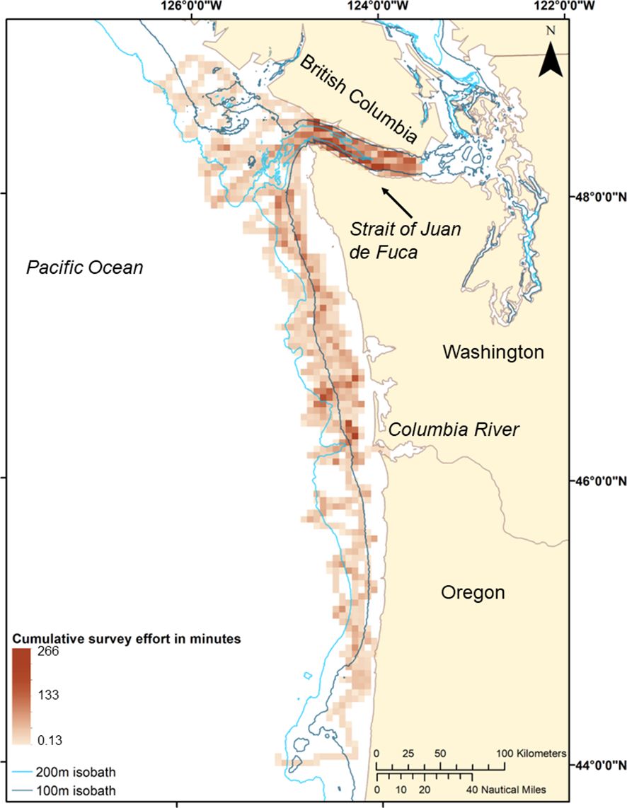
Figure 1 Combined daytime (0700-1800) survey effort, indicating minutes of effort per five square kilometers from four years of surveys (2006, 2008, 2009, and 2012) in winter (February, March, and/or early April). Darker 5-km bins indicate more time spent in this area. Cumulative survey effort in minutes was calculated from water temperature and salinity measurements that were collected every two seconds (2008, 2009, and 2012) to 15 seconds (2006).

Seabird surveys

Two trained observers conducted seabird distribution surveys during daylight hours (~0700-1800 local time) whenever the ship was travelling at speeds of ≥ ~2.5 m·s^-1 (5 knots). A primary observer counted and identified all birds detected within a strip transect extending 300 m out from the front of the ship in a 90-degree arc (Heinemann, 1981; Tasker et al., 1984). The general behavior of seabirds was recorded as either sitting on the water, actively feeding, engaging in directional flight (with flight direction recorded), engaging in non-directional flight, or following the ship. Observers used 8x42 binoculars and the unaided eye to detect and identify birds within the survey strip. Observers visually classified a seabird as a hybrid if it exhibited visual characteristics intermediate between two species. For example, for the western/glaucous-winged hybrid gull (Larus occidentalis x glaucescens), non-intermediate observations were classified as either glaucous-winged gull (Larus glaucescens) or western gull (Larus occidentalis). In fair weather, surveys were conducted from the flying bridge 12.6 m above the waterline; in conditions where rain exceeded a light drizzle, surveys were conducted from a sheltered bridge wing on the leeward (downwind) side of the ship 10.3 m above the waterline. The secondary observer assisted with bird identification and recorded all sightings into a laptop computer running the “SeeBird” data acquisition program v 2.3.0 (Southwest Fisheries Science Center [SWFSC], La Jolla, CA). This program allows each sighting record to include date, time, and latitude/longitude received from a NMEA 0183 global positioning antenna.

During survey periods, in situ water temperature (°C) and salinity (PSU) were recorded from the ship’s flow-through system, which has an intake at 3 m depth and used a Seabird Electronics SBE-19 conductivity-temperature-depth (CTD) instrument. Water temperature and salinity data were collected every two seconds (2008, 2009, and 2012) to 15 seconds (2006).

Marine mammal surveys

Three trained observers conducted marine mammal distribution and abundance surveys simultaneously with the seabird surveys using modified line-transect methods while the ship was travelling at speeds of 4.6–5.1 m·s^-1 (9–10 knots; Buckland et al., 1993). Observers recorded marine mammal sightings during daylight hours (~0700 to 1800). While this survey used Passive Acoustic Monitoring (PAM) to record mammal sounds with underwater hydrophones (Hanson et al., 2010) and recordings assisted with location of whales, only visual sightings with confirmed species identification were used in this analysis. In this study area, three ecotypes of killer whales coexist: offshore, transient, and resident killer whales (Bigg et al., 1990; Ford and Ellis, 1998; National Marine Fisheries Service, 2008). Ecotype separation includes known ecological, behavioral, and genetic differences, which are thought to be driven primarily by differences in diet and foraging behavior (Hoelzel and Dover, 1991; Ford et al., 2000). When possible, trained observers visually identified killer whales to ecotype (e.g. resident or transient) and population (e.g. Northern Resident or Southern Resident). For killer whales in this study, we observed only two ecotypes, one population of the mammal-eating, more cosmopolitan, transient ecotype; and two populations of the fish-eating, coastal resident ecotype: the Northern Resident killer whale (NRKW) and the endangered Southern Resident killer whale (SRKW).

Observers searched with 25x150 pedestal-mounted binoculars (“Big Eyes”), 7x50 hand-held binoculars, and the unaided eye. Two of the three observers scanned from 10 degrees across the ship’s path (i.e. trackline) to 90 degrees abeam with the 25x150 binoculars. An azimuth ring integrated with the 25x150 binocular mount allowed observers to report the sighting angle for each sighting. The third observer was positioned in the middle of the two other observers and scanned the area in front of the ship using 7x50 binoculars and the unaided eye. This observer also entered data (see below).

If the weather exceeded a sea state of Beaufort 4 (≥1.2–2.4 m waves and 17–21 knot (31.5–39 km/hr) winds) or rain/fog was present, the 25x150 binoculars were not used and two observers maintained a watch using 7x50 binoculars and the unaided eye. In fair weather, surveys were conducted from the flying bridge (see description in paragraph above); in conditions where rain exceeded a light drizzle, surveys took place from the interior bridge. The computer program WinCruz GPS (R. Holland, NOAA Fisheries, Southwest Fisheries Science Center) linked to the ship’s navigation system was used to record sighting date, time, GPS position, species identification, and number of individuals as well as other data, such as weather and sea state (Hanson et al., 2009).

Data layer preparation

Assigning any given sighting of a bird or mammal to an associated habitat variable for that time and location required preparing geo-referenced data layers for sightings and habitat variables. The following five habitat variables were derived from a bathymetry layer (85-m resolution DEM obtained from National Geophysical Data Center, NOAA) in in ArcGIS 10.7.1: depth (m), seafloor slope (%), shortest distance from shore (km), and shortest distances from the 100 m and 200 m isobaths (km). Salinity and sea surface temperature from shipboard in-situ measurements [collected every two seconds (2008, 2009, and 2012) to 15 seconds (2006)] during surveys were also georeferenced in ArcGIS 10.7.1.

Because seabird sightings occurred every few minutes and the survey coverage varied year to year, we assigned seabird sightings and their associated counts from a given year into 1 x 1 km bins, as determined by conversion into a year-specific 1 x 1 km raster grid. We converted these counts into year-specific estimated density (individuals per square kilometer) by dividing the total count of seabirds in each bin with the area surveyed in each bin (e.g. 1 km x 0.3 km = 0.3 square kilometers). Finally, the raster was converted back to vector and the geographical center of each 1 km x 1 km bin was paired with the five bathymetry-based habitat variables. Next, in-situ salinity and sea-surface temperature (SST) were averaged for each survey into 1-km bins, and the raster values for both salinity and SST were paired with each 1-km species- and year-specific seabird bin. When completed, each species-specific seabird bin was therefore associated with year-specific average values from seven distinct habitat variables. We explored 1 km, 3 km, and 5 km bin sizes and chose to bin the seabird density and all the habitat variables into 1-km segments after finding that 1-km spatial resolution successfully captured the fine-scale salinity and temperature features known to form near the coast, especially at the mouth of the Columbia River (Zamon et al., 2014).

We used the geographic coordinates for individual marine mammal sightings each year to pair directly with habitat data. Marine mammal counts were treated slightly differently than bird counts because the average distance between mammal sightings was 4.4 km, thus we would have lost the ability to resolve important habitat features of interest binning at this larger spatial scale (e.g., fine-scale temperature, salinity, and bathymetric features). For each sighting of one or more mammals, exact salinity and SST were paired with each species-specific marine mammal sighting by time and survey geographic location (+/- one second) using the rolling join function in data.table package (Dowle and Srinivasan, 2022) in the program R (R Core Team, 2019). Next, each marine mammal sighting was paired in ArcGIS with each of the five habitat variables described above (depth (m), slope (%), distance from shore (km), and distances from 100 m and 200 m isobaths (km). When completed, each marine mammal sighting record was therefore associated with seven distinct habitat variables.

Statistical analysis

1. Habitat variable overlap analysis (canonical correspondence analysis).

We conducted a canonical correspondence analysis (CCA; ter Braak, 1986) with the Vegan package (Oksanen et al., 2019) in R to identify species-specific habitat variable associations as well as to identify overlap in these associations (e.g. community ordination) among seabird and marine mammal species separately. A CCA is a constrained ordination technique that combines multiple explanatory variables of various units into a single variable or axis. Overall, CCAs are often used in community ecology because they can relate a matrix of community data (e.g. species abundance) to multiple explanatory variables. One of the major benefits of a CCA over other clustering or ordination analyses is that it combines multiple regression and ordination to conduct further statistical analysis and explore the significance of relationships among a community matrix of seabird density or marine mammal counts (response variables) and the seven habitat parameters (explanatory variables). Another key advantage to this method over linear methods is that species usually have a unimodal response to habitat variables or an environmental optimum (e.g., Shelford, 1931; ter Braak and Verdonschot, 1995). Thus, a CCA analysis is most similar to multivariate Gaussian regression, but robust to skewed species distribution, multicollinearity in species (ter Braak, 1986) and environmental data (Palmer, 1993), and atypical sampling design (Palmer, 1993). Variables were not standardized in the CCA, standardizing or normalizing has no impact on canonical correlations. But, for graphic representation we used “scaling 2” in the Vegan package to create a correlation biplot rather than a distance biplot, as our focus was the relationship between the seabird or marine mammal community and the habitat variables, not the locations at which species were observed.

To assess the significance of the full CCA model and of the canonical axes, we used a type of non-parametric test, an ANOVA (analysis of variance)-like permutation test. This permutation test leaves the explanatory variables (i.e. the habitat variables) fixed and randomly permutes, or rearranges, the response variables hundreds of times (i.e., marine mammal abundance or seabird density). Next, the observed F-statistic (the ratio of between-group variance to within-group variance) is compared to the distribution of the permutated F-statistics. A p-value is calculated from the proportion of permutated F-statistics that are equal to or greater than the observed F-statistic. The null hypothesis of this test is similar to a traditional ANOVA, that is, the association between the response and explanatory variables is the same as random chance, or more simply, that there is no association between the response and explanatory variables.

Despite small sample size, we conducted analyses on killer whales by ecotype rather than combining all ecotypes at the species level, because combining killer whale ecotypes at a species level would likely mask real differences in niche and habitat use in our CCA analysis for marine mammals.

2. Spatial habitat overlap analysis

To examine spatial distribution overlap among species, we plotted density and location (seabirds) or sighting counts (mammals) and location on maps of the survey area. For each of the seabird species and marine mammal species with more than or equal to 10 bins or sightings, we used the Directional Distribution (standard deviation ellipse) tool in ArcGIS 10.7.1. We did not calculate core winter habitat ellipses for any species with a sample size of less than 10 bins or sightings, with the exception of all killer whale ecotype sightings as they are of conservation concern, especially the Southern Resident killer whale population which is considered engaged under the Endangered Species Act of the United States and the Committee on the Status of Endangered Wildlife in Canada (COSEWIC). Moreover, the Northern Resident killer whale population is considered threatened by (COSEWIC) in Canada. These ellipses represent one standard deviation (~68%) of spatial distribution weighted by density for seabirds and counts for marine mammals. Similar to kernel density, we used these ellipses to represent “core winter habitat” within the area surveyed (i.e. core winter habitat ellipses).

Core winter habitat ellipses for seabird species with similar foraging modes were grouped onto the same map, resulting in four maps: surface-feeding procellariforms (dominated by black-footed albatross), surface-feeding larids (dominated by black-legged kittiwake), planktivorous divers (dominated by Cassin’s auklet), and piscivorous divers (dominated by common murre; Table 1). Similarly, for visualization purposes, we separated marine mammals into two foraging modes, large baleen whales (dominated by gray whales) and piscivorous toothed whales (dominated by Dall’s porpoise) on separate maps.

Table 1

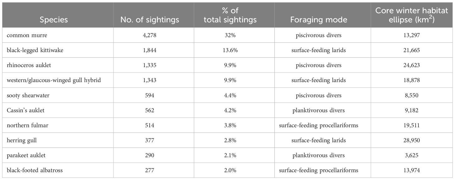
Table 1 Species name, number of sightings, percent of total sightings of the ten most commonly sighted seabird species (all bird species observed are listed in Supplementary Table 1) in the winter (February, March, and/or early April) of 2006, 2008, 2009, and 2012 in the northern California Current, foraging mode, and core winter habitat ellipses in km² calculated as 68% directional distribution weighted by density.

Once core winter habitat ellipses were defined, we used the Intersect tool in ArcGIS to calculate the area of overlap in km² between each pair of seabird or marine mammal species. For ease of interpretation, we categorized the proportion of overlap by qualitative categories (low ≤0.3 overlap, medium 0.31–0.59, and high ≥ 0.6).

Results

Species observed

Over the four years of surveys, 49 seabird species and ten marine mammal species were observed. The ten most frequently sighted bird species were common murre (32%), black-legged kittiwake (Rissa tridactyla, 13.6%), western/glaucous-winged hybrid gull (9.9%), rhinoceros auklet (Cerorhinca monocerata, 9.9%), sooty shearwater (Ardenna grisea, 4.4%), Cassin’s auklet (Ptychoramphus aleuticus, 4.2%), northern fulmar (Fulmarus glacialis, 3.8%), herring gull (Larus argentatus, 2.8%), parakeet auklet (Aethia psittacula, 2.1%), and black-footed albatross (Phoebastria nigripes, 2.0%), respectively (Table 1; Supplementary Table 1). These ten species made up 84% of total bird sightings (n = 11,414 sightings). The mean group size per sighting (μ) of the top ten seabird species was highest for common murres (μ = 5.5, range: 1–1,200) and lowest for herring gull and black-footed albatross (μ=1.1, range: 1–5 and 1–10, respectively) (Supplementary Table 1).

Marine mammals were sighted far less often than seabirds with only 243 total sightings. The top five marine mammals accounted for 82% of all sightings (Table 2; Supplementary Table 1) and the top three species of marine mammal species had similar frequencies of sighting, gray whale (Eschrichtius robustus, 24%), harbor porpoise (Phocoena phocoena, 23%), Dall’s porpoise (Phocoenoides dalli, 22%). The next two most frequently sighted species were the Pacific white-sided dolphins (Lagenorhynchus obliquidens) and killer whales; these two species had the largest average group size (μ = 13.3, range = 5–35; and μ = 12.6, range = 3–42). By contrast, only individual minke (Balaenoptera acutorostrata) and sperm (Physeter macrocephalus) whales were observed, and just one to two sightings of each species were made over the four survey years (Supplementary Table 1). Resident killer whales (NRKW and SRKW combined) met the minimum number of sightings to be included in the CCA and directional distribution overlap, core winter habitat ellipse analysis (i.e. ≥ 10).

Table 2

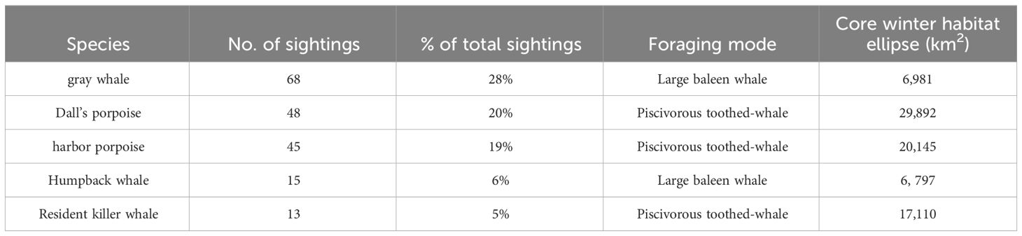
Table 2 Species common name, number of sightings, percent of total sightings of the five commonly sighted marine mammals (with greater than 10 sightings; see Supplementary Table 1) in the winter (February, March, and/or early April) of 2006, 2008, 2009, and 2012 in the northern California Current, foraging mode, and core winter habitat ellipses in km² calculated as 68% directional distribution weighted by abundance.

Seabirds

The matrix of seabird community density of the top 10 most frequently sighted species was significantly associated with all habitat variables (999 permutations, p = 0.001), but the variance explained by the habitat variables was low (R² = 0.11). A step-wise forward selection (199 permutations) found that the model that included all seven habitat variables was the most parsimonious model. Seabird density for the top ten most commonly sighted species was significantly associated with the first five axes from the CCA (CCA1–5, p ≤0.002) and most associated with distance from coast (component loading: -0.85) and sea surface temperature (SST; 0.62) along CCA1 (x-axis; 6.8% of total variance). Along CCA2 (y-axis; 2.3% of total variance), seabird density was most associated with distance from 100 m isobath (0.53) and depth (-0.50) (Figure 2).

Figure 2

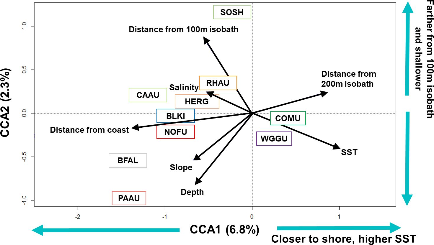
Figure 2 Ordination biplot for the canonical correspondence analysis of the top ten most commonly sighted seabird species during the winter/downwelling season (February, March, and/or early April) of 2006, 2008, 2009, and 2012 in the northern California Current. Species plotted on the first two axes (CCA1, CCA2, % variance explained for each axis is provided). Black arrows show the relative importance of each of the habitat variables (length of arrow) and correlation (i.e. angle) with axes (i.e. habitat variables). Four letter species codes are: BFAL, black-footed albatross; BLKI, black-legged kittiwake; CAAU, Cassin’s auklet; COMU, common murre; HERG, herring gull; NOFU, northern fulmar; PAAU, parakeet auklet; RHAU, rhinoceros auklet; SOSH, sooty shearwater; and WGGU, western/glaucous-winged gull hybrid.

Based on the seven habitat variables examined, three species [black-footed albatross (BFAL), sooty shearwater (SOSH), and parakeet auklet (PAAU)] were located farther from other seabirds in the CCA ordination bi-plot (Figure 2). Black-footed albatross and parakeet auklets observed in these surveys were found in deeper water, and farther from the coast and the 100 m isobath in comparison to all other seabird species; with parakeet auklets found in the deepest water and closest to the 100 m isobath. Sooty shearwaters were found in the shallowest water and farthest from the 100 m isobath. The other seven seabird species fell into two clusters: western/glaucous-winged hybrid gulls (WGGU) and common murres (COMU) were found in warmer waters and closest to shore of all the seabirds, herring gulls (HERG), rhinoceros auklets (RHAU), and black-legged kittiwakes (BLKI) were found farther from shore in areas of moderate depth and temperature (Figure 2).

When examining the spatial distribution of seabird density within a foraging mode across all four years of available data, piscivorous divers (common murre, sooty shearwater, and rhinoceros auklet), the mean center of common murre density was found 119–150 km farther south from the centers for rhinoceros auklet and sooty shearwater, respectively, which were closer together (30 km; Figure 3A). Moreover, common murres had the largest core winter habitat ellipse in comparison to the other piscivorous divers (13,297 km²) and shared close to half of their core habitat with rhinoceros auklets and sooty shearwaters (51% and 42%, respectively). Rhinoceros auklet shared only approximately a third of their core habitat with common murres and sooty shearwaters (28% and 35%, respectively), and sooty shearwaters shared most of their core habitat with murres and rhinoceros auklets (65% and 100%, respectively; Table 3).

Figure 3

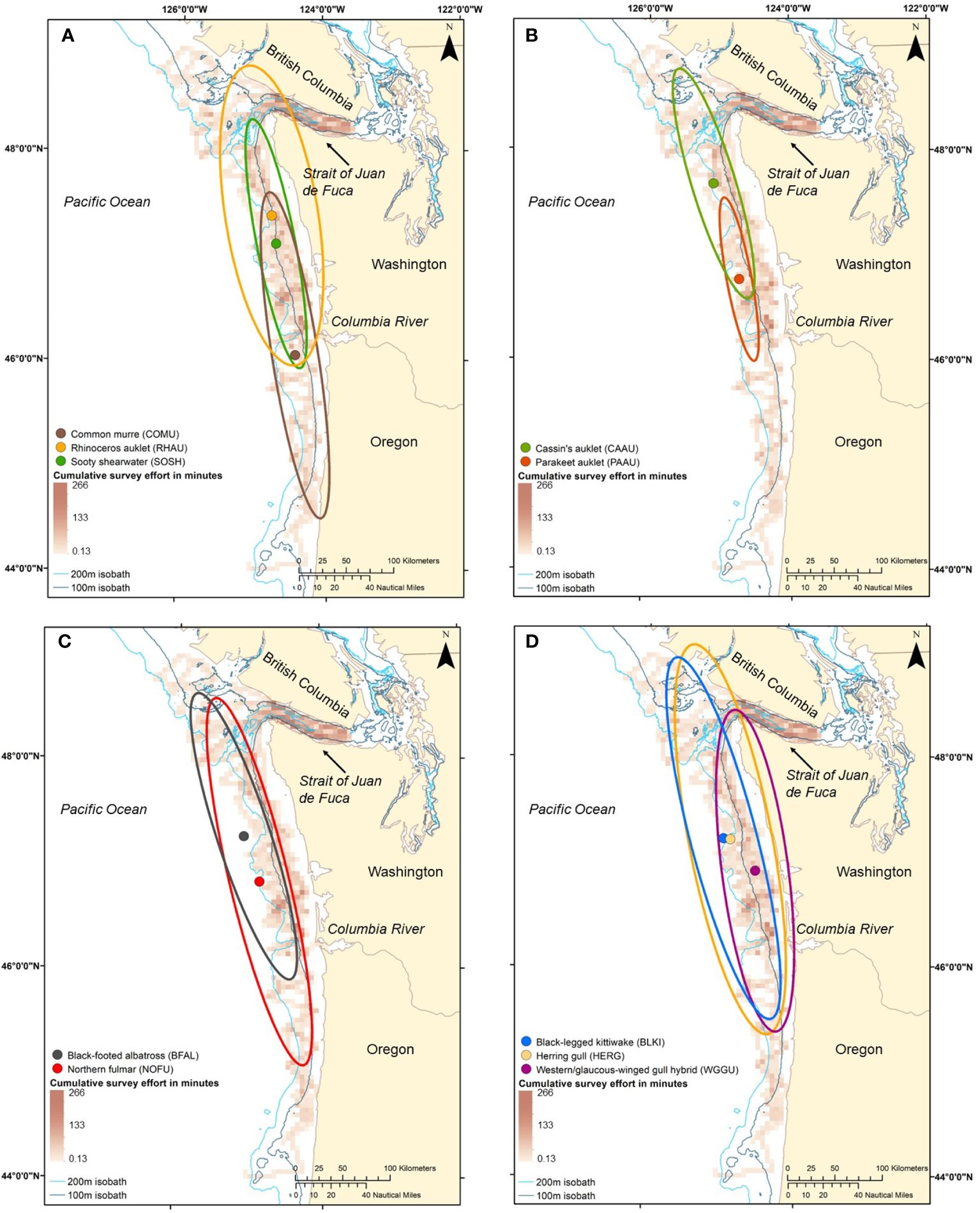
Figure 3 (A–D) Mean center and spatial overlap of the core winter habitat ellipses (i.e. 68% directional distribution ellipses) of all four foraging modes of seabirds, piscivorous divers [(A); common murre, sooty shearwater, and rhinoceros auklet], planktivorous divers [(B); Cassin’s auklet and parakeet auklet], surface-feeding procellariforms [(C); black-footed albatross and northern fulmar], and surface-feeding larids [(D); black-legged kittiwake, herring gull, and western/glaucous-winged gull hybrid] weighted by density of individuals per 1-km. Red gradient raster shows combined daytime (0700–1800) survey effort, minutes of effort per 5 square kilometers from winter/downwelling surveys. Note that portions of any ellipse that occur on land do not indicate seabirds normally occur on land; the coastline serves as the true habitat boundary.

Table 3

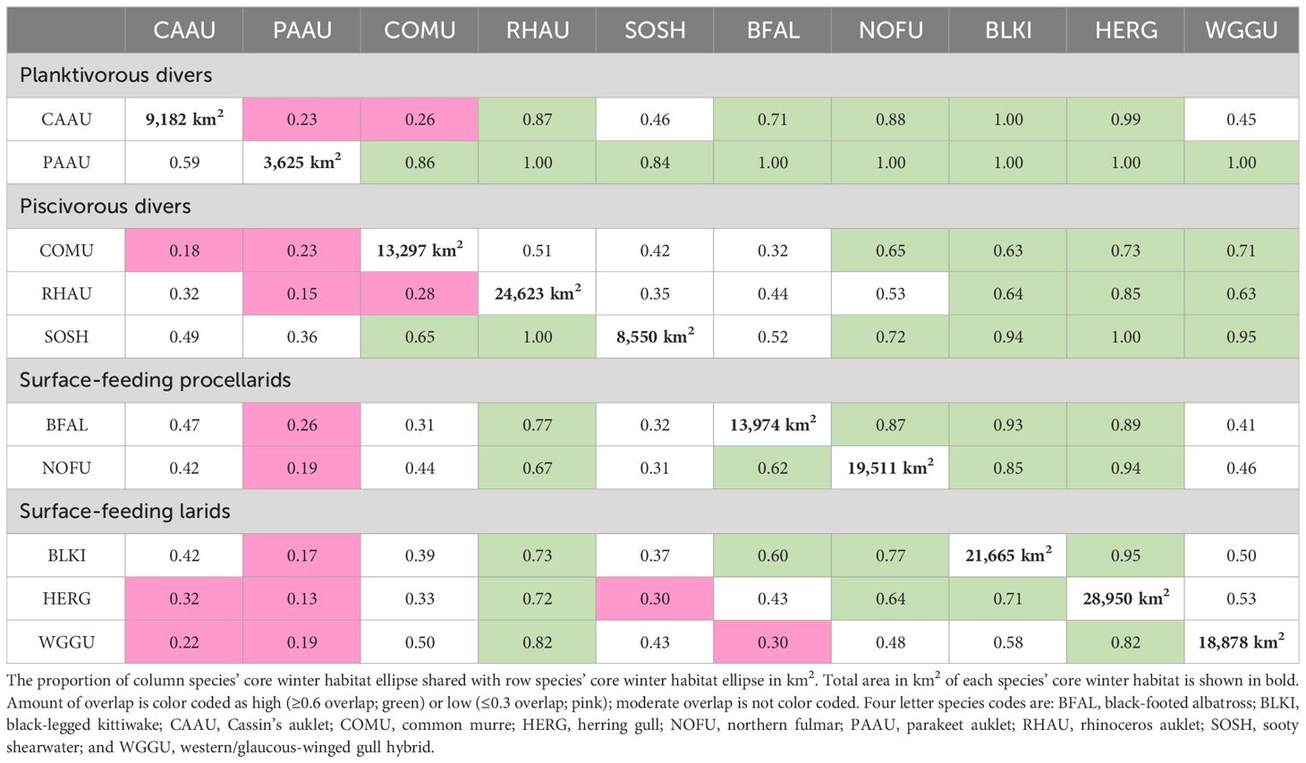
Table 3 Row and column headings are each of the seabird species included in this analysis.

For the planktivorous alcids (Cassin’s auklet and parakeet auklet) showed some separation by latitude, with the mean center of parakeet auklet density found 105 km south of that for Cassin’s auklet (Figure 3B). In addition, the Cassin’s auklet core winter habitat was 2.5 times larger than the core habitat of parakeet auklet (9,182 and 3,625 km² respectively). Only 23% of Cassin’s auklet core habitat overlapped with that of parakeet auklets, and 59% of parakeet auklet’s core habitat overlapped with that of Cassin’s auklet (Table 3).

Surface-feeding procellariforms (northern fulmar and black footed albatross) had overall high overlap in core habitat, with the black-footed albatross sharing 87% of their core habitat with northern fulmars and northern fulmars sharing 62% of their core habitat with black-footed albatross (Figure 3C; Table 3). The mean center of northern fulmar density was found 51 km south of black-footed albatross density, but the Northern Fulmar core winter habitat ellipse extended farther south into Oregon, USA.

The three surface-feeding larids (black-legged kittiwake, herring gull, and western/glaucous-winged gull hybrid) had the largest core winter habitat ellipses in comparison to all other seabird species (Table 1; 18,878–28,950 km²). The mean center of density for herring gulls and black-legged kittiwakes were extremely close at this scale (7.3 km; Figure 3D); however, the mean center of western/glaucous-winged gull hybrid density was found 42 and 48 km southeast from herring gulls and black-legged kittiwakes, respectively. Herring gulls shared a high proportion of their core habitat with black-legged kittiwakes (71%), and a moderate proportion with western/glaucous-winged gull hybrid (53%). However, western/glaucous-winged gull hybrids shared a high proportion of core winter habitat with herring gulls (82%) and a moderate proportion with black-legged kittiwakes (58%). Black-legged kittiwakes shared a high proportion of core habitat with herring gull (95%) and a moderate proportion with western/glaucous-winged gull hybrid (50%).

Marine mammals

The matrix of marine mammal community abundance was significantly associated with all habitat variables (999 permutations, p = 0.001), but explained variance by the model was low (R² = 0.12). A step-wise forward selection found that a model with only temperature, depth, salinity, and distance from coast was the most parsimonious; however, this reduced model did not strengthen the variance explained (R² = 0.10). Marine mammal abundance was significantly associated with CCA1 (5.2% of total variance, p = 0.003) and CCA2 (3.9% of total variance, p = 0.006). CCA1 was most associated with SST (-0.83) and CCA2 with salinity (0.80) and depth (0.54) (Figure 4).

Figure 4

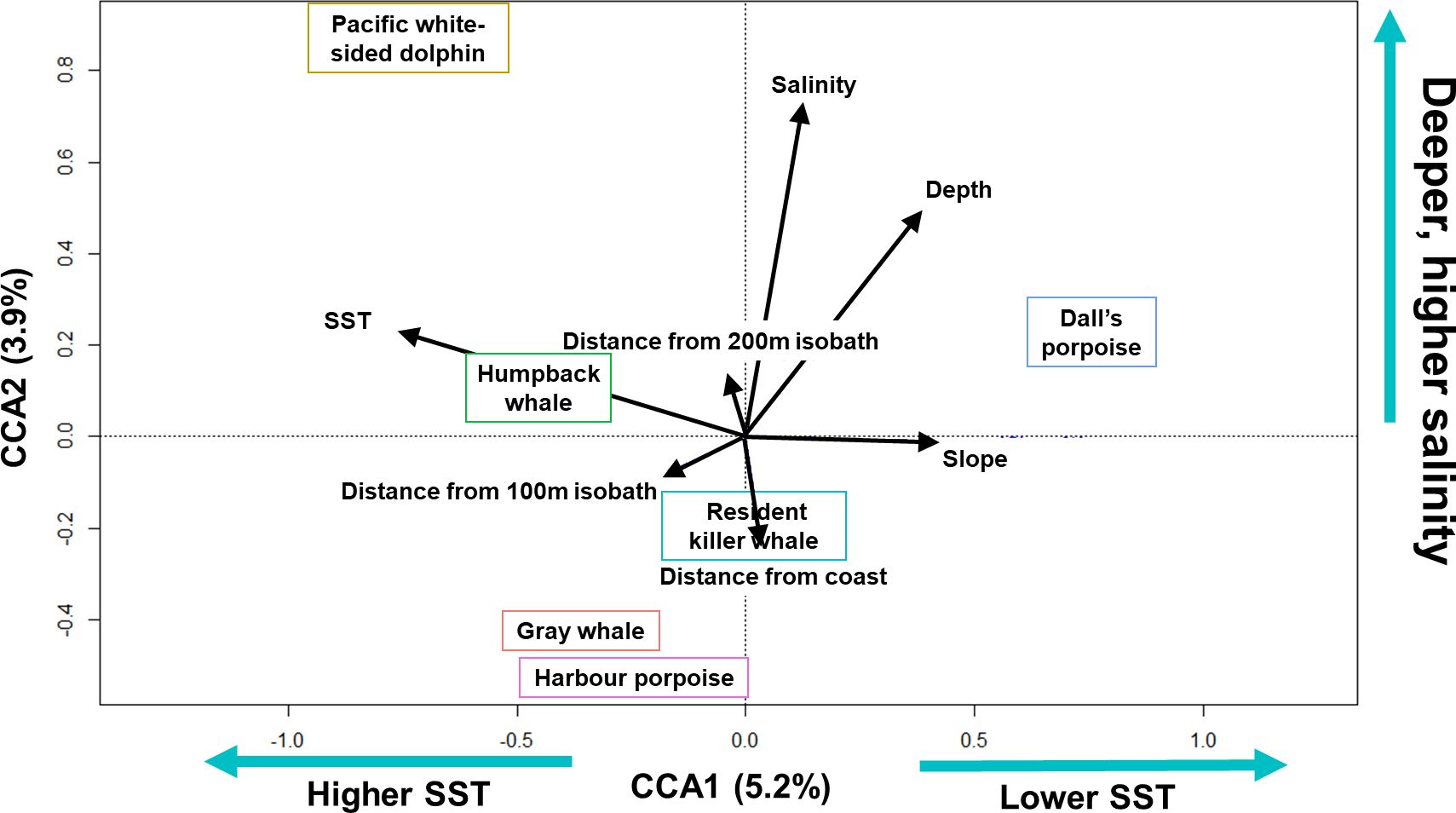
Figure 4 Ordination biplot for the canonical correspondence analysis of the six most commonly sighted marine mammal species during the winter/downwelling seasons (February, March, and/or early April) of 2006, 2008, 2009, and 2012 in the northern California Current. Species plotted on the first two axes (CCA1, CCA2, % variance explained for each axis is provided). Black arrows show the relative importance of each of the habitat variables (length of arrow) and correlation (i.e. angle) with axes (i.e. habitat variables). Resident killer whale category combines sightings of northern and southern resident killer whales.

Three species (humpback whales, Pacific white-sided dolphins, and Dall’s porpoise) did not cluster with other marine mammal species in habitat associations (Figure 4). Compared to other species, Pacific white-sided dolphins were associated with deeper, higher salinity areas, Dall’s porpoise tended to be in colder water, while humpback whales tended to be in waters of moderate temperature and moderate depth.

In contrast, piscivorous resident killer whales were associated with moderate salinity and temperature (Figure 4), but more associated with distance from the coast (i.e. the y-axis) in comparison to Pacific white-sided dolphins, humpback whales, and Dall’s porpoise. Despite their ecological differences, gray whales and harbor porpoises were close together on the ordination plot (Figure 4), indicating associations for both species with shallower water with lower salinity and moderate sea surface temperature.

When examining the spatial distribution of marine mammals with similar foraging modes, the baleen whales showed some spatial segregation by latitude; the mean center of humpback whale abundance was 11 km southeast of that for gray whales (Figure 5A). There was also low spatial overlap in core winter habitat for gray and humpback whales, and neither whale shared more than 22% of their core habitat with the other species (Table 4).

Figure 5

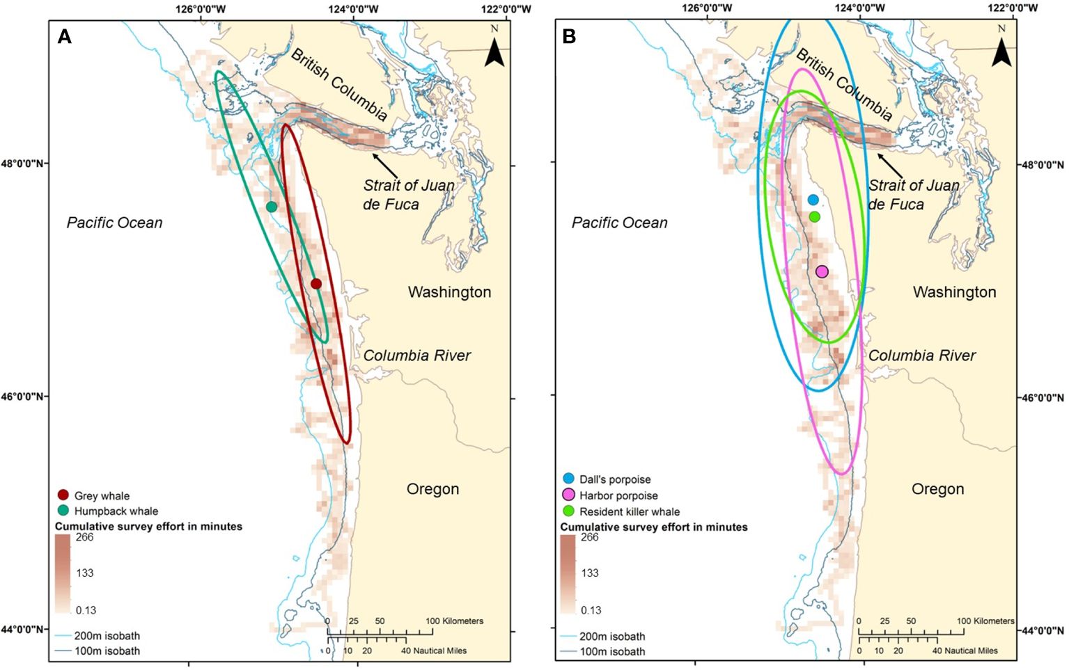
Figure 5 (A, B). Mean center and spatial overlap of the core winter habitat ellipses (i.e. 68% directional distribution ellipses) of two foraging modes of marine mammals, baleen whales (A) gray whale and humpback whale] and toothed whales (B) Dall’s porpoise, harbor porpoise, and resident killer whale (northern and southern resident sightings combined], weighted by abundance (number of individuals). Red gradient raster shows combined daytime (0700–1800) survey effort, minutes of effort per 5 square kilometers from four years of surveys in the winter/downwelling seasons (February, March, and/or early April) of 2006, 2008, 2009, and 2012. Note that portions of any ellipse that occur on land do not indicate the presence of marine mammals on land; the coastline serves as the true habitat boundary.

Table 4

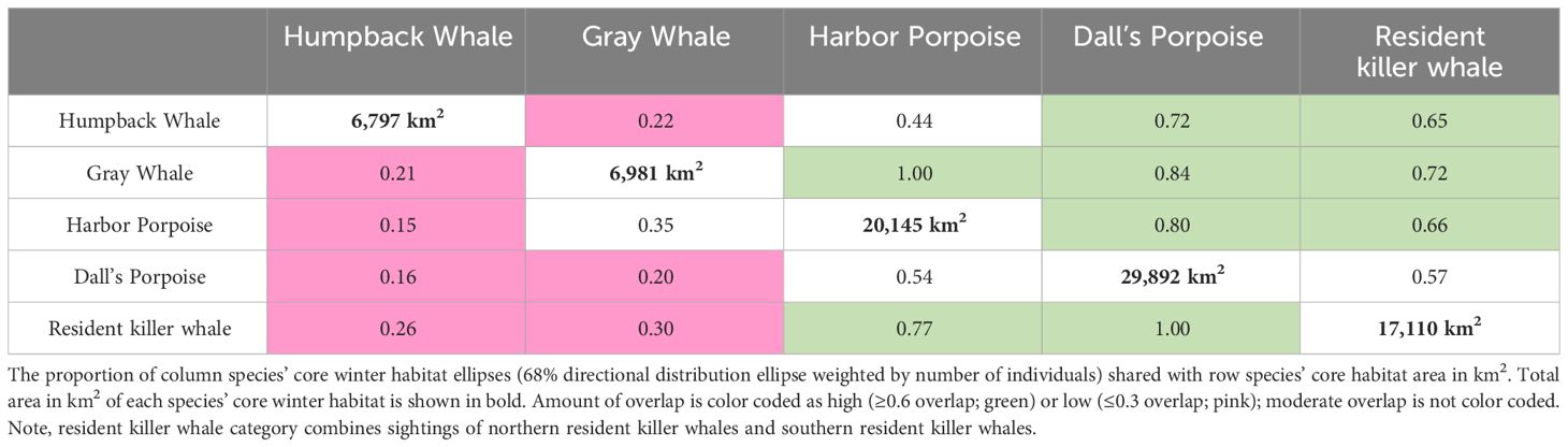
Table 4 Row and column headings are each of the marine mammal species included in this analysis.

For piscivorous toothed whales, the mean center of abundance for harbor porpoises was 69 km south of that of Dall’s porpoise while the mean center of abundance for resident killer whales was 16 km south of that of Dall’s porpoise. However, the two porpoise species had moderate to high spatial overlap of core winter habitat with harbor porpoises sharing 80% of their habitat with Dall’s porpoises and Dall’s porpoises sharing 54% of their core winter habitat with harbor porpoises (Figure 5B). Resident killer whales also had high overlap in core winter habitat with both Dall’s porpoise and harbor porpoises (77–100%) and lower overlap with humpback whales and gray whales (26–30%, Table 4). In general, baleen whales had a narrower core winter habitat ellipse across the continental shelf and, thus, a smaller area of core winter habitat (6,797–6,981 km²) in comparison to piscivorous toothed whales (17,110–29,892 km²; Table 4).

Overall, the majority of all killer whale sightings were along the Washington shelf despite considerable survey effort along the Oregon shelf (Figure 6). Only one killer whale sighting (transient ecotype; 15 individuals) was found south of Columbia River mouth and no killer whales were observed north of the Strait of Juan de Fuca, although there was lower spatial and temporal survey effort north of the Strait of Juan de Fuca (Figure 1). The resident ecotype, the Northern Resident Killer Whale population, were found along the Washington coast between the entrance of the Strait of Juan de Fuca and just north of the mouth of the Columbia River. Southern Resident Killer Whale sightings were more spatially aggregated and were mostly found inside the Strait of Juan de Fuca or at the mouth of the Columbia River. Transient ecotype killer whales were evenly distributed along the Washington and Oregon coast from the northern tip of Washington to the mouth of the Columbia River.

Figure 6

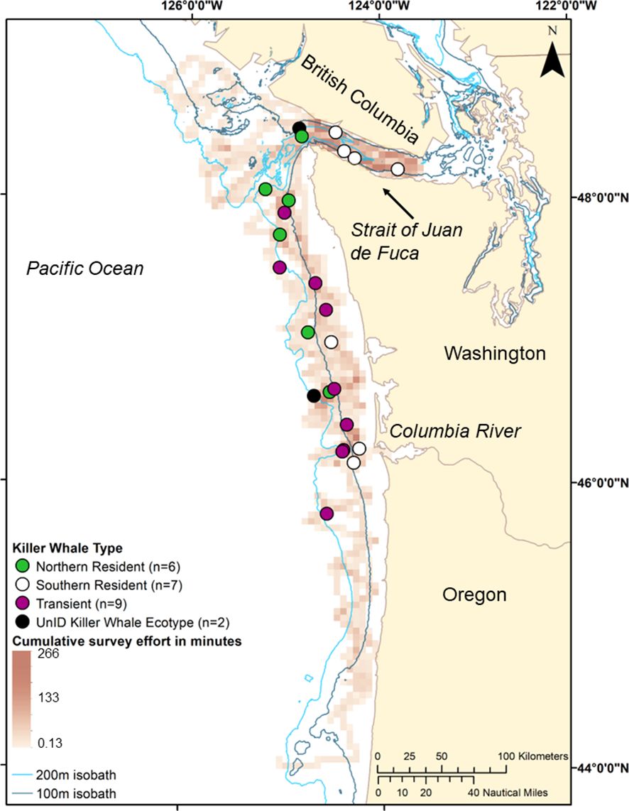
Figure 6 Spatial distribution of killer whale ecotypes observed in the winter/downwelling seasons (February, March, and/or early April) of 2006, 2008, 2009, and 2012 in the northern California Current. Red gradient raster shows combined daytime (0700– 1800) survey effort, minutes of effort per 5 square kilometers from four years of surveys in the winter/downwelling seasons (February, March, and/or early April) of 2006, 2008, 2009, and 2012.

Discussion

Despite the generally low productivity of the winter downwelling season compared to the summer upwelling season, we observed 49 species of seabirds and ten species of whales inhabiting the northern CCE during the winter months. From these four years of winter surveys, we saw evidence for significant, but weak, differences in winter habitat use. That is, niche separation by species via CCA analysis within four seabird foraging mode types and two whale foraging mode types. We used a CCA to investigate niche partitioning and the results showed differentiation among species in habitat variable associations (i.e. segregation), suggesting some degree of niche partitioning of habitat; that is, lower overlap in habitat use within a foraging mode type when primary productivity is low during the winter downwelling season. Our CCA results also indicated that in-situ sea surface temperature was the strongest correlate of marine mammal abundance and the second strongest correlate of seabird density during the winter.

While overall CCA statistical explanatory power was low, the strongest habitat associations found in this study were similar to those found in previous CCE studies during summer for seabirds [i.e., Ainley et al., 2005: salinity; Oedekoven et al., 2001: sea surface temperature (SST)] and whales (i.e. Tynan et al., 2005: SST, depth, and salinity). During summer, some of the strongest associations for seabirds in previous CCE studies were with seasonally-persistent upwelling fronts (Hoefer, 2000; Oedekoven et al., 2001), especially for species such as piscivorous divers, planktivorous divers, and surface-feeding procellarids (Ainley et al., 2005). However, the surface structures associated with these fronts are absent in the winter season, due to the reversal in surface winds that results in downwelling conditions and increased surface wind-mixing (Hickey, 1979; Huyer et al., 2007). Some species-specific habitat associations found in summer seem to persist even during winter downwelling, such as Cassin’s auklets being found in cooler water during both seasons, potentially because their preferred prey, the krill species Thysanoessa spinifera, is associated with cooler, nutrient-rich water (Oedekoven et al., 2001). Additionally, some important winter habitat variables identified by a recent large-scale, seasonally-averaged CCE seabird distribution model were in agreement with our CCA results for species such as common murre (i.e. SST) and black-footed albatross (i.e. distance to coast) (Leirness et al., 2021). However, the most influential variables for these species-specific models in the winter were habitat features that were not measured in this study such as chlorophyll-a concentration and turbidity (Leirness et al., 2021).

Although the CCA explained a fairly low proportion of the total variation in seabirds or marine mammals, this is not unusual for the CCE. The proportion of total variance explained (e.g. explained deviance) by models using physical and biological variables can be low in the CCE even during the highly productive summer upwelling season (e.g. Ainley et al., 2005: average 25% explanation for observed seabird species), but explained deviance can also be much higher or lower if models are single species-specific for seabirds (e.g., Ainley et al., 2005: 8–44%) and whales (Tynan et al., 2005: 26–95%; Forney et al., 2015: 2–19%). Low explanatory power even within the high productivity of the summer upwelling season could be due to a variety of reasons, including a lack of direct measurements of one important variable, prey. We also acknowledge that our relatively low sightings for whales (242 sightings over four years), leads our statistical power to resolve habitat associations to be lower than other modeling efforts with larger sample sizes (e.g., Tynan et al., 2005: 223 total sightings in spring and 298 in summer in a single year; Forney et al., 2012: >17,000 sightings of cetacean groups, 20 years of data).

Another possible explanation for the weak correlations in the CCA between seabird density or marine mammal abundance and the habitat features we measured is the presence of migrating or non-resident species that may not be using this area primarily for foraging during the winter. For example, some proportion of the gray whale population is thought to be migrating north between breeding grounds in Mexico and summer foraging grounds in Alaska (Sato and Wiles, 2021a). Additionally, the distribution of some species in the CCE, such as the black-footed albatross and northern fulmar, may be affected not only by specific prey-habitat cues but also by fishing vessel distribution, given that some seabird species are attracted to fishing discards or bait as a source of food (Jannot et al., 2021). However, fishing activity was not a factor measured in this study.

Spatial overlap among species was higher than expected, indicating low partitioning, or niche separation, in space during winter in the CCE. There was also asymmetric spatial overlap in our study for the planktivorous parakeet auklet, which shared 86% of its core winter habitat in this region with the common murre; but the common murre, an adaptive generalist in the winter (Ainley et al., 1996), only shared 23% of its core winter habitat with the parakeet auklet. In the summer, diet overlap between the common murre and parakeet auklet is thought to be low, with common murres focusing more on higher trophic level prey such as fishes and parakeet auklets focusing on lower trophic level prey such as zooplankton and invertebrates (Hobson et al., 1994). Winter studies, although few, show that common murres continue to primarily consume fishes during the winter (Baltz and Morejohn, 1977), but this species is also extremely adaptable and can increase diving capacity to reach deeper prey (Burke and Montevecchi, 2009) and even switch its diet to lower trophic levels, such as euphausiids, based on prey availability (Ainley et al., 1996). In this study, murres were more abundant, occupied a much larger spatial area in the northern CCE, had a mean center of distribution close to parakeet auklets, and thus, potentially had greater flexibility in foraging behavior than parakeet auklets. This asymmetrical overlap implies that in the case of ecosystem perturbations that could increase inter- and intra-specific competition such as marine heatwaves (e.g. Piatt et al., 2020), one species can be more negatively affected than the other.

In contrast to observed asymmetric spatial overlap, we observed evidence for symmetrical niche partitioning in space between the two baleen whale species, gray whales and humpback whales. Each of these species shared only 21–22% of its core winter habitat with each other. Although they are both baleen whales, they have very different diets and foraging modes; humpback whales are filter feeders that can take advantage of a variety of prey such as krill and fishes, by foraging at the surface and to depths of up to 360 m (Palacios et al., 2020). By contrast, gray whales filter feed on benthic prey and forage coastally at depths from 50 m to as shallow as 10 m (Nelson et al., 2008). Despite differences, there is some degree of known diet overlap between these two species in that they will both consume krill (Sato and Wiles, 2021a, 2021b).

Historically, it has been understood that gray and humpback whales migrate during the winter and early spring months and transit through the CCE with limited feeding during migration (Swartz, 2014; Sato and Wiles, 2021b). However, both species have been commonly detected in the CCE via passive acoustic instrumentation throughout the winter and spring (Emmons et al., 2021; Rice et al., 2021), with higher numbers of acoustic detections during the winter along the northern domain (Širović et al., 2011; Emmons et al., 2021). Further, hundreds of gray whales (e.g. Pacific Coast Feeding Group) have been known to forage in the northern CCE as well into the fall (September–December, Lagerquist et al., 2019), which is the beginning of the CCE downwelling season. At least one gray whale individual has been observed overwintering in this area (Lagerquist et al., 2019), and gray whales have been sighted nearshore at the Columbia River year-round (Zamon, unpublished data). In this study, gray whales were the most frequently sighted whale (28% percent of all sightings), although we were unable to distinguish between migrating gray whales and resident gray whales during these surveys. Humpback whales and gray whales have different foraging modes and migration strategies, however, because their ranges overlap, the impacts of climate change in winter are likely to affect both species in a similar way.

As little is known about winter habitat use in this area for killer whales, especially resident killer whales, the observations from this study, albeit few, are important to note. There were enough resident killer whale observations to include in both the CCA and spatial overlap analysis although we did have to combine Northern and Southern residents for the analysis, which may mask any population-specific habitat associations. Spatial overlap was high between resident killer whales and the other toothed whale species (77–100%); however, resident killer whales have a much more specialized diet that includes a large portion of Chinook salmon year-round (Hanson et al., 2021) and, thus, may not be responding to habitat features similar to other toothed whales during the winter. Instead, resident killer whales may be responding to the timing of early spring Chinook salmon runs returning to rivers from California to Washington (Zamon et al., 2007). Indeed, we saw Southern Resident Killer Whales at freshwater output areas during our surveys (Figure 6; i.e., Columbia River and Strait of Juan de Fuca). Although still dominated by Chinook salmon, recent diet studies have found a higher diversity of prey in Southern Resident killer whale diets in winter, which may be due to decreasing numbers of endangered Chinook salmon populations (Hanson et al., 2021).

We found higher spatial overlap in core winter habitat ellipses between tubenose and gull species with lower energetic cost for flight and better gliding capabilities species (i.e. surface-feeding procellarids and larids, see Table 1; Elliot et al., 2013) in comparison to pursuit diving species like alcids (e.g., common murre and Cassin’s auklet) and thus overall weak evidence of niche partitioning in space for these foraging types. This is consistent with what Baltz and Morejohn (1977) reported, they observed these species in large mixed-species foraging groups with high dietary overlap (via stomach contents) in winter in the CCE. For these surface-feeding seabird species, visual cues that result in social attraction among foraging predators (Haney et al., 1992) may provide mutually beneficial effects, especially at a time when prey may be less abundant or more difficult to detect (Veit and Harrison, 2017). In contrast, less mobile species such as piscivorous and planktivorous divers had lower overall spatial overlap and smaller overall core winter habitat. This has the potential to make them less resilient to perturbations which affect prey distribution, availability, or quality (Slatyer et al., 2013; Cooke et al., 2019). Therefore, based on the results of this study, we suspect that the five species of piscivorous and planktivorous divers observed in this study, especially the Alcidae species, would be most vulnerable to perturbations in this domain of the CCE. This increased vulnerability would result from a combination of lower mobility, a higher energetic cost of mobility (Pennycuick, 1987; Elliot et al., 2013), and lower food availability. Support for this idea was provided during a recent marine heatwave in the CCE (“the blob”) from 2014–2016 (Gentemann et al., 2017), which led to large-scale starvation events of marine species along the west coast of North America and disproportionately affected auklet species (Jones et al., 2018; Piatt et al., 2020).

Our study showed that SST is an important factor in species habitat associations during the downwelling season. Therefore, we expect temperature changes in winter SST to have broad effects on winter species distributions. For example, worldwide marine heatwaves have become more frequent and longer in duration over the last 100 years (Oliver et al., 2018), with the frequency of marine heatwaves doubling in the last 30 years (Frölicher et al., 2018). Marine heat waves cause temporary temperature increases of similar magnitude (Bond et al., 2015) as median increases in winter SST in the CCE predicted from climate models (from 1.1 to 3.1°C depending on the model (Iturbide et al., 2021)). In this respect, marine heat waves may serve as a kind of “dress rehearsal” for climate change effects on species distributions and food webs. Previous studies have shown that marine heatwaves can have long-lasting negative impacts on ecosystem function in the CCE, direct impacts on marine predators includes displacement and loss of core habitat area for seabirds and whales (Welch et al., 2023), reducing reproductive success in seabirds (Piatt et al., 2020) and whales (Cartwright et al., 2019), shifts in whale distributions that increase whale entanglement in fishing gear (Santora et al., 2020), and effects on food web processes such as competition via habitat compression (Piatt et al., 2020). Moreover, marine heatwave impacts on lower trophic levels and prey includes reducing krill size (Robertson and Bjorkstedt, 2020) and lipid content (Killeen et al., 2022), reducing biomass and shifting distribution of fishes (Cheung and Frölicher, 2020). We did see inter-annual variation in SST during our surveys (Supplementary Figures 1–4), but none of our surveys occurred during a heat wave, and differences in survey timing and spatial coverage meant we could not directly investigate inter-annual effects of temperature with only four years of data.

After these surveys took place, there has been an extended period of ocean warming (Gentemann et al., 2017; Jones et al., 2018; Piatt et al., 2020; Santora et al., 2020), and ocean temperature has remained above average in the southern domain of the California Current from 2013 to 2020 inclusive (Weber et al., 2021). Therefore, if it were possible to repeat these winter surveys, data from this study could provide important base information on the winter distribution of seabirds and marine mammals in the CCE prior to the marine heatwaves in 2014–2016 and higher than average sea surface temperatures in 2018–2020 (Weber et al., 2021). Additionally, developing knowledge of species-specific winter distribution and abundance can aid in calculating the impacts of past and future winter mortality events (e.g., Jones et al., 2018: Cassin’s auklet die-off during heatwave; Gulland et al., 2005: gray whale strandings; and Stepanuk et al., 2021: marine mammal vessel strikes).

We recommend that future surveys during the downwelling season include not only surveys of bird and mammal predators, but also surveys of intermediate trophic levels (i.e., plankton, krill, and forage fishes) and predator diet, as we still know very little about winter trophic interactions and winter oceanography in this region compared to the upwelling season. Survey methods could include both more traditional methods to sample prey organisms or diet (e.g. nets, hydroacoustic, and scat or stomach contents) as well as isotopic, biochemical, or genomic techniques that can identify trophic links between consumers and producers (e.g. stable isotopes, lipid content, eDNA, DNA metabarcoding). For example, there are already-established techniques to map krill distributions in the CCE with hydroacoustics and compare them with predator distributions (Phillips et al., 2022; Kaplan et al., 2024). And while weather and sea state limitations make it difficult to conduct net sampling during this period, it may be possible to use eDNA from depth-stratified water samples to learn something about the distribution of prey species during downwelling periods (Shelton et al., 2022). Without sampling prey distribution, it is not possible to determine what factors might be ultimately responsible for the presence or absence of niche partitioning. For example, differences in “foraging arenas”, where prey are available to one type of predator but not to another (Ahrens et al., 2012) could explain differences between gray whale and humpback whale habitat ellipses. Establishing an understanding of predator-prey distributions and food web links during winter downwelling is critical because we currently have so little information on this topic for the northern CCE. Other work has shown that heatwave-driven shifts in prey quality and predator metabolism can lead to increased competition among marine predators with shared prey resources, which caused massive die-offs and breeding failure of the common murre in the CCE (Piatt et al., 2020).

Data availability statement

The original contributions presented in the study are included in the article and Supplementary Material. Further inquiries can be directed to the corresponding author.

Ethics statement

The animal study was approved by the NMFS permit office. The NMFS permit office reviewed all methods and protocols, and all work was conducted under NOAA Research Permits, numbers 16111 and 16163. The study was conducted in accordance with the local legislation and institutional requirements.

Author contributions

LB: Data curation, Investigation, Methodology, Project administration, Visualization, Writing – original draft, Writing – review & editing. JZ: Conceptualization, Data curation, Supervision, Writing – review & editing. GD: Conceptualization, Methodology, Supervision, Writing – review & editing. BH: Funding acquisition, Investigation, Project administration, Resources, Writing – review & editing. DN: Investigation, Project administration, Writing – review & editing. CE: Data curation, Investigation, Project administration, Writing – review & editing. MH: Investigation, Project administration, Resources, Writing – review & editing.

Funding

The author(s) declare financial support was received for the research, authorship, and/or publication of this article. The Ph.D. work of LB was funded by UofM. Funding for these at sea surveys was provided by the NMFS Northwest Fisheries Science Center. Oregon Wave Energy Trust provided additional funding for the 2012 survey.

Acknowledgments

This manuscript was greatly improved by comments from D. K. Hyrenbach, K. Jacobson, and L. Weitkamp and two reviewers. Enormous thanks to the intrepid and dedicated captains and crew of NOAA vessels McArthur II and Bell M. Shimada as well as all the hardworking marine bird and mammal observers including B. Phillips. Funding for these surveys was provided by the NMFS Northwest Fisheries Science Center. Enormous thanks to the intrepid and dedicated captains and crew of NOAA vessels McArthur II and Bell M. Shimada, as well as all the hardworking marine bird and mammal observers, including the following: B. Phillips, T. Guy, T. Hunefeld, R. Merrill, S. Mills, J. Plissner, A. Richards, P. Sanzenbacher, S. Claussen, M. Richlen, A. Kennedy, A. Ligon, and D. Ellifrit.

Conflict of interest

The authors declare that the research was conducted in the absence of any commercial or financial relationships that could be construed as a potential conflict of interest.

Publisher’s note

All claims expressed in this article are solely those of the authors and do not necessarily represent those of their affiliated organizations, or those of the publisher, the editors and the reviewers. Any product that may be evaluated in this article, or claim that may be made by its manufacturer, is not guaranteed or endorsed by the publisher.

Supplementary material

The Supplementary Material for this article can be found online at: https://www.frontiersin.org/articles/10.3389/fmars.2024.1355439/full#supplementary-material

Supplementary Figure 1 | Daytime (0700-1800) temperature measurements every 15 seconds during surveys in the winter/downwelling season of 2006 (14–31 March 2006).

Supplementary Figure 2 | Daytime (0700-1800) temperature measurements every two seconds during surveys in the winter/downwelling season of 2008 (17–25 March 2008).

Supplementary Figure 3 | Daytime (0700-1800) temperature measurements every two seconds during surveys in the winter/downwelling season of 2009 (24–31 March 2009 and 1, 2, 4–8 April 2009).

Supplementary Figure 4 | Daytime (0700-1800) temperature measurements every two seconds during surveys in the winter/downwelling season of 2012 (16, 17, 20, 22–24, 27–29 February 2012 and 3–7 March 2012).

Supplementary Table 1 | Common name, standard species code, number of sightings (one or more individuals per species), total count of individuals, percent rank of sightings, percent rank of total individuals, and mean group size per sighting of seabirds (top) and marine mammal (bottom) species. The ten most commonly sighted seabirds used for analyses are highlighted in green.

References

Ahrens R. N., Walters C. J., Christensen V. (2012). Foraging arena theory. Fish Fish. 13, 41–59. doi: 10.1111/j.1467-2979.2011.00432.x