 Tim W. B. Leijnse
 Maarten van Ormondt
 Ap van Dongeren
 Jeroen C. J. H. Aerts
 Sanne Muis
- 1Department of Water and Climate Risk, Institute for Environmental Studies (IVM), Vrije Universiteit Amsterdam, Amsterdam, Netherlands
- 2Marine and Coastal Systems, Deltares, Delft, Netherlands
- 3Deltares USA, Silver Spring, MD, United States
- 4Coastal and Urban Risk and Resilience, Water Science and Engineering Department, IHE Delft Institute for Water Education, Delft, Netherlands
Infragravity waves may contribute significantly to coastal flooding, especially during storm conditions. However, in many national and continental to global assessments of coastal flood risk, their contribution is not accounted for, mostly because of the high computational expense of traditional wave-resolving numerical models. In this study, we present an efficient stationary wave energy solver to estimate the evolution of incident and infragravity waves from offshore to the nearshore for large spatial scales. This solver can be subsequently used to provide nearshore wave boundary conditions for overland flood models. The new wave solver builds upon the stationary wave energy balance for incident wave energy and extends it to include the infragravity wave energy balance. To describe the energy transfer from incident to infragravity waves, an infragravity wave source term is introduced. This term acts as a sink term for incident waves and as a complementary source term for infragravity waves. The source term is simplified using a parameterized infragravity wave shoaling parameter. An empirical relation is derived using observed values of the shoaling parameter from a synthetic dataset of XBeach simulations, covering a wide range of wave conditions and beach profiles. The wave shoaling parameter is related to the local bed slope and relative wave height. As validation, we show for a range of cases from synthetic beach profiles to laboratory tests that infragravity wave transformation can be estimated using this wave solver with reasonable to good accuracy. Additionally, the validity in real-world conditions is verified successfully for DELILAH field case observations at Duck, NC, USA. We demonstrate the wave solver for a large-scale application of the full Outer Banks coastline in the US, covering 450 km of coastline, from deep water up to the coast. For this model, consisting of 4.5 million grid cells, the wave solver can estimate the stationary incident and infragravity wave field in a matter of seconds for the entire domain on a regular laptop PC. This computational efficiency cannot be provided by existing process-based wave-resolving models. Using the presented method, infragravity wave-driven flooding can be incorporated into large-scale coastal compound flood models and risk assessments.
1 Introduction
Hundreds of millions of people live in low-elevation coastal zones (McMichael et al., 2020), of which there are more than 189 million in the 1-in-100-year floodplain (Neumann et al., 2015). The majority lives near deltas and estuaries, which are prone to compound flooding, where multiple coastal flood hazards such as storm surges from tropical and extra-tropical storms, spring tides, waves, high river discharges, and heavy rainfall events might occur at once with exacerbated flooding as a result (Mousavi et al., 2011; Wahl et al., 2015; Ward et al., 2018). While the number of people in the coastal zone will increase in the future due to socioeconomic trends (e.g., McGranahan et al., 2007; Jones and O’Neill, 2016; Merkens et al., 2016), the frequency and magnitude of the coastal hazards will also increase due to sea-level rise and possibly more intense storms due to climate change (e.g., Emanuel, 2013; Stocker, 2014; Tebaldi et al., 2021). It is, therefore, important to accurately assess flood risk to support the design of adequate flood protection measures (e.g., Diermanse et al., 2023) and flood early warning systems (e.g., Winter et al., 2020; De Kleermaeker et al., 2022).
In some coastal areas, waves can be the dominant driver of extreme water levels (e.g., Parker et al., 2023). Especially along steeper coasts without shelves, waves can be the dominant driver of coastal flooding. For instance, during Typhoon Haiyan (2013) in the Philippines, the village of Hernani experienced a storm surge of less than a meter. However, strong infragravity (IG) waves destroyed the entire village despite the relatively low surge and the fact that the village is sheltered behind a coral reef flat (Roeber and Bricker, 2015). IG waves are long waves forced by sea-swell wave groups, with periods between 25 and 250 s (Longuet-Higgins and Stewart, 1964; Bertin et al., 2018). In deep water, IG waves have amplitudes of mere centimeters (Bertin et al., 2018). Shoreward, as the incident waves shoal on the sloping bed, the bound IG wave is no longer in equilibrium with the incident wave groups, and a phase shift allows energy transfer from the incident wave band to the IG wave band (e.g., Janssen et al., 2003). This causes the IG wave to grow in amplitude depending on the normalized bed slope (Battjes et al., 2004), up to wave heights exceeding 1 m (Fiedler et al., 2015; Bertin et al., 2018). In the surf zone, the wave groups are destroyed and IG waves are released and propagate toward the shore as free waves (e.g., Masselink, 1995; Janssen et al., 2003). Nearshore, the IG waves can be dominant over the remaining incident wave signal (e.g., Guza and Thornton, 1982) and cause runup and flooding. Despite their importance, coastal compound flood risk modeling assessments and early warning systems do generally not include these IG wave-driven contributions, except at local (i.e., city) scales (e.g., inclusion of wave overtopping; Qiang et al., 2021).
On the local scale, wave-driven flooding can be modeled using advanced wave-resolving models such as NLSWE models (non-linear shallow water equation; e.g., SWASH; Zijlema et al., 2011, XBeach; Roelvink et al., 2009), Boussinesq models (e.g., BOSZ; Roeber et al., 2010), or RANS models (Reynolds-averaged Navier–Stokes; e.g., OpenFOAM®). However, when modeling large coastal scales (>100 km), such models are too computationally expensive. Flood risk assessments and early warning systems increasingly cover national to continental scales (e.g., Leijnse et al., 2023a; Nederhoff et al., 2024b), but the current common practice is to either neglect wave-driven components (e.g., Muis et al., 2016), use assumptions such as a static wave setup of 20% of the offshore wave height (US Army Corps Of Engineers, 2002; Vousdoukas et al., 2016; Camus et al., 2021; Van Oosterhout et al., 2023), or use empirical (e.g., Stockdon et al., 2006) wave runup formulas (e.g., as in Kirezci et al., 2020).
Sufficiently accurate results in modeling compound flooding can be achieved using faster reduced complexity models such as LISFLOOD-FP (Bates et al., 2010) or SFINCS (Super-Fast INundation of CoastS) (Leijnse et al., 2021). SFINCS can be used at the scale of 100–1,000 km of coastlines (e.g., Eilander et al., 2022; Grimley et al., 2023; Leijnse et al., 2023b). For Typhoon Haiyan in the Philippines, Leijnse et al. (2021) have shown that when SFINCS is forced with water-level boundary conditions that include waves, flooding can be modeled with accuracy similar to a wave-resolving model (Roeber and Bricker, 2015). However, this approach still required accurate boundary conditions obtained from an expensive time-dependent two-dimensional (2D) XBeach two-layer non-hydrostatic model (de Ridder et al., 2021), making the method too expensive to be applied at large spatial scales (e.g., Gaido Lasserre et al., 2020; Nederhoff et al., 2024a).
Wave spectral models (e.g., Booij et al., 1999; Tolman, 2002) are also not yet suited to provide these nearshore conditions as they lack the physics to solve IG wave energy. Reniers and Zijlema (2022) recently extended a 2D spectral wave model to include bound IG waves. They showed that their method can provide improved IG boundary conditions in relatively shallow water, which can subsequently be used by other models to compute wave runup and overtopping. The applicability of their method is however limited to sandy coasts with mild slopes and gently varying alongshore bathymetry. Also, the transfer of wave energy to the IG waves is one way, and there is no sink term for the incident wave energy based on the energy transfer. Additionally, these 2D spectral wave models are too computationally expensive to be applied at high resolutions and large spatial scales.
On the other hand, one-dimensional (1D) derived methods can provide nearshore estimates very quickly, either based on process-based models (e.g., Pearson et al., 2017; van Ormondt et al., 2021; Athanasiou et al., 2022) and/or as data-driven methods (e.g., Stockdon et al., 2006; Dalinghaus et al., 2022). Although these are very fast, they are not applicable to complex coastlines. Also, often no data along the entire profile can be generated nor can they be forced by multidirectional offshore sea states and, therefore, do not suffice.
This study aims to overcome these limitations by presenting a new efficient wave solver that estimates the transformation of IG energy into the nearshore and can efficiently provide wave boundary conditions to drive flood models.
The new solver builds upon the stationary wave energy balance solver as used in Reyns et al. (2023), which simulates the transformation of incident wave energy. The formulations in this model are extended to also include the IG wave energy balance. For this purpose, we introduce an IG wave source term that describes the energy transfer from incident to IG waves. This term acts as a sink term for the incident waves and as a complementary source term for the IG waves. The IG wave source term is determined based on the steady-state wave energy balance of Schäffer (1993) and includes an IG wave shoaling parameter. The observed values of this parameter are obtained from the dataset of van Ormondt et al. (2021), which consists of XBeach simulation results over a wide range of wave conditions and beach profiles. These are used to derive an empirical relation that describes the shoaling parameter as a function of the local wave and bathymetrical conditions. With this parameterization, the IG wave source term can be included in the wave energy balance solver to compute the incident and IG wave transformation in the nearshore with offshore incident wave heights and local bathymetry as input. We demonstrate that, with the introduced wave solver, one can estimate incident and IG wave conditions in a computationally efficient way at large spatial scales.
2 Materials and methods
2.1 Methodology
The methodology starts with the formulations for the 2D wave solver (§2.1.1). In the next step, the 1D steady-state cross-shore IG wave energy balance of Schäffer (1993) is used to derive a description of the IG wave source term with a simple shoaling parameter (§2.1.2). Then, a relation between this parameter and the local bed slope parameter and incident wave height over depth ratio is derived using 70% of the van Ormondt et al. (2021) (VO21) dataset as training profiles (§2.1.3). The introduced IG wave source term with parameterized shoaling parameter is validated for the unseen 30% validation profiles (§3.1). The IG wave transformation is verified in 1D for the Boers and GLOBEX laboratory flume tests (§3.2). Then, the performance in 2D for a real-world application is verified for the DELILAH field case (§3.3). Finally, the model is applied at the Outer Banks (North Carolina, USA) using ERA5 input data at a large spatial scale. This case shows how the model can be used to efficiently estimate large-scale nearshore boundary conditions of IG wave heights (§3.4).
2.1.1 Formulation of the 2D wave solver
The proposed wave solver is based on the 2D implicit stationary wave energy balance as described in Reyns et al. (2023). The model solves an incident band wave energy balance (Equation 1) using an implicit first-order upwind scheme with quadrant sweeping to ensure convergence of the solution. The model accounts for incident band wave-breaking dissipation and solves multiple directional bins and one frequency bin. Rather than solving the simplified 2D stationary incident wave energy balance over distances x and y as in, e.g., XBeach (Roelvink et al., 2009), it considers the distance x along the wave direction . In the present formulation, an IG wave sink term is added which describes the energy transfer from the incident to the IG waves:
Here is the spectral energy density of the incident waves, the group velocity, the refraction velocity, the wave direction, the incident wave bottom friction as in XBeach (Roelvink et al., 2009), and the incident wave dissipation density following Baldock et al. (1998). For details, we refer to Reyns et al. (2023). The boundary conditions for Equation 1 are sea states prescribed at the offshore boundary using spectral parameters as the incident significant wave height , peak wave period , mean wave direction, and the wave spreading factor s.
The IG wave energy balance (Equation 2) is solved concurrently with Equation 1 and reads:
where is the spectral energy density of the IG waves. Dissipation of the IG wave energy is included using the same wave dissipation formulation of Baldock et al. (1998), to be consistent with the incident wave energy balance. Also, the IG wave bottom friction is included following Henderson and Bowen (2002) (as used previously in, e.g., van van Dongeren et al., 2007).
Together, Equations 1 and 2 describe our 2D wave solver to efficiently estimate incident and IG wave energy from offshore until nearshore. Hereby, a description to estimate the IG wave source term efficiently is still needed, which is derived in Sections 2.1.2 and 2.1.3. Offshore IG wave boundary conditions are estimated using Herbers et al. (1994). A more comprehensive description of this method is given in Appendix B.
2.1.2 Infragravity wave source term
The starting point for deriving an IG wave source term is the 1D steady-state wave energy balance for IG waves (i.e., averaged over the IG wave periods) in cross-shore direction, following Phillips (1977) and Schäffer (1993):
which states that the IG energy flux (first term) changes due to the work (second term) that the incident waves (represented by the cross-shore radiation stress ; Dean and Dalrymple, 1991) do on the IG waves (represented by its velocity amplitude ), with a sink term due to bottom friction (, third term). We only consider shoreward propagating IG wave energy, as we are interested in obtaining wave boundary conditions for nearshore wave transformation and flooding models.
The IG wave averaged work term can be written as the product of the velocity amplitude , the magnitude of the radiation stress gradient and an unknown factor (defined here as the shoaling parameter ), which depends on the unknown phase between the velocity and the radiation stress. The velocity amplitude can be written in terms of wave height as in Svendsen (1984):
where is the incoming IG wave height, which is proportional to the square root of the IG wave energy ; is the wave group speed; and is the water depth. The cross-shore radiation stress can be written as (Dean and Dalrymple, 1991):
With and is the incident wave energy. Substituting Equations 4 and 5 in Equation 3, we then obtain a description of the IG wave energy balance that depends on the known parameters , , , and and a yet unknown shoaling parameter , to describe the IG wave energy :
The second term here is the simplified IG wave energy source term , which can be written as Equation 7:
The third term is the dissipation due to bottom friction , for which we use the formulation of Henderson and Bowen (2002):
With the gravitational constant, the density of water, the incident root-mean-squared (rms) wave height, the IG rms wave height, and the friction coefficient, taken as following Swart (1974).
The parameterization to describe is derived in the following subsection. With this, we obtain a full description of IG wave height growth over the cross-shore, with IG rms wave height as Equation 9:
IG wave breaking, which is not included in Equation 6, may become significant shoreward of the incident wave breaking point (e.g., van Dongeren et al., 2007). We therefore assume that Equation 6 is only valid from deep water until this point.
2.1.3 Parameterization of the shoaling parameter
We now seek a relation that describes the shoaling parameter as a function of local conditions, based on observations of IG wave growth. For this, we use the VO21 dataset (see Section 2.2.1) which consists of 280 XBeach simulations covering a wide range of wave conditions and beach profiles (Figure 1). It contains values of incoming incident and IG wave height, bed slope, and water depth at 1-m depth contour intervals for each of the simulations. The training dataset, consisting of 70% of the 280 simulations, comprises a total of 4,441 training data points.
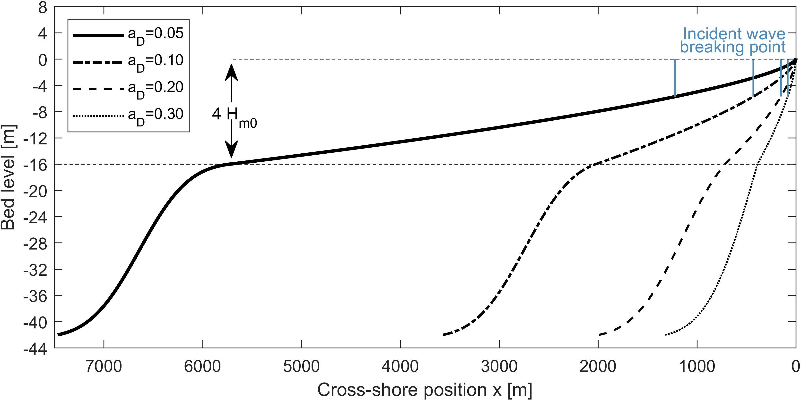
Figure 1 XBeach cross-shore profiles in the dataset of van Ormondt et al. (2021) for , , , and four variations of nearshore Dean slope (0.05, 0.10, 0.20, and 0.30) with indicated incident wave breaking point per profile in blue, adapted from van Ormondt et al. (2021).
For each point, the IG source term can be estimated using Equation 6, where the first term is obtained from the simulation results and the third term is estimated using Equation 8. Dividing the source term by the radiation stress gradient yields the shoaling parameter at each point. Note that we use the conservative shoaling component of the radiation stress gradient rather than the observed value. This is done to avoid double counting as the observed gradient in the simulations already includes the effect of friction dissipation and energy transfer to the IG component.
Data points with a relative wave height larger than 0.7 are excluded from the analysis. This was done because for these points IG wave breaking may be significant. Also, data points with a relative wave height smaller than 0.1 are excluded, since for these points in deep water the increase in IG wave height is marginal and does not yield a clear trend. The result is a set of 2,778 observations of for different combinations of and corresponding local bed slope .
The observed shoaling parameter for the training data are plotted against the local bed slope and color-coded with the relative wave height (Figure 2A). The figure reveals a trend of decreasing values of with increasing bed slopes. At mild bed slopes, the shoaling parameter is also dependent on the relative wave height . Here, lower values of , representing deeper water, result in higher shoaling parameter values. At relatively steep bed slopes, this dependency is less apparent. Therefore, the shoaling parameter is hypothesized to be a function of the local values of and :
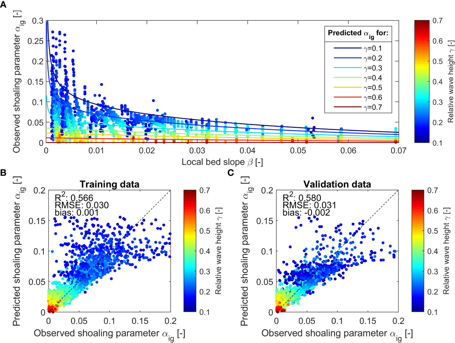
Figure 2 Observed shoaling parameter versus local bed slope and relative wave height (colored dots) and determined fits for depending on (colored solid lines) (A) and scatterplot of predicted versus observed for the training data (B) and the validation data (C).
To parameterize Equation 10, we apply a non-linear least-square fitting procedure depending on and and assume a negative exponential shape to represent the decay with increasing bed slope. The formulation distinguishes between shallower water depths () (green to red colors in Figure 2A) and deeper water depths () (blue colors in Figure 2A), which have an extra term to represent the higher observed shoaling parameter for low values of . For very shallow water depths of (dark red colors in Figure 2A), is set to 0 since those points were excluded, because IG wave dissipation is not accounted for in our simplified formulation. Furthermore, we assume that from there shoreward, there is no additional forcing to the IG waves, as the bound waves are released. For horizontal or negative bed slopes, we prescribe (Equation 12). In the case of negative bed slopes, bound IG waves may be released (Mei and Benmoussa, 1984), which we do not consider here. A maximum value of = 1 is applied to prevent spurious values for very small in combination with small values of . This gives:
The parameterization (colored lines in Figure 2A) produces an overall reasonable agreement with the observed shoaling parameter. The presence of the considerable scatter in the data introduces an inherent variability that the model may not fully capture. Furthermore, imperfections in the parametrization itself contribute to deviations from an idealized fit. Regression analysis shows an R2 coefficient of determination of 0.566, a root-mean-squared error (RMSE) of 0.03, and a bias of 0.001 for the training data (Figure 2B). The skill is similar to the validation data, which includes all validation data points including the deepest water depths, with an R2 value of 0.58 (Figure 2C).
2.2 Data
2.2.1 Synthetic data
XBeach dataset: The synthetic dataset of wave transformation and wave runup (van Ormondt et al., 2021) consists of 280 1D simulations using the incident wave-resolving XBeach non-hydrostatic two-layer model (Roelvink et al., 2009; de Ridder et al., 2021) for a large range of beach profiles and hydrodynamic conditions. The profiles are representative of sandy coasts and consist of a constant linear beach slope with angle above the mean water level. Between mean water and a depth of , the profile consists of a Dean profile (Dean, 1991) with (Figure 1), with the cross-shore distance and the elevation of the profile. In deeper water, the profile has a constant 1:50 slope up until the depth where , as recommended in de Ridder et al. (2021), with and representing the individual wave and the wave group velocity, respectively. Beyond that limit, the depth is constant. The 280 simulations consist of combinations of an offshore wave height (; 1, 2, 4, 8, 12 [m]), peak wave period (; 6, 8, 12, 16 [s]), Dean slope (; 0.05, 0.10, 0.20, 0.30 [–]), and beach slope (; 0.01, 0.02, 0.05, 0.10, 0.20 [–]). Combinations with unrealistic (too steep) wave steepness values were discarded in the dataset. At the offshore boundary, a default JONSWAP spectrum with a peak enhancement factor of 3.3 is used in XBeach. The output consists of values of incoming incident and IG rms wave heights and wave periods at selected points in the cross-shore at every 1-m depth contour interval (e.g., 1, 2, 3 m, etc.). The incoming wave signal was obtained in van Ormondt et al. (2021), using the method of Guza et al. (1984). The definition of the IG wave cutoff frequency is half the peak frequency (), the definition of which is also used throughout this study. For more details on the dataset, see van Ormondt et al. (2021). The IG wave heights are used for derivation of the parameterization describing the IG wave growth. The performance of XBeach in describing IG wave growth compared with observations is already shown in, e.g., de Ridder et al. (2021) and Roelvink et al. (2009), and for field cases, we refer to existing validations in the literature (e.g., Lashley et al., 2018; Roelvink et al., 2018).
ERA5 wave dataset: EMCWF’s ERA5 reanalysis dataset (Hersbach et al., 2020) is used for retrieving wave conditions on 13 October 1990 around the Outer Banks, USA, as used in the application case in Section 3.4. We use the significant wave height, peak wave period, and mean wave direction.
2.2.2 Laboratory data
GLOBEX dataset: The data of the GLOBEX experiments (Ruessink et al., 2013) consist of experimental laboratory experiments of wave transformation over a gently sloping linear bed with a 1:80 slope. We focus on cases A1, A2, and A3, the conditions of which can be found in Table 1 and are representative for real-world conditions of Hs = 2 m and Tp = 7 s for test A1, Hs = 4 m and Tp =10 s for A2, and Hs = 2 m and Tp =10 s for A3. From these data, we use the measured incident and IG wave heights over the profile. The incoming wave signal was obtained from de Bakker et al. (2015) using the method of Guza et al. (1984).
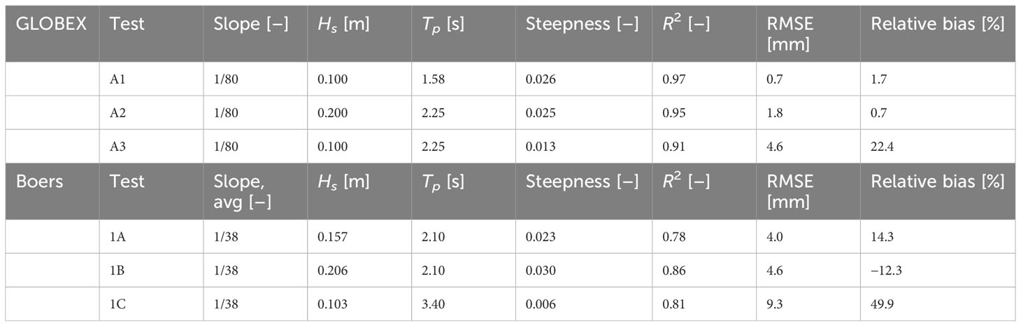
Table 1 The GLOBEX and Boers datasets detailing the (average) slope, wave conditions, and skill metrics R2, RMSE, and relative bias.
Boers dataset: The data of the experiments of Boers (1996) consist of laboratory experiments of wave transformation over a barred beach, with an average slope of about 1:38. We focus on cases 1A, 1B, and 1C, the conditions of which can be found in Table 1. From these data, we use the measured incident and IG wave heights over the profile. For both GLOBEX and Boers, to overcome data gaps and sudden jumps in the incident wave height measurements, the data are smoothed with a 10- and 5-point moving mean, respectively, to obtain useful data input as incident wave energy. The incoming wave signal was obtained in Boers (1996) using the method of Hughes (1993).
2.2.3 Field data
DELILAH dataset: The data of the DELILAH field campaign (Birkemeier et al., 1997) consist of alongshore varying 2D bathymetry data at the research facility in Duck, NC, representing the state on 13 October 1990, as, e.g., modeled by Van Dongeren (2003). The bathymetry consists of a breaker bar and small alongshore variations. From 13 October 1990, from 16:00 to 17:00, wind-still swell conditions with a significant wave height Hs of 1.81 m and a peak wave period Tp of 10.6 s were observed in 8 m water depth. These conditions are also used in other studies (e.g., Van Dongeren, 2003; Roelvink et al., 2009, 2018; Reyns et al., 2023) and are a result of Hurricane Lili. The incident wave angle is 88° from the north, corresponding to 16° from shore normal. The directional spreading factor s of the spectrum is approximately 6 (Roelvink et al., 2018), corresponding to 30.6 degrees. The local wind conditions consist of a wind speed of only 2 m/s (Birkemeier et al., 1997) and are therefore excluded in the model, as in Reyns et al. (2023). The offshore water level is 0.69 m+NGVD (National Geodetic Vertical Datum).
Topography and bathymetry datasets of North Carolina: For the application case of the Outer Banks, USA, we use the 1-m grid resolution Coastal National Elevation Database (CoNED) topographic model (Danielson et al., 2016; Tylor et al., 2022). For regions not covered by these data, the Continuously Updated Digital Elevation Model (CUDEM; CIRES, 2014), Coastal Relief Model (NOAA National Geophysical Data Center, 2001), and GEBCO (Becker et al., 2009) datasets are used.
3 Results
3.1 Validation of the infragravity wave source term against synthetic data
Validation of the prediction of IG wave transformation using the IG wave source term is performed for the synthetic profiles of VO21. For this, we include 1) a validation of the IG wave height at the incident wave breaking point and 2) a validation of the IG growth over the profile, through determining the shoaling rate.
With Equations 6, 8, 11, and 12, the IG wave growth from deep water toward nearshore can be computed. This is illustrated for one profile (Figure 3), where the shoaling parameter along the profile (Figure 3B) is determined based on the observed incident wave height (Figure 3A; black dots) and bathymetrical conditions (Figure 3C). The resulting computed IG wave height, obtained by numerically integrating Equation 6 (Figure 3A; blue line), compares well with the observed IG wave heights (Figure 3A; black triangles). Further visual inspection of the IG wave growth for more profiles and wave conditions is done in Appendix A.
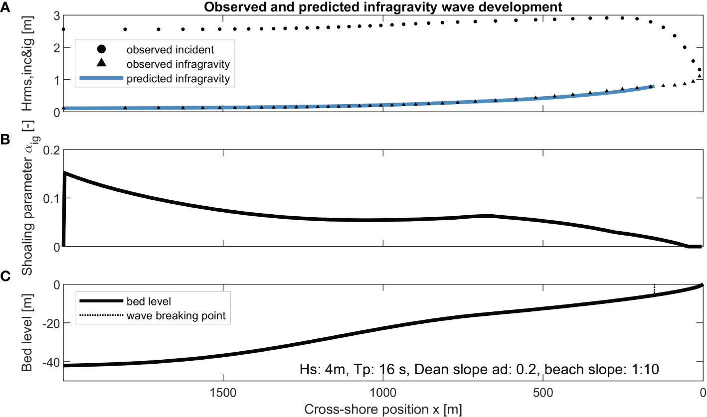
Figure 3 Example of the observed incident and infragravity wave heights (in black) and predicted infragravity wave height (in blue) (A), predicted shoaling parameter (B), and bed level with indicated incident wave breaking point (C) for XBeach simulation , , in the dataset of van Ormondt et al. (2021).
To quantify this overall 280 profiles, the observed and predicted IG wave heights at the incident wave breaking point are compared, as illustrated in Figure 4. The incident wave breaking point here is defined as the location where the incident wave height over water depth ratio equals 0.7 (dashed line in Figure 3C). For both the training data (Figure 4A) and the validation data (Figure 4B), the R2 values are similar with a low RMSE and relative bias, indicating that the results are not overfitted and the parameterization has predictive skill. For the validation profiles, this yields an R2 value of 0.964, an RMSE of 0.054 m, and a bias of −0.011 m. Overall, 94.4% of the training data and 92.9% of the validation data are within the +−25% error margins.
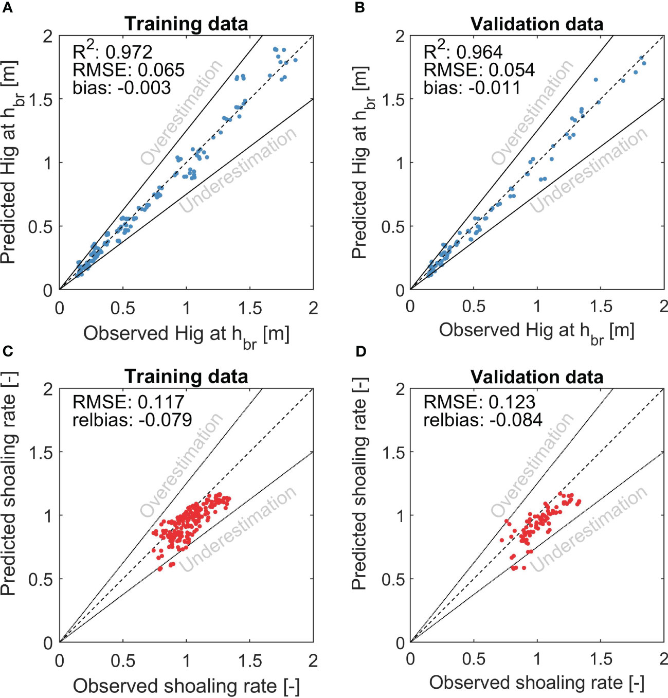
Figure 4 Comparison between predicted and observed infragravity wave heights at the wave breaking point (in blue) for the training data (A) and validation data (B), as well as a comparison between the predicted and observed shoaling rate over the entire profile (red), as fitted following the method in van Dongeren et al. (2007) for the training data (C) and the validation data (D). The dashed line shows the perfect fit line, while the solid black lines indicate the +−25% error margins.
A second validation considers the IG wave shoaling rate , defined as . This is a single parameter used to evaluate the skill of predicting the IG wave evolution. The parameter can be determined based on known values of and following the method as in van Dongeren et al. (2007). These values are taken from deep water up to the incident wave breaking point. This gives one value for the shoaling rate per profile, for both the observed and predicted data, not to be confused with the local shoaling parameter as defined in Section 2. For both the training (Figure 4C) and the validation data (Figure 4D), the shoaling rate is between 0.5 and 1.5. The performance of the training and validation data is comparable in terms of patterns and skill score, indicating that the results are not overfitted and the IG wave source term has predictive skill. The RMSE of the validation data is 0.123, and the relative bias indicates a minor underestimation of 8.4%. Overall, 96.4% of the training data and 92.9% of the validation data are within the +−25% error margins.
3.2 Validation of infragravity wave transformation in 1D against laboratory data
In this section, we compare the results of the introduced wave solver for predicting IG wave transformation (Equation 2) against laboratory data. The data are obtained from three test cases of the GLOBEX experiments (Ruessink et al., 2013) and three test cases of the Boers experiments (Boers, 1996) (see Figure 5). For each case, the IG wave transformation is computed using the observed incident wave height as input to the IG source term, rather than the values computed with Equation 1. By constraining the model in this manner, we ensure that the validation focuses solely on the IG source term and is not influenced by possible errors in the computed incident wave transformation. The wave conditions and profile characteristics are summarized in Table 1, and the model settings are summarized in Appendix B.
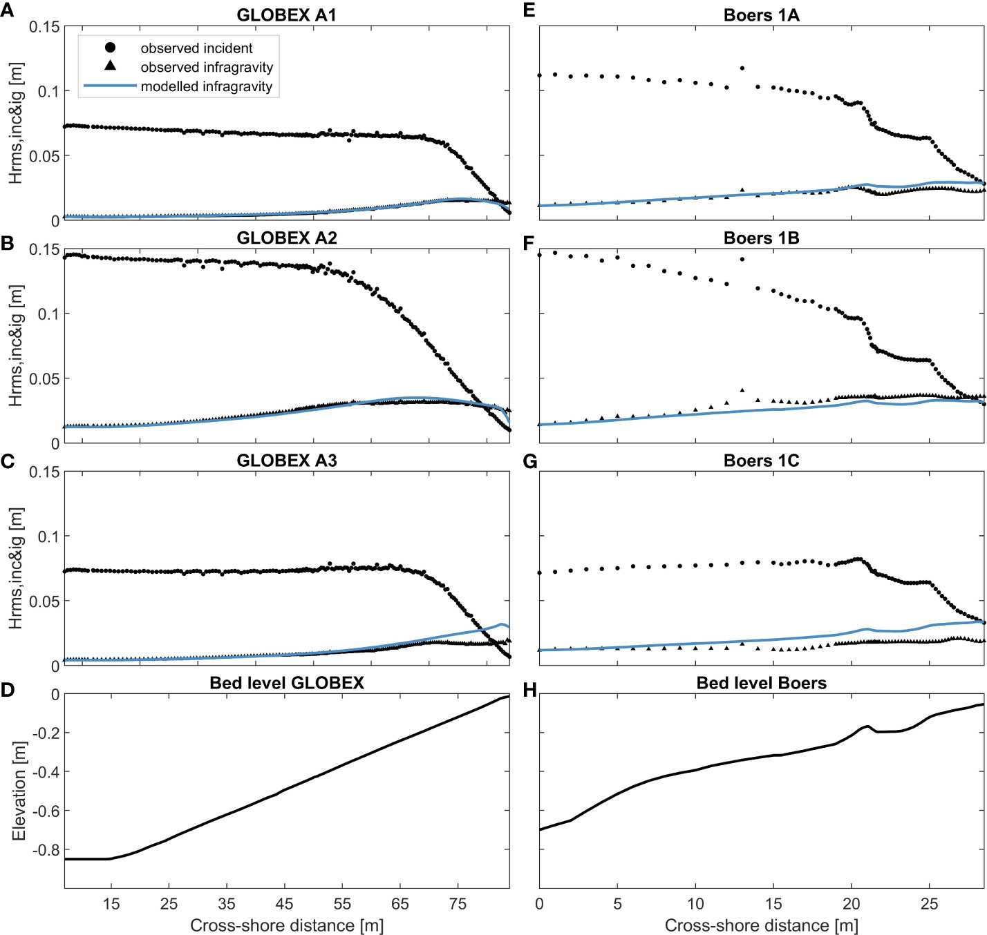
Figure 5 Observed incident and infragravity wave heights (in black) and predicted infragravity wave height (in blue) for GLOBEX tests A1 (A), A2 (B), and A3 (C) including the bed level profile (D) and for Boers tests 1A (E), 1B (F), and 1C (G) including the bed level profile (H).
The evolution of the IG wave heights for the GLOBEX test cases is quite well predicted (blue line compared with black dots), which is reflected in the skill scores (Table 1). The R2 is 0.91–0.97, RMSE 0.7–4.6 mm, and relative bias 0.7%–22.4%. The IG wave transformation is especially well predicted up until the surf zone, within the region where the incident waves have started breaking. In test A3, the IG wave breaking nearshore is underestimated.
The development of IG wave heights for the Boers tests with a barred beach profile turns out to be more difficult to model correctly (Figure 5H). For test cases 1A and 1B (Figures 5E, F), the general trend and order of magnitude are still reasonably well predicted. In test case 1A, the nearshore IG wave dissipation is underestimated. In test case 1C (Figure 5G), there is an overestimation of the predicted IG wave growth. This case combines the relatively steep profile (compared with GLOBEX), with a significantly lower wave steepness than the other Boers tests (Table 1). The overall R2 is 0.78–0.86, RMSE 4.0–9.3 mm, and relative bias −12.3% to +49.9% (Table 1).
3.3 Validation of the wave solver in 2D against field data
The prototype scale validation of the wave solver involves the DELILAH field experiment (Birkemeier et al., 1997) at Duck, NC. This site includes a non-uniform alongshore bathymetry, energetic wave conditions, non-oblique mean wave direction, and directional wave spreading. The 2D stationary wave solver (Equations 1, 2) is used to compute the incident and IG wave transformation at a spatially uniform 5-m grid resolution (as the finest resolution as used in Reyns et al., 2023). For more details on the settings of the wave solver, see Appendix B.
Spatial variations in bathymetry (Figures 6A, E) lead to alongshore and cross-shore variations in both the modeled incident (Figures 6B, D) and the modeled IG wave heights (Figures 6C, D). While the modeled incident and IG wave heights differ from the observations, the results predict the overall magnitude of wave heights reasonably well (Figures 6B–D). In between 600< x< 700 m, the incident wave height is underestimated, which can also be observed in the results of XBeach SurfBeat (Roelvink et al., 2009) and XBeach non-hydrostatic (Roelvink et al., 2018). Consequently, the IG wave height is also underestimated in that region. The offshore wave height evolution cannot be validated because of a lack of measurements. In shallow water depths landward of the breaker bar (x > 750 m, Figure 6E), the breaking of the IG waves and conservative shoaling is well captured. The RMSE over all eight measuring locations combined is 0.108 m for the incident and 0.042 m for the IG wave heights.
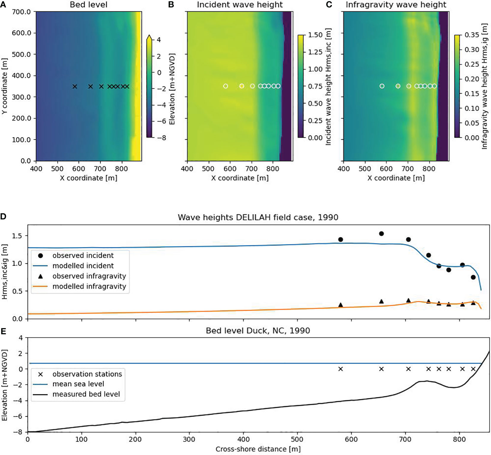
Figure 6 DELILAH case: bed level elevation including observation stations (A), observed (circles) and modeled incident wave heights (B), observed (circles) and modeled infragravity wave heights (C), observed and modeled incident and infragravity wave heights along the transect of measurements (D), and cross-shore elevation including observation stations (E).
Overall, the results have similar accuracy as Reyns et al. (2023) and Roelvink et al (Roelvink et al., 2009, 2018), who modeled the IG wave heights using a dynamic wave-resolving model.
3.4 Application of the wave solver in 2D for a large-scale domain
We now demonstrate the application of the wave solver on large domains. To this end, a model was constructed to compute nearshore IG wave conditions for 450 km of coastline. It covers the entire Outer Banks in North Carolina and most of the Virginia coastlines. We force the model with the wave conditions on 13 October 1990, using the wave reanalysis data of ERA5 (Hersbach et al., 2020), where the mean wave direction is from the east. The area model has an offshore boundary at the 200-m water depth contour at the edge of the continental shelf. A spatially varying grid resolution is used, containing 1,000 m grid cells in deep water, increasing in resolution in steps of a factor of 2, up to the finest grid cells of 31.25 m in the surf zone. The total domain has 4,493,839 active grid cells.
Various bathymetric features that affect the wave field are discernible in the bathymetry (Figure 7A). These include barrier islands, breaker bars, and shoals. Behind the Cape Lookout Shoals (orange triangle in Figure 7B), a sheltered area is visible where the wave height is lower. The computed IG wave height field (Figure 7C) shows that the highest IG wave heights occur close to the shore, where the incident wave shoaling is the strongest. The shoaling is particularly strong just north of Duck (red triangle in Figure 7C), where a range of nearshore bathymetric features lead to large changes in radiation stress, leading to stronger IG wave growth. At the Cape Lookout Shoals, the waves from the east shoal up and generate IG waves. In general, the patterns of the IG wave fields are consistent with the bed level and incident wave height changes.
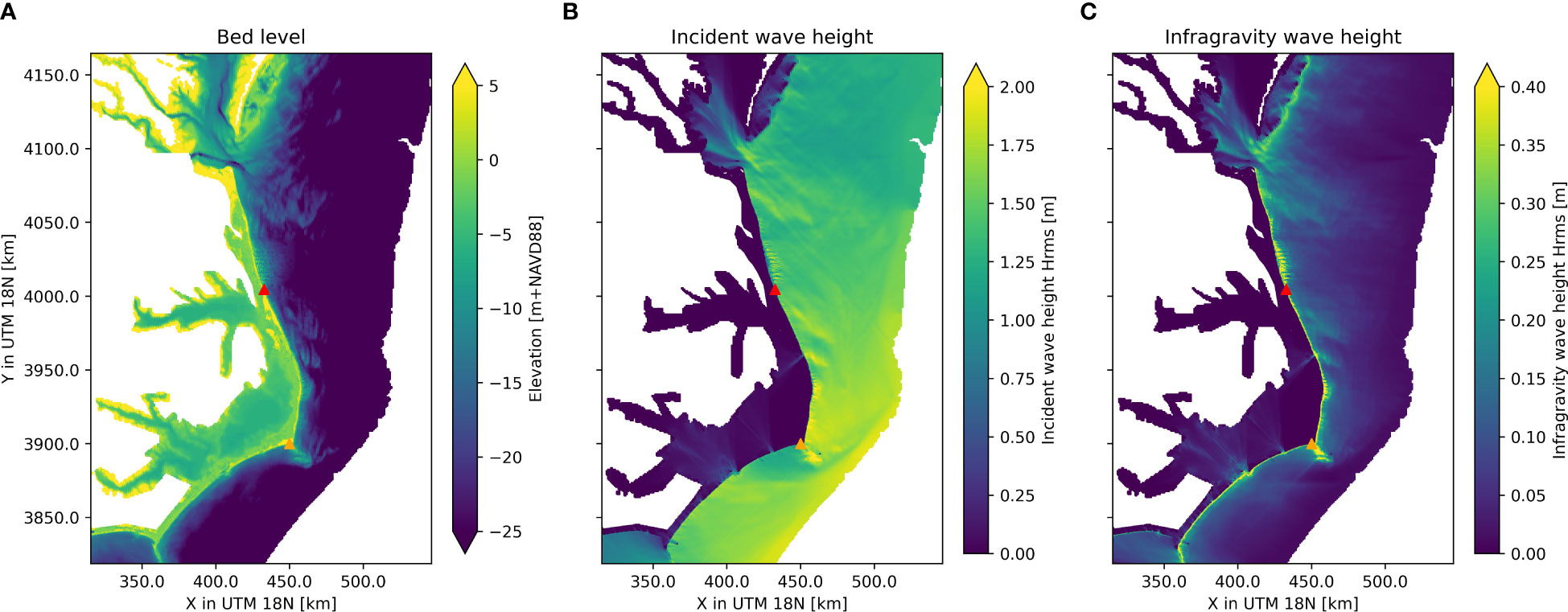
Figure 7 Outer Banks case: bed level elevation (A), modeled incident wave heights (B), and modeled infragravity wave heights (C) for the Outer Banks upscaling demonstration model. Duck, NC, is indicated in the red triangle and Cape Lookout Shoals, NC, in the orange triangle.
The computation of a single stationary wave field (combining both incident and IG waves) of 4.5 million grid cells takes mere seconds on a regular laptop PC. This is significantly faster than computations by advanced wave-group-resolving numerical models that would take hours to days to calculate this for a domain of this size.
4 Discussion
The presented wave solver provides reasonable to good estimates of the nearshore IG wave conditions for large spatial scales and with a low computational expense. Since a reduced complexity approach is taken, it is not a full description of the physics involving the generation of IG waves (as is the case for most numerical models). The main limitations, assumptions, and discussion points of both the IG wave source term and the full 2D wave solver are outlined below:
4.1 Limitations of the infragravity wave source term
The proposed IG wave source term using a parameterization for the shoaling parameter , based on the local bed slope and wave height over water depth ratio, is a simplified physical description. Therefore, the goodness of the fit of the parameterization of the shoaling parameters is not very high with an R2 score of 0.580 (Section 2.1.3). However, when predicting the IG wave development from offshore to nearshore, the uncertainty in the exact value of matters less, which is indicated by an R2 value of 0.964 in estimating the IG wave height at the incident wave breaking point and a small bias of 1.1 cm (Section 3.1).
The dataset of VO21 used for deriving and validating the parameterization consists of 1D XBeach non-hydrostatic two-layer model results. Shore normal 1D models overestimate the IG wave growth compared with the 2D XBeach models (van Ormondt et al., 2021; McCall et al., 2023), because all energy is forced into the shore normal wave direction and directional spreading is not considered. Furthermore, the parameterization assumes a JONSWAP spectral shape in the incident wave band, as is used in the VO21 dataset, which is applicable to nearshore conditions. The evolution of IG wave heights and the corresponding IG wave source term may differ for variations of this spectral shape and subsequent groupiness. The effect of directional spreading and wave groupiness on IG wave shoaling requires further investigation.
In the IG source term, the shoaling parameter (and therefore the source term itself) becomes zero for negative bed slopes (Equation 12). These occur where the water depth increases in the wave propagation direction, e.g., on the landward side of a submerged breaker bar or when IG waves enter a deeper tidal channel after passing a shallow shoal (Reniers and Zijlema, 2022). These conditions are not present in the VO21 dataset from which the parameterization was derived. The choice to set the source term to zero for these cases was made to keep the IG source term simple and not have to account for the possibility that bound IG waves may become released. This aspect of the parameterization is however likely inaccurate and should be further investigated.
No clear correlation was found in the VO21 dataset between incident wave steepness and the IG source term. The steepness is therefore not explicitly considered in our parameterization. However, some cases with low wave steepness, such as Boers test 1C, showed an overestimation of the predicted IG wave growth. It is recommended that the effect of wave period and wave steepness on IG wave transformation is further investigated.
4.2 Limitations of the wave solver
In the wave solver, IG wave-breaking dissipation was included using the formulation of Baldock et al. (1998). This formulation was derived for sea swell and has not been validated for IG waves. Further investigation into the validity of the formulation is needed and might also improve results, e.g., GLOBEX test A3 and Boers tests 1A and 1C, which would benefit from introducing more IG wave breaking.
Break point forcing may contribute significantly to IG wave generation at steep rocky coasts and coral-reef-lined coastlines (Battjes et al., 2004; Van Dongeren et al., 2013). A source term to represent this process has not yet been implemented in the wave solver. As a result, the solver’s applicability is currently limited to coasts with relatively mild slopes.
As with other numerical models, the present wave solver requires a relatively good estimate of the nearshore bathymetry, resolving, e.g., breaker bars. This in contrast with other approaches that use a certain mean (surf zone or beach) bed slope to represent the coastal profile. These bathymetric details are not covered in coarser global datasets (e.g., GEBCO) or derived profile datasets (e.g., Athanasiou et al., 2019, 2023). However, the sensitivity between estimates of IG wave growth derived from using a detailed or coarser bathymetry has not been assessed and could be considered for future work.
The presented wave solver has not yet been validated in 2D during extreme conditions as the significant wave height of 1.8 m for Duck was relatively limited. However, because the IG wave source term has been derived and validated based on conditions in XBeach with significant wave heights up to 12 m, the derived wave solver is assumed to be valid for extreme events along sandy beach coastlines. Field validation could be considered as a direction for future research.
5 Conclusions
In this study, we introduce an efficient stationary wave energy solver designed to estimate the evolution of incident and IG waves from offshore to the nearshore, specifically for mildly sloping coasts. This wave solver can be used to generate nearshore IG wave boundary conditions to drive overland flood models at large scales and with little computational expense.
The new wave solver builds upon the stationary wave energy balance for incident wave energy. The formulations are extended to also include the IG wave energy balance. For this purpose, we introduce an IG wave source term that describes the energy transfer from incident to IG waves. This term acts as a sink term for the incident waves and as a complementary source term for the IG waves. The IG wave source term is simplified using an IG wave shoaling parameter . Observed values of this parameter are obtained from a synthetic dataset of covering a wide range of wave conditions and beach profiles. These are used to derive an empirical relation, which describes the shoaling parameter as a function of the local bed slope and the incident wave height over water depth ratio . While the parameterization of exhibits some scatter relative to observed values (R2 value of 0.566), it captures the general trend without overfitting. Most importantly, employing this parameterization accurately predicts the IG wave source term and subsequent IG wave height evolution across all profiles in the validation dataset. The shoaling rate over the cross-shore profile is predicted with an RMSE of 0.123 with 92.9% of the validation data falling within the +−25% error margins. IG wave heights at the incident wave breaking point are predicted with high accuracy, indicated by an R2 value of 0.96 and an RMSE of 0.05 m.
With this parameterization, the wave solver can estimate IG wave transformation based on offshore incident wave heights and local bathymetry as input. The wave solver is shown to be able to predict the evolution of IG wave heights for three laboratory tests of GLOBEX (RMSE between 0.7 and 4.6 mm, R2 of 0.91–0.97) and for the more complex bed level of three laboratory tests of Boers (RMSE between 4.0 and 9.3 mm, R2 of 0.78–0.86). Additionally, validation of the wave solver in 2D using the 1990 DELILAH field case observations at Duck, NC, USA, yields results that align well with those obtained with computationally expensive dynamic wave models. Predictions of incident wave height yield an RMSE of 0.11 m, while IG wave height estimates exhibit an RMSE of 0.04 m.
The large-scale applicability of the wave solver is further demonstrated by modeling the entire Outer Banks, North Carolina, coastline in the USA, covering 450 km of coastline from 200 m water depth up to the coast. For this model, consisting of 4.5 million grid cells, the wave solver can calculate IG wave conditions for the entire domain within seconds.
The presented wave solver makes it possible to include IG wave-driven flooding in large-scale compound flood modes. Its computational efficiency, with results in seconds, stands in contrast to process-based wave-resolving models, which require hours to days to run. In future work, this wave solver will be used to force a reduced complexity model (SFINCS), for IG wave-resolving flood hazard modeling at the national to continental scales.
Data availability statement
The developed wave solver has been integrated in the fast compound flood model SFINCS, which is openly available from https://www.deltares.nl/en/software-and-data/products/sfincs. The source code of the coupled model with wave solver and infragravity source term as developed in this paper is available from https://github.com/Deltares/SFINCS/releases/tag/v2.0.5-alpha-branch-sfincs_snapwave_ig_2024_02_10 and will be incorporated in future releases of SFINCS. The data analyzed in this study are subject to the following licenses/restrictions: The used dataset of XBeach simulations was not made available open source by van Ormondt et al. (2021); however, the data are generated using the open-source XBeach model. Access to the dataset can be requested on a personal basis. Requests to access these datasets should be directed to bWFhcnRlbi52YW5vcm1vbmR0QGRlbHRhcmVzLXVzYS51cw==.
Author contributions
TL: Conceptualization, Formal analysis, Funding acquisition, Investigation, Methodology, Project administration, Software, Validation, Visualization, Writing – original draft. MO: Conceptualization, Methodology, Investigation, Software, Writing – review & editing. AD: Conceptualization, Methodology, Supervision, Writing – original draft, Writing – review & editing. JA: Supervision, Writing – review & editing, Funding acquisition. SM: Supervision, Writing – review & editing.
Funding
The author(s) declare that financial support was received for the research, authorship, and/or publication of this article. This project has been funded by EU ERC COASTMOVE nr 884442 and by Deltares SITO-IS research funding under Moonshot 2 – Flooding.
Acknowledgments
We would like to thank Johan Reyns for providing the input data as used in the Duck field case, as well as Carola Seyfert for making the initial version of the model setup. Permission to use the data provided by the Field Research Facility of the U.S. Army Engineer Waterways Experiment Station’s Coastal Engineering Research Center is greatly appreciated.
Conflict of interest
The authors declare that the research was conducted in the absence of any commercial or financial relationships that could be construed as a potential conflict of interest.
Publisher’s note
All claims expressed in this article are solely those of the authors and do not necessarily represent those of their affiliated organizations, or those of the publisher, the editors and the reviewers. Any product that may be evaluated in this article, or claim that may be made by its manufacturer, is not guaranteed or endorsed by the publisher.
References
Athanasiou P., Van Dongeren A., Giardino A., Vousdoukas M., Antolinez J. A.A., Ranasinghe R. (2022). Estimating dune erosion at the regional scale using a meta-model based on neural networks. Natural Hazards Earth Sys. Sci. 22, 3897–39155. doi: 10.5194/nhess-22-3897-2022
Athanasiou P., Van Dongeren A., Giardino A., Vousdoukas M., Gaytan-Aguilar S., Ranasinghe R. (2019). Global distribution of nearshore slopes with implications for coastal retreat. Earth Sys. Sci. Data 11, 1515–1295. doi: 10.5194/essd-11-1515-2019
Athanasiou P., van Dongeren A., Pronk M., Giardino A., Vousdoukas M., Ranasinghe R. (2023). Global Coastal Characteristics (GCC): A global dataset of geophysical, hydrodynamic, and socioeconomic coastal indicators. Earth Syst. Sci. Data Discuss. [preprint]. doi: 10.5194/essd-2023-313. in review.
Baldock T. E., Holmes P., Bunker S., Van Weert P. (1998). Cross-shore hydrodynamics within an unsaturated surf zone. Coast. Eng. 34, 173–196. doi: 10.1016/S0378-3839(98)00017-9
Bates P. D., Horritt M. S., Fewtrell T. J. (2010). A simple inertial formulation of the shallow water equations for efficient two-dimensional flood inundation modelling. J. Hydrol. 387, 33–45. doi: 10.1016/j.jhydrol.2010.03.027
Battjes J. A., Bakkenes H. J., Janssen T. T., van Dongeren A. R. (2004). Shoaling of subharmonic gravity waves. J. Geophys. Res. 109, C02009. doi: 10.1029/2003JC001863
Becker J. J., Sandwell D. T., Smith W. H. F., Braud J., Binder B., Depner J., et al. (2009). Global bathymetry and elevation data at 30 arc seconds resolution: SRTM30_PLUS. Mar. Geodesy 32, 355–371. doi: 10.1080/01490410903297766
Bertin X., de Bakker A., van Dongeren A., Coco G., André G., Ardhuin F., et al. (2018). Infragravity waves: from driving mechanisms to impacts. Earth-Sci. Rev. 177, 774–799. doi: 10.1016/j.earscirev.2018.01.002
Birkemeier W. A., Donoghue C., Long C. E., Hathaway K. K., Baron C. F. (1997). 1990 DELILAH Nearshore Experiment: Summary Report. Techreport CHL-97-24 (Vicksburg, Mississippi, USA: US Army Engineer Waterways Experiment Station).
Boers M. (1996). “Simulation of a Surf Zone with a Barred Beach. Report 1. Wave Heights and Wave Breaking,” in Communications on Hydraulic and Geotechnical Engineering (Delft: Delft). Available at: http://resolver.tudelft.nl/uuid:22dfbc0a-adf8-44cb-96599d0a366c88d6.
Booij N. R. R. C., Ris R. C., Holthuijsen L. H. (1999). A third-generation wave model for coastal regions: 1. model description and validation. J. geophysical research: Oceans 104 (C4), 7649–7666. doi: 10.1029/98JC02622
Camus P., Haigh I. D., Nasr A. A., Wahl T., Darby S. E., Nicholls R. J. (2021). Regional analysis of multivariate compound coastal flooding potential around Europe and environs: sensitivity analysis and spatial patterns. Natural Hazards Earth Sys. Sci. 21, 2021–2405. doi: 10.5194/nhess-21-2021-2021
CIRES (2014). Cooperative institute for research in environmental sciences (CIRES) at the university of Colorado, boulder. 2014: continuously updated digital elevation model (CUDEM). NOAA Natl. Centers Environ. Inf. doi: 10.25921/DS9V-KY35
Dalinghaus C., Coco G., Higuera P. (2022). A predictive equation for wave setup using genetic programming. Nat. Hazards Earth Syst. Sci.. 23, 2157–2169. doi: 10.5194/nhess-2022-221
Danielson J. J., Poppenga S. K., Brock J. C., Evans G. A., Tyler D. J., Gesch D. B., et al. (2016). Topobathymetric elevation model development using a new methodology: coastal national elevation database. J. Coast. Res. 76, 75–89. doi: 10.2112/SI76-008
Dean R. G. (1991). Equilibrium beach profiles: characteristics and applications. J. Coast. Res. 7, 53–84.
Dean R. G., Dalrymple R. A. (1991). “Water Wave Mechanics for Engineers and Scientists,” in Advanced Series on Ocean Engineering (Singapore: World Scientific), vol. 2. doi: 10.1142/1232
de Bakker A. T. M., Herbers T. H. C., Smit P. B., Tissier M. F. S., Ruessink B. G. (2015). Nonlinear infragravity–wave interactions on a gently sloping laboratory beach. J. Phys. Oceanogr. 45, 589–6055. doi: 10.1175/JPO-D-14-0186.1
De Kleermaeker S., Leijnse T., Morales Y., Druery C., Maguire S. (2022). Developing a Real-Time Data and Modelling Framework for Operational Flood Inundation Forecasting in Australia (Brisbane: Engineers Australia). doi: 10.3316/informit.916755150845355
de Ridder M. P., Smit P. B., van Dongeren A., McCall R. T., Nederhoff K., Reniers A. J. H. M. (2021). Efficient two-layer non-hydrostatic wave model with accurate dispersive behaviour. Coast. Eng. 164, 103808. doi: 10.1016/j.coastaleng.2020.103808
Diermanse F., Roscoe K., Van Ormondt M., Leijnse T., Winter G., Athanasiou P. (2023). Probabilistic compound flood hazard analysis for coastal risk assessment: A case study in Charleston, South Carolina. Shore Beach 91 (2), 9–18. doi: 10.34237/1009122
Eilander D., Couasnon A., Leijnse T., Ikeuchi H., Yamazaki D., Muis S., et al. (2022). A globally-applicable framework for compound flood hazard modeling. Nat. Hazards Earth Syst. Sci.. 23, 823–846. doi: 10.5194/egusphere-2022-149
Emanuel K. A. (2013). Downscaling CMIP5 climate models shows increased tropical cyclone activity over the 21st century. Proc. Natl. Acad. Sci. 110, 12219–12224. doi: 10.1073/pnas.1301293110
Fiedler J. W., Brodie K. L., McNinch J. E., Guza R. T. (2015). Observations of runup and energy flux on a low-slope beach with high-energy, long-period ocean swell. Geophys. Res. Lett. 42, 9933–9415. doi: 10.1002/2015GL066124
Gaido Lasserre C., Reguero B., Nederhoff K., Storlazzi C. D., Leijnse T., Van Dongeren A., et al. (2020). From Regional Flood Risk Analysis to Local: Comparing Coastal Flooding in Miami Beach with XBeach and SFINCS. Available at: https://agu2020fallmeeting-agu.ipostersessions.com/?s=30-38-5A-0C-8E-22-C8-84-CC-46-3C-95-18-80-C2-76&token=5r05NKrASrFrnkybTgXa4Y_XvgfV233Dazers0d2Zzo.
Grimley L. E., Sebastian A., Leijnse T., Eilander D., Ratcliff J., Luettich R. A. (2023). Determining the Relative Contributions of Runoff and Coastal Processes to Flood Exposure across the Carolinas during Hurricane Florence. Journal is Water Resources Research. doi: 10.22541/essoar.170067213.37538296/v1, in review.
Guza R. T., Thornton E. B. (1982). Swash oscillations on a natural beach. J. Geophys. Res. 87, 483. doi: 10.1029/JC087iC01p00483
Guza R. T., Thornton E. B., Holman R. A. (1984). “Swash on steep and shallow beaches,” in Paper Presented at 19th Coastal Engineering Conference, Houston, TX, USA, Am. Soc. of Civ. Eng.
Henderson S. M., Bowen (2002). Observations of surf beat forcing and dissipation. J. Geophys. Res. 107, 3193. doi: 10.1029/2000JC000498
Herbers T. H. C., Elgar S., Guza R. T. (1994). Infragravity-frequency (0.005–0.05 hz) motions on the shelf. Part I: forced waves. J. Phys. Oceanogr. 24, 917–275. doi: 10.1175/1520-0485(1994)024<0917:IFHMOT>2.0.CO;2
Hersbach H., Bell B., Berrisford P., Hirahara S., Horányi A., Muñoz-Sabater J., et al. (2020). The ERA5 global reanalysis. Q. J. R. Meteorol. Soc. 146, 1999–2049. doi: 10.1002/qj.3803
Hughes S. A. (1993). Laboratory wave reflection analysis using co-located gages. Coast. Eng. 20, 223–247. doi: 10.1016/0378-3839(93)90003-Q
Janssen T. T., Battjes J. A., van Dongeren A. R. (2003). Long waves induced by short-wave groups over a sloping bottom. J. Geophys. Res. 108, 3252. doi: 10.1029/2002JC001515
Jones B., O’Neill B. C. (2016). Spatially explicit global population scenarios consistent with the shared socioeconomic pathways. Environ. Res. Lett. 11, 84003. doi: 10.1088/1748-9326/11/8/084003
Kirezci E., Young I. R., Ranasinghe R., Muis S., Nicholls R. J., Lincke D., et al. (2020). Projections of global-scale extreme sea levels and resulting episodic coastal flooding over the 21st century. Sci. Rep. 10, 116295. doi: 10.1038/s41598-020-67736-6
Lashley C. H., Roelvink D., van Dongeren A., Buckley M. L., Lowe R. J. (2018). Nonhydrostatic and surfbeat model predictions of extreme wave run-up in fringing reef environments. Coast. Eng. 137, 11–27. doi: 10.1016/j.coastaleng.2018.03.007
Leijnse T., De Goede R., Ormondt M. V., Lemans M., Hegnauer M., Eilander D., et al. (2023a). Developing large scale and fast compound flood models for Australian coastlines. Coast. Eng. Proc. 37, 49. doi: 10.9753/icce.v37.management.49
Leijnse T., Nederhoff K., Thomas J., Parker K., van Ormondt M., Erikson L., et al. (2023b). Rapid modeling of compound flooding across broad coastal regions and the necessity to include rainfall driven processes: A case study of Hurricane Florence (2018). In Coastal Sediments 2023: The Proceedings of the Coastal Sediments 2023, 2576–2584. doi: 10.1142/9789811275135_0235
Leijnse T., van Ormondt M., Nederhoff K., van Dongeren A. (2021). Modeling compound flooding in coastal systems using a computationally efficient reduced-physics solver: including fluvial, pluvial, tidal, wind- and wave-driven processes. Coast. Eng. 163, 103796. doi: 10.1016/j.coastaleng.2020.103796
Longuet-Higgins M. S., Stewart R. W. (1964). Radiation stresses in water waves; a physical discussion, with applications. Deep Sea Res. Oceanogr. Abst. 11, 529–625. doi: 10.1016/0011-7471(64)90001-4
Masselink G. (1995). Group bound long waves as a source of infragravity energy in the surf zone. Continent. Shelf Res. 15, 1525–1547. doi: 10.1016/0278-4343(95)00037-2
McCall R., Van Santen R., Wilmink R., De Bakker A., Steetzel H., Pluis S., et al. (2023). “Accounting for directional wave spreading effects on infragravity wave growth in a 1d dune erosion model,” in Coastal Sediments 2023 (WORLD SCIENTIFIC, New Orleans, LA, USA). doi: 10.1142/9789811275135_0183
McGranahan G., Balk D., Anderson B. (2007). The rising tide: assessing the risks of climate change and human settlements in low elevation coastal zones. Environ. Urban. 19, 17–375. doi: 10.1177/0956247807076960
McMichael C., Dasgupta S., Ayeb-Karlsson S., Kelman I. (2020). A review of estimating population exposure to sea-level rise and the relevance for migration. Environ. Res. Lett. 15, 1230055. doi: 10.1088/1748-9326/abb398
Mei C. C., Benmoussa C. (1984). Long waves induced by short-wave groups over an uneven bottom. J. Fluid Mechanics 139, 219–235. doi: 10.1017/S0022112084000331
Merkens J.-L., Reimann L., Hinkel J., Vafeidis A. T. (2016). Gridded population projections for the coastal zone under the shared socioeconomic pathways. Global Planet. Change 145, 57–66. doi: 10.1016/j.gloplacha.2016.08.009
Mousavi M. E., Irish J. L., Frey A. E., Olivera F., Edge B. L. (2011). Global warming and hurricanes: the potential impact of hurricane intensification and sea level rise on coastal flooding. Climatic Change 104, 575–597. doi: 10.1007/s10584-009-9790-0
Muis S., Verlaan M., Winsemius H. C., Aerts J. C. J. H., Ward P. J. (2016). “A Global Reanalysis of Storm Surges and Extreme Sea Levels.” Nat. Commun. 7 (1), 11969. doi: 10.1038/ncomms11969
Nederhoff K., Crosby S. C., Van Arendonk N. R., Grossman E. E., Tehranirad B., Leijnse T., et al. (2024a). Dynamic modeling of coastal compound flooding hazards due to tides, extratropical storms, waves, and sea-level rise: A case study in the Salish sea, Washington (USA). Water 16, 3465. doi: 10.3390/w16020346
Nederhoff K., van Ormondt M., Veeramony J., van Dongeren A., Antolínez J. A.Á., Leijnse T., et al. (2024b). Accounting for uncertainties in forecasting tropical-cyclone-induced compound flooding. Geosci. Model Dev. 17, 1789–1811. doi: 10.5194/gmd-17-1789-2024
Neumann B., Vafeidis A. T., Zimmermann J., Nicholls R. J. (2015). Future coastal population growth and exposure to sea-level rise and coastal flooding - A global assessment. PloS One 10, e01185715. doi: 10.1371/journal.pone.0118571
NOAA National Geophysical Data Center (2001). U.S. Coastal relief model vol.3 - Florida and east gulf of Mexico. Accessed 6/30/21. Natl. Geophys. Data Center NOAA. doi: 10.7289/V5W66HPP
Parker K., Erikson L., Thomas J., Nederhoff K., Barnard P., Muis S. (2023). Relative contributions of water-level components to extreme water levels along the US southeast Atlantic coast from a regional-scale water-level hindcast. Natural Hazards. doi: 10.1007/s11069-023-05939-6
Pearson S. G., Storlazzi C. D., van Dongeren A. R., Tissier M. F. S., Reniers A. J. H. M. (2017). A bayesian-based system to assess wave-driven flooding hazards on coral reef-lined coasts. J. Geophys. Res.: Oceans 122, 10099–10117. doi: 10.1002/2017JC013204
Phillips O. M. (1977). The Dynamics of the Upper Ocean. 2nd ed. (Cambridge-London-New York-Melbourne: Cambridge University Press).
Qiang Y., He J., Xiao T., Lu W., Li J., Zhang L. (2021). Coastal Town Flooding upon Compound Rainfall-Wave Overtopping-Storm Surge during Extreme Tropical Cyclones in Hong Kong. J. Hydrol.: Region. Stud. 37, 100890. doi: 10.1016/j.ejrh.2021.100890
Reniers A., Zijlema M. (2022). SWAN SurfBeat-1D. Coast. Eng. 172, 104068. doi: 10.1016/j.coastaleng.2021.104068
Reyns J., McCall R., Ranasinghe R., van Dongeren A., Roelvink D. (2023). Modelling wave group-scale hydrodynamics on orthogonal unstructured meshes. Environ. Model. Softw. 162, 105655. doi: 10.1016/j.envsoft.2023.105655
Roeber V., Bricker J. D. (2015). Destructive Tsunami-like Wave Generated by Surf Beat over a Coral Reef during Typhoon Haiyan. Nat. Commun. 6, 7854. doi: 10.1038/ncomms8854
Roeber V., Cheung K. F., Kobayashi M. H. (2010). Shock-capturing boussinesq-type model for nearshore wave processes. Coast. Eng. 57, 407–235. doi: 10.1016/j.coastaleng.2009.11.007
Roelvink D., McCall R., Mehvar S., Nederhoff K., Dastgheib A. (2018). Improving predictions of swash dynamics in XBeach: the role of groupiness and incident-band runup. Coast. Eng. 134, 103–123. doi: 10.1016/j.coastaleng.2017.07.004
Roelvink D., Reniers A., van Dongeren A., van Thiel de Vries J., McCall R., Lescinski J. (2009). Modelling storm impacts on beaches, dunes and barrier islands. Coast. Eng. 56, 1133–1152. doi: 10.1016/j.coastaleng.2009.08.006
Ruessink G., Michallet H., Bonneton P., Mouazé D., Lara J. L., Silva P. A., et al. (2013). GLOBEX: Wave dynamics on a gently sloping laboratory beach. In 7th International Conference on Coastal Dynamics, 1351–1362.
Schäffer H. A. (1993). Infragravity waves induced by short-wave groups. J. Fluid Mech. 247, 551–588. doi: 10.1017/S0022112093000564
Stockdon H. F., Holman R. A., Howd P. A., Sallenger A. H. (2006). Empirical parameterization of setup, swash, and runup. Coast. Eng. 53, 573–885. doi: 10.1016/j.coastaleng.2005.12.005
Stocker T. (2014). Climate Change 2013: The Physical Science Basis: Working Group I Contribution to the Fifth Assessment Report of the Intergovernmental Panel on Climate Change (New York: Cambridge University Press).
Svendsen I. A. (1984). Wave heights and set-up in a surf zone. Coast. Eng. 8, 303–329. doi: 10.1016/0378-3839(84)90028-0
Swart D. H. (1974). Offshore Sediment Transport and Equilibrium Beach Profiles (Netherlands: Delft Hydraul. Lab., Delft). Publ. 131.
Tebaldi C., Ranasinghe R., Vousdoukas M., Rasmussen D. J., Vega-Westhoff B., Kirezci E., et al. (2021). Extreme sea levels at different global warming levels. Nat. Climate Change 11, 746–515. doi: 10.1038/s41558-021-01127-1
Tolman H. L. (2002). Distributed-memory concepts in the wave model WAVEWATCH III. Parallel Computing 28 (1), 35–52. doi: 10.1016/S0167-8191(01)00130-2
Tyler D., Cushing W. M., Danielson J. J., Poppenga S., Beverly S., Shogib R. (2022). Topobathymetric Model of the Coastal Carolinas 1851 to 2020 (Ver 2.0, January 2023): U.S. Geological Survey Data Release. doi: 10.5066/P9MPA8K0
US Army Corps Of Engineers (2002). US Army Corps of Engineers: Coastal engineering manual, report number 11102-1100. (Washington, DC: US Army Corps of Engineers), 477 pp.
Van Dongeren A. (2003). Numerical modeling of infragravity wave response during DELILAH. J. Geophys. Res. 108, 3288. doi: 10.1029/2002JC001332
van Dongeren A., Battjes J., Janssen T., van Noorloos J., Steenhauer K., Steenbergen G., et al. (2007). Shoaling and shoreline dissipation of low-frequency waves. J. Geophys. Res. 112, C02011. doi: 10.1029/2006JC003701
Van Dongeren A., Lowe R., Pomeroy A., Trang D. M., Roelvink D., Symonds G., et al. (2013). Numerical modeling of low-frequency wave dynamics over a fringing coral reef. Coast. Eng. 73, 178–190. doi: 10.1016/j.coastaleng.2012.11.004
van Oosterhout L., Koks E., Van Beukering P., Schep S., Tiggeloven T., Van Manen S., et al. (2023). An integrated assessment of climate change impacts and implications on bonaire. Econ. Disasters Climate Change. 7, 147–178. doi: 10.1007/s41885-023-00127-z
van Ormondt M., Roelvink D., van Dongeren A. (2021). A model-derived empirical formulation for wave run-up on naturally sloping beaches. J. Mar. Sci. Eng. 9, 11855. doi: 10.3390/jmse9111185
Vousdoukas M. I., Voukouvalas E., Mentaschi L., Dottori F., Giardino A., Bouziotas D., et al. (2016). Developments in large-scale coastal flood hazard mapping. Natural Hazards Earth Sys. Sci. 16, 1841–1535. doi: 10.5194/nhess-16-1841-2016
Wahl T., Jain S., Bender J., Meyers S. D., Luther M. E. (2015). Increasing risk of compound flooding from storm surge and rainfall for major US cities. Nat. Clim Change 5, 1093–1097. doi: 10.1038/nclimate2736
Ward P. J., Couasnon A., Eilander D., Haigh I. D., Hendry A., Muis S., et al. (2018). Dependence between high sea-level and high river discharge increases flood hazard in global deltas and estuaries. Environ. Res. Lett. 13, 0840125. doi: 10.1088/1748-9326/aad400
Winter G., Storlazzi C., Vitousek S., van Dongeren Ap., McCall R., Hoeke R., et al. (2020). Steps to develop early warning systems and future scenarios of storm wave-driven flooding along coral reef-lined coasts. Front. Mar. Sci. 7. doi: 10.3389/fmars.2020.00199
Zijlema M., Stelling G., Smit P. (2011). SWASH: an operational public domain code for simulating wave fields and rapidly varied flows in coastal waters. Coast. Eng. 58, 992–10125. doi: 10.1016/j.coastaleng.2011.05.015
Appendix A: further inspection of infragravity wave growth for profiles
To further analyze the results of Section 3.1, an additional visual inspection of the results of IG wave development for many profiles is performed. The IG wave development for many profiles (Figure A1) shows how well the prediction compares to the observations of XBeach. For the beach slope of 0.05, all profiles have been shown, with varying wave height, wave period, and nearshore Dean slope as in elevation . To simplify the comparison, the IG wave height on the y-axis is normalized by the offshore incident wave height, and the dimensionless is used on the x-axis. Also, the different incident wave heights are colored differently (blue for 1 m, green for 2 m, brown for 4 m, orange for 8 m, and red for 12 m). Note that in VO21, combinations with unrealistically steep wave steepness were not included (e.g., a significant wave height of 12 m with a peak wave period of 6 s was excluded), leaving more combinations for lower wave heights than higher ones.
The rate and pattern of IG wave growth depend significantly on the combination of offshore wave period and the local bed slope. For a wave height of 2 m for instance, the maximum IG wave height is higher for a higher wave period (equals lower wave steepness), and IG wave breaking occurs at a higher value of n. Additionally, this pattern differs again when looking at different Dean beach slopes, which mainly influences at what value of n the main amplification in IG wave shoaling occurs. Comparing profiles with different wave heights directly is harder because of the different wave steepness involved.
In general, in deeper water, the IG wave growth is well predicted for all profiles up to a value of n of ~0.9. More nearshore, the performance depends on the combination of wave steepness and Dean slope. The profiles with a Dean slope of 0.20 and 0.30 match well also nearshore. For a Dean slope of 0.10, this is still the case for a higher wave steepness, but not always for the lowest wave steepness in the set. For a mild Dean slope of 0.05, the profiles with a low wave steepness underestimate the IG wave growth nearshore more significantly. Thus, there is a dependence on the bed slopes, since for two simulations with an Hs = 2 m and a Tp = 16 s for instance; with a Dean slope of 0.30, the IG growth is fully captured, while for Dean slope of 0.05, this is not fully the case. The results show that there is a group of profiles with very mild dean slopes and low wave steepness, where the predicted IG evolution is a bit underestimated.
Appendix B: boundary conditions and model settings of the wave solver
Boundary conditions of infragravity waves
To describe the full evolution of IG waves along a given beach profile, Equation 2 of Section 2.1.1 requires as offshore boundary conditions an IG wave energy and IG wave period , which we determine using the method of Herbers et al. (1994). This method computes the offshore IG wave energy–frequency spectrum by calculating the interactions between primary wave components of the incident wave spectrum based on known input offshore water depth, incident wave height, peak period, and directional spreading and by assuming a JONSWAP wave spectrum with the parameter . From this spectrum, the incoming significant wave height is used as boundary condition for our implementation as in Equation B1:
For the IG wave period, the mean wave period Tm01 as determined over the derived offshore IG wave spectrum is used.
Model settings of the GLOBEX and Boers lab tests
For the IG waves, Baldock wave breaking dissipation is set to and the breaker parameter , and wave friction dissipation is set to .
Model settings of the Duck and Outer Banks case studies
In the validation field case at Duck, NC, of Section 3.3 and the application case of the Outer Banks of Section 3.4, for the incident waves, the Baldock wave breaking dissipation coefficients in the numerical model are set to and the breaker parameter . The wave friction dissipation is set to . For the IG waves, Baldock wave breaking dissipation is set to and the breaker parameter . Wave friction dissipation is set to .
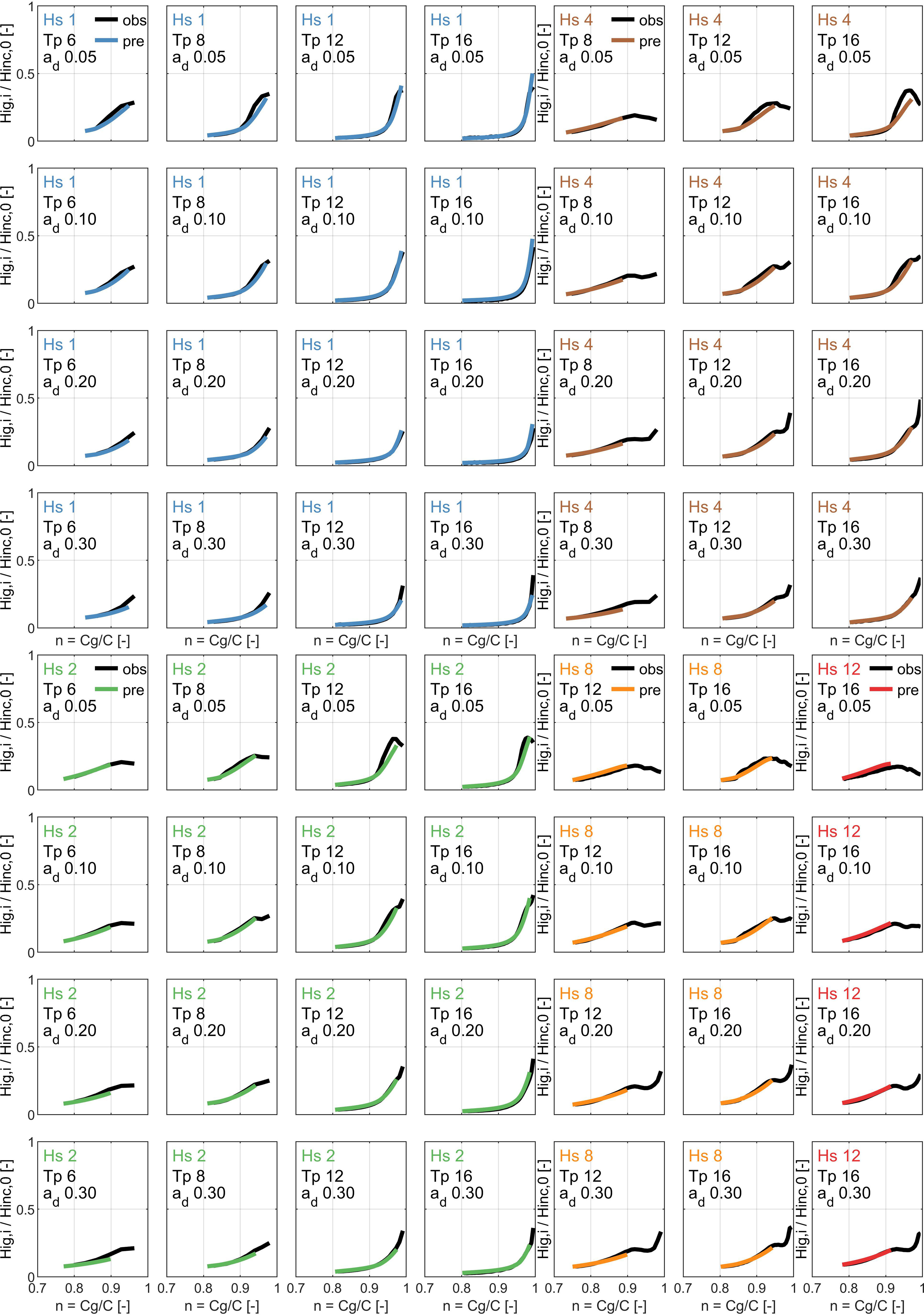
Figure A1 Observed (black) and predicted (colored) relative infragravity to offshore incident rms wave heights plotted against n (Cg/ C), for a range of offshore incident wave heights Hs [m] (shown in varying colors), peak wave periods Tp [s] and Dean slopes ad [-], all for beach slope 0.05.
Keywords: infragravity waves, nearshore wave conditions, wave modeling, computational efficiency, beaches, extreme events, flood risk
Citation: Leijnse TWB, van Ormondt M, van Dongeren A, Aerts JCJH and Muis S (2024) Estimating nearshore infragravity wave conditions at large spatial scales. Front. Mar. Sci. 11:1355095. doi: 10.3389/fmars.2024.1355095
Received: 13 December 2023; Accepted: 19 February 2024;
Published: 13 March 2024.
Edited by:
Jose A. Jimenez, Universitat Politecnica de Catalunya, SpainReviewed by:
Alec Torres-Freyermuth, Universidad Nacional Autónoma de México, MexicoLuigi Cavaleri, National Research Council (CNR), Italy
Copyright © 2024 Leijnse, van Ormondt, van Dongeren, Aerts and Muis. This is an open-access article distributed under the terms of the Creative Commons Attribution License (CC BY). The use, distribution or reproduction in other forums is permitted, provided the original author(s) and the copyright owner(s) are credited and that the original publication in this journal is cited, in accordance with accepted academic practice. No use, distribution or reproduction is permitted which does not comply with these terms.
*Correspondence: Tim W. B. Leijnse, VGltLkxlaWpuc2VAZGVsdGFyZXMubmw=