Application of coastal acoustic tomography: calibration of open boundary conditions on a numerical ocean model for tidal currents

Coastal acoustic tomography (CAT), which measures path-averaged currents from reciprocal acoustic transmission experiments and reconstructs velocity fields from the multiple path-averaged current data, is useful for monitoring tidal currents in coastal shallow water, especially if data assimilation is employed. Previous CAT data assimilation studies have focused on state estimation problems, i.e., the reconstruction of tidal currents and following dynamical discussion. In this study, we investigate the use of path-averaged currents in a boundary control problem. Specifically, we aim to use the observed path-averaged currents to determine the parameters of a numerical ocean model, which were tidal amplitudes and phases as the open boundary conditions in this study. We investigate two methods: using the ensemble Kalman filter (EnKF) results and a linearization approach called model Green’s function method. Both calibration methods decreased the amplitudes of tidal constituents at the open boundaries. We compare the model performance between the model predictions with and without the calibration of the open boundary conditions. The model predictions with the calibrated open boundary conditions improved the agreement with the observed path-averaged current. We also implemented the sequential updates of EnKF with the two calibrated open boundary conditions. The EnKF results with the independently calibrated two open boundary conditions improved the agreement with the comparison data obtained by acoustic Doppler current profiler measurement compared with the original EnKF result with the initial open boundary conditions.

1 Introduction

Sound waves are a practical tool for remotely sensing the ocean interior where the electromagnetic waves cannot penetrate and thus cannot be used as an observational tool. There are various applications that actively or passively use sound as a tool to know the ocean (or ocean-related issues), and those applications are termed acoustical oceanography (e.g., Howe et al., 2019). One such example of acoustical oceanography is using sound to infer the two- or three-dimensional fields of ocean sound speed and ocean currents (e.g., Worcester, 1977; Elisseeff et al., 1999; Dushaw et al., 2001, 2010). Sound travels faster through the warm (and high-salinity) water and with the direction of the ocean currents than through the cold (and less saline) water and against the ocean currents; thus, one can inversely estimate the sound speed and ocean currents by transmitting a sound pulse and measuring the travel time of the received pulse between multiple sources and receivers located horizontally separately. The effects of sound speed and current on the travel time can be separated by making transmissions in the forward and reverse directions between a pair of transceivers, namely a reciprocal transmission. The sound speed is related to the sum of the travel times of a reciprocal transmission, while the magnitude of ocean current is related to the differential travel times. Sound travels through the ocean at about 1,500 m s⁻¹, which is sufficiently fast compared with the timescales of ocean mesoscale eddies and the speed of observation vessels. Thus, this acoustical method is unique in the sense that one can estimate the nearly instantaneous state of the ocean interior. The method is known as ocean acoustic tomography (OAT; Munk and Wunsch, 1979; Munk et al., 1995). It is often referred to as acoustic thermometry (Dushaw et al., 2009) or coastal acoustic tomography (CAT; Kaneko et al., 2020) when the method is specially used to study large-scale ocean temperature estimation or dynamics of coastal shallow waters with relatively small spatial scales. This paper is closely related to CAT, and we focus on the method as a reconstruction tool of tidal currents in coastal shallow water.

Reconstructing velocity fields of tidal currents from observed travel times corresponds to solving an inverse problem. In CAT inverse problems, it is often the case that there is no unique solution (namely, the problem is ill-posed). Previous studies have solved their inverse problems and found solutions using some prior knowledge or regularization methods (e.g., Yamaoka et al., 2002; Yamaguchi et al., 2005). Researchers have tried to improve the estimations in such ill-posed problems by deploying a relatively large number of transceivers (Zhang et al., 2017a), by distributing transceivers to form a sensor network (Huang et al., 2013; Zhang et al., 2017b), or by using ships or autonomous vehicles to augment the travel time observation on various paths (Huang et al., 2019). Another promising approach for sparse observation (compared with a dimension of states) is data assimilation. In data assimilation, predictions from dynamical models (numerically modeled Navier-Stokes equations, for example) are optimally combined with observation data (e.g., Carrassi et al., 2018). Several CAT studies have implemented the ensemble Kalman filter (EnKF; Evensen, 1994, 2003) as a data assimilation scheme. These CAT data assimilation with EnKF have improved reconstruction compared to the results obtained by solving data-oriented inverse problems (e.g., Park and Kaneko, 2000; Lin et al., 2005; Zhu et al., 2017). The authors also demonstrated the usefulness of CAT data assimilation; strong and rapid spatiotemporal variation in the tidal current, including an island wake with multiple vortex generation at a downstream side of an island, was reconstructed by a CAT data assimilation with EnKF scheme (Taniguchi et al., 2023). As described here, previous CAT studies have mainly focused on reconstructing velocity fields of tidal currents; these may be termed state estimation problems (Munk et al., 1995).

In this study, as opposed to the previous CAT studies for state estimation problems, we investigate the use of reciprocal acoustic transmission data to ask what open boundary conditions are required to drive the ocean model so that it reproduces the sequence of observed states. Such a problem may be referred to as a boundary control problem (Munk et al., 1995) in contrast to the state estimation problem. Specifically, using the observation data and the numerical model used in the previous report (Taniguchi et al., 2023), we control (or calibrate or optimize) the parameters of the open boundary condition, which were tidal amplitudes and phases and determined in a somewhat ad-hoc way, by using the observed path-averaged currents. Since open boundary conditions can affect the states throughout the model domain while path-averaged currents obtained by reciprocal acoustic transmission contain the non-local information averaged over the paths, it is expected that path-averaged currents can effectively be used to control open boundary conditions. For this purpose, we investigate two methods: the use of EnKF results and a linearization approach proposed by Menemenlis et al. (2005). In the first method, data assimilation with the EnKF scheme can sequentially update the velocity fields of tidal currents as with the previous report (Taniguchi et al., 2023); then, we apply a harmonic analysis to the time series of normal velocities at open boundary grids and re-compute the amplitudes and phases of tidal constituents there. The second method is termed model green’s function approach in Menemenlis et al. (2005). The method assumes that the differences between the observed values and model-predicted values with initial model parameters can be represented by a linear combination of the sensitivity of model predictions to those model parameters. With the assumption, the practical method involves the numerical experiments of model sensitivity to the parameters followed by solving a linear inverse problem to find how much one should deviate the model parameters from the initial values. The method has been used widely as the parameter optimization method in many studies, including tide-related studies with local and regional scales (e.g., Moon et al., 2012; Kobayashi et al., 2016). We compare the model prediction accuracy between the models with and without the calibration of the open boundary conditions. Also, with the calibrated tidal parameters determined by the two methods, we re-perform the sequential data assimilation with EnKF to estimate the velocity fields at each transmission time. We shall show that both EnKF results with the independently calibrated two open boundary conditions improve the agreement with the acoustic Doppler current profiler observations compared to the original EnKF results with uncertain open boundary conditions.

2 Materials and methods

2.1 Field experiment

An experiment on reciprocal acoustic transmission between four acoustic stations was conducted in an area named Mihara-Seto in the Seto Inland Sea, Japan, from the end of October to December 2020. Figure 1 shows the geographical location of the observation site and the locations of the four acoustic stations named S1, S2, S3, and S4. The coast blocks the transmission between the S1 and S4 stations, i.e., the travel time between them is not observable. During the first two weeks of the experiment, the reciprocal transmissions between the S2 and S3 stations failed almost every low tide, which might be due to the existence of shallow sand banks near the S3 station. Two weeks after the experiment started, we slightly moved the location of S3 to prevent the sound propagation block by the shallow bank. The distances between the five station pairs (S1 and S2, S1 and S3, S2 and S3, S2 and S4, and S3 and S4) were 2,842, 4,930, 2,895, 4,300, and 4,220 m, respectively, after the S3 location was moved.

Figure 1

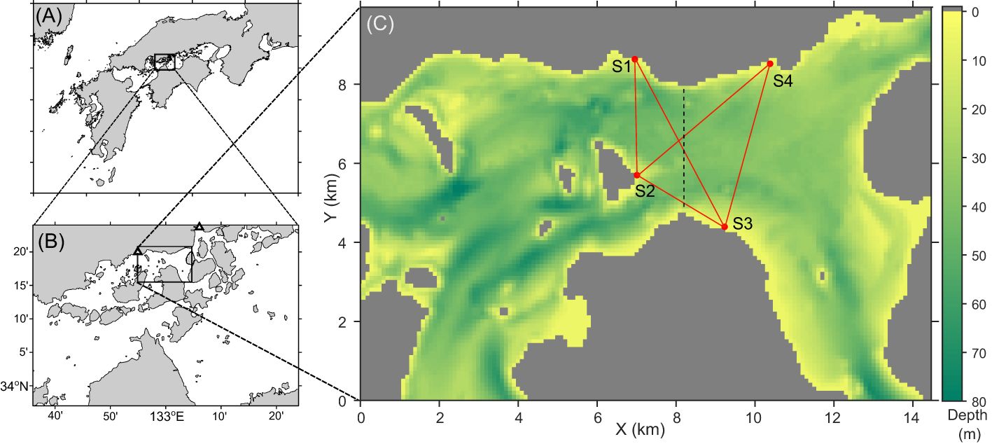
Figure 1 (A, B) Geographical location of observation site (Mihara-Seto) in the Seto Inland Sea, Japan; (C) domain of a numerical ocean model used in this study with the corresponding locations of acoustic stations (four red circles with labels S1, S2, S3, and S4) while the color indicates the water depth. The two black triangles in panel (B) is the location where astronomical tide information is obtained: Takehara for the west and Itozaki for the east. In panel (C), the black dashed line indicates the tracks of shipboard acoustic Doppler current profiling (ADCP) observation performed on Oct. 30. The ADCP observation was also performed nearly along the transmission paths (red solid lines) on Oct. 31 except for the path between the S2 and S3 stations.

The acoustic transmitting/receiving system used for this travel time measurement was a further modified version of the system used in a preliminary experiment in the same area in 2019 (Taniguchi et al., 2021a), which was a modification of the system originally used in a moving ship tomography study (Huang et al., 2019). The system consisted of three primary items: a microcontroller with peripheral electrical circuits, a global navigation satellite system (GNSS) receiver module and antenna, and an electro-acoustic transducer. The electro-acoustic transducer used in this experiment was the Model T235 of Neptune Sonar, which can operate over a frequency range of 10–25 kHz, and was used as a transceiver (i.e., both transmitter and hydrophone). The deployments of the transceivers were the same as those in the preliminary experiment (Taniguchi et al., 2021a). The sound transmission circuit consisted of a full-bridge inverter and a step-up voltage transformer. The amplified signal was fed to the transducer with an additional tuning inductor. The source level at full resonance was estimated to be 190 dB re 1 µPa at 1 m. The received signals were amplified and demodulated into in-phase and quadrature components. These two signals were digitized by a 12-bit analog-to-digital converter in the microcontroller. The sampling frequency was twice the carrier frequency of the transmitted signal. The digitized data were then recorded on an SD memory card on the electrical circuit board.

A pulse compression method has been implemented to increase the signal-to-noise ratio (SNR) without sacrificing the time resolution. The transmission signal was a binary phase-shift keyed signal encoded by a pseudo-random binary sequence called a maximal length sequence, which is often referred to as an m-sequence, with a carrier frequency of 18.018 kHz. The length of the m-sequences was 2,047 digits, and each digit contained four carrier cycles. The last 63 and the first 64 digits of the m-sequence were added to the head and tail of the m-sequence, respectively, to achieve the original autocorrelation property of repeated m-sequences during the matched filtering operation (Taniguchi et al., 2021b). The duration of the transmitted signal was then 482 ms. The four stations transmitted the signal in synchronization with the GNSS timing pulse, but with fixed time lags given to each station so that the arrival signals of other stations did not overlap at all stations (Taniguchi et al., 2021b). At the receiver side, the arrival signal appeared as sharp arrival pulses after calculating the cross-correlation between the received (demodulated) signal and the replica of the transmitted m-sequence. A post processing gain of this matched-filtering was 33 dB. Such reciprocal transmissions were performed every two minutes. More information on the system and signal for the reciprocal acoustic transmission experiment can be found in the authors’ previous papers (Taniguchi et al., 2021a, 2021b, 2023).

In the shallow water environment of the observation site, acoustic waves propagating along multiple ray paths arrive at the receiver nearly simultaneously, forming an arrival pulse that is slightly wider than the pulse width of a single ray arrival (Taniguchi et al., 2021a). In such cases, it is difficult to determine the arrival time of individual rays. Thus, the time at which the height of the received arrival pattern first exceeded 14 dB was adopted as the travel time in this study. By adopting such a relatively low threshold, we aimed to capture the arrival time associated with the first arrival, which would be composed of the arrivals of direct and surface-reflected rays (Taniguchi et al., 2021a). We confirmed that 14 dB is generally higher than the noise level and captures the rising edge of the first arrival pulses.

For each paired reciprocal acoustic transmission, differential travel times (τ_d) were computed from the determined travel times and converted to path-averaged current (u) as follows (Worcester, 1977; Howe et al., 1987; Zheng et al., 1997):

$\begin{array}{ll}u=-\frac{c_0^2}{2L}{\tau }_{\text{d}},& (1)\end{array}$

where L is the transceiver-to-transceiver distance, and c₀ is the reference sound speed value estimated using the sum of the reciprocal travel times. In this study, we computed the τ_d as, for example, τ_d = τ_S1←S2 − τ_S2←S1, i.e., the travel times of sound pulses from the station with a larger id to the station with a smaller id minus those from a smaller id to a larger id. In this case, with the minus sign in Equation 1, a positive value of u indicates that the direction of the path-averaged current is from the station with a larger id to the station with a smaller id. The erroneous estimates of the path-averaged velocity were removed and linearly interpolated if the data gaps were less than 10 minutes.

The water is well mixed in the sea around the observation site, and there is no density stratification. This condition allows the tidal currents to be nearly vertically uniform at the observation site. The vertically uniform velocity structure was also confirmed using the ADCP observation results (Taniguchi et al., 2021a). Therefore, the path-averaged currents determined from detecting the first arrival can be identified as the depth- and range-averaged currents. The above method of travel time determination made the path-averaged currents consistent with the acoustic Doppler current profiler (ADCP) results, as seen in the Results section.

Hourly shipboard ADCP observations were performed on October 30 and 31 to obtain velocity data for comparison with model and data assimilation results. Readers can refer to Taniguchi et al. (2023) for the ADCP operation parameters. Twenty-one cross-sections of velocity data were obtained along the north-south transect (black dashed in Figure 1) and along the transmission lines (red solid lines in Figure 1) from these ADCP observations. The obtained ADCP velocities were averaged over the depths at each location and also spatially (horizontally) averaged over about 100 m so that the spatial resolution of the ADCP velocity data is nearly the same as that of a numerical ocean model.

2.2 Numerical ocean model

A numerical ocean model used in this study was the same as that used in the authors’ previous study (Taniguchi et al., 2023) and was based on shallow water equations for the depth-averaged two-dimensional flows. The prognostic variables are eastward and northward components of the depth-averaged velocity (U and V) and tidal height, which is defined as a sea-surface height with respect to a mean sea level. The model domain with a horizontal grid space of 100 m is shown in Figure 1. The shallow water equations are solved numerically using the finite difference method with the numerical discretization and integration schemes following those used in the Princeton Ocean Model (POM; Blumberg and Mellor, 1987). The time integration with a time step of 1 s was performed using a leap-frog scheme with a Robert-Asselin filter with an additional modification proposed by Williams (2009).

The present model has six open boundaries (two at the west, east, and south), where prescribed tidal forcing (sea surface elevation and normal velocity) drives the model interior. The same boundary conditions were given to the two open boundaries at the west or east; thus, four open boundary conditions drove the model interior. A Flather condition is applied to the tidal height and normal velocity at the four open boundaries, following the form shown by Carter and Merrifield (2007). The tangential velocities at the boundary grids were given by the values of neighboring interior grids (i.e., a zero-gradient condition).

The normal velocity v and tidal height ζ at the open boundary grids were given by the sum of variation due to five tidal constituents:

$\begin{array}{ll}v(t)={\displaystyle \sum _{i=1}^5{A}_i\cos }\left(\frac{2\pi t}{T_i}+{\theta }_i\right),& (2)\end{array}$

$\begin{array}{ll}\zeta (t)={\displaystyle \sum _{i=1}^5{B}_i\cos }\left(\frac{2\pi t}{T_i}+{\varphi }_i\right),& (3)\end{array}$

where A_i (B_i), T_i, and θ_i (ϕ_i) are the amplitude, period, and phase of the five tidal constituents, respectively. Note that T_i is known value for each tidal constituent. The five tidal constituents are M₂, S₂, N₂, K₁, and O₁ tides in this study. These five constituents are the five largest constituents in the Seto Inland Sea, including the observation site. The following three largest contributions are from the S_a, K₂, and P₁ tides. Since it requires observations with periods of about half or one year to separate the contribution of these tides from other tides by a harmonic analysis (the Rayleigh criterion; e.g., Schureman, 1958), we did not consider these tides because of the shorter duration of our travel time measurement. The forms of Equations 2, 3 are also expressed in the exchangeable forms of Equations 4, 5:

$\begin{array}{ll}v(t)={\displaystyle \sum _{i=1}^5}\left[a_i\cos \left(\frac{2\pi t}{T_i}\right)+b_i\sin \left(\frac{2\pi t}{T_i}\right)\right],& (4)\end{array}$

$\begin{array}{ll}\zeta (t)={\displaystyle \sum _{i=1}^5}\left[c_i\cos \left(\frac{2\pi t}{T_i}\right)+d_i\sin \left(\frac{2\pi t}{T_i}\right)\right].& (5)\end{array}$

The prescribed tidal heights ζ(t) at the west and east boundaries were derived from astronomical tides at the nearest tide stations: Takehara for the west and Itozaki for the east (triangles in Figure 1B). There is no tide station near the two southern boundaries. Thus, the tidal elevations at the southwestern and southeastern boundaries were given by the same tidal heights as the western and eastern boundaries.

Because there is no information on normal velocities at the open boundaries, these were determined via an ad-hoc way with the information on the observed path-averaged current as follows. We applied a harmonic analysis to the observed path-averaged current between the S1 and S3 stations and estimated the amplitudes and phases of each tidal constituent. We considered the estimated phases as representative phases for tidal currents at the observation site. Next, we computed the phase differences between the astronomical tides (for the tidal height) and the path-averaged currents for each constituent. Then, we shifted the phases of the path-averaged current by the estimated phase differences and set them to the phases for the normal velocity. As for the amplitudes, we obtained the maximum tidal current at the center of the channel located at the northeastern boundary as about 2.8 m s⁻¹ from a nautical chart (not shown here). This maximum current speed was multiplied by 0.8 to roughly convert it to section-averaged current speed, resulting in a maximum section-averaged current of 2.2 m s⁻¹. Here, the relationship between the maximum and the section-averaged flow with coefficient 0.8 was derived by referring to those relationships in turbulent pipe flow with the one-seventh power low. Then, the amplitudes of the estimated five tidal constituents of the path-averaged current were scaled so that the reconstructed tidal currents by the five constituents reached 2.2 m s⁻¹ at the maximum during a spring tide. We set these scaled amplitudes as the amplitudes for the normal velocity at the northeastern boundary. Then, amplitudes of the five constituents at other western and southern boundaries were determined so that the volume transport through these boundaries without the tidal heights equaled that at the northeastern boundary. As described here, the open boundary conditions were derived arbitrarily, particularly for the normal velocity. Therefore, controlling (calibrating) those boundary conditions is expected to improve the reconstruction of tidal currents.

2.3 Open boundary condition improvement

2.3.1 Ensemble method

In the previous report (Taniguchi et al., 2023), we demonstrated that data assimilation with EnKF improves the reconstruction of tidal currents compared with the model prediction without data assimilation. The calibration of the open boundary conditions uses the results of the data assimilation with EnKF. Specifically, by applying harmonic analysis to the time series of velocity fields obtained by the data assimilation with EnKF, we re-compute the amplitudes and phases of tidal constituents at the open boundary grids. We focus on a relatively narrow area in the present study (see Figure 1). In such a narrow area, tidal currents are spatially correlated throughout the model domain, and thus, ensemble correlation in the covariance can be used as the physical (or real) correlation between the states. The velocity at the open boundaries would have been reasonably updated by EnKF via those physical correlations, even though the open boundaries are somewhat apart from the transmission paths. Thus, applying harmonic analysis to the results of EnKF data assimilation, one can determine better amplitudes and phases of the tidal constituents.

The EnKF implementation is nearly identical to that in the previous paper (Taniguchi et al., 2023). Readers can refer to Taniguchi et al. (2023) for the EnKF implementation specific to the present study. Below, we describe some key features. Ensembles of 98 members are created by perturbing the amplitudes and phases of the forcing tidal height and normal velocity at the open boundary girds; this method, i.e., perturbing boundary condition by adding noise to each ensemble, is commonly used in CAT data assimilation with EnKF. The model integration started at 00:00 on October 25, 2020, with no motion as the initial condition. The data assimilation step (EnKF updates) started at 16:00 on October 28, which is the approximate time when the path-averaged currents for all the station pairs started to be measured. The model state update was repeated every two minutes. If the number of successful reciprocal transmissions was two or less, the EnKF update was skipped at that time. The state vector contains the east-west and north-south velocity components (U and V) and tidal height at all grids. Both the velocities and tidal height were updated, although the tidal height was not observed in the reciprocal acoustic transmission experiment. The covariance localization was not implemented because the state vector must be updated throughout the model domain, including the open boundary grids. The covariance inflation was implemented with an inflation factor of 1.02.

A difference from the previous implementation was the value of observation error covariance, which is used to make perturbed measurements (Burgers et al., 1998) and to compute the data error covariance matrix in Kalman gain. During the investigation, we found that specifying small observation errors (e.g., 0.025 m s⁻¹; Taniguchi et al., 2021a) led to implausible updates of the state vector and spurious variation apart from the observations sometimes. The value of the observation error 0.025 m s⁻¹ was obtained as a time-averaged value on the S1S2 path (Taniguchi et al., 2021a), and this value was likely to underestimate the observation error for some specific periods. Thus, after some trial and error, we set the observation error to 0.05 m s⁻¹ (0.05² m² s⁻² in a variance), twice the value we obtained as the time-averaged path-averaged current precision. Additional consideration was given to the data error covariance. The present model aimed to reproduce relatively large tidal vortices that are found in the Seto Inland Sea (e.g., Arai, 2004), and it can simulate the generation of an island wake with a size of about 1 km (Taniguchi et al., 2023). By contrast, the observed path-averaged currents may contain contributions from smaller spatial scale features. Thus, there may be representation errors between the numerical model and the observed path-averaged currents. In the presence of representation errors, spurious variations will appear in the model prediction if the model is tightly fitted to the observed data. After some trial and error, we further reduced the impact of the observations by adding a diagonal matrix with a value of 0.08² m² s⁻² to the observational error covariance matrix in the Kalman gain. The added noise was somewhat large, but the EnKF updates keep the model state close to the observed path-averaged currents because of frequent updates of two minutes.

The EnKF updates were continually performed for 30 days. The data for 30 days were used in the harmonic analysis because the separation between M₂ and N₂ constituents needs nearly 30 days (Rayleigh criterion; e.g., Schureman, 1958). The updated tidal heights and normal velocities at the open boundary grids were averaged along the boundary and stacked for 30 days. Then, the harmonic analysis was applied to these time series at each open boundary to determine the amplitudes and phases of five tidal constituents (A_i, B_i, θ_i, ϕ_i); and these obtained amplitudes and phases of the tidal constituents provide the new open boundary conditions. Note that, in the narrow model domain of the present model, the tidal currents have a physical correlation throughout the model domain. Thus, the EnKF can reasonably update the U or V values, although they can easily recover to the values specified as the boundary forcing.

2.3.2 Linearization method

Menemenlis et al. (2005) proposed a method for adjusting control parameters used in a general circulation model by using the results of model parameter sensitivity experiments. The method linearizes an ocean model prediction about a particular model trajectory and was named model Green’s function approach following a similar linearization method used in Menemenlis and Wunsch (1997), where model Green’s function was defined as the response of a general circulation model to unit perturbations of their state vector. Implementing the method is easy because we only need to repeat a model simulation to determine the model sensitivity to the control parameters. With the results of the sensitivity experiments, the problem is linearized and eventually reduced to solving a linear inverse problem. Following their method, we calibrate the open boundary condition, i.e., tidal amplitudes and phases of the normal velocities at the open boundaries.

In order to apply the method to our present study, we consider the results of harmonic analysis applied to the time series of the observed five path-averaged currents for 30 days as the observation data. Thus, the observation vector y contains the amplitudes and phases (equivalently, the coefficients a and b in Equation 4) of the five tidal constituents for the five paths of the reciprocal transmission as follows:

$\begin{array}{ll}{\mathit{\text{y}}}^T=\left[a_{{\text{M}}_2}^{\text{S}1\text{S}2},b_{{\text{M}}_2}^{\text{S}1\text{S}2},a_{{\text{S}}_2}^{\text{S}1\text{S}2},b_{{\text{S}}_2}^{\text{S}1\text{S}2},\cdots ,a_{{\text{O}}_1}^{\text{S}3\text{S}4},b_{{\text{O}}_1}^{\text{S}3\text{S}4}\right],& (6)\end{array}$

where we use boldface to represent vector variables as column vectors, and the superscript T indicates the transpose of a matrix (vector); the superscript characters on the right-hand side of Equation 6 indicate the station pairs for the reciprocal transmission experiment.

Observation equivalents must be predicted from the numerical ocean model. To do so, we express the time stepping of the numerical ocean model as

$\begin{array}{ll}\mathit{\text{x}}(t+\text{Δ}t)=\mathit{\text{M}}(\mathit{\text{x}}(t),\mathit{\text{η}}),& (7)\end{array}$

where x is the state vector and includes east-west and north-south components of the depth-averaged velocities at all model grids; Function M represents the one-step-ahead integration of our numerical ocean model; η is a model parameter vector. We consider the parameters in the boundary forcing as the model parameters; that is, η in Equation 7 contains a_i and b_i in Equation 4 for the five tidal constituents and at the four open boundaries:

$\begin{array}{ll}{\mathit{\text{η}}}^T=[a_{{\text{M}}_2}^{\text{W}},b_{{\text{M}}_2}^{\text{W}},a_{{\text{S}}_2}^{\text{W}},b_{{\text{S}}_2}^{\text{W}},\cdots ,a_{{\text{O}}_1}^{\text{SE}},b_{{\text{O}}_1}^{\text{SE}}],& (8)\end{array}$

where the superscript characters on the right-hand side indicate the locations of the open boundaries; for example, W and SE for west and southeast boundaries, respectively. Note that although there are other model parameters, such as a bottom drag coefficient and kinematic eddy viscosity coefficient, those are fixed in the present study, and we omit them from the model parameters and equations. To relate the outputs from the numerical ocean model with the observation vector y, we consider a vector accumulating the state vector at the transmission times (i.e., every two minutes) for 30 days as shown in Equation 9:

$\begin{array}{ll}{\mathit{z}}^T=[{\mathit{\text{x}}}_1^T,{\mathit{\text{x}}}_2^T,\cdots ,{\mathit{\text{x}}}_{21600}^T],& (9)\end{array}$

where the subscript indicates the index corresponding to the transmission time within 30 days. This accumulated state vector z and the above observation y are related by an observation equation:

$\begin{array}{ll}\mathit{\text{y}}=\mathit{\text{f}}(\mathit{z})+\mathit{\text{ϵ}},& (10)\end{array}$

where function f is a composite function corresponding to the operation that converts the model velocity fields to path-averaged currents and then derives the harmonic constants a_i and b_i for the five transmission paths. The residual vector is introduced to represent the error term between y and f(z). Since vector z depends solely on η provided that the same model is used and other parameters are fixed, Equation 10 can also be written in terms of model parameter vector η as follows:

$\begin{array}{ll}\mathit{\text{y}}=\mathit{\text{ɡ}}(\mathit{\text{η}})+\mathbf{\text{ϵ}},& (11)\end{array}$

where ɡ has a functionality similar to f but with a model run with parameters η.

Solving Equation 11 for η (or, finding η that minimizes ${\mathit{\text{ϵ}}}^T\mathit{\text{ϵ}}$) is a nonlinear inverse problem, but one can linearize ɡ(η). To linearize ɡ(η), we assume that optimal parameter values can be expressed as the sum of initial values (η₀) and control value (η_c). With the expression η = η₀ + η_c, we linearize ɡ(η) around η₀, and Equation 11 becomes:

$\begin{array}{ll}{\mathit{\text{y}}=\mathit{\text{ɡ}}({\mathit{\text{η}}}_0)+\frac{\partial \mathit{\text{ɡ}}}{\partial \mathit{\text{η}}}|}_{\mathit{\text{η}}={\mathit{\text{η}}}_0}{\mathit{\text{η}}}_{\text{c}}+{\mathit{\text{ϵ}}}^{\prime },& (12)\end{array}$

or, equivalently,

$\begin{array}{ll}{\mathit{\text{y}}}_{\text{d}}=\mathit{\text{G}}{\mathit{\text{η}}}_{\text{c}}+{\mathit{\text{ϵ}}}^{\prime },& (13)\end{array}$

where ${\mathit{\text{y}}}_{\text{d}}=\mathit{\text{y}}-\mathit{\text{ɡ}}({\mathit{\text{η}}}_0)$, and $\frac{\partial \mathit{\text{ɡ}}}{\partial \mathit{\text{η}}}{|}_{\mathit{\text{η}}={\mathit{\text{η}}}_0}$ in Equation 12 is replaced with matrix $\mathit{\text{G}}$. This matrix G is a sensitivity matrix formed by

$\begin{array}{ll}\mathit{\text{G}}=\left[\cdots ,\frac{\mathit{\text{ɡ}}({\mathit{\text{η}}}_0+k_j{\mathit{\text{e}}}_j)-\mathit{\text{ɡ}}({\mathit{\text{η}}}_0)}{k_j},\cdots \right],& (14)\end{array}$

where e_j is a unit vector, and thus k_je_j is a vector that has a value (k_j) only at j-th element and has 0 at other elements. Thus, constructing matrix G corresponds to evaluating the model sensitivity to each element of η.

By solving Eqiation 13, we obtain an estimate of the optimal η by η₀ + η_c. Assuming that η_c and ${\mathit{\text{ϵ}}}^{\prime }$ are modeled as Gaussian distributions with zero mean and covariance S and R, we seek η_c that minimizes the following cost function:

$\begin{array}{ll}J={({\mathit{\text{y}}}_{\text{d}}-\mathit{\text{G}}{\mathit{\text{η}}}_{\text{c}})}^T{\mathit{\text{R}}}^{-1}({\mathit{\text{y}}}_{\text{d}}-\mathit{\text{G}}{\mathit{\text{η}}}_{\text{c}})+{\mathit{\eta }}_{\text{c}}^T{S}^{-1}{\mathit{\text{η}}}_{\text{c}}.& (15)\end{array}$

The expected solution that minimizes $J$ of Equation 15 has the following analytical form:

$\begin{array}{ll}{\widehat{\mathit{\text{η}}}}_{\text{c}}={\left({\mathit{\text{G}}}^T{\mathit{\text{R}}}^{-1}\mathit{\text{G}}+{\mathit{\text{S}}}^{-1}\right)}^{-1}{\mathit{\text{G}}}^T{\mathit{\text{R}}}^{-1}{\mathit{\text{y}}}_{\text{d}},& (16)\end{array}$

which corresponds to that called Gauss-Markov estimates (Munk et al., 1995). Optimal tidal amplitudes and phases are then obtained as $\widehat{\mathit{\text{η}}}={\mathit{\text{η}}}_0+{\widehat{\mathit{\text{η}}}}_c$.

One needs to perform a series of sensitivity experiments to construct matrix G of Equation 14. Kobayashi et al. (2016) mentioned that the results of the sensitivity experiments were independent of the perturbation values in the sensitivity experiments. Yet, the perturbation in the sensitivity experiments should be large enough for the resulting perturbation to appear in the path-averaged currents. In the present study, the sensitivity experiments were performed with a constant value of k_j of +0.1 m s⁻¹ for all j (i.e., for all a and b in Equation 8). We confirmed that perturbing the coefficients (a and b) for the normal velocities by +0.1 m s⁻¹ caused the change in the harmonic analysis results of the resulting path-averaged currents in the sensitivity experiments.

When we compute the solution of Equation 16, the covariance R and S are required, but the values representing those in the true fields cannot be known precisely, and thus, we specified the values in R and S based on our estimate of the size of the elements in ${\mathit{\text{ϵ}}}^{\prime }$ and η_c. The number of data used in the harmonic analysis was 21,565, 21,576, 17,875, 21,138, and 21,159 for the S1S2, S1S3, S2S3, S2S4, and S3S4 pairs (paths), respectively. With such a sufficient number of data, the expected error variance of the least squares solution ($\widehat{a}$ and $\widehat{b}$ for all the paths) in the harmonic analysis was about 0.001² m² s⁻² assuming measurement noise in the path-averaged currents of 0.1 m s⁻¹. Although the accurate values in R were unknown, they were expected to be somewhat larger than 0.001² m² s⁻² because of other sources for ${\mathbf{\text{ϵ}}}^{\prime }$. In the present study, we then set R as a diagonal matrix with a value of 0.01² m² s⁻² for all the elements. Here, each element in ${\mathbf{\text{ϵ}}}^{\prime }$ was expected to have no correlation with each other. Our expectation for S was that the coefficients of tidal constituents with large amplitude (i.e., M₂ and S₂) would be more uncertain and specified by larger variances than those of the other constituents (N₂, K₁, and O₁). In the present study, we set S as a diagonal matrix with values of 0.05², 0.04², and 0.03² m² s⁻² for the elements associated with M₂, S₂, and other tidal constituents, respectively. The variances for the M₂ and S₂ constituents (0.05² and 0.04²) were about three and two times the variance of the other constituents (3 × 0.03² and 2 × 0.03²), respectively. After obtaining a solution, we confirmed that ${({\mathit{\text{y}}}_d-\mathit{\text{G}}\widehat{\mathit{\text{η}}})}^T({\mathit{\text{y}}}_d-\mathit{\text{G}}\widehat{\mathit{\text{η}}})$ was nearly equal to the trace of R (0.006 and 0.0055, respectively), and at the same time, the elements in $\widehat{\mathit{\text{η}}}$ were not unrealistic values and did not deviate extraordinarily from our expectations.

3 Results

Table 1 summarizes the initial and calibrated normal velocities as the open boundary condition: the amplitudes and phases of the five tidal constituents at the four open boundaries. The most apparent change is that the amplitudes after the calibration are smaller than those before the calibration for both calibration methods, particularly on the M₂ and S₂ constituents. For example, the M₂ amplitude at the eastern boundary had an initial value of 1.30 m s⁻¹, and when the boundary condition was calibrated by using the EnKF results and linearization method, the amplitudes decreased to 1.07 and 1.12 m s⁻¹ (i.e., about 18% and 14% reduction), respectively. The amplitude decreased at other boundaries, too. The decrease in the amplitudes is reasonable because the present ocean model would overly predict the velocity of tidal currents compared with ADCP observation (Taniguchi et al., 2023). The amplitude of the S₂ constituent also decreased after the boundary calibration. The ratio of M₂ and S₂ constituents ($A_{{\text{S}}_2}/A_{{\text{M}}_2}$), which related to the amplitude during the spring and neap tides, was 0.4 at the initial values and remained nearly the same after the calibration; but, slightly large variations are found in the results with the linearization method (0.38–0.46 for the four boundaries). The amplitudes of the N₂, K₁, and O₁ also decreased by the calibration in general. The phases of the tidal constituents are delayed by the calibration with the ensemble method, particularly at the west and southwest boundaries; for example, the phase of the M₂ constituent at the west boundary is 71 and 79 degrees before and after the calibration. As a result, the difference in the phases between the west (and southwest) and east (and southeast) becomes smaller in the calibration results with the ensemble method. On the other hand, there is no clear trend about the phase in the calibration results with the linearization method.

Table 1

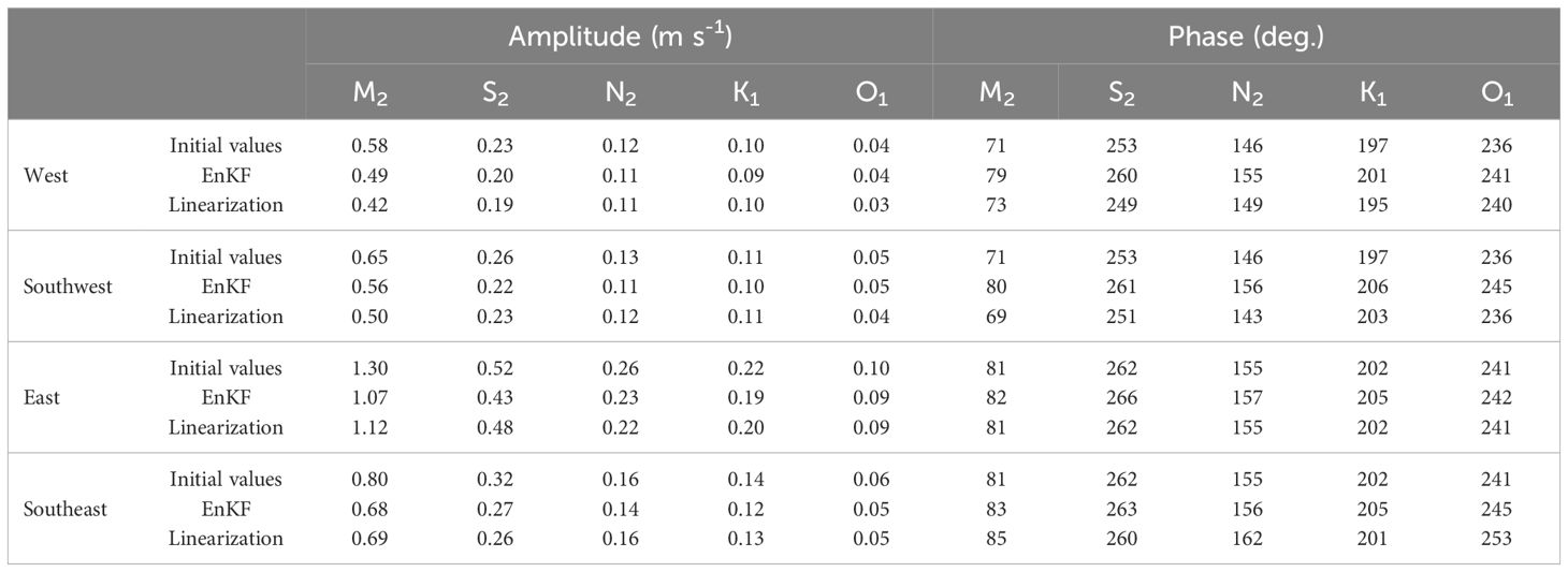
Table 1 Summary of the initial and calibrated boundary conditions (amplitude and phase).

We ran the numerical models with the calibrated open boundary conditions and predicted path-averaged currents. Figure 2 shows the results of harmonic analysis (reconstructed time series) applied to the observed and predicted path-averaged currents. The difference between the predicted and the observed path-averaged current decreased by the calibration of the open boundary condition (Figure 2B). Although the amplitude of the tidal constituents decreased by the boundary condition calibration, the amplitude of the observed path-averaged current is further small. When we compare the two methods, the linearization method resulted in the time series slightly closer to the observed results about the magnitude, which can be seen as the difference from the observed results (Figure 2B). The improvements by the boundary condition calibration are summarized in Table 2, which shows root-mean-squared differences (RMSD) between the observed and model-predicted path-averaged currents and their percent error relative to the observations. The improvements are mainly attained in the paths diagonally crossing the main course of the current (i.e., the S1-S3, S2-S3, and S3-S4 pairs). On the other hand, the improvements are minor for the paths crossing the main course at the right angle (the S1-S2 and S3-S4 pairs). Since the RMS magnitudes of the path-averaged currents for these paths are relatively small, the relative error remains large. Besides, there remains a clear phase error in the S3S4 path (Figure 2A5), while there is less phase error in other paths.

Figure 2

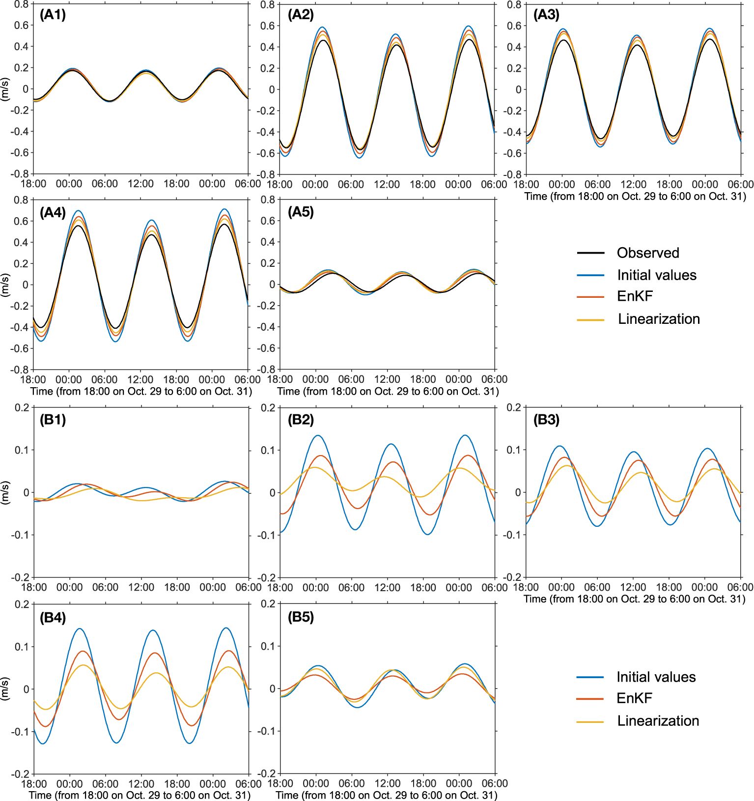
Figure 2 (A1–A5) Reconstructed path-averaged currents by using five taidal constituents (M₂, S₂, N₂, K₁, and O₁). The black line is from the observation and colored lines are model-predicted results: the blue, red, and yellow lines are the results with open boundary conditions of initial values, derived from EnKF results, and from linearization method, respectively. The five panels with label 1–5 correspond to the results of the S1-S2, S1-S3, S2-S3, S2-S4, and S3-S4 station pairs. (B1–B5) The difference of the model-predicted path-averaged currents (reconstructed by using five tidal constituents) with respect to the observed results. The line colors and panel’s label number are the same as those in (A1–A5).

Table 2

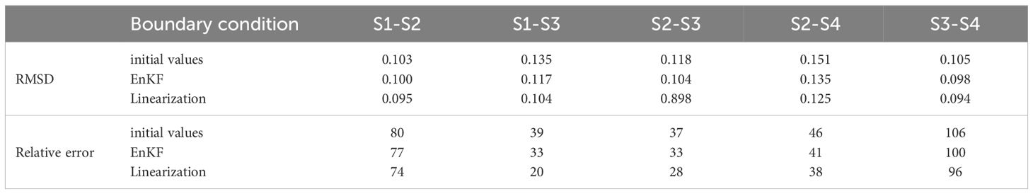
Table 2 Root-mean-squared differences (RMSD) between the model-predicted and the observed path-averaged currents for 30 days (m s⁻¹) and its relative error (%).

Figure 3A shows the observed and predicted path-averaged currents time series. The figure also shows the ADCP results (black thick lines), where the ADCP velocities were calculated by projecting the ADCP velocities at each observation point and averaging them over each transect. The observed path-averaged currents (gray solid lines) show high-frequency variation superimposed on sinusoidal variation. The path-averaged currents during the ADCP observations are consistent with the corresponding ADCP results. Thus, it is argued that the acoustic differential travel time signal captured the tidal current as a path-averaged quantity, and such high-frequency variations in the path-averaged currents indicate complex spatio-temporal features of the tidal currents.

Figure 3

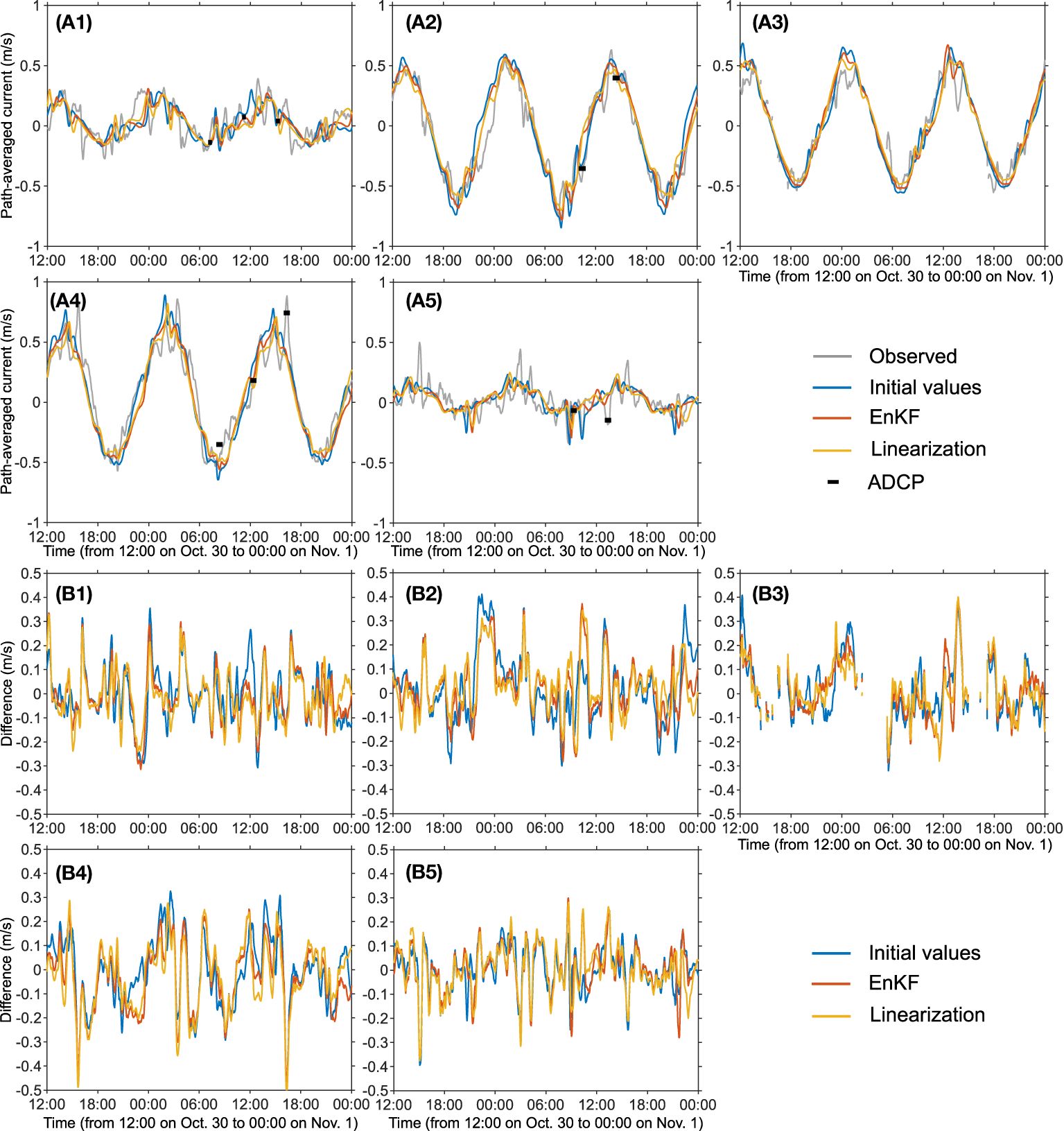
Figure 3 (A1–A5) Comparisons of the observed (gray) and model-predicted (colored) path-averaged currents. The blue, red, and yellow lines are the results with the open boundary conditions of initial values, derived from EnKF results, and from linearization method, respectively. The thick black bars are the ADCP results averaged over each transmission path. The five panels with label 1–5 correspond to the results of the S1-S2, S1-S3, S2-S3, S2-S4, and S3-S4 station pairs. (B1–B5) The difference of the model-predicted path-averaged currents with respect to the observed results. The line colors and panel’s label number are the same as those in (A1–A5).

The amplitude of the modeled path-averaged currents decreased because of the reduced tidal forcing (the normal velocity) at the open boundaries (Figure 3A). However, the high-frequency variation with periods of about 1–2 hours is not well reproduced, as shown in the plots of the difference between the modeled and observed path-averaged currents (Figure 3B). In particular, the magnitude of the high-frequency variation on the S3S4 path (Figure 3A5) is comparable to the tidal sinusoidal variation (with a period of the M₂ constituent); this may be one reason why a phase error appears on this path in the harmonic analysis result (Figure 2A5). Because the periods of the tidal constituents (e.g., about 12.4 hour for the M₂ constituent) are much longer than the periods of fluctuations in the model error (Figure 3B) or the high-frequency (short-period) variations in the path-averaged currents, calibration of the tidal boundary condition is not effective in improving the reproducibility of these high-frequency variations.

Figures 4, 5 show the comparisons of velocity vectors between the model predictions and ADCP observations in the form of spatial velocity fields and scatter plots, respectively. Table 3 summarizes the performance metrics of the comparisons: correlation coefficients and RMSD for the eastward and northward currents (r_U and r_V; RMSD_U and RMSD_V). We also computed fractional error variance (FEV) for the results with the initial and calibrated boundary conditions. The FEV is defined as

Figure 4

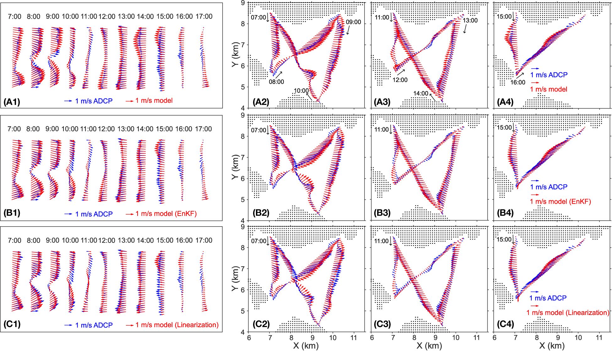
Figure 4 Comparisons of velocity vectors between the ADCP results (blue) and model-prediction (red). The model prediction results are obtained from the original boundary condition, the normal velocity calibrated by using the ensemble method, and those by using the linearization method from the top to the bottom, respectively. Panels (A1, B1, C1) are the comparisons with the ADCP results on Oct. 30, and panels (A2–A4, B2–B4, C2–C4) are the comparisons with the ADCP results on Oct. 31.

Figure 5

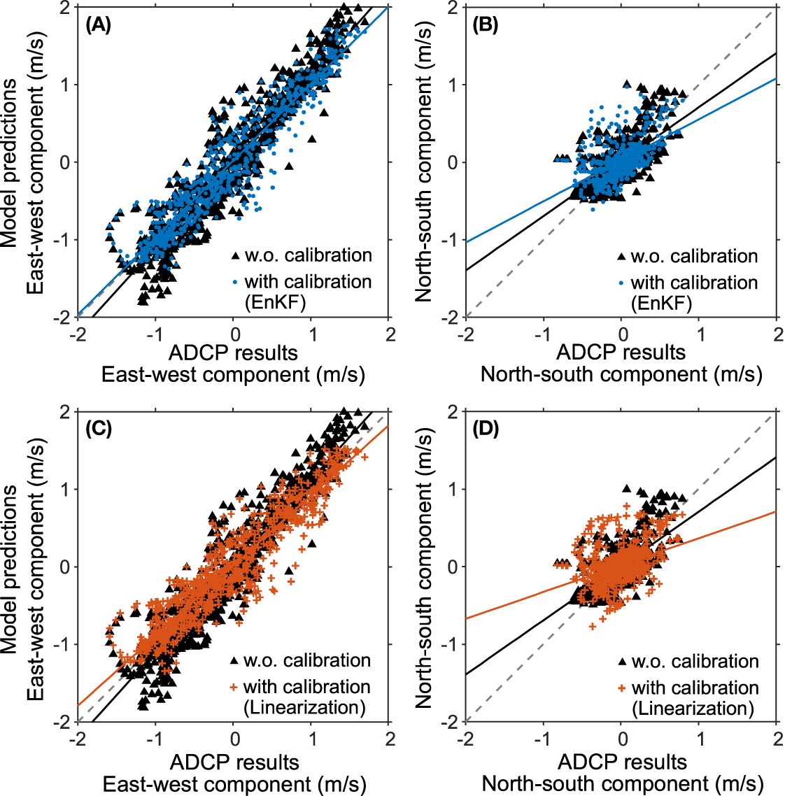
Figure 5 Scatter plots of ADCP observation results and model predictions without (black triangles) and with (colored) the calibration of open boundary condition (A, B) by applying a harmonic analysis to the EnKF results, and (C, D) by the linearization approach. In each panel, gray dashed line is the 1:1 line, and the solid lines indicate the linea regression lines.

Table 3

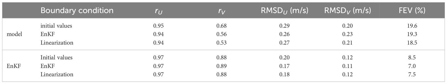
Table 3 Summary of the comparison with ADCP observed currents.

$\begin{array}{ll}\text{FEV}=\frac{\langle |U_i+j{V}_i-(U_i^{\text{ADCP}}+j{V}_i^{\text{ADCP}}){|}^2\rangle }{\langle |U_i^{\text{ADCP}}+j{V}_i^{\text{ADCP}}{|}^2\rangle },& (17)\end{array}$

where j × j = −1, and | · | and 〈 · 〉 indicate computing the absolute value and the averaging over the all ADCP data, respectively. Note that, for the comparisons with the ADCP results with Equation 17, the model results were spatiotemporally interpolated to obtain the velocity at the same locations and times as each ADCP velocity. In general, the model without the boundary condition calibration predicts the flow speed in the east-west component greater than that of the ADCP observations. This is evident in both the spatial velocity fields (Figure 4) and the scatter plots (the black triangles and corresponding regression lines in Figures 5A, C). The slope of the regression between the ADCP results and the model predictions without boundary calibration is 1.11 for the east-west component. The east-west components in the model prediction with the calibrated normal velocity are more compatible with the ADCP observations due to the reduced magnitude of the normal velocity at the open boundaries. With the calibrated boundary condition, the slopes became 0.99 and 0.90, for the ensemble and linearization methods, respectively. The linearization method decreased the slope a little too much. The RMSD_U decreased from 0.29 m s⁻¹ to 0.26 and 0.27 m s⁻¹ in the results of the boundary-calibrated model predictions (Table 3). In the spatial velocity map, the improvements are evident during the westward flow (transects starting at 13:00 and 14:00 on Oct. 30 and transects at 13:00, 14:00, and 15:00 on Oct. 31; Figure 4). Other examples of improvements in the spatial velocity map are found, for example, along transects starting at 8:00 and 9:00 on Oct. 30, although some degradation is also found (e.g., transects starting at 10:00 on Oct. 30 and 31).

Improvements in the north-south velocity component is not clear. The regression slopes became smaller in the boundary-calibrated model predictions than in the results without the calibrated boundary condition (Figures 5B, D). Also, the correlation coefficient decreased and RMSD increased (Table 3). Controlling the boundary condition to fit path-averaged currents does not minimize errors in east-west and north-south components independently. When the path-averaged currents are used as the data, the error in the east-west component mainly decreased because the contribution to the path-averaged currents from the east-west component is larger than those from the north-south component. Thus, the calibration does not always improve the north-south component of the velocity. However, it is true that the FEV (i.e., total error variance) is still decreased by the boundary condition calibration.

We evaluated if the boundary condition calibration affects sequential updates with EnKF by re-running EnKF updates with the calibrated boundary conditions. Although there were no distinguishable improvements in vector maps (like Figure 7 in Taniguchi et al., 2023), there were still some changes in EnKF results. Figure 6 exhibits the comparisons of velocity components between EnKF results and ADCP observations. For the eastward component of velocity, the EnKF results without the boundary calibration are still larger than the ADCP observations when the current magnitude is relatively large. This trend is found as that the EnKF results without the boundary condition calibration (black triangles) are higher than the identity line (1:1 line; black dashed line) at the first quadrant and lower than the 1:1 line at the third quadrant. The EnKF results with the new boundary condition (blue dots and red crosses in panels A and C) are more condensed around the 1:1 line than those without the boundary condition. The velocity magnitude of the northward component is small. Thus the difference between the EnKF results with and without the boundary calibration is not clear in the scatter plot. However, some outliers in the EnKF results without boundary calibration are well suppressed. Table 3 summarizes the comparisons of the EnKF results with ADCP observation. The EnKF results with the calibrated boundary condition improved its agreement with the ADCP observations. The RMSD for both eastward and northward components and for both the ensemble and linearization methods decreased. The FEV is 7.0% and 7.5% for the ensemble and linearization methods. These FEV values are smaller than the result obtained from the EnKF with 980 ensemble members in the previous report (FEV of 8.2%; Taniguchi et al., 2023).

Figure 6

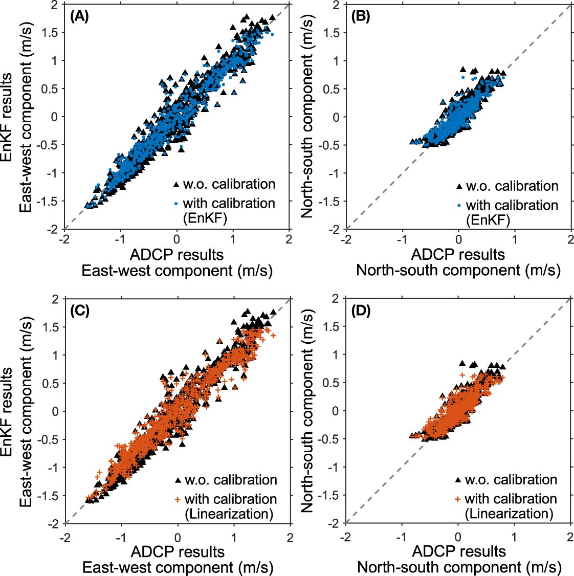
Figure 6 Scatter plots of ADCP observation results and EnKF results without (black triangles) and with (colored) the calibration of open boundary condition (A, B) by applying a harmonic analysis to EnKF results, and (C, D) by linearization approach.

Menemenlis et al. (2005) suggested that the parameter calibrations would be repeated to obtain better parameter values in strongly nonlinear conditions. We iterated the parameter calibration five times by re-computing the sensitivity matrix G in each iteration. Figure 7 shows the calibrated amplitudes of the M₂ constituent at the four boundaries over the iterations. Although the M₂ magnitude gradually changes and converges to some values, the largest change was at the first iteration. A similar trend was found in the magnitudes of the other constituents. In the EnKF for CAT, the boundary condition is perturbed to generate an ensemble, so relatively minor boundary modification after the first iteration might not affect the EnKF results. The FEV for the EnKF result with the boundary condition after the fifth iteration was 7.4, and there is not much additional improvement.

Figure 7

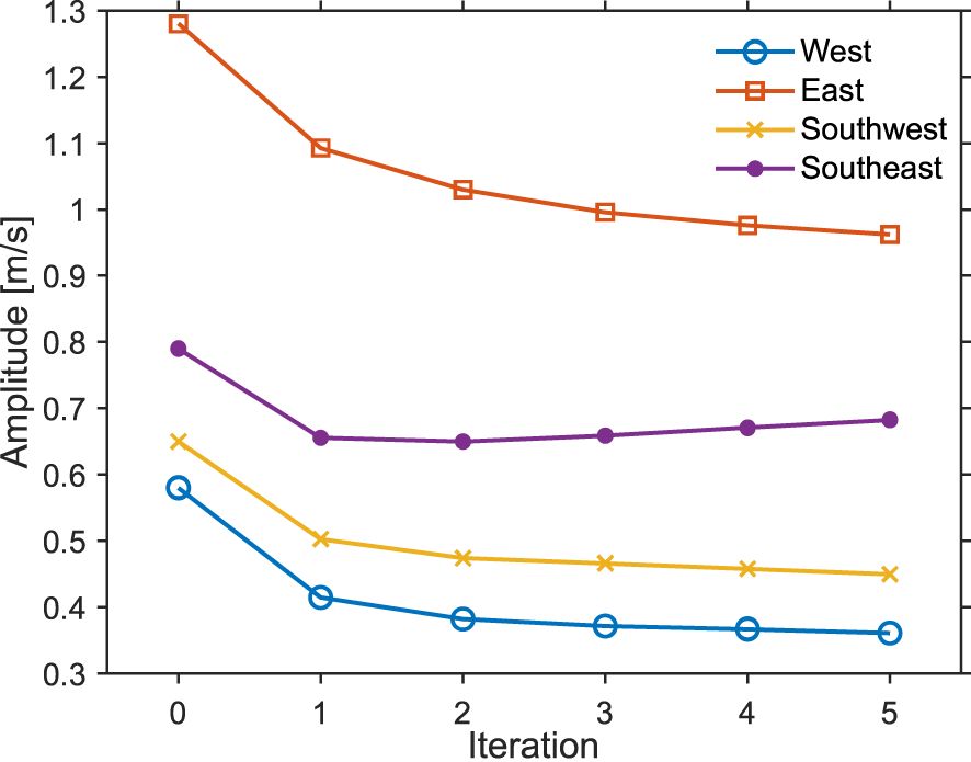
Figure 7 The variation of the M₂ amplitude for the normal velocity of the open boundary conditions on each iteration obtained by the linearization method. The values at the 0-th and first iterations correspond to those listed with labels Initial values and Linearization in Table 1.

4 Summary and discussion

In this paper, we demonstrated that the CAT path-averaged currents can also be used in a boundary control problem, i.e., to calibrate or tune the open boundary condition, which was the normal velocities at the open boundaries in this study. The two methods were able to derive nearly the same calibration results, particularly for the amplitude; both methods decreased the amplitudes of tidal constituents from the initial values. With the calibrated normal velocities, the agreement of the model-predicted velocity with the ADCP observations improved, although the improvements in the model prediction by the calibration were minor. A reason would be that the initial values of the normal velocities, which were ad-hocly determined using the observed path-averaged currents, were already reasonable to represent the major patterns of the tidal currents at the observation sites. Also, although we only used the velocity information and calibrated the normal velocities, the tidal height would have to be measured and calibrated as well as the normal velocities because the phase difference between the tidal current and height is one of the key factors controlling the velocity fields at the site. The EnKF data assimilation with the new boundary condition also improved the results in terms of the agreement with ADCP observations; in the EnFK results with the new boundary condition, the overestimated velocity magnitude, which was found in the EnKF results with the original boundary condition (Taniguchi et al., 2023) and due likely to the overly specified amplitude of the initial open boundary condition, decreased so that the agreement with ADCP results become better. Thus, the calibration of the boundary condition would be desired work, particularly when the boundary condition is uncertain. Related to the present study with the CAT, we are purposing developments of a real-time monitoring system of velocity fields of tidal currents. The practical implementation of the present method will be to perform the reciprocal acoustic transmission experiment first to calibrate the boundary condition, followed by the real-time monitoring with sequential assimilation with the calibrated model boundary condition.

Both two methods can control the tidal boundary condition. We do not provide the decision about which is better. The EnKF method is easier in terms of implementation because it performs sequential assimilation twice with the same computation code but with different boundary conditions. However, this method may limit the size of the model domain or target. The EnKF scheme updates the model states using the information on state covariance. Thus, if there is no correlation between the velocity fields at observation locations and at open boundaries, then the EnKF scheme cannot reasonably update the model states at open boundaries. Also, one may need to use relatively large ensemble members to suppress spurious correlation because the covariance localization, which reduces EnKF update impacts at grids far from the observation site, would be prohibited. The linearization method is not limited by the model size and can be used to adjust control parameters in a general circulation model (Menemenlis et al., 2005). However, if we include more constituents (over-tides and compound tides) as the target for the calibration, the necessary computation increases as the number of model parameters increases.

Areas of improvement remain. First, tidal height was not observed in the experiment; thus, the tidal height information was not used to calibrate boundary conditions and in the EnKF updates. The performance of the boundary condition calibration is expected to be improved by adding the tidal height observations. Or, one may observe the tidal height variations at open boundaries independent of reciprocal transmission experiment in order to determine the reliable amplitudes and phases of the tidal constituents at the open boundaries; in this case, one will focus only on updating velocity information by using the reciprocal transmission experiment data like that performed in this study. In the present model, the tidal elevations and normal velocities were constant along each open boundary. The model prediction may improve by specifying variable condition along the boundary and/or adding more constituents of overtides and compound tides for high frequency variation; however, controlling those additional parameters increases the computation when the linearlization method is employed. Also, controlling other model parameters, such as the coefficients for bottom drag and eddy viscosity, may contribute to further improvements.

The improvement of the EnKF results by the boundary condition calibration is slight (reduction of about 1% in FEV and 0.02–0.03 m s⁻¹ in RMSD_U and 0.01 m s⁻¹ in RMSD_V; Table 3). Figure 8 shows the ensemble spread σ for the east-west and north-south velocity components, computed immediately after the EnKF updates and averaged over two days of Oct. 30 and 31 (the days the ADCP observation was conducted). The ensemble spread σ is about 0.15 m s⁻¹ in the east-west component and about 0.1 m s⁻¹ in the north-south component in the tomography domain. The standard error of the ensemble mean is estimated as $\sigma /\sqrt{n}$, where n is the number of ensemble members, and the values are $0.15/\sqrt{98}\approx 0.015$ for the east-west component and $0.1/\sqrt{98}\approx 0.01$ for the north-south component. By comparing the RMSD improvements with these estimated standard errors of the mean, the improvement in the east-west component is expected to be statistically meaningful. By repeating the EnKF assimilation with the calibrated boundary conditions multiple times (with randomly generated ensemble members), we also confirmed that the resulting FEV and RMSDs changed slightly in each EnKF run; the EnKF results with the boundary calibration were consistently better (smaller FEV and RMSD_U). Although minor improvements do not contribute to the refinement of the instantaneous velocity fields of the tidal currents in a velocity map, it will be important when we focus on residual currents (or time-averaged flow), which are much smaller in magnitude compared to tidal currents and will be the subject when we start monitoring tidal currents operationally with EnKF-CAT.

Figure 8

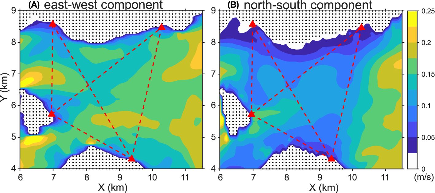
Figure 8 Posterior ensemble spread for (A) east-west and (B) north-south components. The results are obtained by executing the EnKF updates with the calibrated boundary condition (with the ensemble method). The results are averaged over two days on Oct. 30 and 31, the days when the ADCP observations were performed. The red triangles indicate the station locations and the red dashed lines are the acoustic transmission paths.

There is also room for improvement in CAT data assimilation. As shown by Cornuelle and Worcester (1996), path-averaged measurements (path-averaged currents in this study) determine the lower wavenumber information better than the higher wavenumbers, and determining the high wavenumber information requires a sufficiently small measurement error. The present EnKF implementation uses a relatively large data error covariance to suppress implausible EnKF updates. Thus, while the present EnKF reasonably determines the low wavenumber structure, it may lack the ability to determine the high wavenumber variation found in the ADCP observations. The need for a relatively large data error covariance may be due in part to representation errors. If the representation errors in a model are sufficiently small, then the data error covariance can only be given by the measurement noise in the path-averaged currents. Thus, more sophisticated numerical models are suitable for CAT data assimilation to fully exploit the information in the path-averaged currents. It will also be necessary to investigate how precise models are needed to effectively use the information in the path-averaged currents will also be required.

CAT with data assimilation is a promising tool for reconstructing the tidal velocity fields in coastal shallow water. However, there are still space for improving the CAT for the reconstructions of tidal currents. The present study is one such example. Since the velocity fields (and thus tidal currents) in coastal shallow water are essential information for various studies related to the ocean, improving the CAT performance to represent the ocean currents contributes to the progress of those fields.

Data availability statement

The data analyzed in this study is subject to the following licenses/restrictions: Data sets used in this study are the same as those used in the previous study (Taniguchi et al., 2023). Requests to access these datasets should be directed to ntaniguchi@hiroshima-u.ac.jp.

Author contributions

NT: Conceptualization, Formal analysis, Funding acquisition, Investigation, Methodology, Writing – original draft. HM: Conceptualization, Software, Writing – review & editing. MA: Methodology, Software, Writing – review & editing. YS: Funding acquisition, Resources, Writing – review & editing. KH: Methodology, Project administration, Resources, Writing – review & editing. C-FH: Conceptualization, Methodology, Writing – review & editing. JG: Conceptualization, Methodology, Writing – review & editing. TT: Data curation, Investigation, Resources, Writing – review & editing. KY: Data curation, Investigation, Resources, Writing – review & editing. HY: Data curation, Investigation, Resources, Writing – review & editing.

Funding

The author(s) declare financial support was received for the research, authorship, and/or publication of this article. This work was partly supported by JSPS KAKENHI Grant Numbers 19H04292, 20H02369, 20K14964, 22K04563.

Acknowledgments

The authors are grateful to Geinan Fisheries Cooperative Association, Mihara-Shi Fisheries Cooperative Association, Ohmishima (Ehime Prefecture) Fisheries Cooperative Association, and TSUNEISHI SHIPBUILDING Co., Ltd. for their support in the reciprocal acoustic transmission experiment.

Conflict of interest

Author TT, KY, and HY are employed by Fukken Co., LTD.

The remaining authors declare that the research was conducted in the absence of any commercial or financial relationships that could be construed as a potential conflict of interest.

Publisher’s note

All claims expressed in this article are solely those of the authors and do not necessarily represent those of their affiliated organizations, or those of the publisher, the editors and the reviewers. Any product that may be evaluated in this article, or claim that may be made by its manufacturer, is not guaranteed or endorsed by the publisher.

References

Arai M. (2004). Development of a semi-spectral coastal ocean model and its application to the neko seto sea in the seto inland sea. J. Oceanography 60, 597–611. doi: 10.1023/B:JOCE.0000038352.17595.4e

CrossRef Full Text | Google Scholar

Blumberg A. F., Mellor G. L. (1987). A Description of a Three-Dimensional Coastal Ocean Circulation Model (Washington, D.C.: American Geophysical Union (AGU), 1–16. doi: 10.1029/CO004p0001

CrossRef Full Text | Google Scholar

Burgers G., van Leeuwen P. J., Evensen G. (1998). Analysis scheme in the ensemble kalman filter. Monthly Weather Rev. 126, 1719–1724. doi: 10.1175/1520-0493(1998)126h1719:ASITEKi2.0.CO;2

CrossRef Full Text | Google Scholar

Carrassi A., Bocquet M., Bertino L., Evensen G. (2018). Data assimilation in the geosciences: An overview of methods, issues, and perspectives. WIREs Climate Change 9, e535. doi: 10.1002/wcc.535

CrossRef Full Text | Google Scholar

Carter G. S., Merrifield M. A. (2007). Open boundary conditions for regional tidal simulations. Ocean Model. 18, 194–209. doi: 10.1016/j.ocemod.2007.04.003

CrossRef Full Text | Google Scholar

Cornuelle B. D., Worcester P. F. (1996). “Ocean acoustic tomography: Integral data and ocean models,” in Modern Approaches to Data Assimilation in Ocean Modeling, vol. 61 . Ed. Malanotte-Rizzoli P. (Amsterdam: Elsevier Oceanography Series), 97–115. doi: 10.1016/S0422-9894(96)80007-9

CrossRef Full Text | Google Scholar

Dushaw B. D., Au W., Beszczynska-Moller A., Brainard R., Cornuelle B. D., Duda T., et al. (2010). “A global ocean acoustic observing network,” in Proceedings of OceanObs’09: Sustained Ocean Observations and Information for Society, vol. 2. (ESA Publication WPP-306). doi: 10.5270/OceanObs09.cwp.25

CrossRef Full Text | Google Scholar

Dushaw B. D., Bold G., Chiu C.-S., Colosi J. A., Cornuelle B. D., Desaubies Y., et al. (2001). “Observing the ocean in the 2000’s: A strategy for the role of acoustic tomography in ocean climate observation,” in Observing the Oceans in the 21st Century, Melbourne 391–418.

Google Scholar

Dushaw B. D., Worcester P. F., Munk W. H., Spindel R. C., Mercer J. A., Howe B. M., et al. (2009). A decade of acoustic thermometry in the North Pacific Ocean. J. Geophysical Research: Oceans 114. doi: 10.1029/2008JC005124

CrossRef Full Text | Google Scholar

Elisseeff P., Schmidt H., Johnson M., Herold D., Chapman N. R., McDonald M. M. (1999). Acoustic tomography of a coastal front in Haro Strait, British Columbia. J. Acoustical Soc. America 106, 169–184. doi: 10.1121/1.427046

CrossRef Full Text | Google Scholar

Evensen G. (1994). Sequential data assimilation with a nonlinear quasi-geostrophic model using Monte Carlo methods to forecast error statistics. J. Geophysical Research: Oceans 99, 10143–10162. doi: 10.1029/94JC00572

CrossRef Full Text | Google Scholar

Evensen G. (2003). The Ensemble Kalman Filter: theoretical formulation and practical implementation. Ocean Dynamics 53, 343–367. doi: 10.1007/s10236-003-0036-9

CrossRef Full Text | Google Scholar

Howe B. M., Miksis-Olds J., Rehm E., Sagen H., Worcester P. F., Haralabus G. (2019). Observing the oceans acoustically. Front. Mar. Sci. 6. doi: 10.3389/fmars.2019.00426

CrossRef Full Text | Google Scholar

Howe B. M., Worcester P. F., Spindel R. C. (1987). Ocean acoustic tomography: Mesoscale velocity. J. Geophysical Research: Oceans 92, 3785–3805. doi: 10.1029/JC092iC04p03785

CrossRef Full Text | Google Scholar

Huang C.-F., Li Y.-W., Taniguchi N. (2019). Mapping of ocean currents in shallow water using moving ship acoustic tomography. J. Acoustical Soc. America 145, 858–868. doi: 10.1121/1.5090496

CrossRef Full Text | Google Scholar

Huang C.-F., Yang T. C., Liu J.-Y., Schindall J. (2013). Acoustic mapping of ocean currents using networked distributed sensors. J. Acoustical Soc. America 134, 2090–2105. doi: 10.1121/1.4817835

CrossRef Full Text | Google Scholar

Kaneko A., Zhu X.-H., Lin J. (2020). Coastal Acoustic Tomography (Amsterdam: Elsevier). doi: 10.1016/C2018-0-04180-8

CrossRef Full Text | Google Scholar

Kobayashi S., Nakada S., Takagi S., Hirose N. (2016). Parameter optimization of a 3D coastal model using Green’s functions for modelling river plume dynamics. J. Advanced Simulation Sci. Eng. 3, 153–164. doi: 10.15748/jasse.3.153

CrossRef Full Text | Google Scholar

Lin J., Kaneko A., Gohda N., Yamaguchi K. (2005). Accurate imaging and prediction of Kanmon Strait tidal current structures by the coastal acoustic tomography data. Geophysical Res. Lett. 32. doi: 10.1029/2005GL022914

CrossRef Full Text | Google Scholar

Menemenlis D., Fukumori I., Lee T. (2005). Using green’s functions to calibrate an ocean general circulation model. Monthly Weather Rev. 133, 1224–1240. doi: 10.1175/MWR2912.1

CrossRef Full Text | Google Scholar

Menemenlis D., Wunsch C. (1997). Linearization of an oceanic general circulation model for data assimilation and climate studies. J. Atmospheric Oceanic Technol. 14, 1420–1443. doi: 10.1175/1520-0426(1997)014h1420:LOAOGCi2.0.CO;2

CrossRef Full Text | Google Scholar

Moon J.-H., Hirose N., Morimoto A. (2012). Green’s function approach for calibrating tides in a circulation model for the east asian marginal seas. J. Oceanography 68, 345–354. doi: 10.1007/s10872-011-0097-1

CrossRef Full Text | Google Scholar

Munk W., Worcester P., Wunsch C. (1995). Ocean Acoustic Tomography. Cambridge Monographs on Mechanics (New York: Cambridge University Press). doi: 10.1017/CBO9780511666926

CrossRef Full Text | Google Scholar

Munk W., Wunsch C. (1979). Ocean acoustic tomography: a scheme for large scale monitoring. Deep Sea Res. Part A. Oceanographic Res. Papers 26, 123–161. doi: 10.1016/0198-0149(79)90073-6

CrossRef Full Text | Google Scholar

Park J.-H., Kaneko A. (2000). Assimilation of coastal acoustic tomography data into a barotropic ocean model. Geophysical Res. Lett. 27, 3373–3376. doi: 10.1029/2000GL011600

CrossRef Full Text | Google Scholar

Schureman P. (1958). Manual of Harmonic Analysis and Prediction of Tides (Revised 1940 Edition Reprinted 1958 with correction). Special Publication No.98 (Washington D.C: Coast and Geodetic Survey, U.S. Department of Commerce).

Google Scholar

Taniguchi N., Mutsuda H., Arai M., Sakuno Y., Hamada K., Takahashi T., et al. (2023). Reconstruction of horizontal tidal current fields in a shallow water with model-oriented coastal acoustic tomography. Front. Mar. Sci. 10. doi: 10.3389/fmars.2023.1112592

CrossRef Full Text | Google Scholar

Taniguchi N., Takahashi T., Yoshiki K., Yamamoto H., Hanifa A. D., Sakuno Y., et al. (2021a). A reciprocal acoustic transmission experiment for precise observations of tidal currents in a shallow sea. Ocean Eng. 219, 108292. doi: 10.1016/j.oceaneng.2020.108292

CrossRef Full Text | Google Scholar

Taniguchi N., Takahashi T., Yoshiki K., Yamamoto H., Sugano T., Mutsuda H., et al. (2021b). Reciprocal acoustic transmission experiment at Mihara-Seto in the Seto Inland Sea, Japan. Acoustical Sci. Technol. 42, 290–293. doi: 10.1250/ast.42.290

CrossRef Full Text | Google Scholar

Williams P. D. (2009). A proposed modification to the robert–asselin time filter. Monthly Weather Rev. 137, 2538–2546. doi: 10.1175/2009MWR2724.1

CrossRef Full Text | Google Scholar

Worcester P. F. (1977). Reciprocal acoustic transmission in a midocean environment. J. Acoust. Soc Am. 62, 895–905. doi: 10.1121/1.381619

CrossRef Full Text | Google Scholar

Yamaguchi K., Lin J., Kaneko A., Yayamoto T., Gohda N., Nguyen H.-Q., et al. (2005). A continuous mapping of tidal current structures in the kanmon strait. J. Oceanogr. 61, 283–294. doi: 10.1007/s10872-005-0038-y

CrossRef Full Text | Google Scholar

Yamaoka H., Kaneko A., Park J.-H., Zheng H., Gohda N., Takano T., et al. (2002). Coastal acoustic tomography system and its field application. IEEE J. Ocean. Eng. 27, 283–295. doi: 10.1109/JOE.2002.1002483

CrossRef Full Text | Google Scholar

Zhang C., Zhu X.-H., Zhu Z.-N., Liu W., Zhang Z., Fan X., et al. (2017a). High-precision measurement of tidal current structures using coastal acoustic tomography. Estuarine Coast. Shelf Sci. 193, 12–24. doi: 10.1016/j.ecss.2017.05.014

CrossRef Full Text | Google Scholar

Zhang Y., Chen H., Xu W., Yang T. C., Huang J. (2017b). Spatiotemporal tracking of ocean current field with distributed acoustic sensor network. IEEE J. Oceanic Eng. 42, 681–696. doi: 10.1109/JOE.2016.2582018

CrossRef Full Text | Google Scholar

Zheng H., Gohda N., Noguchi H., Ito T., Yamaoka H., Tamura T., et al. (1997). Reciprocal sound transmission experiment for current measurement in the seto inland sea, Japan. J. Oceanogr 53, 117–127.

Google Scholar

Zhu Z.-N., Zhu X.-H., Guo X., Fan X., Zhang C. (2017). Assimilation of coastal acoustic tomography data using an unstructured triangular grid ocean model for water with complex coastlines and islands. J. Geophysical Research: Oceans 122, 7013–7030. doi: 10.1002/2017JC012715

CrossRef Full Text | Google Scholar