 Zhengrong Wei
 Yanliang Pei
 Xiangqian Zhu
 Kai Liu
 Xiaobo Zhang
 Le Zong
 Xinyu Li4
- 1College of Ocean Science and Engineering, Shandong University of Science and Technology, Qingdao, China
- 2First Institute of Oceanography of Ministry of Natural Resources, Qingdao, China
- 3Laboratory for Marine Geology, Qingdao Marine Science and Technology Center, Qingdao, China
- 4Key Laboratory of Deep Sea Mineral Resources Development, Shandong (Preparatory), Qingdao, China
- 5Key Laboratory of Submarine Acoustic Investigation and Application of Qingdao (Preparatory), Qingdao, China
Kuiyang-ST2000 is a deep-towed multichannel seismic system that provides high-resolution exploration of sub-seabed geological formations. Due to the uncertainty of the sound speed at full ocean depth, the travel-time positioning of sea surface reflected waves still has flaws in positioning arrays. This research reveals that the average sound speed of seawater selected for computing the array position only affects the vertical displacement of the arrays. thus, a polynomial fitting method is proposed to position the arrays. Because the nonuniform mass distribution complicates the array shape, first, the weight of the digital transmission unit is balanced by one designed floater so that the array shape becomes a simple convex curve during towing conditions. Afterward, one general sound speed is used to calculate the initial array position; then, the polynomial fitting method is used to tune the sound speed so that the seismic source and hydrophones are on the same convex curve. Finally, an accurate array position is calculated by the proposed positioning method, and the submarine shallow strata are imaged at a high resolution.
1 Introduction
The accuracy of array positioning is closely related to the data processing quality of deep-towed seismic exploration systems (Howard and Syck, 1992; Lu et al., 2003). Generally, vertical accuracy is required to reach a sampling interval (Δt), and horizontal accuracy is required to reach the 1/4 wavelength of the seismic wave (Krödel et al., 2015). However, the towing depth of deep-towed seismic systems is greater than 1000 m; therefore, navigation via a global positioning cannot be used to determine the geometric relationship between the source and the arrays. Additionally, due to the influences of retracting and releasing the towing cable, the instability of the towing speed and the variation in the deep-sea environment, the seismic source and arrays inevitably float up and down during the data acquisition process. Many researchers have focused on methods for aligning arrays (Varypaev and Kushnir, 2020; Nanni et al., 2022), positioning arrays (Vickery, 1998; Lan and Ding, 2012), and calibrating arrays (Fikes et al., 2019; Che et al., 2021).
The Deep Tow Array Geophysical System (DTAGS) is the first deep-towed multichannel seismic survey system developed by the Naval Ocean Research and Development Activity to measure the geoacoustic parameters of the ocean floor (Fagot et al., 1980; Chapman et al., 2002; Ker et al., 2010). The array positioning system of DTAGS relies mainly on depth sensors installed on towed vehicles and hydrophone 28 (at 138 m), hydrophone 38 (at 288 m) and hydrophone 48 (at 438 m) of the arrays. The water pressure and temperature are measured in a timely manner, and the values are converted to depth values according to an empirical formula for sea area measurements. Initially, the arrays between adjacent depth sensors are simplified as one straight line, and the position of each hydrophone in the arrays is calculated via linear interpolation (Rowe and Gettrust, 1993). However, this assumption does not conform to the real shape of the arrays, resulting in large errors in seismic data processing. These errors reduce the signal-to-noise ratio of the seismic data after stacking imaging. The travel time of a sea surface reflection (SSR) wave has been used to locate the arrays, improving the accuracy of the relative positions between the source and hydrophone in single-shot gathering (Walia and Hannay, 1999). The array shape calculated with depth sensors is simultaneously constrained by the travel time of direct waves and SSR waves, and the genetic algorithm can be used to optimize the sound speed by He (He et al., 2009). Although the positioning accuracy is improved, it is still unsatisfactory because the water depths measured by depth sensors have errors of 3-5 m. Following that, it was determined that direct waves and SSR waves can be picked up more accurately from waveform envelope lines (Kong et al., 2012). However, due to the time delay in data acquisition, direct wave signals can be measured only at the last 3~4 hydrophones, and the positioning of the front hydrophones is not accurate.
A microelectromechanical system (MEMS) is installed on each array channel (hydrophone) in the deep-towed seismic system SYSIF, developed by the French oceanographic institute IFREMER. The array shape can be identified by attitude angles, such as the pitch, roll and yaw angles (Marsset et al., 2014). One convex curve was expected; however, the ethernet switch installed in a digital transmission unit (DTU) had a mass of 1.3 kg. The weights of these DTUs were greater than their buoyancy, which deformed the straight line of the arrays and generated a “W” shape (Colin et al., 2020). Additionally, the inversion accuracy is limited by the accuracy of the MEMS. Bathymetry mapping was established through multibeam data, and the array position calculated by MEMS sensors was used for forward modeling. The relationships between the calculated travel times of seafloor reflections and actual travel-time records were analyzed, and the array positions calculated from MEMS data were obviously optimized (Marsset et al., 2018). The accuracy of this positioning method depends on the bathymetry results. However, accurate bathymetry in areas with complex seabed topographies is difficult to establish. With the assumption that the seafloor was locally flat, the filtered MEMS data were optimized by one local optimization method (Colin et al., 2020). The travel times of direct and seafloor reflection waves were the constraint conditions, and the positioning results were consistent with the array shape in seawater. However, this method does not work when the seafloor slope is high, which is the general case in reality.
Array positioning relies mainly on the travel time of the direct wave and the SSR wave in the Kuiyang-ST2000 deep-towed seismic system. The travel-time positioning results of sea trials in 2019 revealed that the arrays exhibited a “W” shape (Wei et al., 2020). Moreover, numerical simulations demonstrated that the “W” shape was generated by the unbalanced weight of the DTUs and the insufficient drag force provided by the drogue (Zhu et al., 2020). To balance the additional weight of the DTU, a floater was designed and installed on each DTU. In a sea trial in 2021, both the numerical simulation and the travel time of the SSR wave demonstrated that the array shape was a simple convex curve under general towing conditions. Therefore, a weighted least squares polynomial fitting method is proposed to optimize the sound speed at a full ocean depth so that the seismic source and the arrays form a simple convex curve. High-precision array positioning for the Kuiyang-ST2000 deep-towed seismic exploration system was achieved with the corrected sound speed, and the energy groups of the velocity spectrum were well concentrated in both deep and shallow layers.
This paper is organized as follows: the Kuiyang-ST2000 system, the travel-time positioning, and the array shape correction method, is introduced in Section 2. A deep-towed array location modification method is presented in Section 3. A typical application is presented in section 4. The conclusions and prospects are given in Section 5.
2 Method
2.1 Kuiyang-ST2000 system
The Kuiyang-ST2000 deep-towed high-resolution seismic system is shown in Figure 1 (Pei et al., 2022). The plasma spark source sound level is 216 dB, and the dominant frequency is 750 Hz (frequency bandwidth: 150–1200 Hz). The source wavelet is a pulse. The arrays are composed of a zero-buoyancy front section (Figure 1H), a working section (Figure 1G), a balance section (Figure 1I) and a drogue (Figure 1J). The length of the front section is 12.5 m. The working section consists of three segments connected by DTUs (Figure 1F), which are used to convert analog signals to digital signals. Each segment is 50 m in length and contains 16 channels with spacings of 3.125 m. The system is equipped with an ultra-short-baseline (USBL) (Figure 1B), a conductivity-temperature-depth (CTD) sensor module (Figure 1K), a depth sensor (Figure 1C), and an altimeter (Figure 1D). The Kuiyang-ST2000 system has a maximum towing speed of 3 knots and can operate at depths of up to 2056 meters.
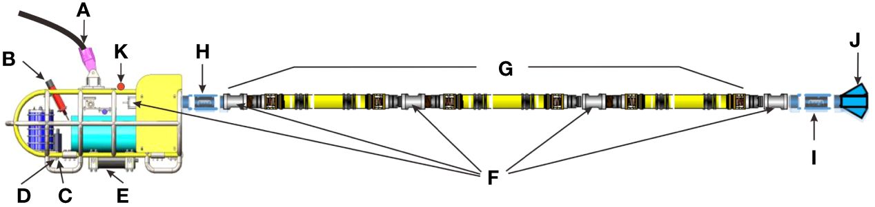
Figure 1 Components of the Kuiyang-ST2000 deep-towed high-resolution seismic system. (A: electro-optical cable; B: USBL; C: depth sensor; D: altimeter; E: plasma spark source; F: DTU; G: working section; H: front section; I: balance section; J: drogue; K: CTD).
2.2 Travel-time positioning
The travel-time positioning method is based on the geometric seismic principle, as shown in Figure 2.
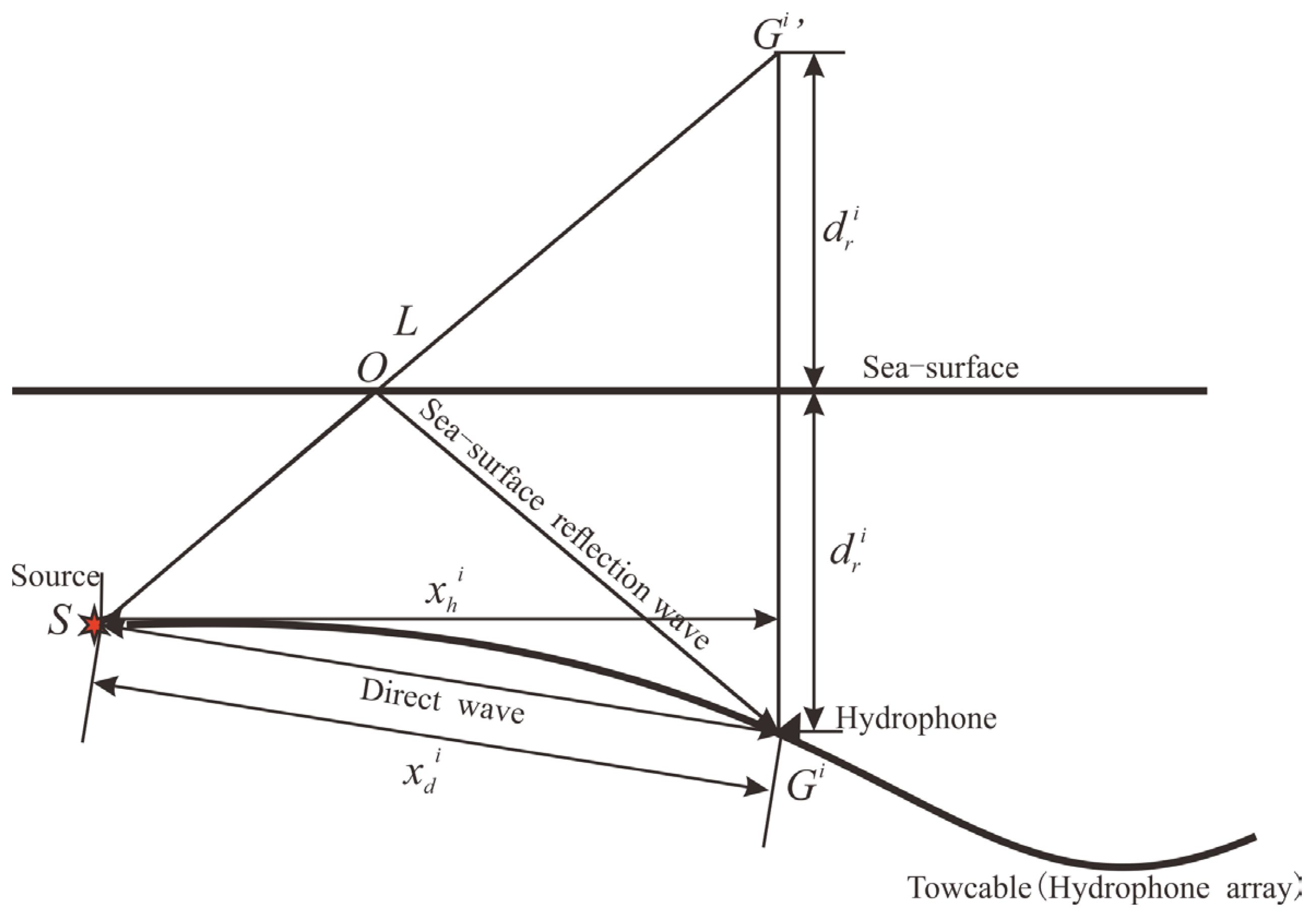
Figure 2 Travel-time positioning (direct and reflected wave paths) schematic diagram. (S, seismic source; Gi’, hydrophone mirror; Gi, hydrophone; dri, depth of hydrophone; ds, depth of seismic source; xhi, horizontal offset; xdi, travel distance of direct wave; L, travel distance of sea-surface reflection wave).
According to the geometric relationship (Eli, 2010), the position of hydrophones can be calculated by the following equations:
where and are the depth and horizontal offset of the ith hydrophone, respectively; and are the travel times of the direct wave and SSR wave picked by the ith hydrophone, respectively; vw is the average sound speed of seawater at full ocean depth; vf is the sound speed of seawater near the seafloor as measured by the CTD sensor; and ds is the seismic source depth measured by the depth sensor.
Figure 3 shows the one-shot seismic record (S2750) collected in the South China Sea in 2019. The seismic records include the travel times of the direct waves, reflected waves from the strata and reflected waves from the sea surface, as shown in Figures 3A–C, respectively. Finally, the array shape calculated by using the travel-time positioning method is shown in Figure 3D.
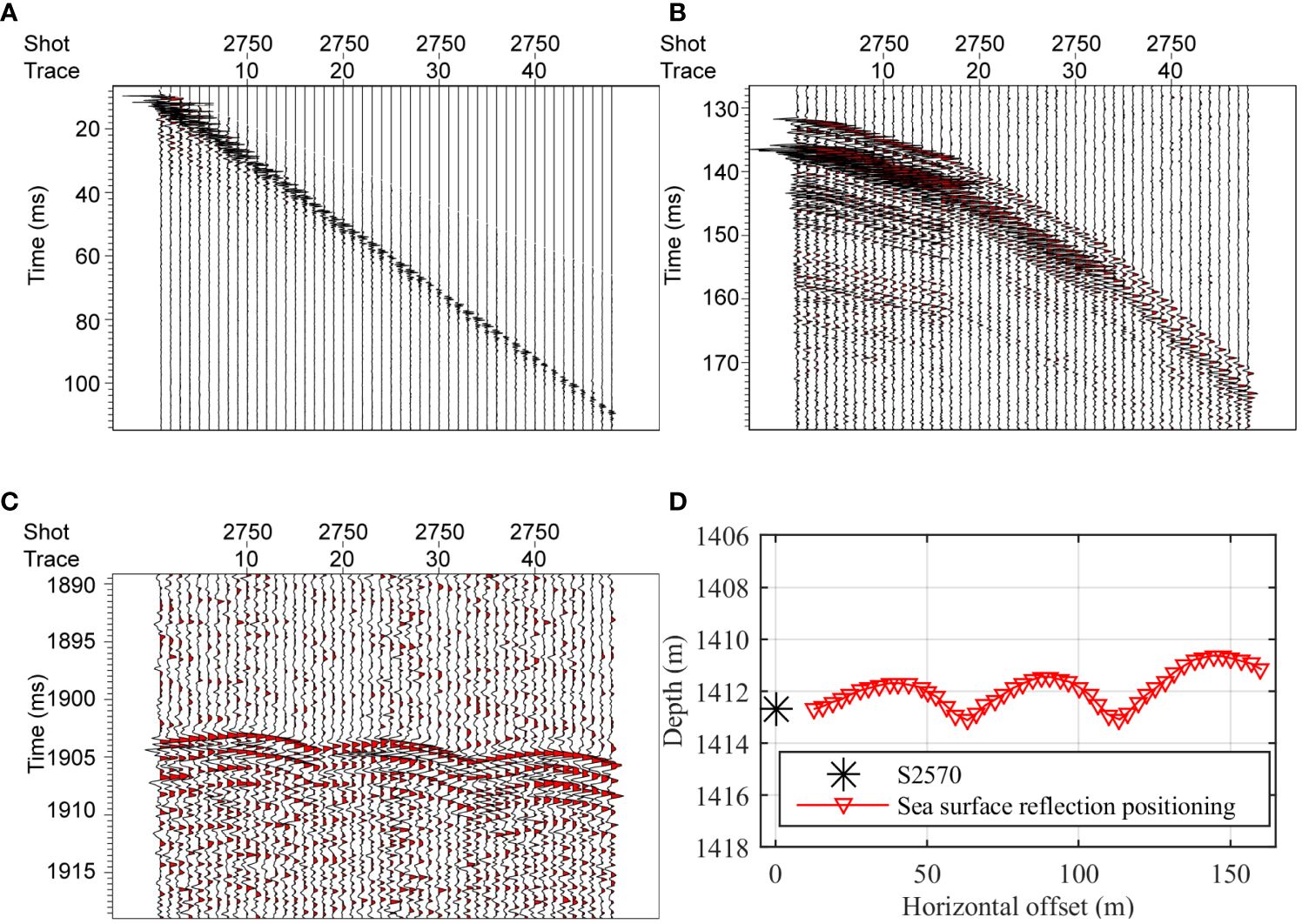
Figure 3 Examples of seismic records of sea surface reflection waves and travel-time positioning results. (A) Direct wave, (B) Seafloor reflection wave, (C) Sea surface reflection wave, (D) Array shape by travel-time positioning.
2.2.1 Positioning analysis
Because the sound speed of seawater varies with water depth, temperature and salinity, the assumption that the average sound speed of seawater is 1484.5 m/s is not accurate for every shot. Figure 4 shows the positioning results at velocities of 1483 m/s, 1485 m/s, and 1487 m/s. The positioning differences generated at velocities of 1483 m/s and 1487 m/s compared to 1485 m/s are illustrated in Figure 5. Even though the sound speed of seawater exhibits a small deviation, the array shape or inclination angle of the arrays with a still water level remains unchanged. The sound speed only affects the vertical position of the arrays. Fortunately, the vertical position of the seismic source is determined in a timely manner by the depth sensor, and the geometrical relationship between the towed vehicle and the arrays indicates that the vertical position of the seismic source can be used to adjust the sound speed of seawater. However, because the DTU between two adjacent working segments is made of stainless steel, the weight of the DTU is greater than its buoyancy. These redundant gravity forces the arrays to form a “W” shape, which makes it difficult to determine the geometrical relationship.
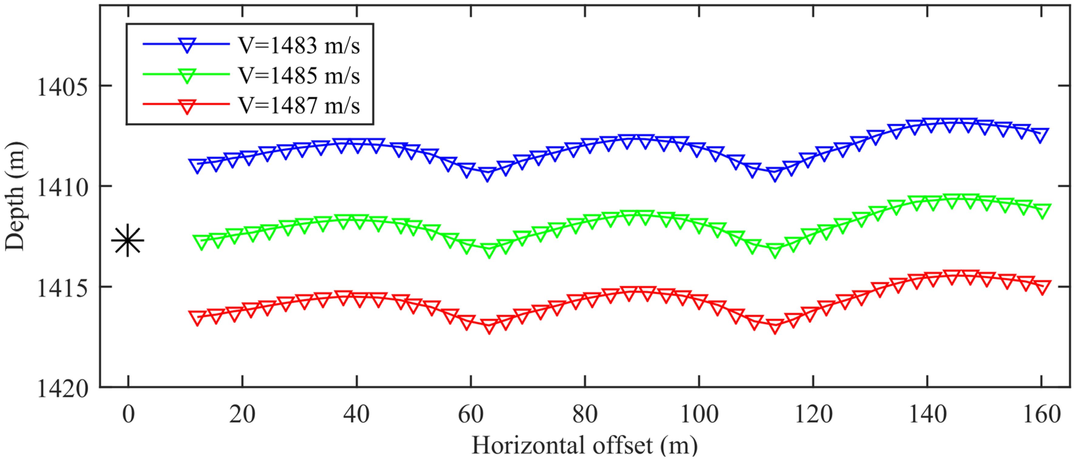
Figure 4 Travel-time positioning results with different acoustic velocities at shot point S2750.
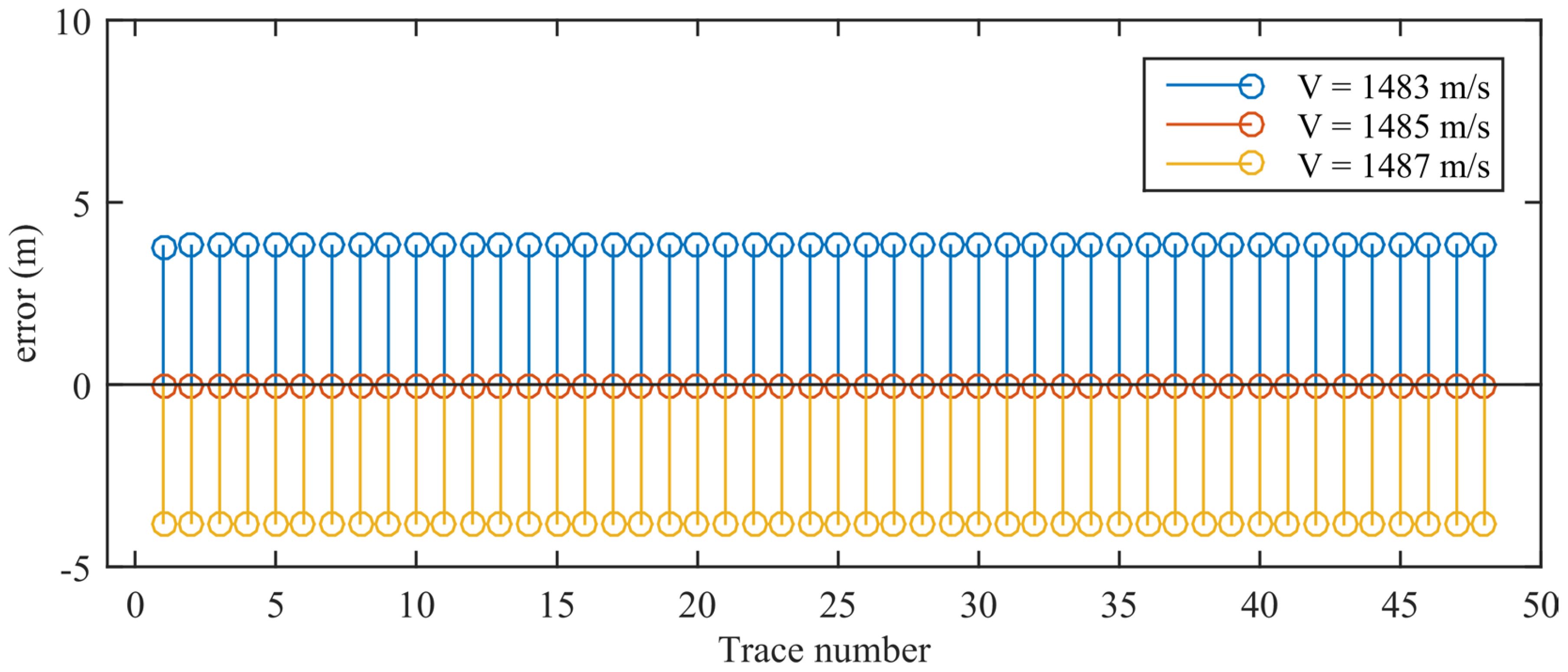
Figure 5 Depth differences with respect to the sound speed of seawater 1485 m/s.
2.3 Array shape correction
2.3.1 Floaters
The segment joint (DTU) is made of stainless steel and has a mass of 1.85 kg in air. The mass of occupied seawater is approximately 1.1 kg, so an excess of 0.75 kg should be balanced to reach zero buoyancy. Therefore, a floater is designed, as shown in Figure 6A. These devices can withstand pressures reaching a water depth of 3000 m. Thus, each floater provides equivalent buoyancy compared to the weight of the DTU. A photograph of the floater is shown in Figure 6B, and the arrays equipped with the floaters are shown in Figure 6C.
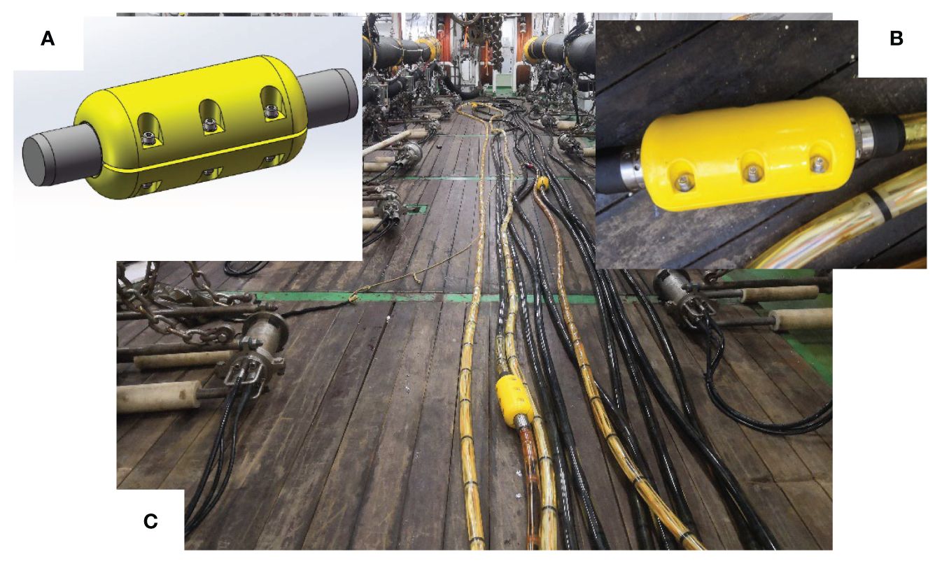
Figure 6 Floaters and arrays. (A) Buoyancy block model, (B) Installation of buoyancy blocks, (C) Array with buoyancy blocks installed.
2.3.2 Numerical model
To verify the performance of the floaters, an array model is established. The numerical modeling of the arrays and floaters are shown below. Via the lumped mass method, the array model is established with respect to the relative velocity element frame, as shown in Figure 7. The array is divided into 21 elements. The node connected to the towed vehicle is defined as the 1st node, while the end node is defined as the 22nd node.
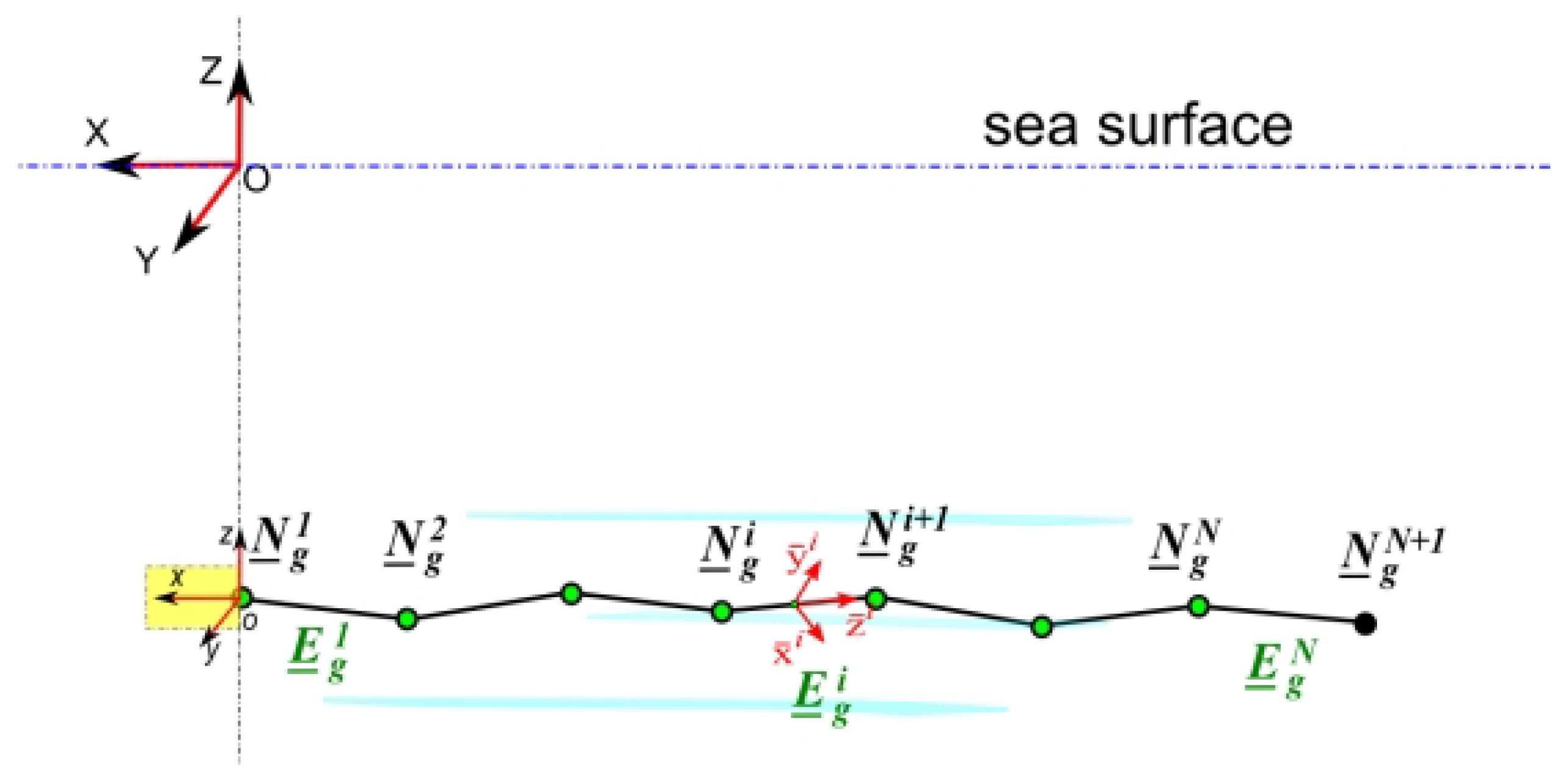
Figure 7 Modeling of arrays using the lumped mass method (Zhu et al., 2020).
The arrays are subjected mainly to internal tension and damping forces, hydrodynamic forces, and self-inertial forces in water. The tension and damping forces are calculated from the axial extension and the extension velocity, respectively, and are oriented in the same direction as the element orientation vector. According to the Morison formula, the drag resistance is proportional to the square of the relative velocity of the cable in water. These forces are simply expressed in Equation (3), as per.
where the cable tension is defined by the axial strain , elastic modulus E, and cable diameter . is defined by the current length of the ith element and the initial length , as shown in Equation (4). The damping force is expressed by the velocity difference between the terminal nodes in the element orientation direction. Cd is the damping coefficient of the cable, and is the node velocity with respect to the global frame. is the unit vector of the ith element orientation vector , which is obtained from the node position vectors and , as shown in Equation (4). The transformation matrix is used to convert the velocity from the global frame to the element-fixed frame. is the weight of the cable in water, and indicates that the force is oriented in the same direction as gravity. and are the densities of the cable and seawater, respectively. is the hydrodynamic force acting on the ith element, and Cn is the normal drag coefficient of the cable. and are the relative velocities of the ith element with respect to the element-fixed frame and global frame, respectively. The average velocity of the terminal nodes is used to express the velocity of the given element, as shown in Equation (4). is the velocity of the water particle at the ith node.
To consider the inertia force of the added mass, the mass matrix of the ith element in the element-fixed frame is given by Equation (5), where is the added mass coefficient. As the cable is continuous in the z-direction, the added mass is ignored along the cable axis.
The ith node mass matrix is expressed using the mass matrix of the elements and , as shown in Equation (6). The transformation matrix is used to convert the mass matrices from the element-fixed frame to the global frame.
Finally, the element loads are shared equally by two terminal nodes. Moreover, the governing equation for the ith node is determined by the loads acting on the (i-1)th and ith elements, as given in Equation (7). represents the acceleration of the ith node.
Because the weight is balanced with the buoyancy, the floater introduces only additional mass effects and hydrodynamic forces at the node position where the floater is mounted. Considering the mass of the DTU and floater, an additional mass of 2.87 kg is added to the mass matrix. The ocean current in the deep sea is very small, so the velocity and acceleration of the water particles are ignored here. Because the towing speed changes smoothly during formal towing, the additional mass effect of seawater is also ignored here. Finally, the additional drag force introduced by the floater is expressed by Equation (8), which is a function of the cross area and towing speed. and are the tangential and normal drag coefficients, respectively. and are the cross areas of the floater in the tangential and normal directions, respectively. The node velocity in the element frame is used to carry out the drag force, and , , and are the x-, y- and z-components of the node velocity at the ith floater, respectively. , , and are the x-, y-, and z-components of the additional drag generated by the floater in the element frame, respectively. Finally, these forces are converted to the global frame.
The modeling parameters of the arrays and floaters are listed in Tables 1 and 2, respectively. The drag coefficients of the floaters are measured via computational fluid dynamics simulation.

Table 1 Modeling parameters of the arrays.

Table 2 Cross-sectional area and drag coefficient of the floaters.
2.3.3 Correction effect
An array model with floaters was established, and the array shape under various towing conditions was studied via numerical simulation. The towing conditions include rising, diving and flat towing, as shown in Figure 8A. Because the floaters balance the weight of the DTUs, the arrays no longer form a “W” shape but become a simple convex curve, as illustrated in Figure 8. Because of the seismic source on the convex curve, a reasonable sound speed can be easily adjusted with the simple convex curve.
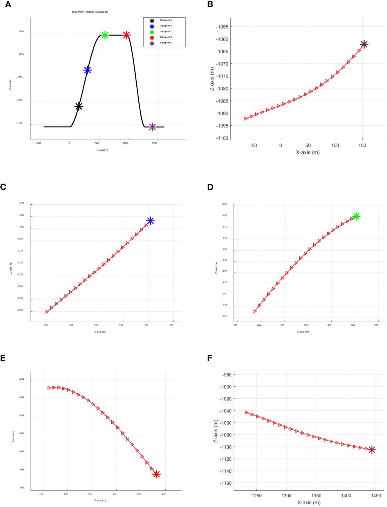
Figure 8 Array shape with floaters under different towing conditions. (A) Shot point distribution, (B) Array shape at shot (A), (C) Array shape at shot (B), (D) Array shape at shot (C), (E) Array shape at shot (D), (F) Array shape at shot (E).
The arrays equipped with floaters were used in the 2021 sea trial, and the location is indicated by the red point shown in Figure 9. The sea conditions were calm with ripples, and the water depth was approximately 1400-1600 m. The seismic records from the 2019 sea trial are shown in Figures 10A and C. Because floaters are not installed, the seismic records indicate that the sea surface reflection waves have broken lines and that the sea seafloor reflection waves exhibit a “W” shape. However, when the arrays are equipped with floaters, the seismic records exhibit simple convex curves, as shown in Figures 10B and D.

Figure 9 Location and water depth in the 2021 sea trial.
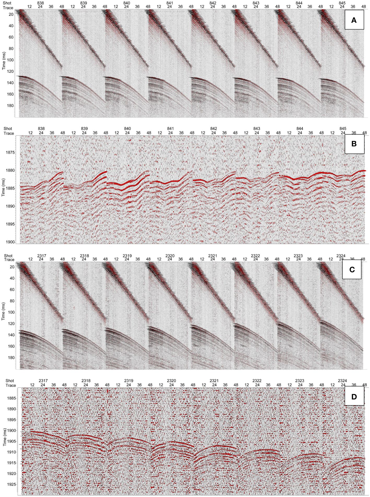
Figure 10 Recorded patterns in the 2019 (A: direct and seafloor reflection waves; B: sea surface reflection waves) and 2021 (C: direct and seafloor reflection waves; D: sea surface reflection waves) sea trials.
Two examples of sea surface reflection (SSR) records (Figures 11B, C) and travel-time positioning results (Figures 11D, F) are presented in Figure 11, revealing smooth curves in both the morphology of the sea surface reflection waves and the positioning structure of the towed array. Although few hydrophones jump out (S2129), the arrays equipped with floaters indeed exhibit a convex curve. Abnormal hydrophones are generated by phase distortion (waveform change), which is the general case in seismic exploration. Importantly, the seismic source is not on this convex curve (green dashed line), which indicates that the sound speed of seawater should be optimized and that abnormal hydrophones should be eliminated when forming the shape curve of seismic arrays.
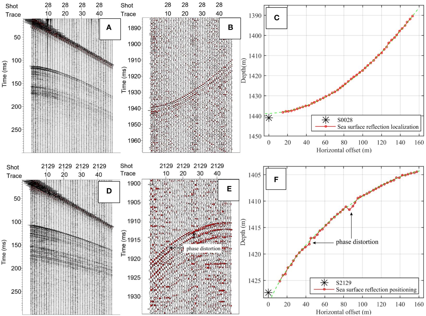
Figure 11 Wave field records and sea-surface reflection positioning results after array correction (A: direct and seafloor reflection wave at S0028; B: sea-surface reflection wave at S0028; C: sea-surface reflection positioning result at S0028; D: direct and seafloor reflection wave at S2129; E: sea surface reflection wave at S2129; and F: sea surface reflection positioning result at S2129).
3 Location modification
Both the numerical simulation and travel-time positioning results reveal that the array shape equipped with floaters is a simple convex curve under stable towing conditions. Because the depth of the seismic source is determined by the depth sensor and because the sound speed affects the vertical displacement of the arrays, if the assumed sound speed is greater than or less than the real velocity, then the seismic source is not on the convex curve. According to the weighted least squares polynomial fitting method, the sound speed of seawater can be optimized so that the seismic source and the arrays are on the same convex curve.
For a series of given points, which are the position coordinates of the source and hydrophones, the nth-order polynomial function f(x) used for fitting is shown by Equation (8b) (Parrilo and Sturmfels, 2003).
where a0, a1, … an are the polynomial coefficients. Except for the abnormal points, herein, all the hydrophones are used to fit this convex curve. The differences between the polynomial function f(x) and the yi values of the given points should be minimized, as shown in Equation (9) (Burden and Faires, 2010). wi represents the weight coefficient, xi represents the horizontal displacement of the hydrophone relative to the towed vehicle, and yi represents the vertical depth of the towed vehicle and hydrophones.
Because the weighted least squares method is used to determine the polynomial function f(x), this method is called weighted least squares polynomial fitting (Chen and Guo, 2023; Ke et al., 2023). The fitting quality can be evaluated by the goodness of fit R2 and the root mean square error S, as shown in Equations (10) and (11), respectively.
where is the average value of the hydrophone depth calculated by the travel-time positioning method f(xi) is the vertical depth of the hydrophone after fitting. The polynomial fitting becomes optimal when the goodness of fit R2 is close to 1 or the root mean square error S is the minimum.
To demonstrate the feasibility of the proposed method, two shot points, S2329 and S2350, were selected for positioning optimization. The sea floor is approximately flat at these two points. The seismic records of the SSR waves from the sea trial are shown in Figure 12. Based on the sound speed at the sea floor measured by the CTD sensor, the positioning results of the sea floor reflection (SFR) waves are shown in Figure 13. Additionally, the SSR positioning results of the SSR waves are also illustrated with the assumption that the average sound speed of seawater is 1484.5 m/s at the full depth of the survey area. The shape of the array cable generated by the SSR is similar to that generated by the SFR, but the seismic source is not on the extension line of the convex curve generated by the SSR. Because the sea floor is approximately flat at these two shots and because of the high speed of seawater at the sea floor measured by the CTD, the positioning results of the SFR are more accurate than those of the SSR. Therefore, the assumed average sound speed of seawater (vw) at the full depth of the survey area, i.e., 1484.5 m/s, needs to be adjusted.
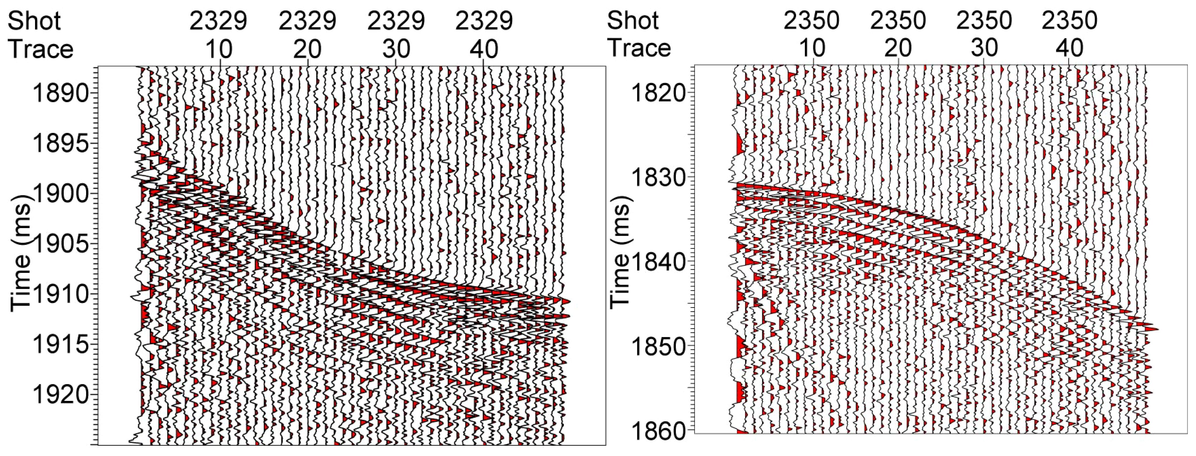
Figure 12 Seismic records from sea surface reflections at shots S2329 and S2350.
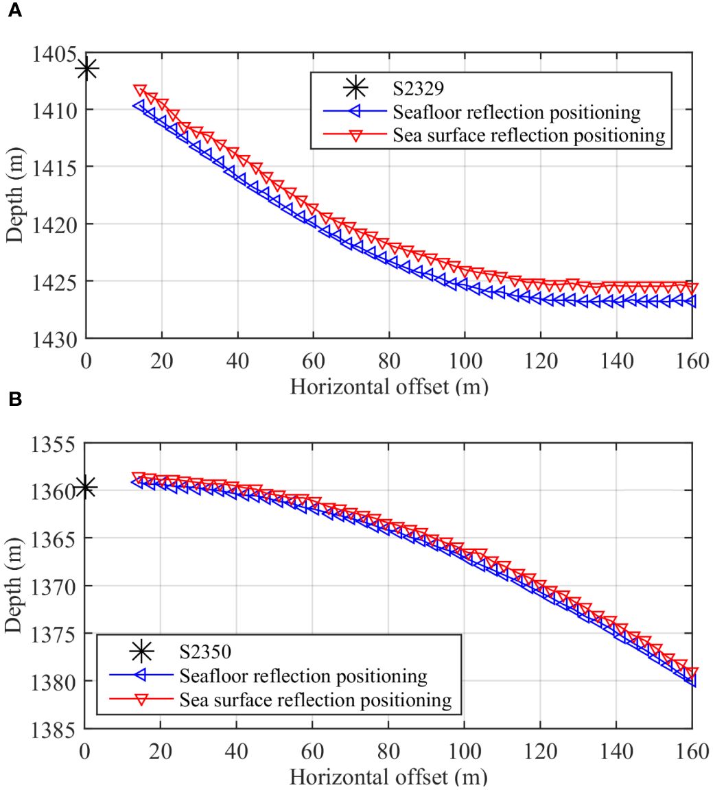
Figure 13 Positioning results calculated by the seafloor reflection wave and sea surface reflection wave. (A) Comparison of sea-surface reflection wave and seafloor reflection wave positioning results for shot point S2329, (B) Comparison of sea-surface reflection wave and seafloor reflection wave positioning results for shot point S2350.
The steps to optimize the travel-time positioning are as follows:
Step 1: The range of the sound speed of seawater at full depth (vmin, vmax) is defined according to experience (vmin= vw-5 m/s, and vmax= vw+5 m/s). The initial position of the arrays (xhi, dri) is determined by using Equations (1) and (2) with vw and vf.
Step 2: Source coordinates (0, ds) and hydrophone coordinates (xhi, dri) are combined in a data set {(0, ds), (xh1, dr1), (xh2, dr2), …, (xh48, dr48)}, and the weighted least squares polynomial is subsequently used for fitting. The weight coefficient w is set to 0.01 for the abnormal hydrophones, which are indicated by phase distortion in Figure 11. However, the weight coefficient for the other hydrophones is 1.0. One large root mean square error S is derived if the seismic source is not on the curve of the arrays calculated with the current vw, for example, ‘curve a’ or ‘curve c’, as shown in Figure 14. The optimized accuracy depends on the order of the polynomial fit, which is defined in this step. Taking S2329 and S2350 as examples, Table 3 shows the relationships among the polynomial fitting order, goodness of fit R2 and root mean square error S. As the fitting order increases, the goodness of fit approaches 1.0, and the root mean square error decreases. However, a long computation time is needed, and the stability of the fitting calculation decreases when the fitting order is larger than 4; thus, a fourth-order polynomial is sufficient herein. The polynomial function is f(x)=a0+a1x+a2x2+a3x3+a4x4.
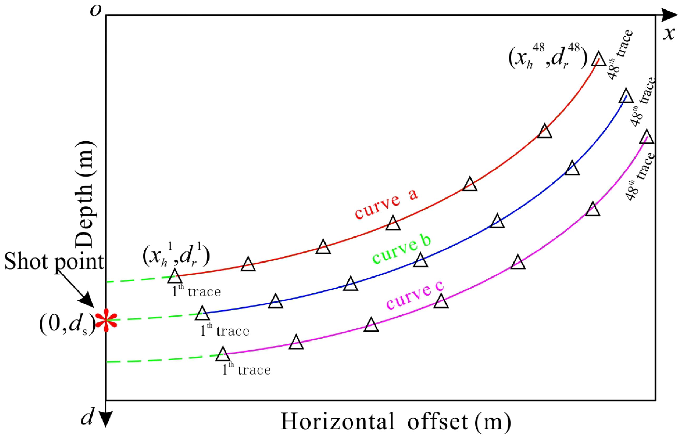
Figure 14 Polynomial fitting diagram.
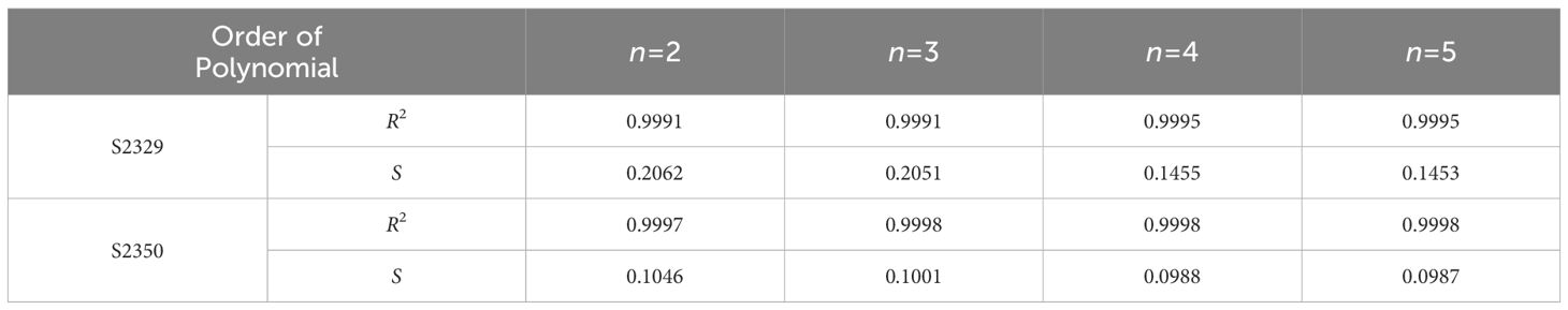
Table 3 Relationships between the fitting order and fitting quality for shots S2329 and S2350.
Step 3: The sound speed vi is increased by a step of 0.001 m/s from vmin to vmax, and the goodness of fit R2 and root mean square error S are calculated.
Step 4: The velocity vi with the maximum goodness of fit (R2) or the minimum root mean square error (S) is taken as the optimal sound speed for the final calculation of the array position (horizontal offset xroi and vertical depth droi). Moreover, the fitted value f(xi) is obtained. Because all the points {(0, ds), (xroi, f(xi))} are on a convex curve, such as curve b, whose extension (dotted green line) passes through the shot point, f(xi) is taken as the final hydrophone depth value, which also solves the phase distortion problem of abnormal hydrophones and reduces the influence of ocean waves.
According to the above processes, the array shape at shot S2329 was fitted by using a fourth-order polynomial, i.e., f(x)=a0+a1x+a2x2+a3x3+a4x4. The coefficients and fitting parameters of the polynomial are shown in Table 4. The goodness of fit is 0.9995, and the root mean square error is only 0.1355. Theoretically, the seismic source depth ds is the intercept of the fitting polynomial on the depth axis; thus, it is equal to the constant term a0. The fitting result a0 shown in Table 4 is approximately equal to the seismic source depth ds, indicating that the fitting quality is high.

Table 4 Polynomial fitting parameters at shot 2329.
The comparison between the optimization results and the initial positioning results is shown in Figure 15, and the root mean square error and goodness of fit are shown in Figure 16. Compared to that of seafloor reflection positioning, the depth errors in SSR positioning before and after polynomial fitting are shown in Figures 17A and B, respectively. These results indicate that the polynomial fitting method is accurate and that the absolute values of the errors are less than 0.15 m (~0.1 ms).
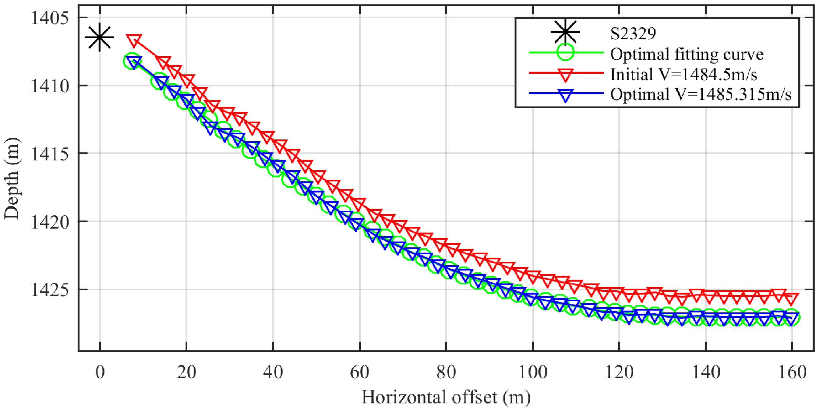
Figure 15 Travel-time positioning before and after correction at shot S2329.
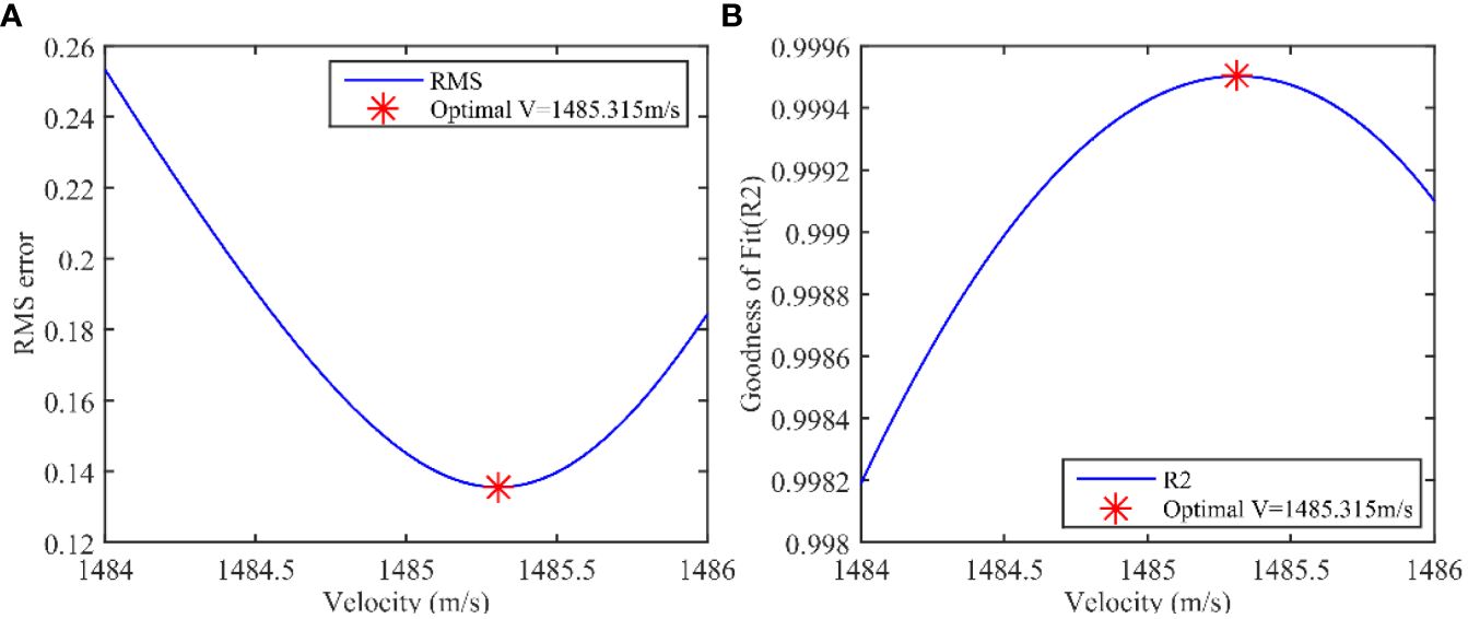
Figure 16 Fitting quality at shot S2329. (A) Root mean square error, (B) Goodness of fit.
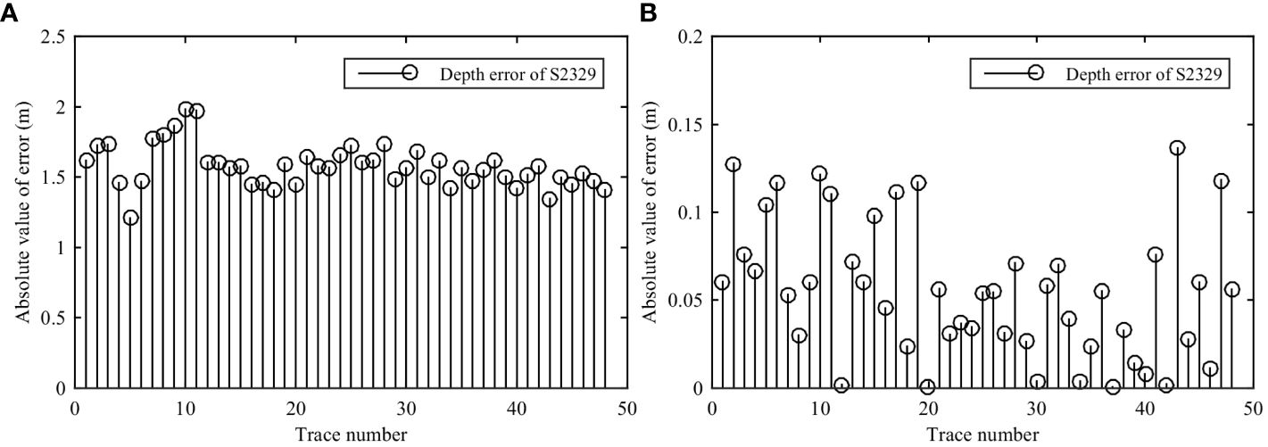
Figure 17 Depth error of sea surface reflection positioning compared to seafloor reflection positioning at shot S2329. (A) Before optimization, (B) After optimization.
Similarly, the array shape at shot point S2350 was fitted by the proposed method. The parameters of the fitted polynomials are shown in Table 5. The goodness of fit is 0.9940, and the root mean square error is only 0.0660. In addition, the fitted polynomial a0 is equal to the seismic source depth ds, indicating that the fitting is optimal.

Table 5 Polynomial fitting parameters at shot point S2350.
The array shapes obtained by the polynomial fitting method and by the assumed average speed of 1484.5 m/s are shown in Figure 18. The root mean square error and goodness of fit are shown in Figure 19. Compared to those of the seafloor reflection positioning, the depth errors in SSR positioning before and after polynomial fitting are shown in Figures 20A and B, respectively. The absolute values of the depth errors are less than 0.14 m (~0.09 ms) after polynomial fitting.
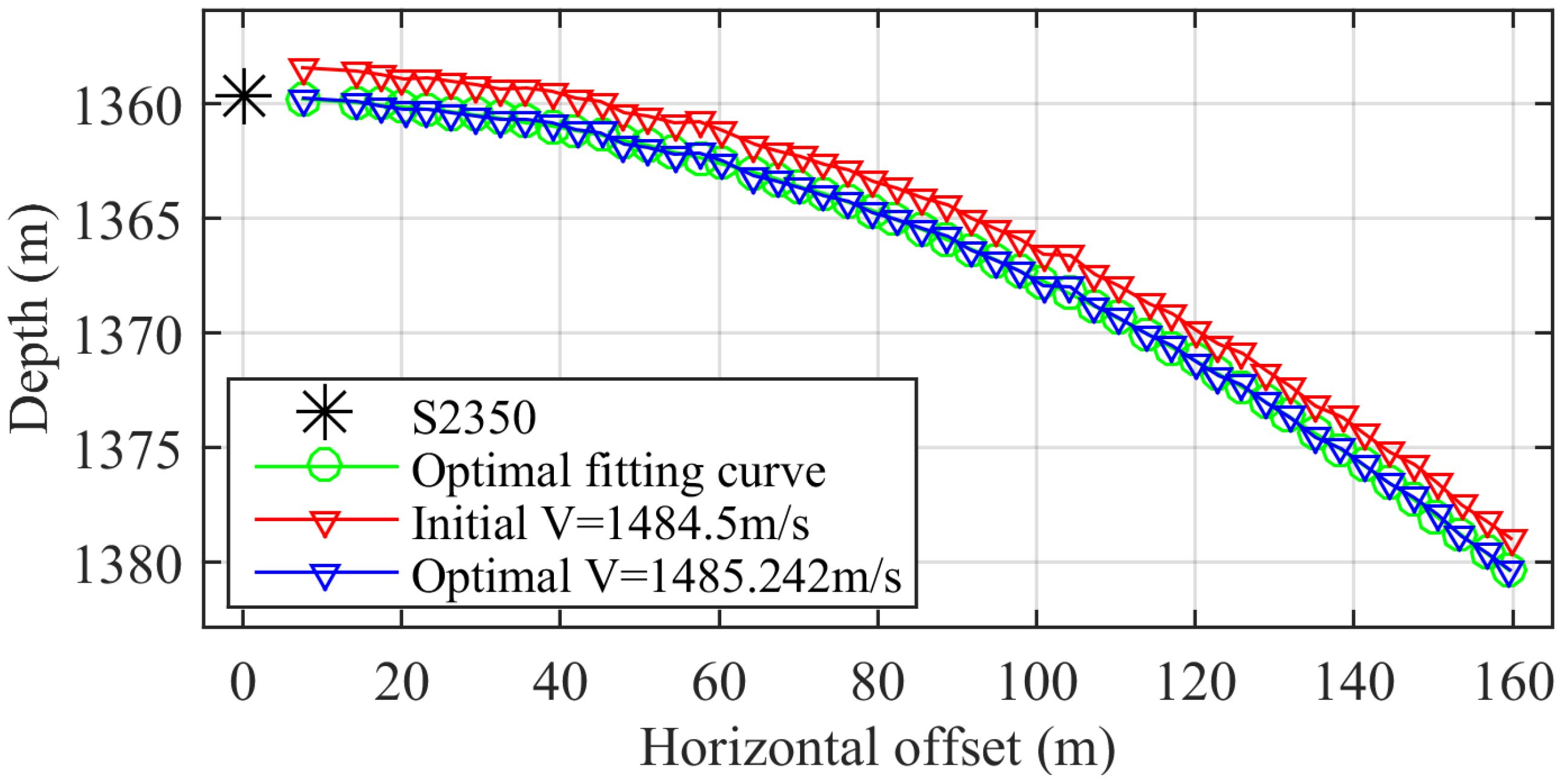
Figure 18 Travel-time positioning before and after correction at shot S2350.
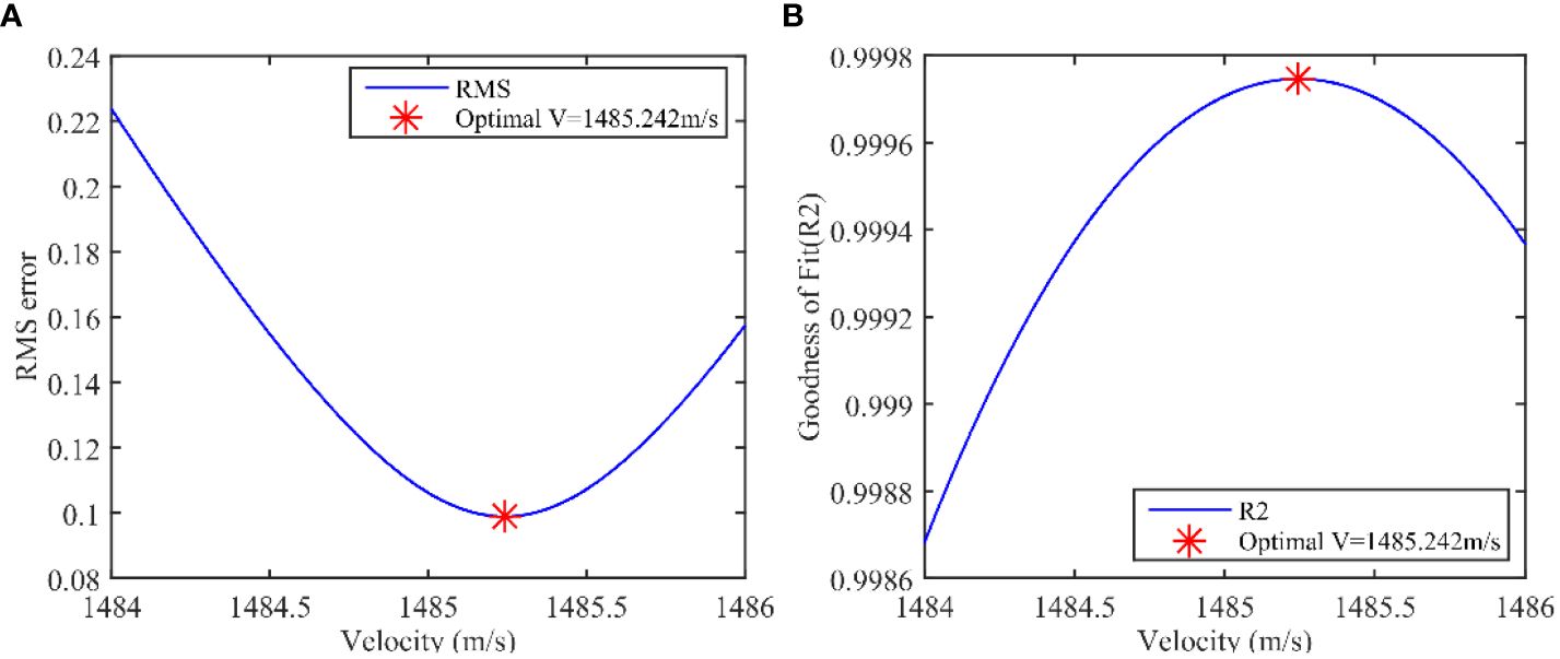
Figure 19 Fitting quality at shot point S2350. (A) Root mean square error, (B) Goodness of fit.
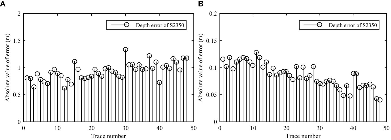
Figure 20 Depth error of sea surface reflection positioning compared to seafloor reflection positioning at shot point S2350. (A) Before optimization, (B) After optimization.
Additionally, the positions of the arrays at shot points S0028 and S2129 were also corrected according to the above processes. The polynomial fitting parameters, goodness of fit R2 and root mean square error S for the array positioning are listed in Table 6. The seismic source is not on the convex curve, generating an assumed velocity of 1484.5 m/s, as shown in Figure 21. However, the sound speed of seawater is optimized by the polynomial fitting method, and the seismic source and the positioning results of the arrays are on the same convex curve (dashed green line). In addition, although there are phase distortions in some channels at shot S2129, the weighted least squares polynomial method overcomes inaccurate positioning.
Table 6 Polynomial fitting parameters at shot points S0025 and S2129.
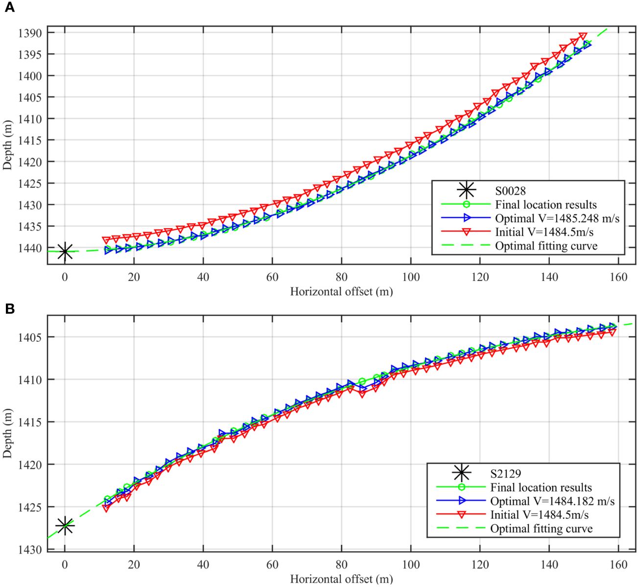
Figure 21 Travel-time positioning before and after correction. (A) Comparison of the corrected sea-surface reflection wave positioning results and seafloor reflection wave positioning results for shot point S0028, (B) Comparison of the corrected sea-surface reflection wave positioning results and seafloor reflection wave positioning results for shot point S2129.
4 Application
The prestack shot gathers in the sea trial with Kuiyang-ST2000 conducted in 2021 in the Qiongdongnan area in the South China Sea are selected, as shown in Figure 8. The main acquisition parameters of the deep-towed multichannel seismic datasets are as follows: the source energy is 3000 J, shot spacing is 6.25 m, trace spacing is 3.125 m, minimum offset is 12.5 m, trace number is 48, recording duration is 3000 ms, and sampling rate is 8 kHz.
We utilize the SSR travel-time positioning method described in Section 2.2 to obtain the initial values of the towed array. Based on the characteristics of the towed array structure described in Section 2.3, we applied the correction method outlined in Chapter 3 to determine the accurate positions of the hydrophone array in the towed cable. Figure 22A shows the velocity spectra of common middle point (CMP) gathered on survey lines corrected by floating datum (with reference to the datum setting as land complex surface data processing; the shot point and hydrophone point are placed on a relatively smooth float datum) in seismic data processing (Yilmaz, 2001). The focusing of the energy group of the velocity spectrum calculated by the semblance coefficient method (Kirlin, 1992) is not highly concentrated in either the deep layer or the shallow layer before positioning correction. The focusing of the energy group in the velocity spectrum is highly concentrated in both the deep layer and shallow layer after correction, as shown in Figure 22B, and the resolution of the velocity spectrum is notably improved. The preliminary stack profiles before and after correction are shown in Figure 23. The phase continuity and signal-to-noise ratio are obviously improved after correction, as shown in Figure 23B, compared with the uncorrected (Figure 23A), especially within the yellow boxes, and this approach can accurately describe the geological structure morphology under the seabed.
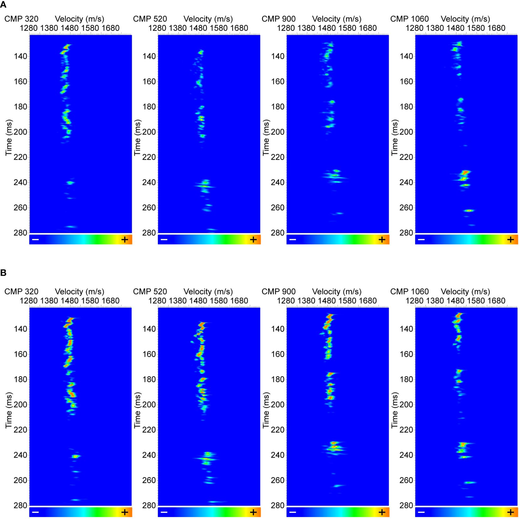
Figure 22 Velocity semblance panels before and after travel-time positioning correction. (A) Before travel-time positioning correction. (B) After travel-time positioning correction.
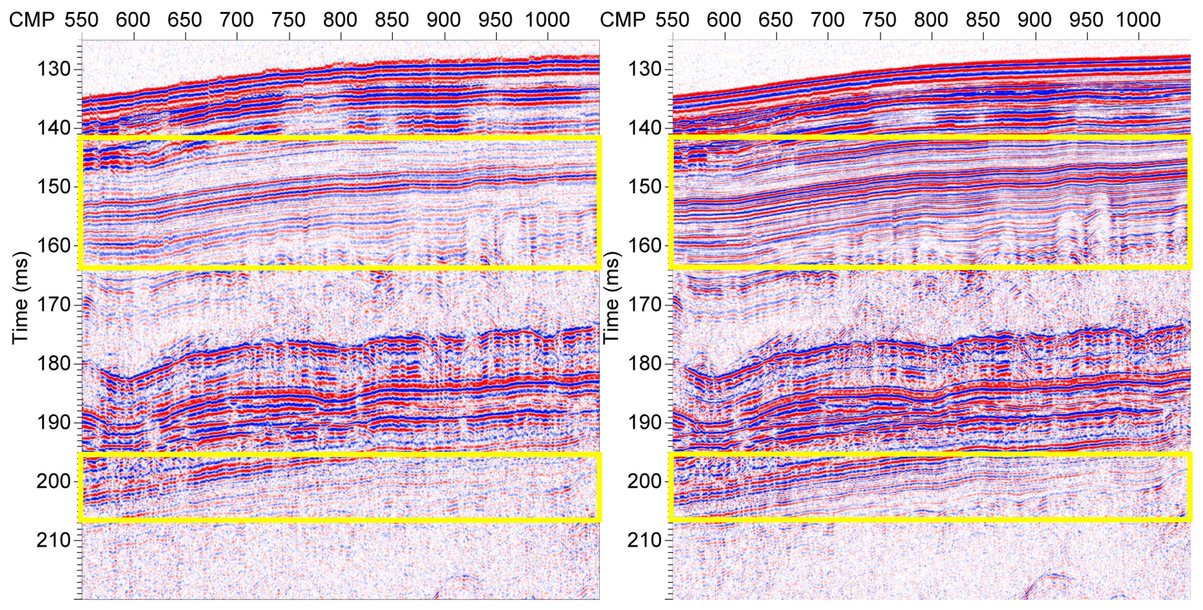
Figure 23 Seabed stack profile before (left) and after (right) travel-time positioning correction.
5 Conclusions
To correct for the “W” shape of seismic arrays, floaters were installed at the DTUs of the Kuiyang-ST2000 deep-towed seismic system. The corrected arrays presented a simple smooth convex curve during towing conditions, which was demonstrated by both the numerical simulation and travel-time positioning of the sea trial. Given the geometrical relationship between towed vehicles and seismic arrays, the weighted least squares polynomial fitting method is proposed herein to optimize the average sound speed of seawater at full ocean depth. The final positioning accuracy (0.15 m/~0.1 ms) was less than the system sampling interval of 0.125 ms, which met the accuracy requirements of the Kuiyang-ST2000 deep-towed seismic system. Additionally, the energy groups of the velocity spectrum were also highly concentrated in both the deep layer and shallow layer after positioning correction, and the signal-to-noise ratio and resolution of superposition imaging were effectively improved in the seabed stack profile. The conclusions of general validity are listed here for reference.
(1) The array shape follows a simple smooth convex curve when the additional weights of the DTUs are balanced by floaters.
(2) Weighted least squares polynomial fitting is an efficient method for obtaining the accurate average sound speed of seawater at full ocean depth under the constraint that the seismic source is located on a smooth convex curve.
(3) Because seafloor reflection positioning is limited by the constraint that the seafloor is flat, sea surface reflection positioning can be widely used when the average sound speed at full ocean depth is known.
(4) The phase distortions generated by abnormal hydrophones can be repaired via the proposed polynomial fitting method.
Data availability statement
The original contributions presented in the study are included in the article/supplementary material. Further inquiries can be directed to the corresponding author.
Author contributions
ZW: Data curation, Writing – original draft, Writing – review & editing, Formal analysis, Investigation, Methodology, Resources, Visualization. YP: Data curation, Funding acquisition, Project administration, Resources, Writing – original draft, Writing – review & editing. XQZ: Formal analysis, Methodology, Writing – review & editing. KL: Data curation, Resources, Writing – review & editing. XBZ: Formal analysis, Investigation, Visualization, Writing – review & editing. LZ: Writing – review & editing. XL: Investigation, Software, Visualization, Writing – review & editing.
Funding
The author(s) declare financial support was received for the research, authorship, and/or publication of this article. This work was supported by the National Key Research and Development Program of China (No. 2023YFC2811200, No. 2016YFC0303901);National Natural Science Foundation of China (Grant Nos. 51909145 and 42106072); Laoshan Laboratory (No. LSKJ202203604).
Acknowledgments
The authors would like to acknowledge FunctionBay Inc. and Prometech Software Inc. for providing license files of RecurDyn and Particleworks, respectively.
Conflict of interest
The authors declare that the research was conducted in the absence of any commercial or financial relationships that could be construed as a potential conflict of interest.
Publisher’s note
All claims expressed in this article are solely those of the authors and do not necessarily represent those of their affiliated organizations, or those of the publisher, the editors and the reviewers. Any product that may be evaluated in this article, or claim that may be made by its manufacturer, is not guaranteed or endorsed by the publisher.
References
Burden R. L., Faires J. D. (2010). Numerical Analysis. 9th ed (Brooks Cole). Boston: Cengage Learning Press.
Chapman N. R., Gettrust J. F., Walia R., Hannay D., Spence G. D., Wood W. T., et al. (2002). High-resolution, deep-towed, multichannel seismic survey of deep-sea gas hydrates off western Canada. Geophysis 67, 1038–1047. doi: 10.1190/1.1500364
Che Z., Wang J., Zhu J., Zhang B., Zhang Y., Wu Y. (2021). Real-time array shape estimation method of horizontal suspended linear array based on non-acoustic auxiliary sensors. IEEE Access. 9, 90500–90509. doi: 10.1109/ACCESS.2021.3061446
Chen H., Guo L. (2023). Convergence of adaptive MPC for linear stochastic systems. Sci. CHINA-INFORMATION Sci. 66, (5). doi: 10.1109/ACCESS.2021.3061446
Colin F., Ker S., Marsset B. (2020). Fine-scale velocity distribution revealed by datuming of very-high-resolution deep-towed seismic data: Example of a shallow-gas system from the western Black Sea. Geophysics 85, B181–B192. doi: 10.1190/geo2019-0686.1
Eli M. (2010). The Pythagorean Theorem: A 4,000-Year History (New Jersey: Princeton University Press).
Fagot M. G., Gholson N. H., Moss G. J., Milburn D. A. (1980). Deep-towed geophysical array system development program review. Navel Ocean Res. Dev. Activity NSTL Station MS.
Fikes A. C., Safaripour A., Bohn F., Abiri B., Hajimiri A. (2019). Flexible, conformal phased arrays with dynamic array shape self-calibration. 2019 IEEE MTT-S International Microwave Symposium (IMS). IEEE, 1458–1461. doi: 10.1109/MWSYM.2019.8701107
He T., Spence G. D., Wood W. T., Riedel M., Hyndman R. D. (2009). Imaging a hydrate-related cold vent offshore Vancouver Island from deep-towed multichannel seismic data. Geophysics 74, B23–B36. doi: 10.1190/1.3072620
Howard B. E., Syck J. M. (1992). Calculation of the shape of a towed underwater acoustic array. IEEE J. ocea. eng. 17, 193–203. doi: 10.1109/48.126976
Ke K., Zhang C. M., Wang Y. Q., Zhang Y. J., Yao B. L. (2023). Single underwater image restoration based on color correction and optimized transmission map estimation. Masure. Sci. Techol. 34, (5). doi: 10.1088/1361-6501/acb72d
Ker S., Marsset B., Garziglia S., Le Gonidec Y., Gibert D., Voisset M., et al. (2010). High-resolution seismic imaging in deep sea from a joint deep-towed/OBH reflection experiment: application to a Mass Transport Complex offshore Nigeria. GEOPHYS. J. Int. 182, 1524–1542. doi: 10.1111/j.1365-246X.2010.04700.x
Kirlin R. L. (1992). The relationship between semblance and eigenstructure velocity estimators. Geophysics. 57 (8), 1027–1033. doi: 10.1190/1.1443314
Kong F., He T., Spence G. D. (2012). Application of deep-towed multichannel seismic system for gas hydrate on mid-slope of northern Cascadia margin. Sci. China-Earth Sci. 55, 758–769. doi: 10.1007/s11430-012-4377-4
Krödel S., Thomé N., Daraio C. (2015). Wide band-gap seismic metastructures. Extreme Mech. Lett. 4, 111–117. doi: 10.1016/j.eml.2015.05.004
Lan H., Ding Y. (2012). Ordering, positioning and uniformity of quantum dot arrays. Nano Today 7, 94–123. doi: 10.1016/j.nantod.2012.02.006
Lu F., Milios E., Stergiopoulos S., Dhanantwari A. (2003). New towed-array shape-estimation scheme for real-time sonar systems. IEEE J. ocea. eng. 28, 552–563. doi: 10.1109/JOE.2003.816694
Marsset B., Ker S., Thomas Y., Colin F. (2018). Deep-towed high resolution seismic imaging II: Determination of P-wave velocity distribution. Deep-Sea Res. Part I-Oceanogr. Res. Pap. 132, 29–36. doi: 10.1016/j.dsr.2017.12.005
Marsset B., Menut E., Ker S., Thomas Y., Regnault J. P., Leon P., et al. (2014). Deep-towed High Resolution multichannel seismic imaging. Deep-Sea Res. Part I-Oceanogr. Res. Pap. 93, 83–90. doi: 10.1016/j.dsr.2014.07.013
Nanni U., Roux P., Gimbert F., Lecointre A. (2022). Dynamic imaging of glacier structures at high-resolution using source localization with a dense seismic array. Geophys. Res. Lett. 49, e2021GL095996. doi: 10.1029/2021GL095996
Parrilo P. A., Sturmfels B. (2003). Minimizing polynomial functions. Algorithmic and quantitative real algebraic geometry, DIMACS Series in Discrete Mathematics and Theoretical Computer Science 60, 83–99.
Pei Y., Wen M., Zhang L., Yu K., Kan G., Zong L., et al. (2022). Development of a high-resolution deep-towed multi-channel seismic exploration system: Kuiyang ST2000. J. Appl. Geophys. 198, 104575. doi: 10.1016/j.jappgeo.2022.104575
Rowe M. M., Gettrust J. F. (1993). Faulted structure of the bottom simulating reflector on the Blake Ridge, Western North-Atlantic. Geology 21, 833–836. doi: 10.1130/0091-7613(1993)021<0833:FSOTBS>2.3.CO;2
Varypaev A., Kushnir A. (2020). Statistical synthesis of phase alignment algorithms for localization of wave field sources. Multidimens. Syst. Signal Process. 31, 1553–1578. doi: 10.1007/s11045-020-00722-3
Vickery K. (1998). “Acoustic positioning systems. A practical overview of current systems,” in Proceedings of the 1998 Workshop on Autonomous Underwater Vehicles (Cat. No. 98CH36290) (IEEE), 5–17. doi: 10.1109/AUV.1998.744434
Walia R., Hannay D. (1999). Source and receiver geometry corrections for deep towed multichannel seismic data. Geophys. Res. Lett. 26, 1993–1996. doi: 10.1029/1999GL900402
Wei Z., Pei Y., Liu B. (2020). A new deep-towed,multi-channel high-resolution seismic system and its preliminary application in the South China Sea. Oil Geophys. Prospect. 55, 965–972. doi: 10.13810/j.cnki.issn.1000-7210.2020.05.004
Yilmaz Ö. (2001). Seismic data analysis: Processing, inversion, and interpretation of seismic data. Soc. Explor. geophys. doi: 10.1190/1.9781560801580
Keywords: deep-towed multichannel seismic system, array shape, array positioning, sound speed at full ocean depth, polynomial fitting
Citation: Wei Z, Pei Y, Zhu X, Liu K, Zhang X, Zong L and Li X (2024) A high-precision positioning method for deep-towed multichannel seismic arrays. Front. Mar. Sci. 11:1351327. doi: 10.3389/fmars.2024.1351327
Received: 06 December 2023; Accepted: 05 July 2024;
Published: 29 July 2024.
Edited by:
Kai Zhao, Nanjing Tech University, ChinaReviewed by:
Chuanlin He, Harbin Institute of Technology, ChinaHiroyuki Matsumoto, Japan Agency for Marine-Earth Science and Technology (JAMSTEC), Japan
Shaowei Zhang, Chinese Academy of Sciences (CAS), China
Copyright © 2024 Wei, Pei, Zhu, Liu, Zhang, Zong and Li. This is an open-access article distributed under the terms of the Creative Commons Attribution License (CC BY). The use, distribution or reproduction in other forums is permitted, provided the original author(s) and the copyright owner(s) are credited and that the original publication in this journal is cited, in accordance with accepted academic practice. No use, distribution or reproduction is permitted which does not comply with these terms.
*Correspondence: Yanliang Pei, cGVpeWFubGlhbmdAZmlvLm9yZy5jbg==