 Jiahui Wang
 Zhiqiang Cui2†
 Xu Liu
- 1School of Information Engineering, Zhejiang Ocean University, Zhoushan, China
- 2Hydroacoustics Technology Co., Ltd., Zhoushan, China
- 3Fujian Provincial Key Laboratory of Marine Physical and Geological Processes, Xiamen, China
- 4Unit 92578 of the People’s Liberation Army, Beijing, China
- 5National Engineering Research Center of Marine Facilities Aquaculture, Zhejiang Ocean University, Zhoushan, China
- 6School of Marine Science and Technology, Zhejiang Ocean University, Zhoushan, China
Introduction: Existing methods primarily focus on earth acoustic parameters inversion under specific layered structures. However, they face challenges with experimental data from unknown seabed stratification, hindering accurate parameter inversion.
Methods: To address this, a novel algorithm combines Back Propagation Neural Network (BPNN) for distinguishing seabed stratification and inverting acoustic parameters. Simulated sound pressure data disturb seabed parameters as input, enabling feature recognition for training the neural network inversion model. Acoustic parameters are then estimated under identified stratification using the sound field model.
Results: The inversion model is validated using simulation and pool shrinkage data. Results show the neural network model effectively stratifies simulation and experimental data, providing accurate inversion results for acoustic parameters corresponding to distinct layers.
Discussion: The neural network model's accuracy and practicality are confirmed through hierarchical judgment of scale test data and acoustic parameter inversion. This approach introduces a new perspective for shallow sea acoustic parameter inversion, offering a promising application scenario.
1 Introduction
Underwater acoustic parameters are important physical parameters for studying acoustic propagation characteristics in shallow seas. With the development of acoustic technology and the popularity of machine algorithms, it is convenient and efficient to in-vert underwater acoustic parameters using acoustic methods (Li and Zhang, 2017). Aiming at parameters inversion, a large number of underwater acoustic parameters inversion works have been carried out by predecessors, and many methods for underwater acoustic parameters in-version have been developed, such as the acoustic parameters inversion method based on transmission loss (Dragna and Blanc-Benon, 2017), the seafloor sediment parameters were estimated using the genetic algorithm and bottom reflection loss curve with wide grazing angles (Wang et al., 2023), a solution to the problem of stratified seabed parameters estimation using the sound field matching meth-od with vertical angle spectra (Xue et al., 2023),three-dimensional sediment modelling and inversion of geoacoustic parameters using a cross-dimensional Bayesian approach with wideband acoustic sources (Ke et al., 2013), the acoustic signal arrival time (Wang et al., 2023), and the waveguide dispersion characteristics (Kerzhakov and Kulinich, 2016). Among them, the most widely used methods can be summarized as the matching field inversion of underwater acoustic parameters by using the physical characteristics of underwater acoustic signals combined with the global optimization algorithm (Potty et al., 2017). Different physical characteristics are used as the forward model, and then through various optimization algorithms, such as Genetic algorithms (GA) and Simulated Annealing algorithms (SA), the objective function is solved to obtain the parameters results to be in-verted. Existing studies focus on the inversion calculation of geoacoustic parameters un-der specific stratification structures (Wang, 2008; Zhu et al., 2013). The statistical characteristics of the hydroacoustic echo signal reflected from the seabed, which produces a sudden change, reflect the existence of the seabed boundary. That is, on behalf of the seabed, there is a layered structure. There is no coverage of the sedimentary layer in the base. The seabed can be regarded as a semi-infinite seabed (Gerstoft, 1994). Such as the base is covered by a layer of sedimentary layer. As a result of this time, the physical characteristics of the physical characteristics of the seabed and semi-infinite seabed have a large difference and cannot be used to solve a similar problem of the semi-infinite seabed (Zhao et al., 2023). And so the previous introduction of the stratified seabed model, due to the oceanic motion and crustal movement of a stochastic, and so the base covered by the number of sedimentary layers is also not given to a fixed number of layers, it needs to be reflected according to the characteristics of the signal (Zhu et al., 2023b). When processing experimental data under unknown seabed stratification, the inversion results of geoacoustic parameters following the stratification cannot be accurately given. In addition, when the existing classical optimization algorithms are applied, the iterative optimization calculation between the input data and the optimal solution not only consumes a lot of computing time, but also easily falls into the optimal local solution (Zhu et al., 2023a).
Given the performance advantages of neural network algorithms in data processing, many scholars have tried to apply neural network models in classification research and parameters inversion in recent years. Chen, Yang et al. used migration learning and convolutional neural network to study the classification of sediments such as sand, reef and mud (Song and Wang, 2022). Huang has applied the Convolutional neural network (CNN) model to the geo-physical inversion, successfully realizing the inversion of some geological parameters, and proving that the neural network model has strong generalization applicability in the inversion problem (Feng et al., 2022). Wu et al. used a single-hidden layer feedforward neural network an extreme learning machine to perform inversion in shallow water depth remote sensing and obtained relatively accurate inversion results (Chen et al., 2022). Li, Wen et al. applied the back-propagation neural network (BPNN) model to electromagnetic inversion and effective wave height field parameters inversion. They improved the differential evolution algorithm of the BPNN model to achieve a more efficient and accurate inversion target (Yang et al., 2021). Due to BPNN’s powerful nonlinear fitting capability, this algorithm can automatically learn and identify hidden patterns and relationships from data. When dealing with the acoustic and geological complexities of shallow waters, it can provide highly accurate and reliable results. Therefore, using BPNN for seabed stratification and acoustic parameters inversion in shallow seas is worth further study (Pang et al., 2021).
Inspired by the numerous successful applications of neural network models in target classification and parameters inversion, this study employs the BPNN for hierarchical structure assessment and geoacoustic parameters inversion. Focused on the shallow-sea sound pressure field, the research employs neural network algorithms to establish a relational model between the predicted sound pressure field and the acoustic parameters to be retrieved (Wang et al., 2022). Subsequently, the model is utilized to achieve accurate hierarchical structure assessment and geoacoustic parameters inversion within a predefined shallow-sea environment. The study is divided into four main sections: the first section provides an overview of geoacoustic parameters inversion methods based on sound pressure fields. The subsequent section introduces the methods of hierarchical assessment and geoacoustic parameters inversion using the BPNN models. The third section assesses the application’s effectiveness and the performance of the neural network models through simulation and experimental data. Finally, the research concludes its findings.
2 Method
2.1 Forward modeling of shallow sea sound field
Acoustic parameters in shallow seas are important environmental parameters that determine the distribution characteristics of acoustic fields in shallow sea environments. The change of acoustic parameters in the seabed will have a significant impact on the distribution characteristics of the acoustic pressure field in water so that the geoacoustic parameters can be retrieved from the measurement data of the acoustic pressure field in the shallow sea (Kerzhakov and Kulinich, 2016).
In the model, the harmonic point source is located on the symmetry axis of the cylindrical coordinate. In shallow sea waveguide environments, the characteristics of seafloor sediments play an indispensable role in influencing marine acoustic fields. Various parameters of sediment layers affect the reflection, transmission, and the paths and directions of sound wave propagation at the seabed boundary. Therefore, investigating the properties of seafloor sediments is crucial for understanding the propagation patterns of marine acoustic fields (Li et al., 2020). In this context, seawater is considered as a homogeneous isotropic fluid medium, and the seafloor sediments as an elastomeric medium. A forward modeling approach for sound field propagation in layered seabed environments is thus established, as depicted in Figure 1. Due to the axial symmetry of the column coordinate system, the three-dimensional problem can be transformed into a two-dimensional (r, z) plane for solving (Wen et al., 2021), z=0 represents the sea surface, and the downward direction of the sea surface is the positive direction of the z-axis of depth, and the positive axis of r represents the propagation direction of the sound field.
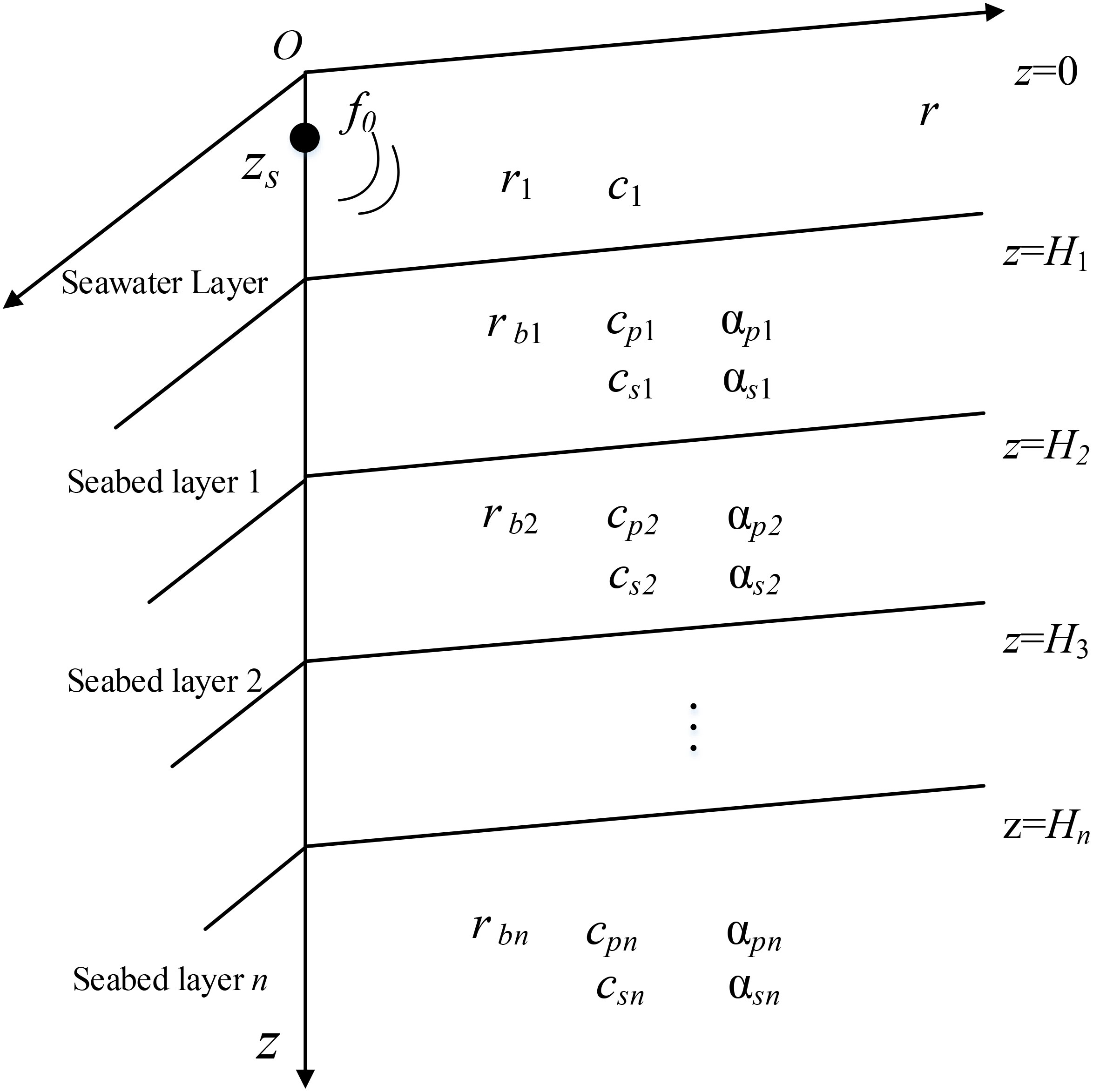
Figure 1 Schematic diagram of the sound field model in cylindrical coordinates.
In the model, it is assumed that the seafloor is regarded as the superposition of n layers of sediments, and the depth of seawater layer is set as H1. The sound source with frequency f0 is located at zs depth of seawater layer. The density and sound velocity in seawater layer are ρ1 and c1, respectively. The depth of the sedimentary layer n is denoted by hn, and the longitudinal wave sound velocity, shear wave sound velocity, density, longitudinal wave sound velocity attenuation and shear wave sound velocity attenuation of the sedimentary layer are denoted by cpn、csn、ρbn、αpn、αsn respectively. The above 6 types of parameters are the submarine acoustic parameters to be retrieved in this study. Under the wave theory, each physical quantity in the above model can be represented by the displacement potential function ϕ. ϕ1 is the displacement potential function of seawater layer. And the research object of this article sound pressure meets p=ρ1ω2ϕ1 (angular frequency ω=2πf0), can be obtained by solving the displacement potential function of fluid, the sound pressure values at various points in the detailed theoretical derivation see literature (Li et al., 2019). Since the displacement potential function in the seawater layer satisfies formula 1 as follows:
The sediments of potential function ϕn can be represented as follows:
Where δ(r,z) is the original function, k represents the wave number of each seafloor, where k=ω/cm, ω=2πf0, pn and sn are the uncertainties contained in the solution, The flow function and potential function of ϕ and ψ correspond to pn and sn respectively. Then the formal solution of formula 2 is as follows:
Where Z is the ordinary differential formula of depth z and ξ of horizontal wavenumber, J0 is the zero-order Bessel function. According to the derivation results of formula 3, the sound pressure field in the water layer can be expressed as follows::
For the solution of formula (4), the Normal Mode Method (NMM) and Fast Field Method (FFM) can be used to solve formula (4). For shallow sea environments, FFM converts the integral formula in formula (4) into Fourier transform form for the direct solution, which is more suitable for fast calculation of sound field in shallow sea (Frederick et al., 2020). Therefore, FFM is selected in this study to conduct a forward simulation of the sound pressure field in the above parametric model.
2.2 BPNN inversion model of geoacoustic parameters inversion
Due to the complexity of the marine environment, factors such as sediment layer density, porosity, and average particle size can all influence acoustic parameters. Consequently, establishing a precise functional relationship between acoustic parameters and shallow water acoustic pressure fields presents a significant challenge. To address this challenge, a non-linear mapping approach utilizing a BPNN is employed (Van Komen et al., 2020). On the other hand, the BPNN is capable of approximating functions through the training of input and output vectors. When feature vectors are input into the network, they can produce results that closely approximate the desired output values. BPNN are a type of multi-layer feedforward neural network that employs both forward signal propagation and backward error propagation to adjust weights and thresholds to minimize the error function value. This iterative process ensures that the modified network output aligns closely with the desired output values (Xu and Pan, 2018).
Therefore, in response to the challenge of inverting seabed bottom properties in the presence of uncertain seabed sediment layering, a method utilizing a BPNN based on shallow water acoustic pressure field data is proposed. Given the inherent coupling between acoustic parameters and the potential for multi-valued solutions, especially in multi-layer seabed environments, training a single neural network directly poses the risk of convergence issues and encounters difficulties due to the vast search space (Zhou et al., 2019).
To address such complexities, this study employs a staged supervised learning approach for multi-layer seabed acoustic parameter inversion. The stepwise seabed layering and parameter inversion process is depicted in Figure 2A. It involves feeding preprocessed and standardized acoustic pressure signals into the NET-1 network, which serves as a classifier for segregating shallow water acoustic pressure data into various seabed layer categories. Based on the classification outcomes, the data is directed to different networks, facilitating targeted acoustic parameter inversion. To accommodate current computational capabilities and practical requirements, this paper primarily discusses scenarios involving seabed layering, specifically semi-infinite seabed (NET-2-1), single sediment layer (NET-2-2), and double sediment layers (NET-2-3). In cases where NET-1 classifies the acoustic pressure data as originating from a single sediment layer, the data is subsequently input into the NET-2-2 network for further acoustic parameter inversion. NET-1 is designed as a single-label classifier solely for layer categorization, without any data alteration. The BPNN models employed for layer categorization in semi-infinite seabed, single sediment layer, and double sediment layer environments are denoted as NET-2-X, where X represents the specific environment (X=1, 2, 3). In total, four BPNN models are trained (Qian et al., 2019).

Figure 2 Schematic diagram of seabed stratification and parameters inversion calculation based on BPNN model: (A) Flow diagram; (B) BPNN (NET 2-1) model.
In the two-step inversion process, the objective of the first step is to determine the seabed type by initially inputting acoustic pressure data into the NET-1 network. The NET model is constructed using a single hidden layer, where neurons within the same layer are not interconnected. In forward propagation, the activation function f(x) links the input signal - acoustic pressure field data pj(ri, zi) - with the hyperparameter matrix [w, b]. The activation function f(x) selected is the Sigmoid function. The signal flows forward from the input layer to the output layer, with w=[wkv, wvl] where wkv represents the weight from the input layer to the hidden layer, and wvl represents the weight from the hidden layer to the output layer (Stoll and Kan, 1981). Additionally, bv signifies the threshold for each neuron in the hidden layer. The backward feedback signal is the error signal E, when the error falls within the predetermined range, network training is terminated. The experimental setup precision is set to 10-3. which reflects the discrepancy between the network model’s inversion results and the true values. For network training, the cross-entropy function ECE is utilized. The calculation of the cross-entropy function is performed as shown in formula (5). NET-1 functions as a single-label classifier, generating outputs based on the categorization of seabed layering, distinguishing between scenarios such as semi-infinite seabed (NET-2-1), single sediment layer (NET-2-2), and double sediment layers (NET-2-3).
After determining the seabed layering structure, the subsequent step involves the stratified inversion of acoustic parameters. In this second phase, we draw inspiration from the application of matched-field acoustic parameter inversion methods. For varying seabed layering conditions, the acoustic signals are input into dedicated BPNN models associated with shallow-water multi-layered seabed environments, based on the classification results obtained from NET-1. The architecture of the NET-2-X models closely resembles that of the NET model. As an illustration, consider the NET-2-1 model, as depicted in Figure 2B. i set of acoustic pressure data from different receiver positions (ri, zi), where (1≤i≤ I), form the input data, denoted asp= [p1(r1, z1), …, pj(ri, zi), …, pm(rI, zI)]m×I. Corresponding ground sound parameters Y=[cpn, csn, ρbn, αpn, αsn]m×5 are employed as output results for model construction (Zhu et al., 2012).
The number of neurons in each layer can be determined based on formula (6):
Where n represents the number of input layer nodes, which corresponds to the simulated acoustic pressure data points, and α is a constant coefficient.
The partial derivatives of weight parameters between the input set of acoustic pressures, denoted as p, and the hidden layer are represented as Δwjv, while the partial derivatives of weights between the hidden layer and the ground sound parameters Y are represented as Δwvl. The learning rate, η, is employed during the computation. In this process, the iteration step t is continually updated based on whether the EMSE value satisfies the predetermined accuracy. The adjustment of parameters, wjv、wvl is achieved through the modification of weight values, aiming to minimize errors. The parameter descent is carried out using a gradient descent approach (Zhang et al., 2021). The method for modifying parameters wjv and wvl is as follows, as expressed in the (formulas 7, 8).
The assessment of the training network’s effectiveness is based on the Root Mean Square Error (RMSE), as described in formula (9).
Where Yrea,pre=[cp, cs, ρb, αp, αs], a matrix comprising the parameters to be inverted, with Yrearepresenting the simulated values and Yprerepresenting the inverted values.
The sound pressure input undergoes a nonlinear transformation within the network, ultimately resulting in the geophysical parameters (Cheng et al., 2021). In this process, the inputs and outputs of the hidden layer are denoted as Ikvand Ivl, respectively. The final inversion result, Ypre, is computed as shown in formula (10).
To determine an appropriate network structure, this paper simplifies the seafloor into two layers, thus establishing the BPNN inversion model (Zhu et al., 2017). In this model, the input layer receives simulated sound pressure data, denoted as “p,” which includes a set of sound pressure data pj(ri, zi), where the range of i extends from 1 to I. The number of neurons in the hidden layer is set at 9, and this choice is influenced by various factors, one of which is the empirical rule for parameter α, which is set to α = -15 in this context (Zheng et al., 2021). Furthermore, the number of neurons in the output layer, represented as “l,” is determined based on the number of geophysical parameters that need to be inverted. For instance, have lNET-1 = 4, lNET-2-1 = 5, lNET-2-2 = 11, lNET-2-3 = 17.
2.3 Data generation and fitting verification
The equations should be inserted in editable format from the equation editor. Considering the variation range of ground sound parameters in shallow sea (Li et al., 2019), the parameters training range of the BPNN model for ground sound parameters inversion under a preset environment is set as shown in Table 1.
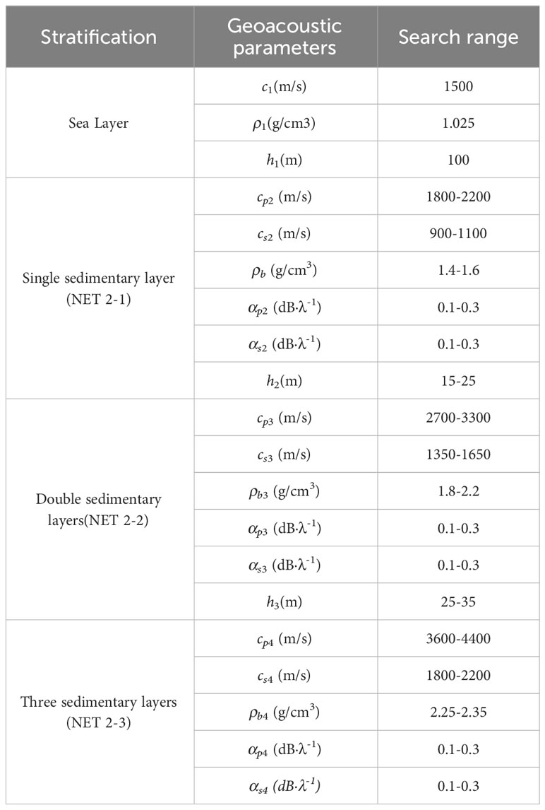
Table 1 BPNN model training set search range.
The simulated sound pressure field data is a set of horizontal equally spaced receiving sound pressure fields under the set sound source depth zs=20m, receiving depth zr=10m and seawater depth H=100m. The receiving points are spaced 2m apart, and a total of I=720 receiving points are set. The model training samples adopted by NET2-X are 2200 groups of sound pressure data randomly generated in each layer within the search range in Table 1, among which 200 groups are randomly divided into training sets and the other 200 groups into test sets. Each group (Layered structure) of the training set and its corresponding environmental sound pressure are mapped into the model one by one for training. When the error function EMSE reaches the set accuracy σ=0.01, the training is completed (Huang et al., 2018).
The verification set is generated using random values. The changes in loss function and prediction accuracy in the training process of NET-1 are shown in Figure 3. As can be seen from Figure 3A, after a certain batch of training, the error of the training curve is reduced to σ, the network stops training, and the confusion matrix further verifies that NET-1 also has a good classification effect on the verification data, and can complete the classification calculation of the submarine stratified structure.

Figure 3 NET-1 training analysis: (A) Loss function; (B) Visual analysis.
In Figure 3B, the inside of each orange box represents the number of incorrectly predicted samples, the main diagonal represents the number of correctly predicted samples, and the light gray rectangle box at the lower right represents the prediction accuracy of the corresponding sample attributes, that is, the accuracy of 95% in the training process.NET 2-X conducts training for neural networks under three hierarchical structures respectively. To enhance the credibility of the model, the Mean Absolute Error (MAE) was introduced as an evaluation metric to assess the predictive accuracy of the model. The calculation results are shown in Table 2. Taking the NET2-1 scenario as an example, a smaller MAE value indicates better predictive capability of the model. The calculated results demonstrate that the inversion error of the model is small, indicating that the BP neural network performs well in the inversion of shallow-sea acoustic parameters. Consequently, the constructed BP neural network model exhibits good and stable predictive performance in the inversion of shallow seabed acoustic parameters, with high computational efficiency and reliability of the prediction results.
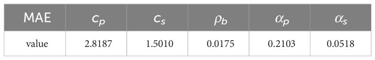
Table 2 NET 2-1Parameter setting of the inversion algorithm.
The changes in loss function in the training process are shown in Figure 4. Taking NET 2-2, which corresponds to the layered structure of the seabed as a single sedimentary layer, as an example, after the completion of training, the EMSE value reached the setting accuracy after 200 iterations. The error reduction process was relatively stable, indicating that the error reduction speed and training effect of the whole neural network in the training is considerable. Although with the increase of inversion parameters, the number of iteration steps to reach the accuracy setting in the NET 2-X training increased, the target accuracy was reached within 500 iterations, which effectively constructed BPNN model that could meet the inversion accuracy of layered submarine acoustic parameters.
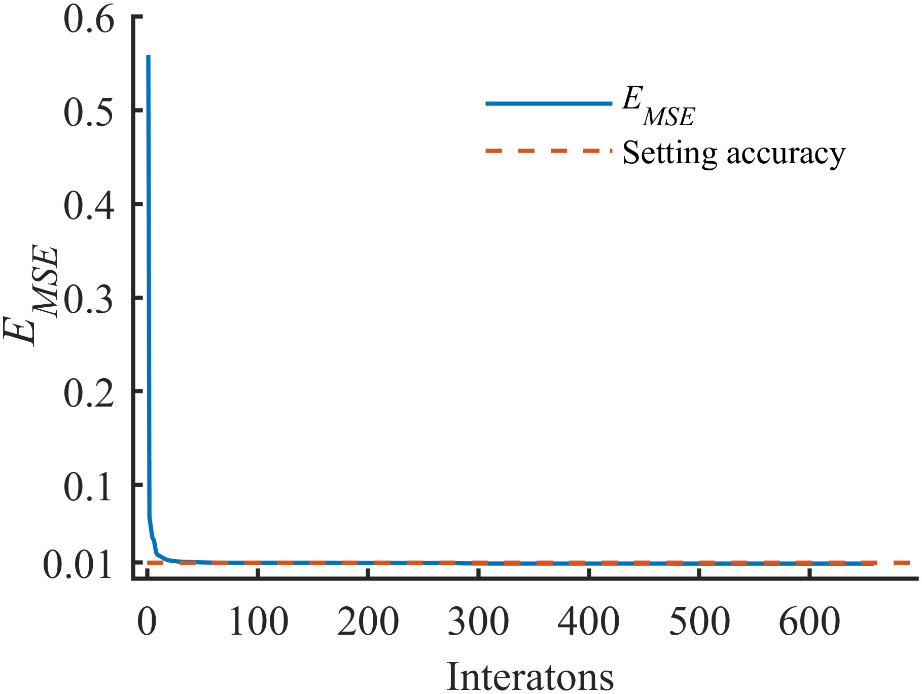
Figure 4 NET 2-2 loss function changes.
By controlling the training parameters and adjusting the training function, the overfitting phenomenon can be eliminated in the process of network training, and the generalization ability of the model can be improved. The highly generalized multi-output model can solve the multi-value problem caused by the coupling relationship between the seabed parameters in the inversion process to some extent, to realize the purpose of simultaneously inverting multiple seabed acoustic parameters.
2.4 Simulation result analysis
Simulation data and experimental data are used to test the performance of BPNN model respectively, and the network prediction results are used in the seabed stratification calculation and earth acoustic parameters inversion of the measured data of the pool (Yu et al., 2020).
As a classification model, NET-1 can be directly evaluated based on the classification accuracy of the test set, as shown in formula (11).
Where, Nt is the number of correct samples for stratification and N= m-Mt, which is the number of total test samples. As a regression analysis problem, to quantify the error between the inversion results of each parameters and the preset truth value, the performance function R2 was introduced to represent the coincidence degree between the inversion value and the true value numerically. The closer the R2 value was to 1, the closer the inversion result was to the preset truth value (Zhang, 2023). The calculation method is shown in Formula 12.
To verify the robustness of the training completion network, the sound pressure of the test set generated within the search interval and some environmental noise are added as test data. The total number of samples in the test set is 10% of the training set.
Figure 5 shows the layering results of NET-1 on part of the test set. The layering accuracy Ea=99% proves that NET-1 can effectively perform layering calculations on sound pressure field information under different layering structures. In the figure, “x” represents the predicted value, “o” represents the true value, and the Y-axis represents the search range of the number of hierarchical structures.
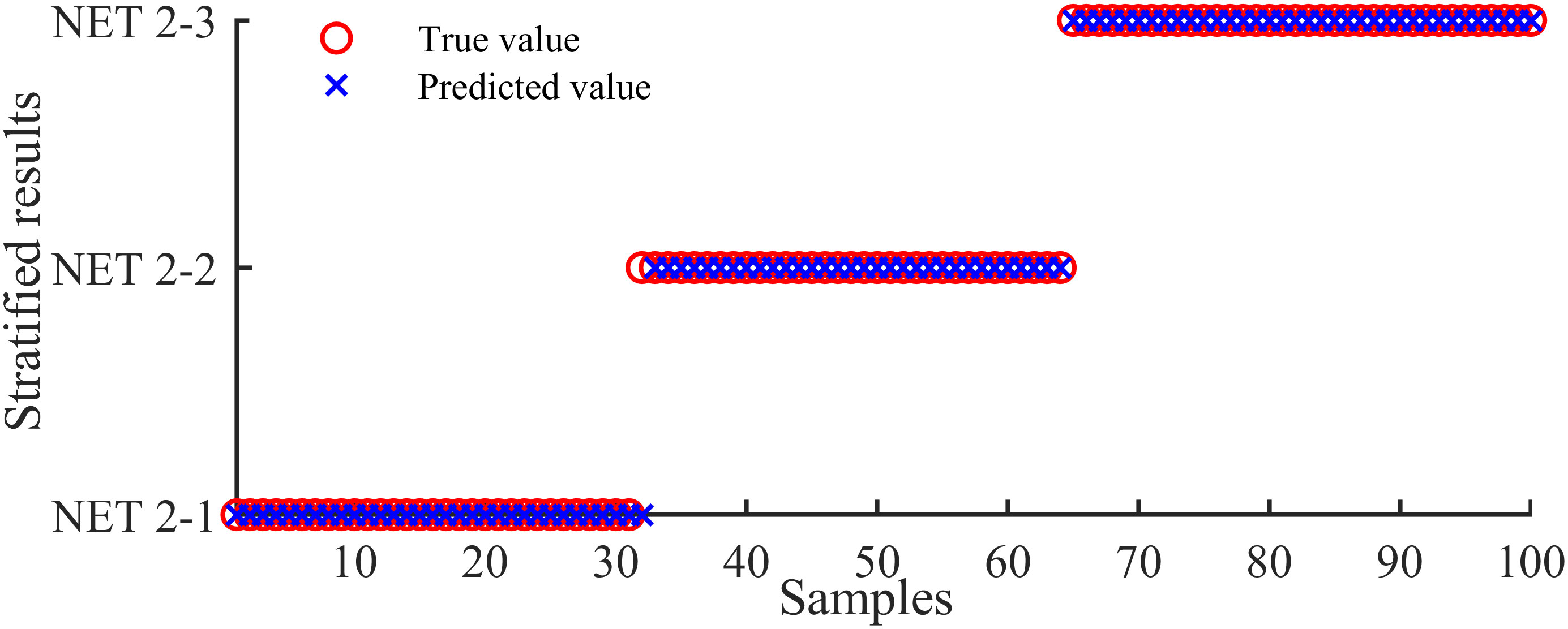
Figure 5 Seabed stratification results of NET-1.
At the same time, the NET 2-X model is trained. Taking NET 2-2 as an example, Figure 6 shows the results of underwater acoustic parameters inversion of NET 2-2. The solid line and “×” in the figure correspond to the real value and predicted value of the test data set respectively.
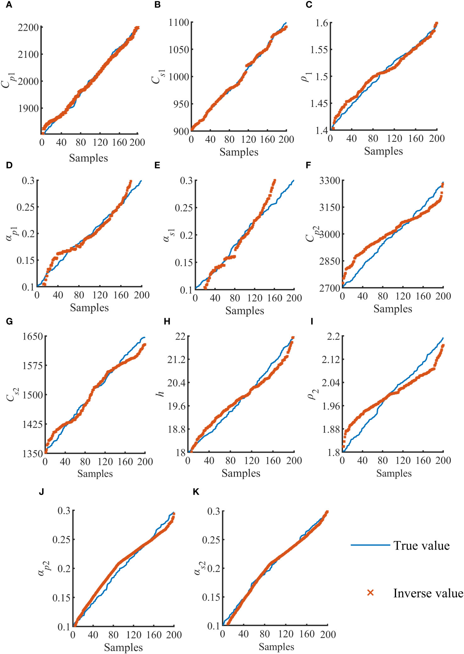
Figure 6 NET-2-2 Comparison between the actual and predicted values of 200 samples of single sediment. (A–K) are inversion results of 11 parameters in the case of NET 2-2, respectively.
Figure 6 shows the degree of fitting between the predicted value and the preset value of each parameter in the test set in the inversion model. During verification, the fitting degree of the inversion results of cpn, csn, ρbn, and hn is maintained above 0.90, showing an excellent inversion effect. The error variation of parameters αpn and αsn is relatively large, but the R2 value of each parameter is above 0.80, The overall error appears to be within acceptable limits. It can be seen that the BPNN model constructed has good and stable prediction performance for shallow sea floor acoustic parameters inversion, and the prediction results have high reliability.
Figures 6A–F shows the ground sound parameter training results of the first sedimentary layer, and Figures 6G–K shows the ground sound parameter training results of the second sedimentary layer. As can be seen from the figure, the training effect of the first layer is better and the degree of fitting is higher. It can be seen from the literature that different parameters have different influences on acoustic propagation characteristics, especially cpn and csn have the greatest influence on acoustic field characteristics, so the accuracy of inversion results of these parameters is higher than other parameters. From the fitting degree in the training process, it can be seen that the fitting degree of cpn and csn parameters is better, which accords with the law of sound field calculation in the forward modeling model, which proves the applicability of the method.
A group of sound pressure data with a single true value is used for inversion calculation. Substitute the true value sound pressure data into the neural network models, and the classification results are shown in Table 3. It can be seen from Table 3 that the classification probabilities of Net 2-X model for the seabed layered structure under the true sound pressure are: X=1, rate=1.21×10⁻³; X=2, rate=0.99; X=3, rate=1.52×10⁻⁴,The data is determined to be acoustic pressure data from a two-layer seabed.
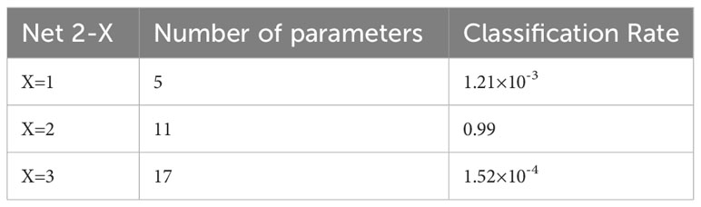
Table 3 Prediction results of Net 2-X.
After determining the bottom stratification structure, The input data will be brought into the corresponding neural network model Net 2-X for inversion calculation and the acoustic parameters inversion values are shown in Table 3. To verify the correctness of hierarchical judgment, the sound field calculation model at X= 1,2 and 3 is used for inversion discussion and comparison with X=2 respectively. Figure 7 shows the comparison between the Transmission Loss (TL) curve calculated by setting the truth value of acoustic parameters and the TL curve calculated by using inversion results. It can be seen from the comparison that the distribution characteristics of the two curves are consistent, which further proves the accuracy of the inversion results of the subsurface acoustic parameters of the preset model based on BPNN model (Yang, 2023).
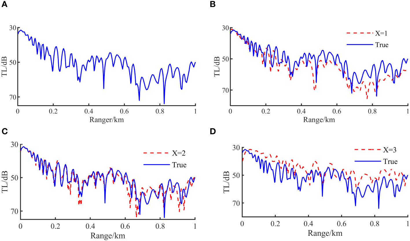
Figure 7 Comparison between X=2 simulated TL curve and X=1, 2, 3inversion TL curve: (A) TL curve under true value; (B) Comparison of TL curves of Net 2-1 models and true value. (C) Comparison of TL curves of Net 2-2 and true value. (D) Comparison of TL curves of Net 2-3 and true value.
Combining the classification results in Table 3, the parameters inversion results in Table 4 and the comparison of TL curves under the three hierarchical structures in Figure 8, the above results show that when the actual model matches the inversion model exactly the prediction is X=2, which proves that the model is the best-parameterized model. At the same time, the TL comparison obtained by the inversion parameters of the X=1, 2, and 3 models also proves the above conclusion. When X=2, the parameters inversion results in Table 4 are consistent with the present. The above simulation results prove that this method can theoretically achieve accurate inversion of seabed layered structures and seabed geoacoustic parameters.
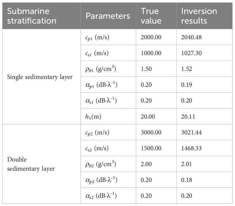
Table 4 Simulation parameters setting and search range.
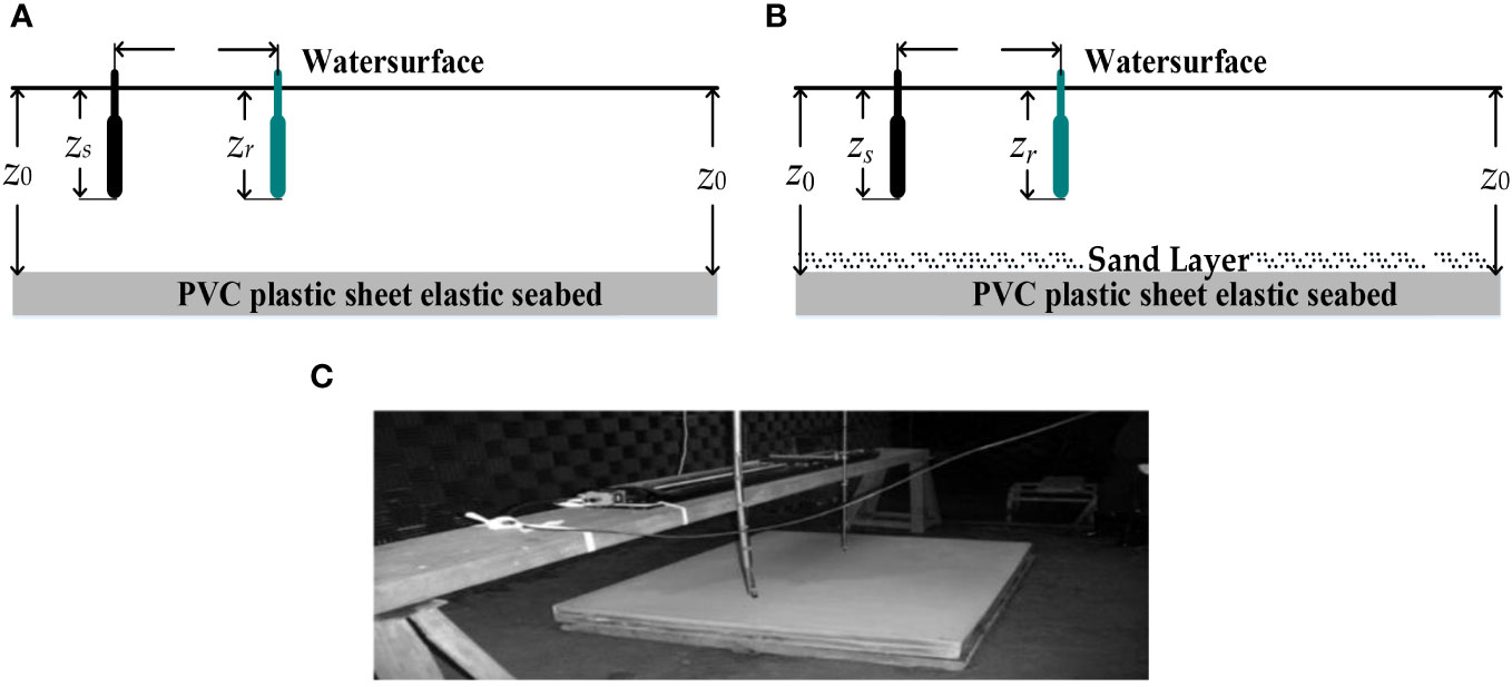
Figure 8 The equipment in the experiment: (A) Schematic diagram of the experiment under a single sedimentary layer (PVC); (B) Schematic diagram of the experiment under a double sedimentary layer (PVC+sand); (C) Experimental equipment layout physical map.
3 Measurements and results
3.1 Introduction of experiment
Previous studies have shown that, under the assumption that various acoustic parameters in waveguides are unchanged, the idea of equal ratio can be used to simulate the acoustic propagation test in the actual ocean by using the equal ratio of high-frequency sound sources in the laboratory, and the expression only changes the ratio, while the propagation characteristics of the sound field remain unchanged. Based on simulation verification of the accuracy and applicability of the proposed method, the feasibility of the proposed inversion method in practical application is further verified in this section combined with the experimental data of the muffler pool shrinkage. The experiment was carried out in a hydrating pool, using a uniform and high-hardness polyvinyl chloride (PVC) plate (the density of PVC was 1.20g/cm-3) as a “semi-infinite elastic seabed”.
To verify the applicability of the inversion method, two schemes were adopted in the experiment as follows:
1. There is only PVC plate, simulating elastic semi-infinite seabed.
2. The way of laying fine sand on PVC plate simulates the shallow sea waveguide environment with a single layer of elastic sediment and an elastic version of the infinite seabed, and the thickness of the sediment simulated by fine sand is about 250 mm.
Only the stratification of the sea floor was different between the two schemes, and other experimental factors were consistent. The layout of experimental equipment 1 is shown in Figure 8A, The other is shown in Figure 8B. The depth of the sound source and the receiving hydrophone are set to 200mm, and the depth of the fluid layer is 300mm. The speed of sound calculated in the laboratory at room temperature is 1450.212 m·s-1. High-frequency underwater sound waves are transmitted by a fixed location sound source at a frequency of 155KHz and received by a single TC4038 standard hydrophone at different locations at equal intervals. To improve the measurement accuracy, a high-precision controllable moving platform was selected to limit the error within 2um and the unit accuracy was 2mm. A total of 500 position points were measured during the experiment. Each position was measured 10 times and the average value was taken as the final test data.
3.2 Model selection and inversion results
The computational process of the acoustic field measured under two experimental schemes is illustrated in Figure 2A. Initially, the layered structure is assessed using NET-1. The types of input data include semi-infinite seabed and two-layer seabed, with the layering results depicted in Figure 9, presented in the form of probabilities. It is observed that the NET-1 model’s probabilistic assessment for the two input acoustic pressure signals as semi-infinite seabed and single sediment seabed is 99%, consistent with the scale model experiments. Additionally, a comparison between the simulated annealing algorithm and the classical annealing algorithm was conducted, incorporating the respective NET 2-X (X=1,2) models.
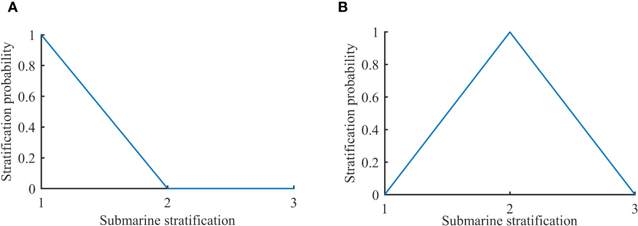
Figure 9 Judgment of two types of layered seabed structures: (A) NET2-1 judgment for semi-infinite seabed layering, (B) NET2-2 judgment for two-layer seabed stratification.
The inversion results obtained by BPNN and SA are shown in Table 5. In the pool experiment, PVC boards with a density of 1.20 g/cm³ were used to simulate the seabed layer, and the thickness of the fine sand layer, representing the sediment layer, was set to 250 mm. Utilizing the data acquired from the pool experiment, the Back Propagation Neural Network (BPNN) inversion results indicated the simulated seabed layer density to be 1.23 g/cm³, and the inferred thickness of the sediment layer to be 251.13 mm. The relative errors were found to be 2.5% and 0.51%, respectively, demonstrating good accuracy of the inversion process. In addition, the inversion results obtained in this paper are compared with those obtained from PVC plates simulating the same material of semi-infinite seabed. The velocity of P-wave and S-wave in the semi-infinite seabed is 2399.364 m/s and 1242.978 m/s. The relative error is controlled below 5%.
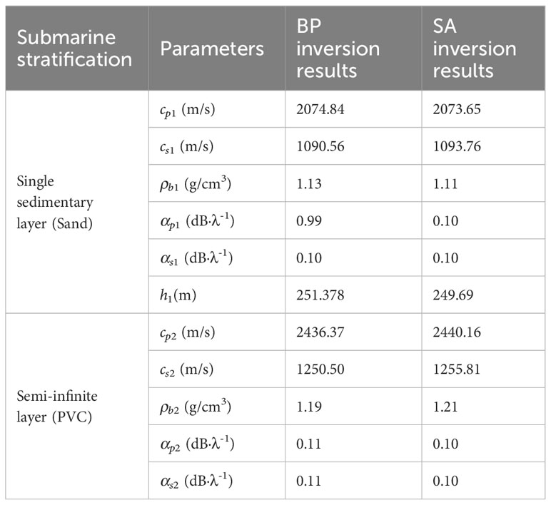
Table 5 Scheme 2 inversion results of measured data.
Considering the coupling effect of multiple parameters, to further verify the accuracy of inversion, the comparison between the dispersion curve of BPNN inversion and the measured dispersion curve is shown in Figure 10. And under the two experimental schemes, the comparison curve of propagation loss between BPNN model and SA inversion algorithm on measured data is shown in Figure 11.
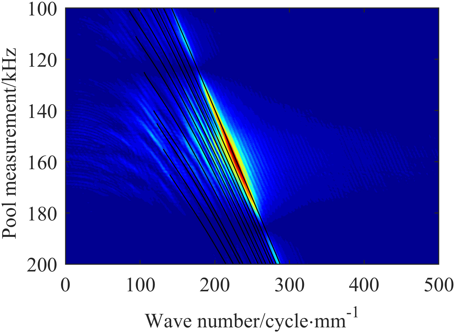
Figure 10 Comparison between BP inversion and measured dispersion curve.
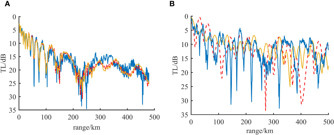
Figure 11 BP and SA inversion TL curve compared with measured TL: (A) Comparison diagram of TL curve under experimental scheme 1; (B) Comparison of propagation loss curves under experimental scheme 2ganxie.
Figure 10 shows the frequency-wave number spectrum measured by the water tank. It can be seen from the spectrum that the energy of the received sound pressure signal is mainly distributed in the range of 145kHz-175kHz, and its peak value is around 155kHz, which is consistent with the performance index of the sound source set in the experiment. In order to verify the effectiveness of the BPNN inversion approach and to compare the TL computed from the inversion results for both semi-infinite and two-layer seabed configurations with the TL measured in scale-down experiments, the following findings were observed: For the semi-infinite single-layer seabed scenario, the TL was generally consistent. In the case of the two-layer seabed, taking into account various uncertainties such as the replacement of the sediment layer with fine sand and the homogeneity of the sand, certain discrepancies were observed. However, the overall trend of the TL was closely aligned. This demonstrates that the inversion method proposed in this article yields results for the inversion of parameters such as longitudinal wave and shear wave velocities in multi-layer seabed structures that are in substantial agreement with the actual data.
3.3 Result analysis¿
Geoacoustic parameters inversion is a nonlinear and multi-parameter optimization problem, so the inversion results obtained by different inversion methods are not the same, but all have the same reliable reference value. The coupling of multiple parameters often leads to the experimental phenomenon of the same result in different parameters combinations, so it is necessary to discuss the sensitivity of different parameters to determine the reference weight of the choice of results.
The applicability of multi-parameter inversion using BPNN can be obtained from spectrum analysis and comparison with SA algorithm. From the comparison and verification of TL curves of the two experiments, it can be seen that when the seafloor structure is inversion for single-layer, the inverse performance results of BPNN and SA algorithm have higher accuracy; when the seafloor is inversion for double-layer seafloor, the number of ground acoustic parameters increases, the inversion difficulty increases, and the multi-parameter coupling is enhanced, so there is a relatively obvious deviation. However, in terms of the inversion results of the two algorithms, the root mean square error of the TL curve obtained by the experiment is 121.92 and 160.19, respectively, compared with that of BPNN TL curve and SA TL curve. Relatively speaking, the error of the inversion results of BPNN is smaller and more valuable for reference.
4 Conclusions
By employing the BPNN inversion method to train an extensive dataset of simulated information, a computational model has been established with the capability to effectively evaluate the stratified structure of the seabed along with its acoustic parameters. Within this study, the BPNN inversion algorithm has been applied to the inversion of Earth’s acoustic parameters, thus contributing to the advancement of fields in geophysics and ocean acoustics. This approach holds significant promise for practical applications in the realms of seabed resource exploration, ocean environmental investigations, marine engineering, and the exploitation of ocean resources, among others.
Our research findings can be succinctly summarized as follows:
The Fast Field Method (FFM) was utilized to derive theoretical predictions for the shallow-sea sound pressure field. Subsequently, a model was established within the BPNN framework, connecting the predicted sound pressure field with the underlying acoustic parameters. The measured sound pressure field data were then processed through the neural network model to obtain inversion results. Both simulated and experimental data confirm the accuracy of this proposed method in retrieving geoacoustic parameters.
The acoustic pressure field in water is influenced by five crucial acoustic parameters associated with shallow seabed conditions: bottom density, p-wave velocity, S-wave velocity, p-wave velocity attenuation, and S-wave velocity attenuation. Our results reveal that the accuracy of the inversion results for S-wave velocity (cp), p-wave velocity (cs), and sedimentary layer density (ρb) surpasses that of S-wave attenuation (αp) and p-wave attenuation (αs). The first three acoustic parameters exert a more pronounced impact on the propagation characteristics of the shallow-sea sound pressure field, thus demonstrating a more apparent correlation with the acoustic pressure data. This further illustrates the effectiveness of employing the BPNN model for inversion in the context of shallow seabed layering.
Given the practical complexities of shallow seabed conditions, compounded by the influence of various underwater noises on sound field distribution, actual computational results may exhibit some deviation from real-world scenarios. Additionally, the coupling relationships between seabed physical parameters and the sensitivity of each parameter can impact calculation accuracy. To address these limitations, we have optimized the BPNN model by adjusting its neural network structure and introducing random noise in subsequent research, thus enhancing the reliability of the Earth’s acoustic parameter inversion model. Moreover, we have conducted an exhaustive exploration and discussion concerning the impact of network configuration parameters on the accuracy of inversion results.
These revisions are aimed at addressing the reviewer’s concerns and enhancing the clarity and impact of the conclusion section.
Data availability statement
The original contributions presented in the study are included in the article/supplementary material. Further inquiries can be directed to the corresponding authors.
Author contributions
JW: Conceptualization, Data curation, Methodology, Writing – original draft, Writing – review & editing. ZC: Conceptualization, Data curation, Methodology, Writing – original draft. HZ: Methodology, Validation, Writing – review & editing. LM: Formal analysis, Supervision, Writing – review & editing. WS: Funding acquisition, Project administration, Resources, Writing – review & editing. XL: Investigation, Methodology, Writing – original draft.
Funding
The author(s) declare financial support was received for the research, authorship, and/or publication of this article. This research was funded by the National Natural Science Foundation of China (Grant No: 12374425), the Stable Supporting Fund of the National Key Laboratory of Underwater Acoustic Technology (JCKYS2023604SSJS016), the Science and Technology program of Zhoushan City (2023C41025), the Fund of Fujian Provincial Key Laboratory of Marine Physical and Geological Processes (KLMPG-23-01) and the Zhejiang University Student Science and Technology Innovation Program (New Miao Talent Program) (2022R411C050, 2022R411C052).
Conflict of interest
Author ZC was employed by the company Hydroacoustics Technology Co., Ltd.
The remaining authors declare that the research was conducted in the absence of any commercial or financial relationships that could be construed as a potential conflict of interest.
Publisher’s note
All claims expressed in this article are solely those of the authors and do not necessarily represent those of their affiliated organizations, or those of the publisher, the editors and the reviewers. Any product that may be evaluated in this article, or claim that may be made by its manufacturer, is not guaranteed or endorsed by the publisher.
References
Chen J.-H., Chen L.-P., Xia X.-Y., Zhu R. (2022). Classification of submarine sonar images based on transfer learning. Comput. Simul. 39, 229–233.
Cheng X. U. E., Zaixiao G., Yiming G. U., Yu W., Peng L. I. N., Zhenglin L. I. (2021). Channel matching of shallow water active detection combined with convolutional neural network. Acta ACUSTICA 46 (6), 800–812. doi: 10.15949/j.cnki.0371-0025.2021.06.003
Dragna D., Blanc-Benon P. (2017). Sound propagation over the ground with a random spatially-varying surface admittance. J. Acoust. Soc. Am. 142 (4), 2058–2072. doi: 10.1121/1.5006180
Feng X., Zhou M., Zhang X., Ye K., Wang J., Sun H. (2022). Variational bayesian inference based direction of arrival estimation in presence of shallow water non-gaussian noise. J. Electron. Inf. Technol 44(6), 1887–1896. doi: 10.11999/JEIT211284
Frederick C., Villar S., Michalopoulou Z.-H. (2020). Seabed classification using physics-based modeling and machine learninga). J. Acoust. Soc. Am. 148 (2), 859–872. doi: 10.1121/10.0001728
Gerstoft P. (1994). Inversion of seismoacoustic data using genetic algorithms and a posteriori probability distributions. J. Acoust. Soc. Am. 95 (2), 770–782. doi: 10.1121/1.408387
Huang Z., Xu J., Gong Z., Wang H., Yan Y. (2018). Source localization using deep neural networks in a shallow water environment. J. Acoust. Soc. Am. 143 (5), 2922–2932. doi: 10.1121/1.5036725
Ke Q. U., Changqing H. U., Mei Z. (2013). Single parameter inversion using transmission loss in shallow water. Acta ACUSTICA 38 (4), 472–476. doi: 10.15949/j.cnki.0371-0025.2013.04.017
Kerzhakov B. V., Kulinich V. V. (2016). Retrieval of sea-bed parameters by the method of matching acoustic fields on the basis of vertical angular spectra. Radiophysics Quantum Electron. 59 (3), 217–224. doi: 10.1007/s11141-016-9690-x
Li H., Guo X.-Y., Ma L. (2019). Estimating structure and geoacoustic parameters of sub-bottom by using spatial characteristics of ocean ambient noise in shallow water. Acta Physica Sin. 68 (21), 214303–214301-214303-214312. doi: 10.7498/aps.68.20190824
Li R., Zhang H., Zhuang Q., Li R., Chen Y. (2020). BP neural network and improved differential evolution for transient electromagnetic inversion. Comput. Geosci. 137, 104434. doi: 10.1016/j.cageo.2020.104434
Li X., Piao S., Zhang M., Liu Y. (2019). A passive source location method in a shallow water waveguide with a single sensor based on bayesian theory. Sensors 19 (6), 1452. doi: 10.3390/s19061452
Li Z., Zhang R. (2017). Hybrid geoacoustic inversion method and its application to different sediments. J. Acoust. Soc. Am. 142 (4_Supplement), 2558–2558. doi: 10.1121/1.5014351
Pang Y., Xu F., Liu J. (2021). Classification of seafloor sediment based on Gammatone Filter banks time Spectrum and Convolutional Neural networks. Appl. Acoust. 40 (04), 510–517. doi: 10.11684/j.issn.1000-310X.2021.04.003
Potty G. R., Miller J. H., Dosso S. E., Bonnel J., Dettmer J., Isakson M. J. (2017). Sediment parameter inversions in the East China Sea. J. Acoust. Soc. Am. 141 (5_Supplement), 3487–3487. doi: 10.1121/1.4987270
Qian G., Zhang L., Wang Y. (2019). Single-label and multi-label conceptor classifiers in pre-trained neural networks. Neural Comput. Appl. 31 (10), 6179–6188. doi: 10.1007/s00521-018-3432-2
Song W., Wang P. (2022). High-resolution modal wavenumber estimation in range-dependent shallow water waveguides using vertical line arrays. J. Acoust. Soc. Am. 152 (1), 691–705. doi: 10.1121/10.0012187
Stoll R. D., Kan T. K. (1981). Reflection of acoustic waves at a water–sediment interface. J. Acoust. Soc. Am. 70 (1), 149–156. doi: 10.1121/1.386692
Van Komen D. F., Neilsen T. B., Howarth K., Knobles D. P., Dahl P. H. (2020). Seabed and range estimation of impulsive time series using a convolutional neural network. J. Acoust Soc. Am. 147 (5), El403. doi: 10.1121/10.0001216
Wang Z.-J. (2008). Inversion of seabed parameters for vertical array (Harbin Engineering University). Master.
Wang J., Cao J.-X., Zhao S., Qi Q.-M. (2022). Inverse prediction method of shear wave velocity based on deep hybrid neural network. Scientia Sin. Terrae 52, 1151–1169. doi: 10.1360/SSTe-2021-0128
Wang Z., Ma Y., Kan G., Liu B., Zhou X., Zhang X. (2023). An inversion method for geoacoustic parameters in shallow water based on bottom reflection signals. Remote Sens. 15 (13), 3237. doi: 10.3390/rs15133237
Wen B.-Y., Tang W.-C., Tian Y.-W. (2021). Significant wave height field inversion of high frequency radar based on BP neural net-work. J. Huazhong Univ. Sci. Technol. 49 (4), 114–119. doi: 10.13245/j.hust.210420
Xu Y.-Y., Pan X. (2018). Research on passive geoacoustic inversion. J. Hangzhou Dianzi Univ. (Nat. Sci. Ed.). 38, 45–49.
Xue Y., Zhu H., Wang X., Zheng G., Liu X., Wang J. (2023). Bayesian geoacoustic parameters inversion for multi-layer seabed in shallow sea using underwater acoustic field. Front. Mar. Sci, 10. doi: 10.3389.2023/fmars.1058542
Yang P. (2023). An imaging algorithm for high-resolution imaging sonar system. Multimedia Tools Appl., 1–17. doi: 10.1007/s11042-023-16757-0
Yang L.-F., Zhu Z.-R., Li J.-B., Feng C.-K. (2021). Seafloor classification based on combined multibeam bathymetry and backscatter using deep convolution neural network. Acta Geod. Cartogr. Sin. 50, 71–84. doi: 10.11947/J.AGCS.2021.20200065
Yu S.-Q., Wang F., Zheng G.-Y. (2020). Progress and discussions in acoustic properties of marine sediments. J. Harbin Eng. Univ. 41, 1571–1577. doi: 10.11990/jheu.202007049
Zhang X. (2023). An efficient method for the simulation of multireceiver SAS raw signal. Multimedia Tools Appl., 1–18. doi: 10.1007/s11042-023-16992-5
Zhang X., Wu H., Sun H., Ying W. (2021). Multireceiver SAS imagery based on monostatic conversion. IEEE J. Selected Topics Appl. Earth Observations Remote Sens. 14, 10835–10853. doi: 10.1109/JSTARS.2021.3121405
Zhao Y., Zhu K., Zhao T., Zheng L., Deng X. (2023). Small-sample seabed sediment classification based on deep learning. Remote Sens. 15 (8), 2178. doi: 10.3390/rs15082178
Zheng G.-X., Piao S.-C., Zhu H.-H. (2021). Bayesian inversion method of geo-acoustic parameters in shallow sea using acoustic pressure field. J. Harbin Eng. Univ. 42, 497–504. doi: 10.3390/s20072150
Zhou J., Zhang M., Piao S., Iqbal K., Qu K., Liu Y., et al. (2019). Low frequency ambient noise modeling and comparison with field measurements in the South China Sea. Appl. Acoust. 148, 34–39. doi: 10.1016/j.apacoust.2018.11.013
Zhu H., Cui Z., Liu J., Jiang S., Liu X., Wang J. (2023a). A method for inverting shallow sea acoustic parameters based on the backward feedback neural network model. J. Mar. Sci. Eng. 11 (7), 1340. doi: 10.3390/jmse11071340
Zhu H.-H., Hai-Gang Z., Wei L. (2013). Research on the influence of sound speed profile to the dispersion in shallow water waveguide. Tech. Acoust. 32, 67–68.
Zhu H.-H., Piao S., Zhang H., Liu W., An X. (2012). The research for seabed parameters inversion with fast field program (FFP). J. Harbin Eng. Univ. 33, 648–652+659. doi: 10.3969/j.issn.1006-7043.201105075
Zhu H., Xue Y., Ren Q., Liu X., Wang J., Cui Z., et al. (2023b). Inversion of shallow seabed structure and geoacoustic parameters with waveguide characteristic impedance based on Bayesian approach. Front. Mar. Sci. 10. doi: 10.3389/fmars.2023.1104570
Keywords: seabed stratification, acoustic parameters inversion, BPNN, fast field method (FFM), scale test
Citation: Wang J, Cui Z, Zhu H, Meng L, Song W and Liu X (2024) A back propagation neural network-based approach for inverting layered seabed acoustic parameters in shallow waters. Front. Mar. Sci. 11:1349478. doi: 10.3389/fmars.2024.1349478
Received: 04 December 2023; Accepted: 26 January 2024;
Published: 28 February 2024.
Edited by:
Xuebo Zhang, Northwest Normal University, ChinaReviewed by:
Hiroyuki Matsumoto, Japan Agency for Marine-Earth Science and Technology (JAMSTEC), JapanChuanxi Xing, Yunnan Minzu University, China
Jia Liu, Chinese Academy of Sciences (CAS), China
Copyright © 2024 Wang, Cui, Zhu, Meng, Song and Liu. This is an open-access article distributed under the terms of the Creative Commons Attribution License (CC BY). The use, distribution or reproduction in other forums is permitted, provided the original author(s) and the copyright owner(s) are credited and that the original publication in this journal is cited, in accordance with accepted academic practice. No use, distribution or reproduction is permitted which does not comply with these terms.
*Correspondence: Hanhao Zhu, emh1a2xtcGdAMTYzLmNvbQ==; Weihua Song, d2hzb25nQHpqb3UuZWR1LmNu
†These authors have contributed equally to this work and share first authorship