 Yundong Li
 Guijun Han*
 Xiaobo Wu
 Lige Cao
- Tianjin Key Laboratory for Marine Environmental Research and Service, School of Marine Science and Technology, Tianjin University, Tianjin, China
Introduction: Salinity is a key variable in the dynamic and thermal balance of the entire climate system. To address the complexities of diverse terrains and fluctuating ocean waves, we commonly use free-surface models with quasi-stationary (e.g. height, pressure, or terrain following) coordinates for simulating salinity. In such models, the vertical grid dynamically adjusts with the undulation of seawater. However, this adjustment also occurs when freshwater enters or exits the ocean. Freshwater-induced salinity changes at the ocean’s surface are artificially distributed to each vertical layer within a model time step. This means that the freshwater at the ocean surface instantaneously and directly affects the seafloor. This process is different from physical diffusion processes. The diffusion effects caused by the influx and outflow of freshwater have a very small impact on the seafloor. This error leads to salinity non-conservation and disrupts the vertical distribution structure of salinity. Previous studies have also addressed this issue with solutions such as the vertical Lagrangian-remap method.
Method: This paper proposes a natural vertical distribution calculation scheme (NVDCS) which is different from the approaches of our predecessors. In the discrete formulation of the original ocean equations, freshwater flux is introduced to ensure salinity conservation. In each model time step, by calculating the seawater volume changes due to freshwater inflow or outflow, as well as the vertical grid changes caused by sea surface undulations, the aforementioned artificial error is eliminated from each vertical layer.
Discussion: This scheme ensures that changes in the vertical coordinates of each layer result solely from internal oceanic dynamic processes, avoiding the instantaneous and directly impact of surface freshwater. Ultimately, the influence of freshwater is confined to the ocean surface.
Results: This method is straightforward to implement and user-friendly. Sensitivity experiments indicate that in free-surface models, quasi-stationary coordinates introduce artificial errors. The proposed calculation scheme not only eliminates this error but also achieves a better vertical distribution structure than using virtual salt flux, while ensuring salinity conservation.
1 Introduction
Salinity is one of the most crucial indicators in studying the physical properties and dynamic mechanisms of the ocean (Garcia-Soto et al., 2021). It dictates the density and circulation of the ocean, thereby influencing the entire climate system (Vialard and Delecluse, 1998). Before the year 2000, ocean numerical models commonly used virtual salt flux or relaxation conditions as boundary conditions for salinity simulation. While such conditions visually enhanced the apparent reasonableness of salinity distribution, they resulted in non-conservation of salt. Subsequently, the introduction of real freshwater flux successfully extended to free-surface ocean models, addressing to the conservation of salinity. The significance of freshwater forcing has been demonstrated to be equal to that of heat forcing, wind stress, etc., impacting the state of the ocean and playing a crucial role in the formation of the Goldsbrough-Stomme circulation (Huang, 1993; Oka and Hasumi, 2004). Typically, freshwater forcing from processes like evaporation, precipitation, and runoff can only directly impact the surface layer of seawater (Rao, 2003; Wurl et al., 2019). The salinity changes in the sea surface layer (Wurl et al., 2019), induced by freshwater, gradually propagate to surrounding areas and deeper layers through phenomena such as freshwater-induced circulation (Huang, 1993; Huang and Schmitt, 1993; Lorenz et al., 2021; Rosenblum et al., 2022; Liu et al., 2022a), forming distinct salinity stratification in the vertical. However, in free-surface models with quasi-stationary coordinates (Adcroft and Hallberg, 2006), phenomena such as evaporation and precipitation causing undulation in the sea surface prompts the model to dynamically adjust its vertical stratification. During this process, freshwater forcing instantaneously influences the seafloor, exerting a significant impact. In fact, the physical diffusion process should be extremely small, but this adjustment of vertical stratification in the model amplifies the effect. The model fails to correspondingly correct the salinity profiles for physical consistency, resulting in the introduction of an artificial, false increment in the adjusted salinity profiles. The model itself also adds a larger conservative error. Consequently, the vertical structure of salinity loses its physical continuity and consistency. The researchers applied the Arbitrary Lagrangian‐Eulerian (ALE) method to ocean models (Bleck, 2002; Adcroft et al., 2019; Griffies et al., 2020), avoids this situation. This paper also proposes an innovative natural vertical distribution scheme for salinity simulation in free-surface model with quasi-stationary coordinates, ensuring conservation while rendering the vertical distribution more reasonable.
Freshwater flux entering the ocean, mainly from river discharge, rainfall and snowmelt, as well as sea ice melting, is one of the least constrained parameters. Due to the small temporal or spatial scales of these phenomena (Boutin et al., 2016), accurate global measurements are challenging (Furue et al., 2018). The primary pathway for freshwater exiting the ocean is surface evaporation. However, the formula used to calculate evaporation is only an empirical equation (Babin et al., 1997; Filimonova and Trubetskova, 2005). The uncertainties in these freshwater fluxes will translate into uncertainties in Sea Surface Salinity (SSS). In the early stages, to reproduce sea surface temperature and salinity distributions with minimal data, the Haney condition, also known as relaxation condition (Haney, 1971), was introduced. However, this method has been consistently misused (Killworth et al., 2000). Although this method stabilizes ocean circulation models, it conceals the possibility of multiple equilibrium states because sea surface temperature and salinity are not calculated as part of the ocean model (Rooth, 1982). It wasn’t until Bryan (1986) introduced mixed boundary conditions based on the relaxation condition that it was proven ocean circulation models exhibit multiple equilibria. However, both solutions depend on a physically nonexistent quantity—the virtual salt flux (Barnier, 1995; Huang, 1993). This variable assumes that salt crosses the air-sea interface, exchanging between the atmosphere and the ocean, maintaining the balance of ocean salinity. In reality, the balance of salinity at the air-sea interface is determined by freshwater flux, and the salt flux should be zero. Therefore, the existence of virtual salt flux implies a continuous addition (or subtraction) of salt to the ocean from the atmosphere, leading to non-conservation of salt. For instance, using virtual salinity flux results in rapid salinity accumulation in the upper layers of the Arctic Ocean, causing a significant reduction in freshwater export through the Fram Strait (Prange and Gerdes, 2006). Even though adjusting numerical values can ensure salinity conservation during the simulation period, it lacks any physical meaning. Huang (1993) introduced the concept of freshwater flux and proposed natural boundary conditions for ocean model with rigid-lid surface. This method ensures salinity conservation while preserving the salt circulation structure driven only by precipitation and evaporation. However, when applied to free-surface equations, changes in salinity induced by sea surface fluctuations are ignored, leading to salt imbalances. Beron-Vera et al. (1999) synthesizes the work of predecessors, revisiting the derivation of surface boundary conditions for salt and freshwater balance, revealing the essential differences under various constraints or boundary conditions. Roullet and Madec (2000) proposed a numerical coding method for variable layer thickness and time stepping for free-surface equations. By changing the thickness of the upper layer grid, ensuring seawater volume is no longer constant, they counteracted salt imbalances. However, this requires the upper layer depth to be greater than the range of sea surface fluctuations; otherwise, the stability of model is challenged in the presence of excessively small or large sea surface fluctuations (Adcroft and Campin, 2004). In response, they proposed a rescaled height coordinate, which can cope with fast and large amplitude free-surface variations. Tseng et al. (2016), in simulating the impact of riverine freshwater input, distributed the freshwater evenly across different vertical layers of the seawater, confirming that the distribution of freshwater within these layers affects regional simulation. Nurser and Griffies (2019) provide a detailed explanation of the physical processes causing salinity diffusion due to boundary transfers of freshwater and salt. They elucidate the reasons behind past salinity boundary conditions causing salt imbalances, highlighting the importance of balanced salt flux in salinity conservation. Griffies et al. (2020) summarized the results of previous researchers, present a physical framework using vertical Lagrangian remapping (VLR), facilitating the reduction of cross-grid flow and the corresponding spurious calculation of cross-grid transport that occurs with traditional approaches, and accurately depicting the stratification of seawater. The comprehensive assessment of CMIP5 and CMIP6 models conducted by Liu et al. (2022b) has revealed significant uncertainties in the simulated seasonal variations of salinity, demonstrating new features of the model errors in simulating ocean salinity.
This paper introduces a natural vertical distribution calculation scheme building upon previous work. But this method is similar to but different from the VLR. In the VLR method, fluid equations are solved in a Lagrangian reference frame, the grid mesh is moved to a specified target location, and the fluid state is conservatively remapped onto the target grid. We have retained the process of using the continuity equation to solve vertical convection problems in the quasi-Eulerian method, and on this basis, only the errors caused by such surface fluctuations are corrected. The redistribution process is also a remapping that does not change the fluid state, rather, it only modifies where in space the fluid state is represented.
In current climate models, because of the unavoidable errors in forcing (precipitation, evaporation, etc.), virtual salt flux or relaxation algorithms have to be used in practical applications to prevent long-term drift and other issues. Examples include POMgcs (Princeton Ocean Model with generalized coordinate system, Mellor et al., 2002; Ezer and Mellor, 2004), HYCOM (Wallcraft et al., 2009), and ROMS (Hedstrom, 2018). These models use quasi-stationary coordinates, such as rescaled height coordinates, terrain-following coordinates, etc. The models dynamically adjust the thickness of each layer in response to the undulation of the sea surface (Mellor et al., 2002; Ezer and Mellor, 2004). Our proposed method is still compatible with this situation. When it is necessary to abandon conservation and compromise to greater uncertainty, the method in this paper can still ensure the solution of the conservation error caused by sea surface fluctuation, and reduce the model deviation as much as possible.
The second section covers the theoretical derivation of the method. The third section validates its practical effectiveness through sensitivity experiments. The fourth section concludes the method’s strengths and weaknesses, outlining future directions.
2 Numerical calculation scheme
In this section, we will introduce our method in three subsections. Section 2.1 is the theoretical derivation process. Section 2.2 discussed the boundary conditions of the method and compared it with natural boundary conditions and virtual salt fluxes. Section 2.3 describes the application process of this method in ocean models.
2.1 Theoretical derivation
This paper takes the POM with generalized coordinate system as a representative example, without loss of generality. The vertical distribution calculation scheme in this paper is not dependent on a specific type of vertical coordinate. The Cartesian coordinate system can be transformed into the vertical generalized coordinate (s-coordinate) system through Equation 1.
where , is the vertical th layer, represents the lowest layer, and , . can either represent a constant or serve as a function. is the surface elevation. is the bottom topography.
Considering the salinity function , Equation 2 can be derived.
Taking the partial derivative of Equation 1 with respect to SS, we obtain Equation 3.
Substituting Equation 3 into Equation 2, we obtain Equation 4.
Incorporating the aforementioned transformation process into the ocean primitive equations, , we can derive the basic equations used in traditional numerical models. Within those equations, the equation for salinity is represented by Equation 5:
where is vertical diffusivity, and represents the horizontal diffusion term for salinity, represents the horizontal eddy viscosity mixing coefficient.
In the POMgcs, a leapfrog scheme is adopted for the solution. The computation process is divided into two steps. In the first step, the advection term and horizontal diffusion term are solved explicitly, as shown in Equation 6. In the second step, the vertical diffusion term is solved implicitly, as demonstrated in Equation 7:
Where represents th time step, refers to the intermediate variable in the leapfrog scheme., and represents the advection and the diffusion term of salinity respectively. The numerical discrete scheme of Equation 6 in the vertical direction can obtain Equation 8:
where is the vertical th layer, represents the horizontal area of the current layer, and represents the thickness of the current layer. Equation 8 provides a detailed description of Equation 7. The left-hand side of the equation represents the accumulation of the product of salinity and volume across various vertical layers during an intermediate process, which equates to the total salt content of the seawater in that process. The right-hand side expresses the cumulative total salt content in each layer over time steps and the cumulative total salt content introduced (or removed) due to advection and horizontal diffusion at the time step. However, in the actual programming implementation process, to further simplify the equation, a default assumption is made. Instead of the cumulative total salt content being equal for each layer, it is assumed that the corresponding salt content in each layer is equal. Under this assumption, it is implicitly accepted that the positions of the vertical layers do not change over time. This leads to Equation 9:
Up to this point, the entire process described above pertains to the traditional method for calculating vertical salinity. It is at this juncture that default assumptions lead to artificial error being introduced. If there is no introduction of surface freshwater, this equation will not yield artificial errors. However, in the past, there have been two primary issues when dealing with this equation. One is that after introducing virtual salt flux at the boundaries to satisfy the solving conditions of the equation, the conservation of salt will be destroyed. The second is that the new stratification has deviated from the original physical positions of the previous time step. Consequently, the model does not accurately represent salinity conservation and runoff can instantaneously impact the deeper ocean. This is not natural.
In the ocean model with a free surface, the vertical layering algorithm, , includes the undulation of the sea surface. There are two causes for the fluctuation of the sea surface: one is due to the internal dynamic mechanisms of the ocean, that is, the convergence and divergence of seawater; the other is caused by the increase or decrease in freshwater, such as precipitation or evaporation. The assumption in Equation 9 does not introduce errors due to the former, because Equations 6 and 9 already encompass the flow across adjacent volume elements, thus ensuring the conservation of salinity in corresponding vertical layers at different time steps. However, Equation 9 fails to reflect the latter impact, namely the effects of freshwater changes. At the surface layer, we usually handle the influx and outflux of freshwater by modifying the salinity or using a virtual salt flux approach to maintain salinity conservation. But the impact of freshwater involves not only changes in physical quantities such as salinity and heat but also a shift in the position of the vertical layers. This leads to a mismatch between the actual flow positions of the seawater and the positions in the model. The former change is based on the expansion and contraction of volume elements under the premise of mass conservation, whereas the latter is the physical displacement of volume elements, which is an artificially introduced error. Consequently, this results in non-conservation of salinity and allows instantaneous and direct deep-sea impacts from phenomena like precipitation, evaporation, and runoff, which is not consistent with real-world conditions.
We split into two parts, and , representing the sea surface height changes caused by the ocean dynamic processes and the changes due to the influx and outflux of freshwater, respectively, that is, . Thus, we can derive Equation 10:
Let , . Reinserting this into Equation 1 and deriving anew, Equation 5 can be transformed into Equation 11:
where
Combining Equations 11 and 12, we can derive Equation 13. After rearranging terms, Equation 14 is obtained.
Substituting Equation 14 into the leapfrog scheme and expanding, we obtain Equation 15:
If we proceed according to Equation 9, then we can obtain Equation 16:
The influence of freshwater on marine dynamic processes is expected to be confined to the sea surface. However, Equation 16 suggests that the impact of freshwater permeates into every vertical layer, as illustrated in Figure 1.
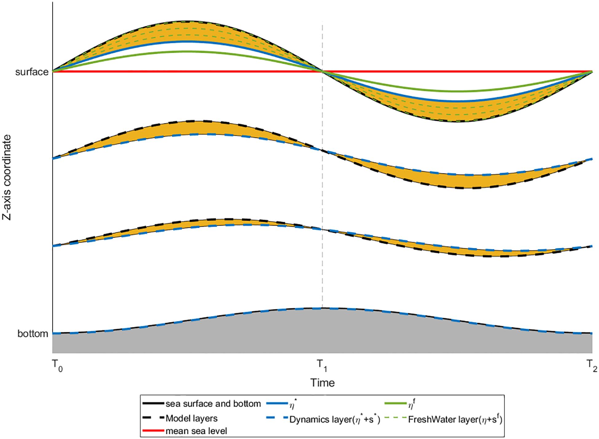
Figure 1. Diagram of the vertical stratification in ocean models with varying freshwater flux. The horizontal axis represents time and the vertical axis represents the vertical coordinates. The top black solid line indicates the sea surface, while the bottom black solid line represents the seabed. The blue solid line shows the variation in sea surface height caused by dynamic processes. The solid green line indicates the change in freshwater, where its elevation above mean sea level indicates that precipitation is greater than evaporation, otherwise it indicates that precipitation is less than evaporation. The black dashed line shows the original vertical stratification of the model. The blue dashed line indicates the vertical stratification formed solely by dynamic processes, excluding freshwater influences. The green dashed line represents the stratification based solely on freshwater changes. The yellow area illustrates the difference between the traditional stratification in the model and the actual dynamic processes, which is the artificial error.
In the Figure 1, from to , precipitation exceeds evaporation, leading to an increase in freshwater, and thus the actual dynamic process-induced sea surface fluctuations are lower than the traditional model stratification. Apart from the top layer, the yellow areas at the bottom should not represent freshwater with zero salinity but should be seawater. From to , precipitation is weaker than evaporation, resulting in a decrease in freshwater, so the sea surface fluctuations caused by the real dynamic processes are higher than the traditional stratification. The salt remaining after evaporation in the topmost yellow area should accumulate in the sub-surface layer. The salinity in the yellow areas of the remaining layers should not change. Therefore, we need to readjust the salinity distribution across different layers based on and to recalibrate the vertical salinity profile. Therefore, we propose a natural vertical distribution calculation scheme, as Equation 17, and then its vertical expansion yields Equations 18, 19.
where represents the weight coefficient. The proposed scheme does not alter the conservation relationship of salinity but changes the vertical distribution of salinity. The modified salinity is then reapplied to Equation 9.
To adjust the salinity distribution after re-stratification, the weight parameter needs to be calculated based on the real position. An indicator function can be given as Equation 20. It has been applied in Equation 21.
In order to simplify the formula for ease of writing and understanding, we have made the following simplifications, Equation 21. This simplification of Equation 21, makes the equation more concise and aesthetically pleasing, as well as easier to program.
where . Ultimately, we can derive a unified formula for the weight function.
Where , .
Because the decomposition in also leads to changes in other equations, it distinguishes itself from the virtual salt flux and natural boundary condition.
2.2 Boundary conditions
We treated the variation of freshwater in the surface layer as part of the ocean, encapsulated within . Referring to previous studies (Beron-Vera et al., 1999; Warren, 2009; Tseng et al., 2016; Verri et al., 2020), for the Boussinesq continuity and conservation equations of the salt, Equations 23 and 24, their boundary conditions at the surface layer are respectively Equations 25 and 26.
where, and respectively represents the horizontal and vertical diffusion term of salt. This implies that salt cannot undergo any form of advection or diffusion with the atmosphere through the air-sea interface.
For the virtual salt flux, its boundary conditions we specified in our experiment are satisfied by Equations 27 and 28.
where is a net addition of water to the ocean ().
For the natural boundary condition, its boundary conditions are satisfied by Equations 29 and 30.
The natural boundary condition preserves the vertical velocity in the surface, maintaining the driving effect of freshwater on seawater. The vertical diffusion term ensures the salinity balance of the water body. Our method has a similar form at . Substituting into Equation 27:
We do not consider the horizontal movement of freshwater in the surface layer, . Because of , the Equations 31 and 28 can be transformed to Equations 32 and 33.
Thus, the scheme we proposed can still preserve the driving process of freshwater on the ocean.
2.3 Application process
Our method is simpler and more user-friendly compared to approaches like VLR, with less changes to the original ocean model. These modifications are straightforward to implement using the equations provided in our manuscript. For instance, considering the POM, Figure 2 depicts the flow diagram of the POM. The modifications we introduced are highlighted in red boxes within this diagram. One modification pertains to the computation of surface elevation adjustments due to freshwater fluxes in the external mode. The other critical modification involves incorporating an NVCDS computational module after the calculations for convection and horizontal diffusion, but prior to vertical diffusion. This shows that our method does not require altering the original structure of the model.
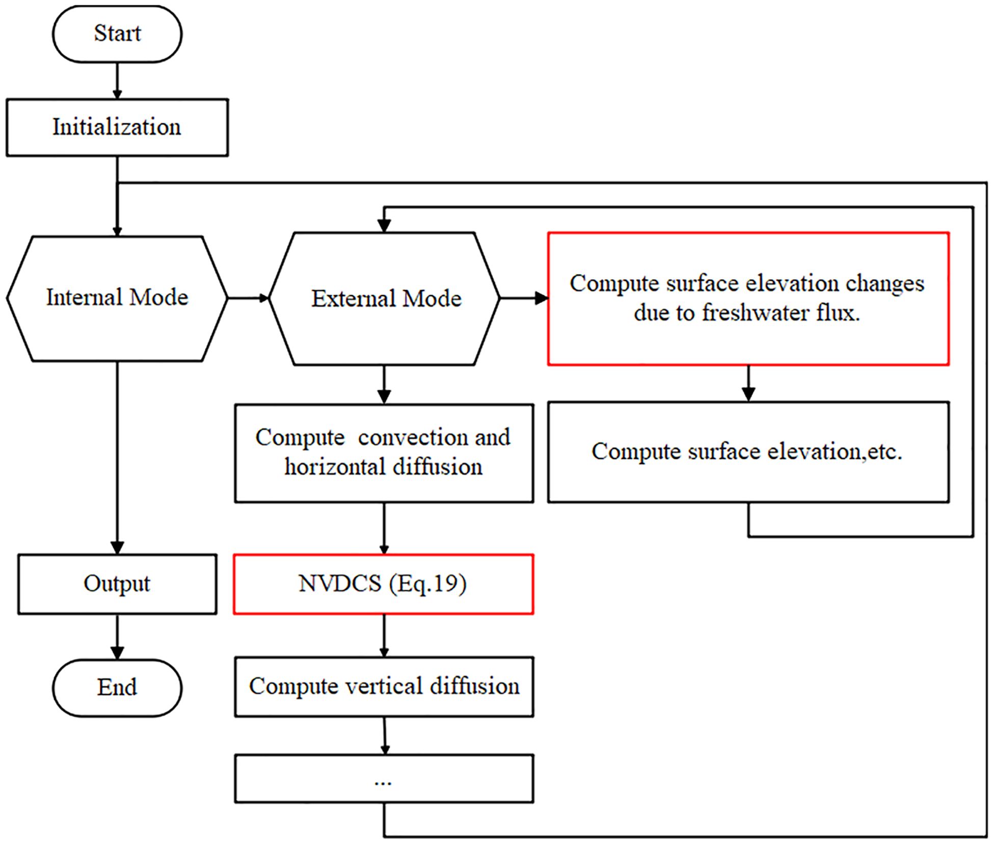
Figure 2. Flow diagram of the POM.
Figure 3 showcases the procedure flowchart for the NVDCS module. This module necessitates four input variables: the vertical distribution from both the preceding and current time steps, the increase in surface elevation due to freshwater fluxes, and the salinity values resulting from convection and horizontal diffusion computations. The first three variables are used to calculate weights according to Equation 22 in the manuscript, and then combined with the fourth input to compute the adjusted salinity using Equation 19. This adjusted salinity is subsequently employed in the ensuing step for vertical diffusion calculations. As illustrated, the computational sequence does not necessitate any additional reference frame conversions or interpolations, ensuring its modular integration. Furthermore, the parameters required as inputs are inherent to most existing ocean models, ensuring direct applicability.
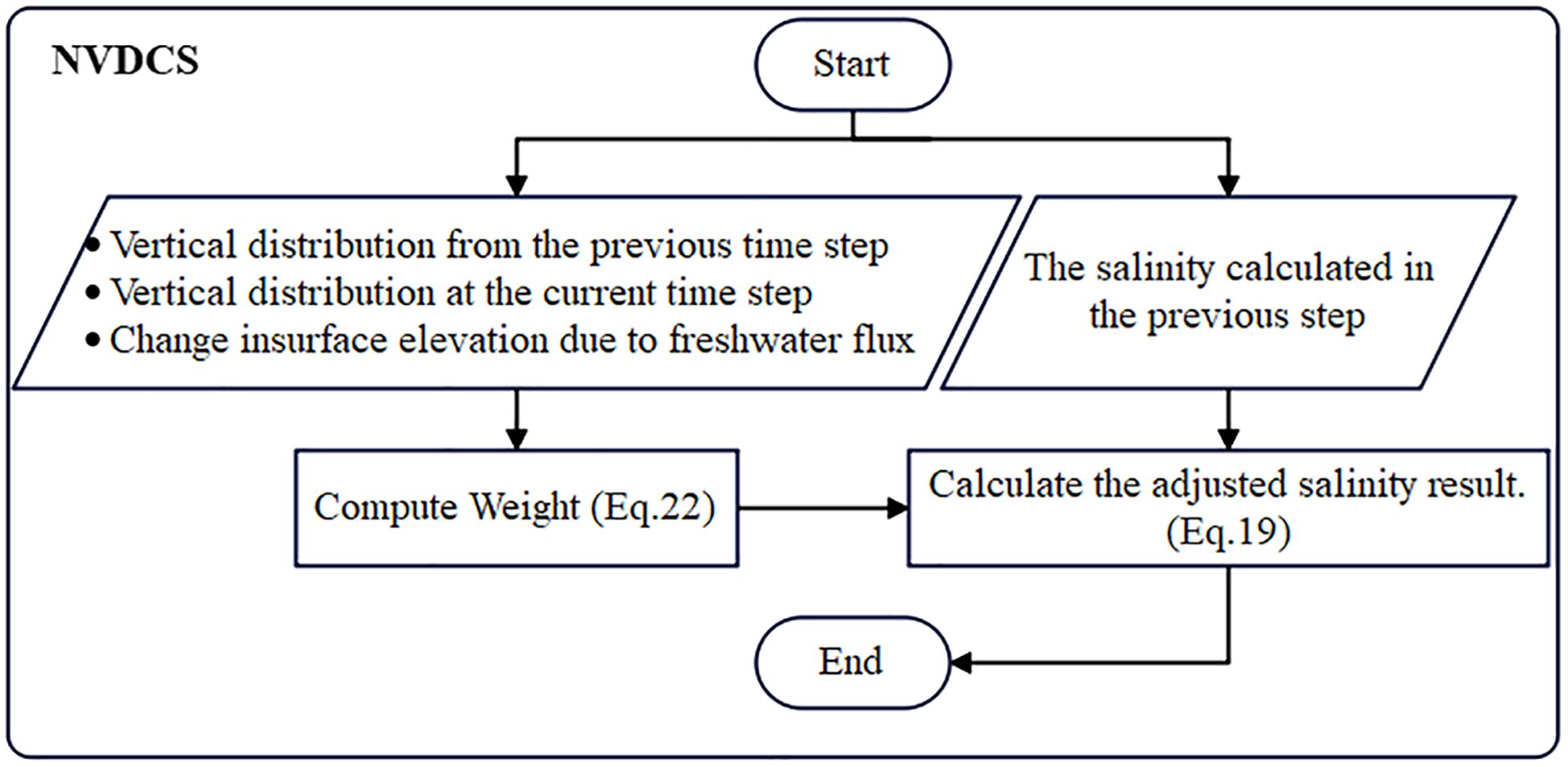
Figure 3. Flow diagram of NVDCS.
3 Sensitivity experiment
In order to verify that the calculation scheme can not only ensure the conservation of salinity, but also obtain a more reasonable vertical distribution like the use of virtual salt flux, three sensitivity experiments are set up. Select as the experimental area, with precipitation mainly at high latitudes and evaporation mainly at low latitudes. The horizontal resolution is , and the division is square grid, 29 layers vertically, the maximum water depth is 5700 meters. The time step of 1 hour, simulating 20 years. Horizontal viscosity coefficient and horizontal diffusion coefficient are and , respectively. Vertical viscosity coefficient and diffusion coefficient are . The initial temperature of the model is 12.5 and the initial salinity is 35 psu. There is no heat exchange in the sea surface forcing field and only freshwater fluxes are retained. The precipitation is (). In high latitudes, precipitation is the dominant factor while evaporation is the main contributor in low latitude, as depicted by the functional relationship shown in the left panel of Figure 4. Freshwater fluxes are affected by the latitude and ensure that the total water content is conserved throughout the simulation. The distribution of freshwater fluxes at the sea surface is illustrated in the right panel of Figure 4. The selection of these parameters and the function for freshwater distribution are referenced from Huang (1993).
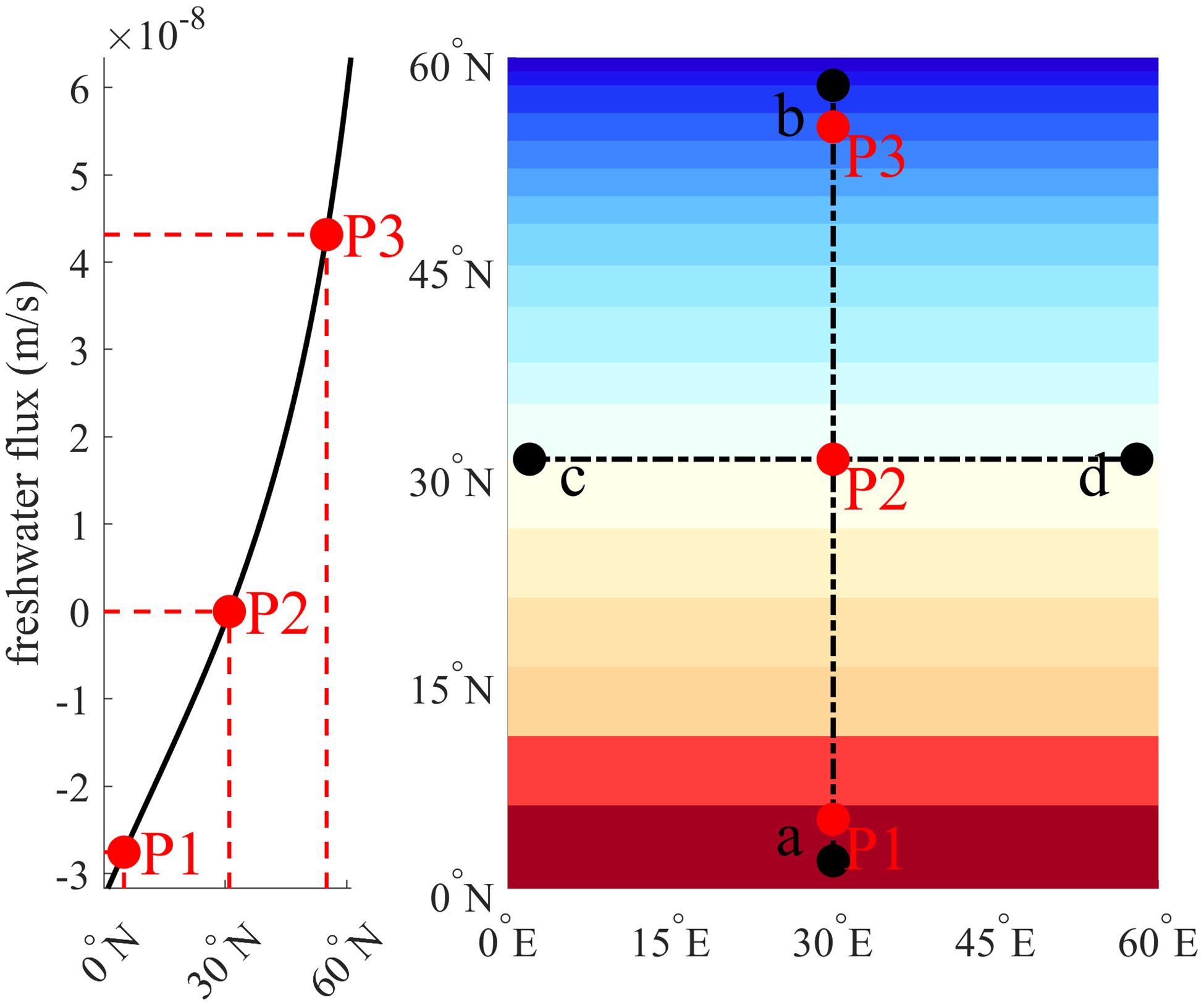
Figure 4. Left: Functional relationship between freshwater flux and latitude; Right: Horizontal distribution map of freshwater flux.
The control experiment settings are shown in Table 1. Experiment Ctrl and NoFlux use the original salinity calculation format of POM. The first column represents the experiment number, the second and third columns represent the boundary conditions at the sea surface, and the fourth column indicates whether our scheme was used to adjust the vertical distribution.
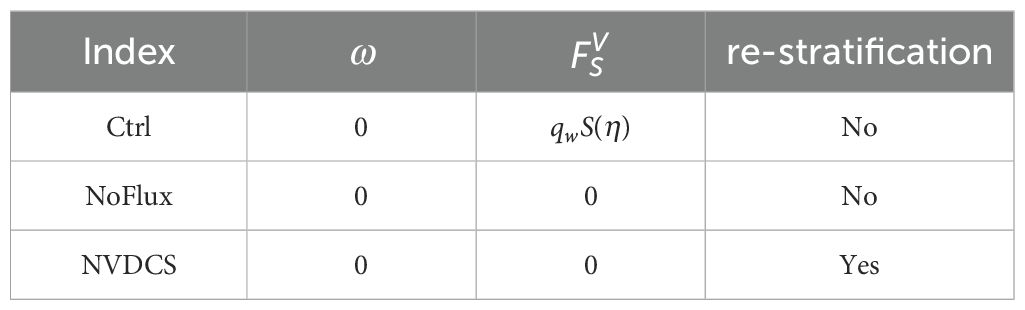
Table 1. The sensitivity experiments settings.
3.1 Comparison of conservation
The results presented in Figure 5 show the temporal evolution of the average salinity under different experimental conditions. It is evident that, in Ctrl experiment without implementing no salinity conservation mechanism, the salinity increases continuously over time, in sharp contrast to the other two experiments. This salinity imbalance has the potential to affect the model simulation in the long term. In contrast, the NoFlux and NVDCS experiments, which respectively do not use any salinity fluxes and use the NVDCS format to conserve salinity, show a remarkable stability of the average salinity over time. The maximum difference in the average salinity for the Ctrl experiment is 0.0017062 , while the maximum difference for the other two experiments is only , indicating that these conservation mechanisms have a significant impact on the model simulation.
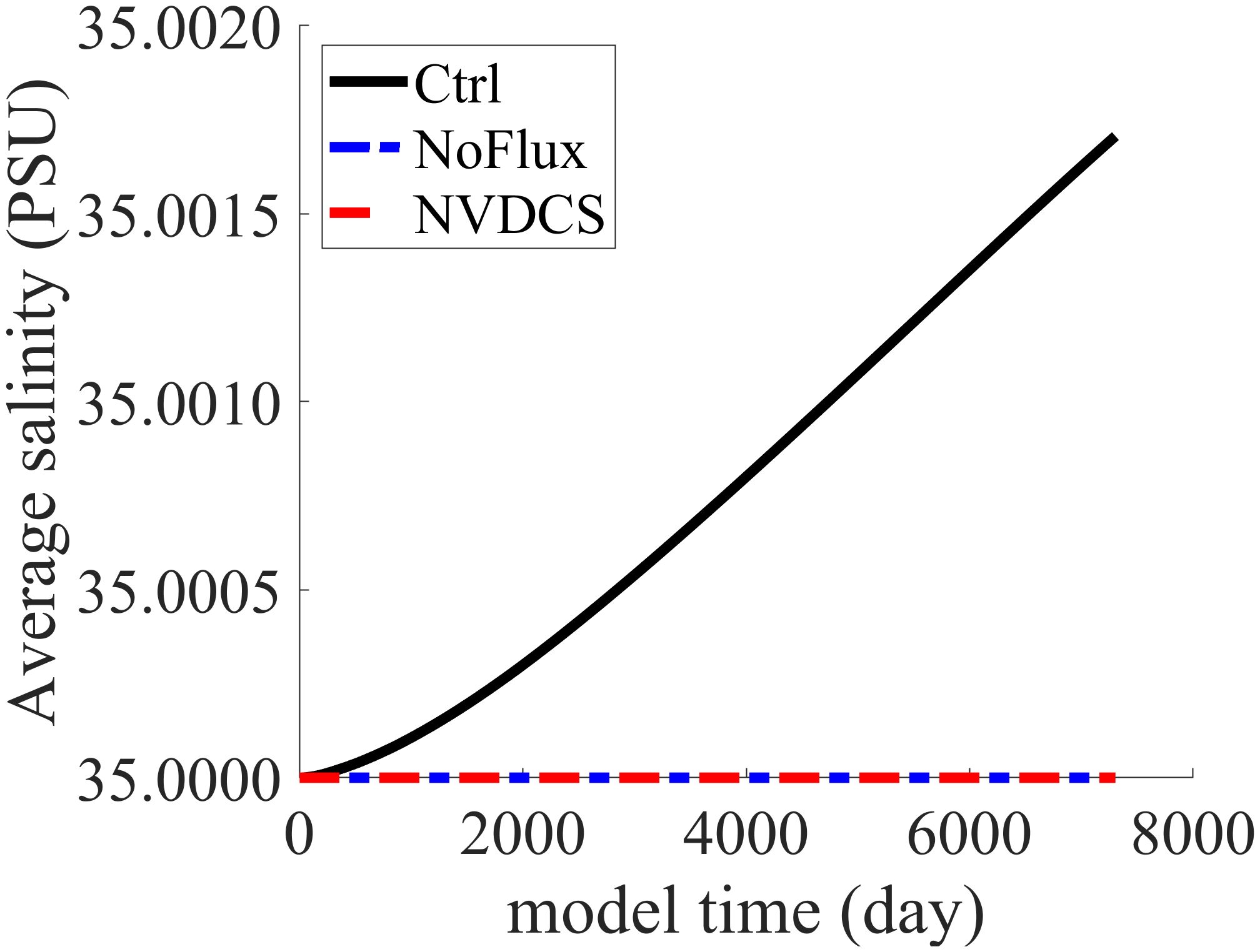
Figure 5. Comparison of average salinity in three experiments.
3.2 Comparison of the vertical distribution of salinity
The experimental area includes three points: P1 (5°N, 30°E), P2 (31°N, 30°E), and P3 (55°N, 30°E), as well as two cross sections, ab and cd, which span the longitude and latitude of the simulated area. The location of these points is illustrated in the right panel of Figure 4 and their locations on the horizontal precipitation distribution map are shown in the same figure. These three points represent regions of high evaporation, regions where evaporation and precipitation are balanced, and regions of high precipitation, respectively. Figures 6–8 show the vertical salinity changes at these three points over time. It is clear that both experimental Ctrl and NVDCS have similar processes of salinity propagation, but experimental NoFlux completely loses this process. In the panels b of those figures, the early stages of precipitation are sufficiently mixed with the bottom seawater, so that it has no stratification at all in the vertical direction. Obviously, the experimental NoFlux does not use salt flux, and the salinity caused by precipitation directly affected the deep sea. In the experiment, NVDCS simulates the vertical distribution of salinity well, and obtains a salinity distribution similar to that of the virtual salt flux Ctrl.
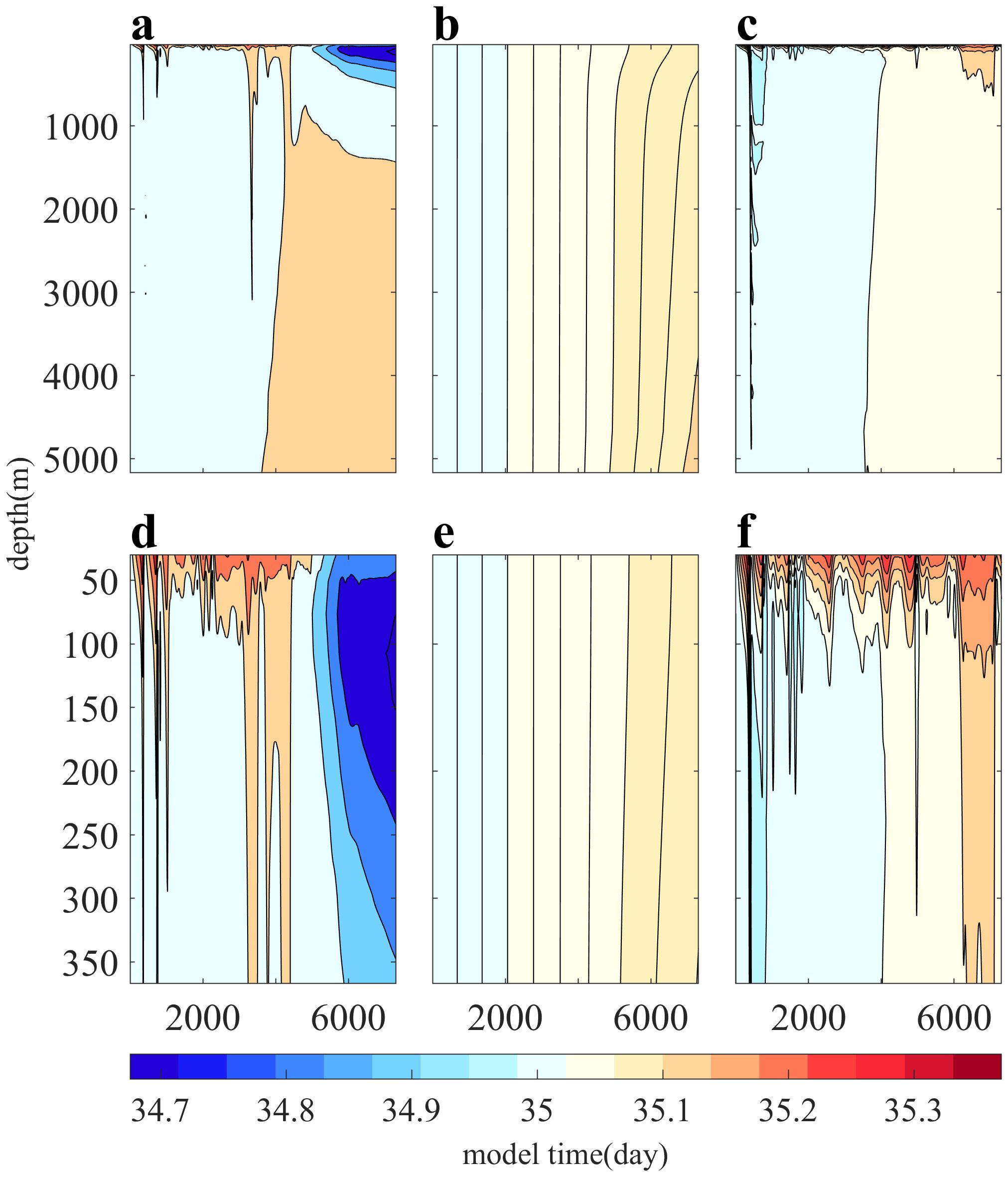
Figure 6. Time cross-section of vertical salinity distribution at point P1. The ordinate represents depth, the abscissa represents time during the simulation, and the color represents salinity. Panels (A, D) show the results of the control experiment. Panels (B, E) show the results of the experiment with no flux. Panels (C, F) show the calculation results of the experiment using the NVDCS. Panels (D–F) correspond to the salinity distribution of the upper surface layer in Panels (A–C), respectively.
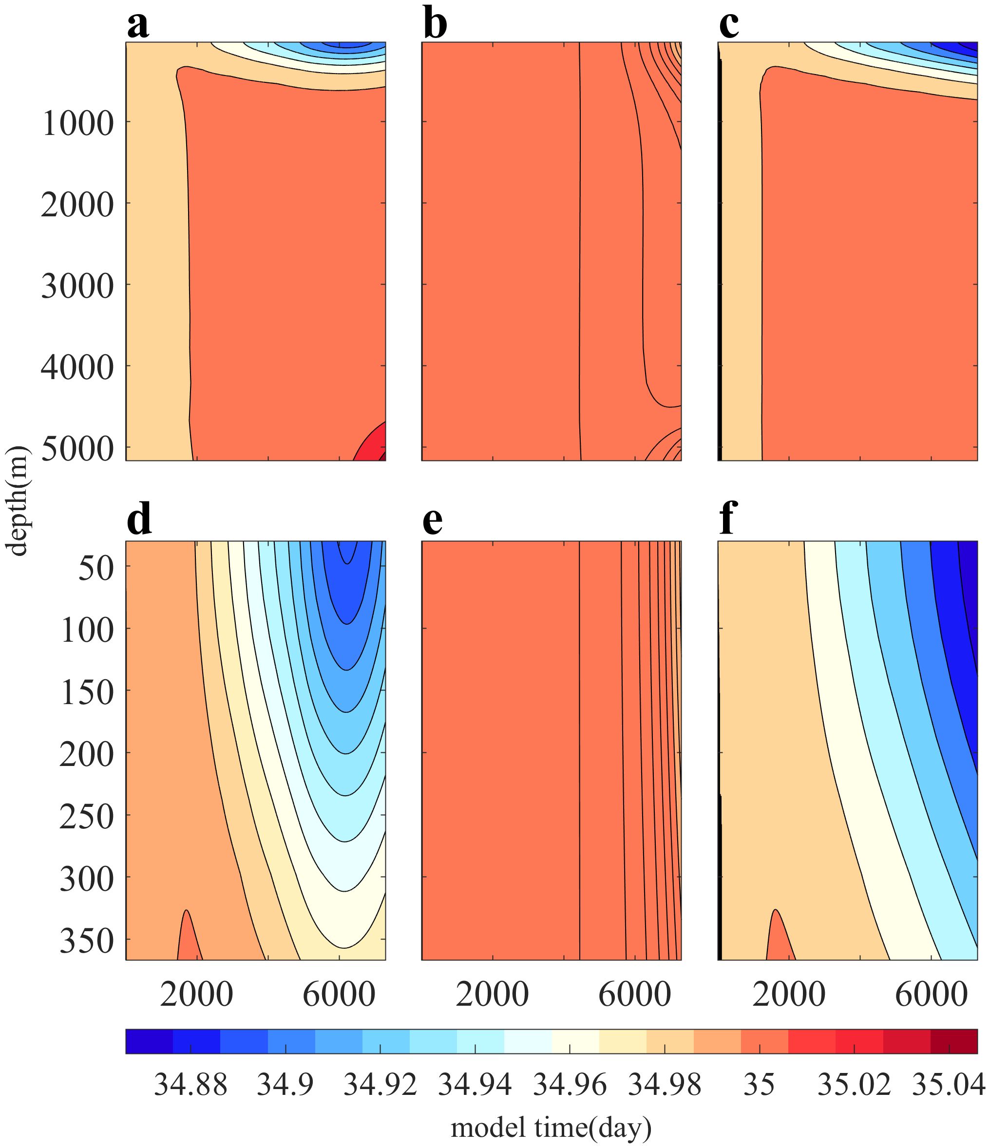
Figure 7. Time cross-section of vertical salinity distribution at point P2. The ordinate represents depth, the abscissa represents time during the simulation, and the color represents salinity. Panels (A, D) show the results of the control experiment, while Panels (B, E) show the results of the experiment with no flux. Panels (C, F) show the calculation results of the experiment using the NVDCS. Panels (D–F) correspond to the salinity distribution of the upper surface layer in Panels (A–C), respectively.
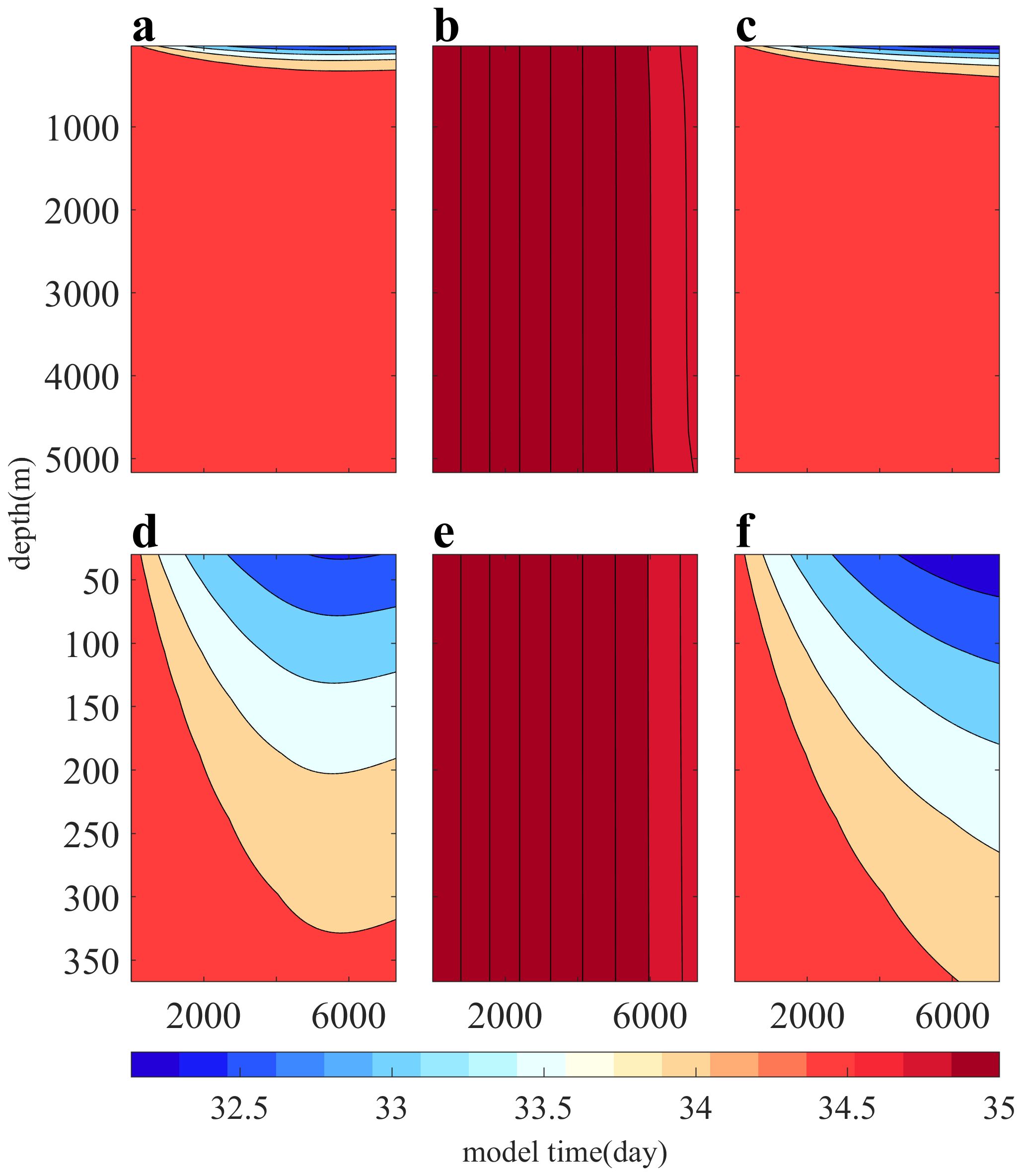
Figure 8. Time cross-section of vertical salinity distribution at point P3. The ordinate represents depth, the abscissa represents time during the simulation, and the color represents salinity. Panels (A, D) show the results of the control experiment, while Panels (B, E) show the results of the experiment with no flux. Panels (C, F) show the calculation results of the experiment using the NVDCS. Panels (D–F) correspond to the salinity distribution of the upper surface layer in Panels (A–C), respectively.
In the NoFlux experiment, salinity changes are mainly caused by the volume change of seawater as there is no salt flux. This volume change of seawater has a direct effect on the deep sea due to coordinate stratification. As a result, there is no mixing process in the middle, and no vertical distribution occurs (Figures 6B, E). In the Ctrl experiment, the salinity change is caused by two factors, the change in seawater volume, and the input and output effects of salt. The former has a smaller effect, while the latter is the main contributor. Therefore, there will be significant vertical distribution (Figures 6A, D). However, the change in seawater volume can also result in lower salinity of deep seawater in freshwater regions during the early stages of model operation, and higher salinity of deep seawater in high evaporation regions. As the model continues to operate, and salinity continues to increase, ultimately, both precipitation and evaporation regions will generally have higher salinity in the deep sea.
In the vicinity of Point P1, evaporation is the dominant process with a higher rate than precipitation, resulting in a decrease of freshwater at the sea surface. Figure 6 depicts the distribution of salinity under different numerical experiments. Experiment Ctrl and NVDCS demonstrate a clear formation of high salinity regions at the sea surface, without significant impact on the salinity of the deep seawater. However, Experiment NoFlux does not exhibit any stratification in the vertical direction, indicating that the salinity of different layers changes simultaneously with time, with no contribution from salinity convection and diffusion to the bottom layer. A comparison between Figures 6D and F reveals similar vertical distribution characteristics, demonstrating the clear effect of salinity transport from the surface to the bottom layer with time. In Figure 6, when evaporation is strong, the salinity of the upper surface in panel d is lower than that of panel f, resulting in greater salinity in the deep seawater of the former. This is due to the double effect mentioned earlier, where the strengthening of experimental Ctrl salinity is influenced not only by the sea surface salt flux but also by changes in unit volume after seawater stratification. As a result, the salinity of the deep seawater is enhanced to a certain extent. This effect is also responsible for the results of the NoFlux experiment. However, it is evident that the latter’s impact is smaller than that of the former, and experimental Ctrl can mask the influence of the latter by salt flux to produce an appropriate salinity stratification effect. In contrast, experimental NVDCS only relies on the natural convection and diffusion of salinity for its salinity distribution and transport into the deep sea.
Figures 6A and D clearly show the appearance of a low-salinity stream on the upper surface after 5000 days of simulation in experiment Ctrl. In Figure 9, it is also evident that the salinity gradient between the high and low latitudes of the sea surface in experiment Ctrl is smaller compared to that in the NVDCS experiment, and the western strengthening effect is more pronounced. As a result, a light saltwater flow moves south from the western boundary, reaching the southern boundary and spreading eastward. Although this phenomenon also exists in NVDCS, its larger salinity gradient makes the uniform western boundary reinforcement effect less effective north of 30°.
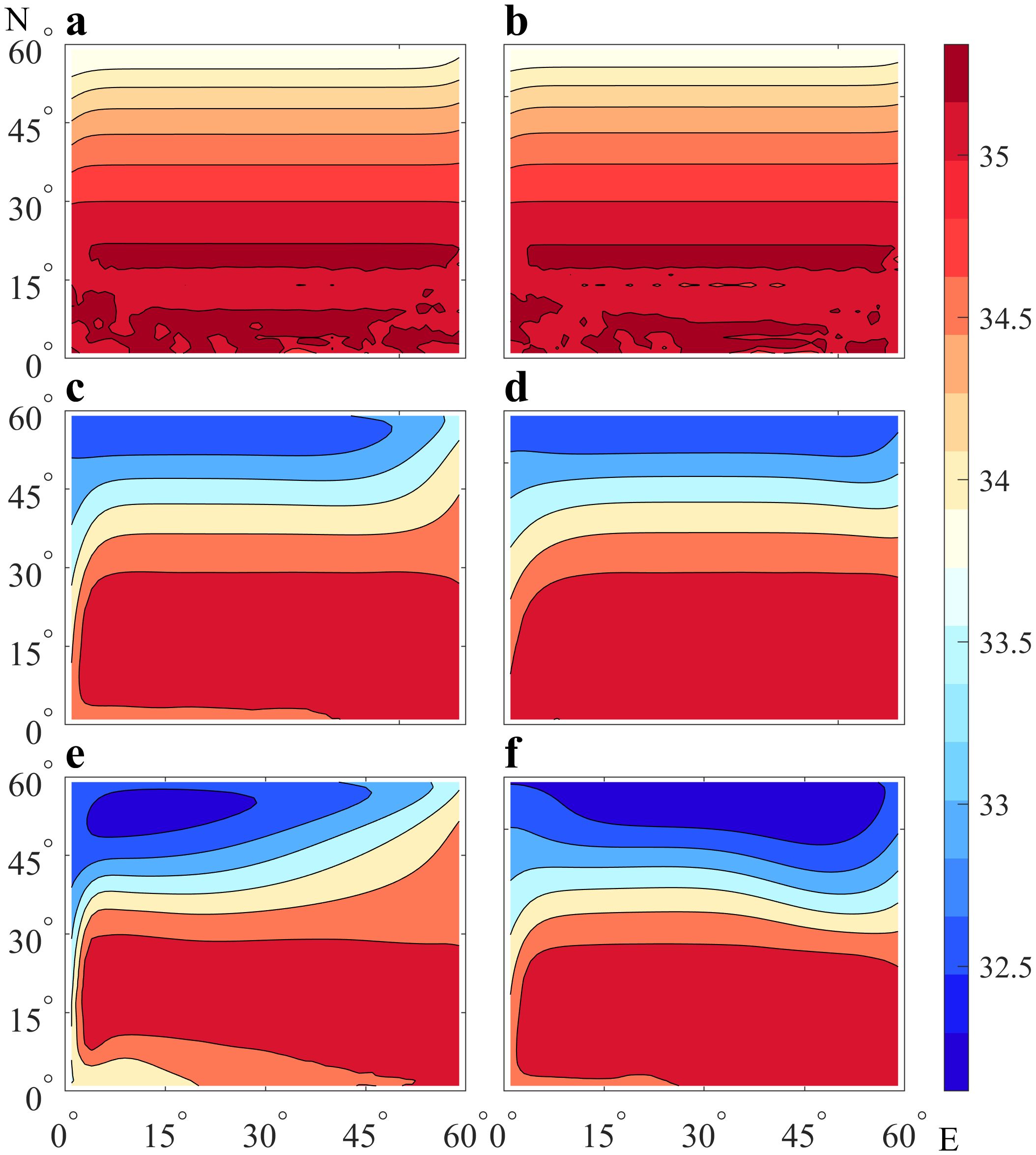
Figure 9. The horizontal distribution of surface salinity for different years in experiments Ctrl and NVDCS. Panels (A, C, E) respectively represent the results of experiment Ctrl after 1, 10, and 20 years of calculation. Panels (B, D, F) respectively represent the results after 1, 10, and 20 years of running experiment NVDCS.
At point P2, precipitation and evaporation are balanced, and the vertical distribution at this point is primarily influenced by the exchange with neighboring water bodies. Similar to Figure 6, Figures 7B and E exhibit no significant stratification. Although experiment Ctrl and NVDCS exhibit comparable structures, a comparison between Figures 7A and B reveals an increase in salinity at the bottom and a decrease in salinity at the sea surface for point P2 in the simulation. The effect is more pronounced in the NVDCS experiment. This is attributed to the transport of low brine from the sea surface in high latitudes towards the south and the northward transport of high brine from the deep layer in low latitudes. The NVDCS model can better simulate this phenomenon compared to other formats.
Point P3 is situated in a high latitude region with intense precipitation. Similar to Figures 6, 8B, E, 9 do not exhibit any stratification. However, Figures 8D and F clearly demonstrate the vertical salinity stratification state after the addition of fresh water, with Figure 8F indicating lower sea surface salinity compared to Figure 8D. Notably, Figure 8 does not reflect our previous theory, which suggests that experimental Ctrl, located in high latitudes, should have lower deep-sea salinity than experimental NVDCS. The horizontal distribution of seabed salinity after 1, 10, and 20 years of experimental Ctrl and NVDCS operation is depicted in Figure 10. This figure clearly illustrates that the seafloor salinity is higher in the high evaporation area, while it is lighter in the high precipitation area.
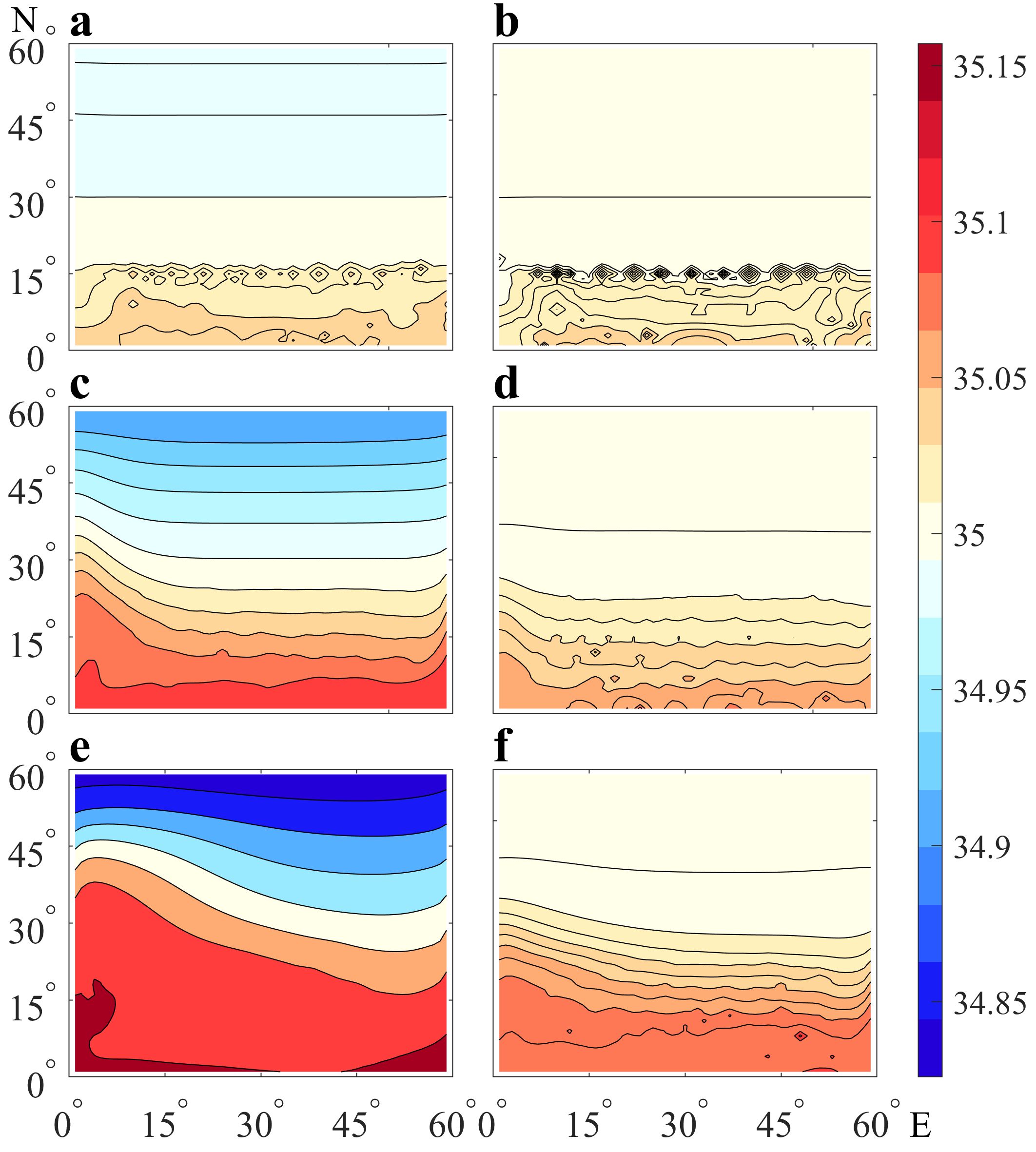
Figure 10. The horizontal distribution of seafloor salinity for different years in experiments Ctrl and NVDCS. Panels (A, C, E) respectively represent the results of experiment Ctrl after 1, 10, and 20 years of calculation. Panels (B, D, F) respectively represent the results after 1, 10, and 20 years of running experiment NVDCS.
When comparing Figures 9 and 10, it is observed that both the sea surface and seafloor of Experiment Ctrl had a stronger westward reinforcement compared to Experiment NVDCS. At the surface, Experiment NVDCS had a greater density difference which partly counteracted the north-to-south flow. At the seafloor, Experiment Ctrl responded rapidly to changes in sea surface salinity due to the dual effect of vertical stratification, leading to a greater density difference on the seafloor, which in turn facilitated the flow from south to north. Therefore, Experiment Ctrl demonstrated a stronger westward strengthening effect than NVDCS, regardless of the sea surface or seafloor.
The cross-sectional analysis of Figure 11 shows that both experiments exhibit similar salinity distribution and evolution over time. Freshwater is enriched in high latitudes and subsequently moves southward, leading to a gradual decrease in surface salinity. On the other hand, high saline water is enriched in low latitudes and moves northward via deep transport, leading to an increase in deep seawater salinity and expanding it towards the north. The pressure gradient forces influence the seawater flow, causing low-salt water to move southward. Due to the westward strengthening effect, the flow velocity on the west side increases, eventually leading to the formation of a stream of low-salt water on the southern surface. This observation provides evidence that NVDCS can effectively simulate the vertical salinity distribution without compromising its dynamic process, all while maintaining salinity conservation.
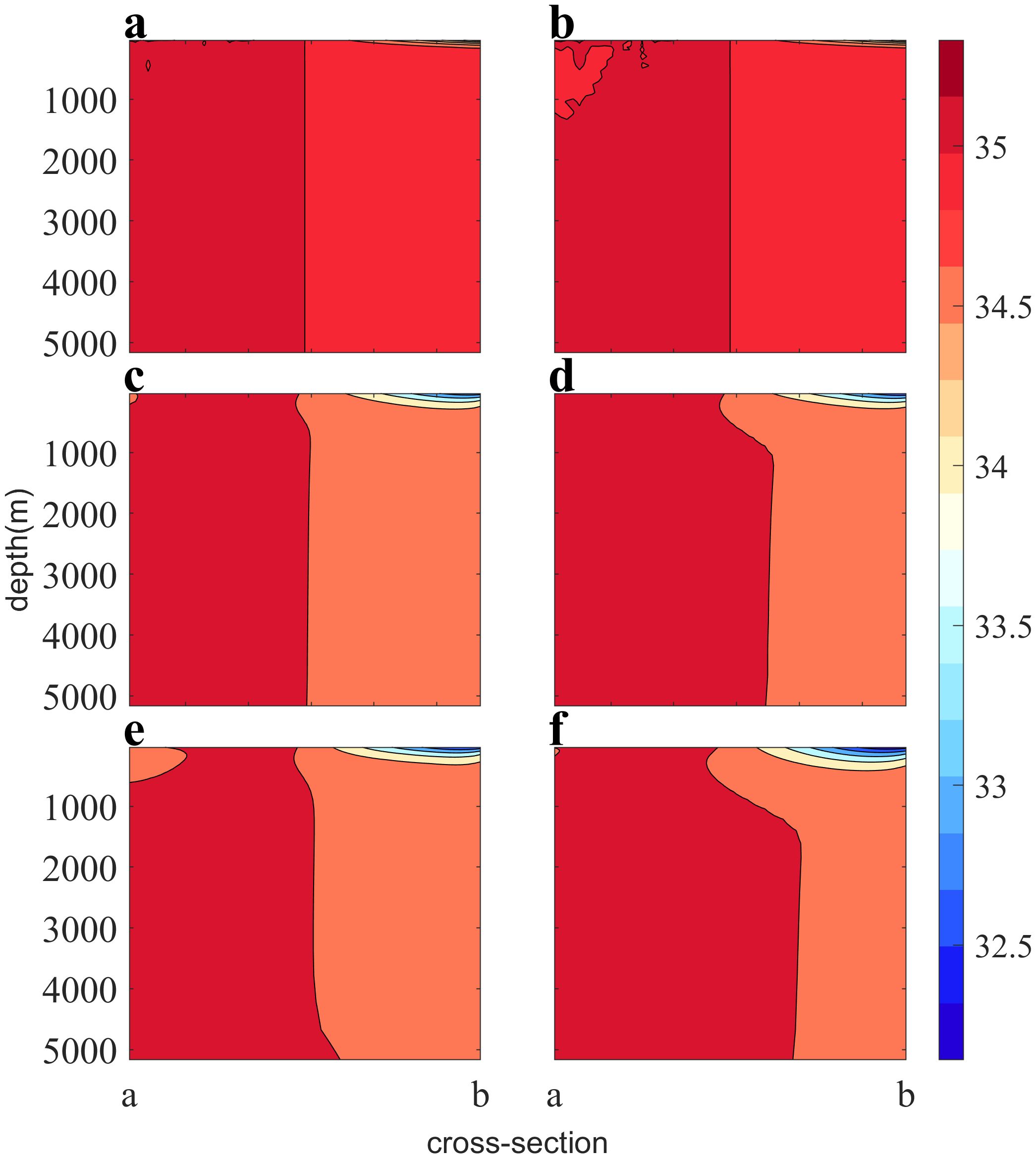
Figure 11. The vertical salinity distribution of section ab. The left panels (A, C, E) respectively display the results of experimental Ctrl after 1, 10, and 20 years of calculation, while the right panels (B, D, F) show the respectively results of experimental NVDCS after 1, 10, and 20 years of calculation.
To visually illustrate the differences between the two experiments, we have plotted the disparity of the results from the two experiments in Figure 12. Positive (negative) values indicate that the salinity in the Ctrl experiment is higher (lower) than in the NVDCS experiment. It is evident that, at the sea surface, the salinity in the Ctrl experiment is higher (lower) in regions of intense precipitation (evaporation) compared to our computational scheme. The opposite trend is observed at the seafloor. This once again confirms the presence of the aforementioned artificial error and demonstrates that our computational scheme effectively addresses this issue.
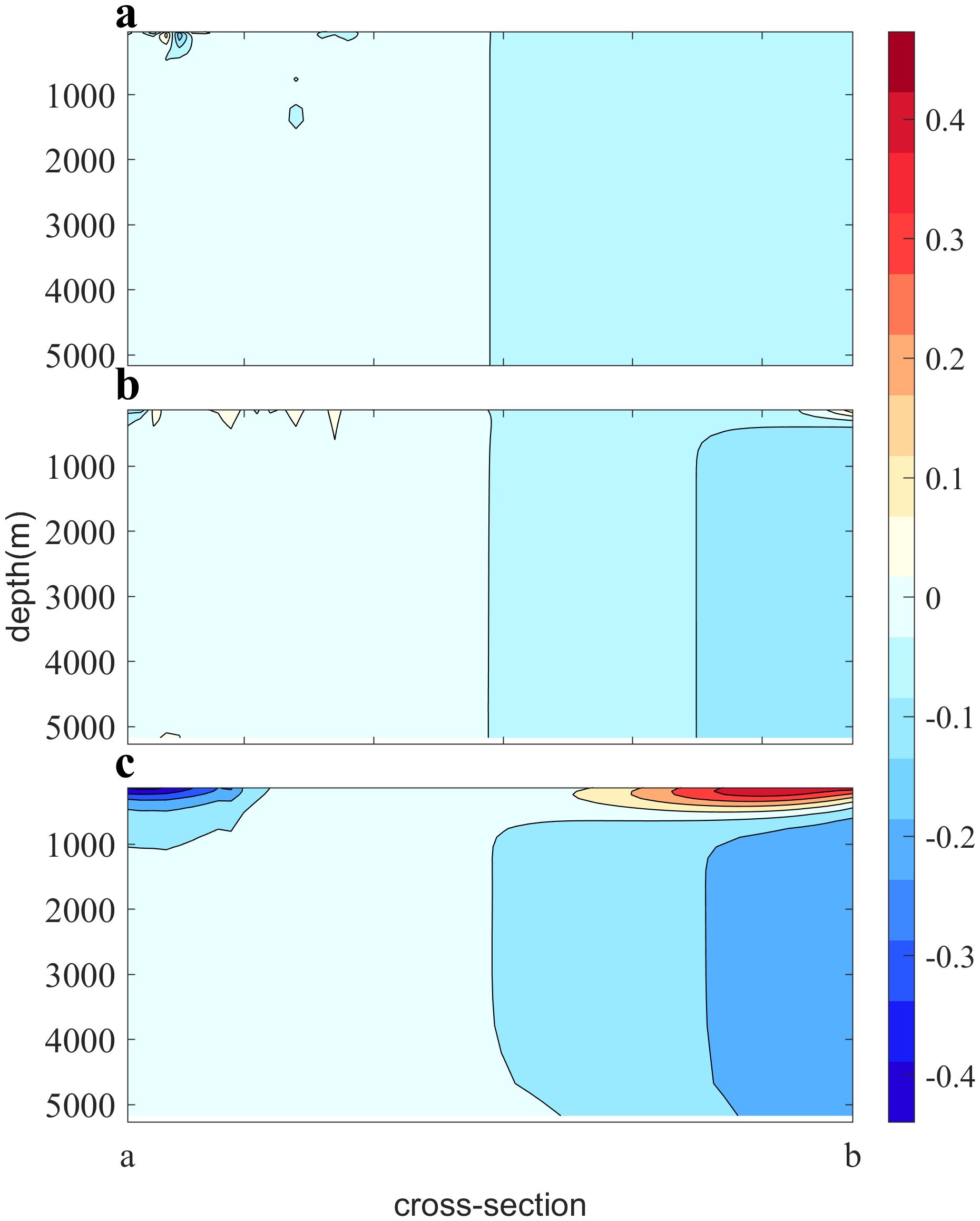
Figure 12. The difference in salinity between the experiments Ctrl and NVDCS at section ab. The panels (A–C) respectively display the results after 1, 10, and 20 years of calculation.
In the Figure 13, it can also be seen in the cross-sectional cd that both the Ctrl and NVDCS experiments have a similar structure, in which low-salinity water is concentrated on the east and west sides of the surface layer. The low-salinity water on the western side has a deeper depth, narrower cross-section, and a larger salinity gradient, especially in the Ctrl experiment, which further supports the westward strengthening effect observed in the experiment.
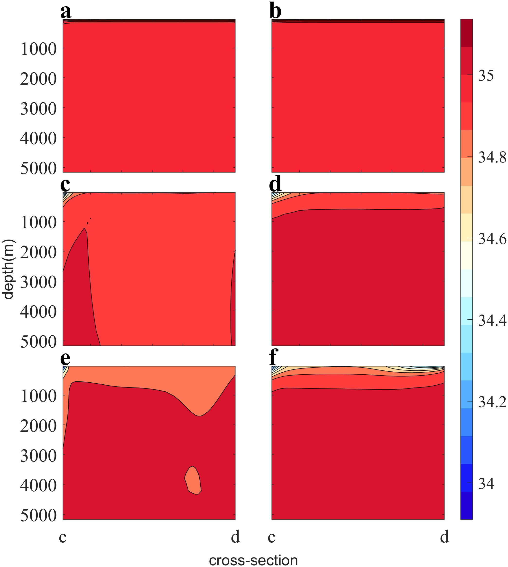
Figure 13. The vertical salinity distribution of section cd. The left panels (A, C, E) respectively display the results of experimental Ctrl after 1, 10, and 20 years of calculation, while the right panels (B, D, F) show the respectively results of experimental NVDCS after 1, 10, and 20 years of calculation.
3.3 Comparison of available potential energy
The introduction of freshwater flux, such as precipitation, will alter the mass and salinity of the ocean surface layer, as well as the pressure at the surface and throughout the deep water, thereby affecting the available potential energy. The original calculation method leads to the instantaneous transmission of salinity changes to the seafloor. Meanwhile, the “double effect” results in a greater density difference in the deep water, leading to an overall overestimation of available potential energy, as illustrated in Figure 14. Equation 34 represents the formula for calculating available potential energy proposed by Benoit and Beckers (2011).
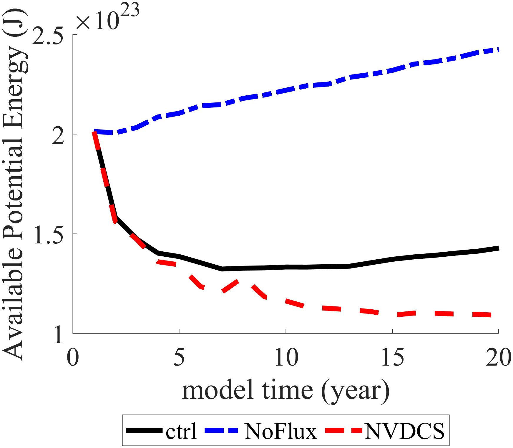
Figure 14. The comparison of available potential energy between three experiments.
4 Conclusions
In the free surface model, quasi-stationary coordinates adjust the vertical layers to encompass the entire water body within the computational domain in response to the undulation of seawater. The undulation is primarily caused by two factors. The first factor is the dynamic processes within the ocean, such as convergence and divergence of seawater. In ocean numerical model, this factor is caused by volume variations of every computational unit, resulting from changes in the net flow. Therefore, this factor exists throughout the entire water body. The adjustment of vertical layers aligns with fluid continuity and is natural and reasonable. The second factor is the volume change due to the inflow and outflow of surface freshwater. This should only affect the surface salinity. However, quasi-stationary coordinates, when adjusting vertical layers, do not differentiate between these two factors. Therefore, the changes at the sea surface layer affect the entire water body. Our proposed scheme aims to distinguish between these two factors. It preserves the original ocean dynamics while specially handling the influence of the surface freshwater. In external mode of the ocean model, we calculate the volume of freshwater entering and leaving the ocean. Throughout the model step process, we correct the salinity in each layer based on the calculated . The changes at the sea surface are separated, returning it to its natural state. Then the corrected salinity data is used in the salinity discretization formula to calculate for the next model time step.
In this study, we use the free surface POMgcs as an example to verity our proposed scheme. Our study domain is a closed experimental area of 60°×60°. From south to north, evaporation gradually weakens, and precipitation increases. We set up three experiments. The first experiment uses the commonly used virtual salt flux. The second experiment is the same as the first one but without virtual salt flux. And the last one uses our proposed NVDCS. Regarding salinity conservation, our proposed scheme maintains salt balance, similar to the second experiment. This indicates that, in our scheme, salt does not exchange with the external environment, and surface freshwater does not alter the total salt mass. Regarding the vertical distribution structure of salinity, the second experiment perfectly illustrates the previously mentioned artificial error. Salinity shows little vertical stratification. In the northern (southern) region with more precipitation (evaporation), the salinity in each vertical layer is lower (higher) than that in the southern (northern) region. The changes caused by the surface freshwater instantaneously affect the entire water body. After using virtual salt flux, the model artificially constructs the vertical stratification of salinity. However, in comparison to our scheme, where the sea surface salinity is lower (or higher), the salinity at the seafloor is also lower (or higher). This indicates that quasi-stationary coordinates still distribute changes at the sea surface throughout the entire water body. Our proposed scheme effectively addresses this artificial error.
One of the impacts of this artificial error is the overestimation of available potential energy. The original calculation method causes salinity changes to be instantaneously transmitted to the seafloor, increasing the density gradient centrifugation under the sea surface, resulting in an overall overestimation of available potential energy.
In addition to salinity, freshwater has physical properties such as temperature, velocity, momentum, and more. In the free surface model, those properties of sea surface will change with the inflow and outflow of surface freshwater. Quasi- stationary coordinates will instantaneously influence these changes throughout the entire water body. This artificial error does not only affect salinity. This instantaneous error could amplify inaccuracies in seawater energy and density. These accumulated deviations may alter the dynamic processes within the ocean, leading to artificial eddies. These potential eddies may introduce more difficult-to-estimate impacts. The calculation scheme proposed in this paper can be applied to all the aforementioned physical quantities. The various issues and challenges, as well as the practical application of this method, will be the focus of our upcoming research and exploration.
Now some researchers have noticed this problem and proposed solutions such as VLR. In the following research, we will also compare with other methods, verify the differences between different methods, and explore the differences.
Data availability statement
The datasets presented in this study can be found in online repositories. The names of the repository/repositories and accession number(s) can be found below: https://doi.org/10.6084/m9.figshare.22345117.
Author contributions
YL: Writing – original draft. GH: Writing – review & editing. WL: Writing – review & editing. XW: Writing – review & editing. LC: Writing – review & editing. GZ: Writing – review & editing.
Funding
The author(s) declare financial support was received for the research, authorship, and/or publication of this article. This work was supported in part by the National Key Research and Development Program under Grant 2023YFC3107800 and in part by the National Natural Science Foundation under Grant 42376190.
Conflict of interest
The authors declare that the research was conducted in the absence of any commercial or financial relationships that could be construed as a potential conflict of interest.
Publisher’s note
All claims expressed in this article are solely those of the authors and do not necessarily represent those of their affiliated organizations, or those of the publisher, the editors and the reviewers. Any product that may be evaluated in this article, or claim that may be made by its manufacturer, is not guaranteed or endorsed by the publisher.
References
Adcroft A., Campin J. (2004). Rescaled height coordinates for accurate representation of free-surface flows in ocean circulation models. Ocean Model. 7, 269–284. doi: 10.1016/j.ocemod.2003.09.003
Adcroft A., Anderson W., Balaji V., Blanton C., Bushuk M., Dufour C. O., et al. (2019). The GFDL global ocean and sea ice model OM4.0: model description and simulation features. J. Adv. Modeling Earth Syst. 11, 3167–3211. doi: 10.1029/2019MS001726
Adcroft A., Hallberg R. (2006). On methods for solving the oceanic equations of motion in generalized vertical coordinates. Ocean Model. 11, 224–233. doi: 10.1016/j.ocemod.2004.12.007
Babin S. M., Young G. S., Carton J. A. (1997). A new model of the oceanic evaporation duct. J. Appl. Meteorology Climatology 36, 193–204. doi: 10.1175/1520-0450(1997)036<0193:ANMOTO>2.0.CO;2
Barnier B., Siefridt L., Marchesiello P. (1995). Thermal forcing for a global ocean circulation model using a three-year climatology of ECMWF analyses. J Mar Syst. 6 (4), 363–380. doi: 10.1016/0924-7963(94)00034-9
Benoit C., Beckers J. (2011). Introduction to geophysical fluid dynamics: physical and numerical aspects. Second Edition. (MA USA: Academic press). doi: 10.1007/s00024-015-1091-0
Beron-Vera F. J., Ochoa J., Ripa P. (1999). A note on boundary conditions for salt and freshwater balances. Ocean Model. (Oxford) 1, 111–118. doi: 10.1016/S1463-5003(00)00003-2
Bleck R. (2002). An oceanic general circulation model framed in hybrid isopycnic-Cartesian coordinates. Ocean Model. (Oxford) 4, 55–88. doi: 10.1016/S1463-5003(01)00012-9
Boutin J., Chao Y., Asher W. E., Delcroix T., Drucker R., Drushka K., et al. (2016). Satellite and in situ salinity: understanding near-surface stratification and subfootprint variability. Bull. Amer. Meteor. Soc. 97 (8), 1391–1407. doi: 10.1175/BAMS-D-15-00032.1
Bryan F. (1986). High-latitude salinity effects and interhemispheric thermohaline circulations. Nature 323, 301–304. doi: 10.1038/323301a0
Ezer T., Mellor G. (2004). A generalized coordinate ocean model and a comparison of the bottom boundary layer dynamics in terrain-following and in z-level grids. Ocean Model. 6, 379–403. doi: 10.1016/S1463-5003(03)00026-X
Filimonova M., Trubetskova M. (2005). “Calculation of evaporation from the Caspian Sea surface,” in Proceedings of the International Symposium on Stochastic Hydraulics, Nijmegen, The Netherlands, pp. 63–65.
Furue R., Takatama K., Sasaki H., Schneider N., Nonaka M., Taguchi B. (2018). Impacts of sea-surface salinity in an eddy-resolving semi-global OGCM. Ocean Model. 122, 36–56. doi: 10.1016/j.ocemod.2017.11.004
Garcia-Soto C., Cheng L., Caesar L., Schmidtko S., Jewett E. B., Cheripka A., et al. (2021). An overview of ocean climate change indicators: sea surface temperature, ocean heat content, ocean pH, dissolved oxygen concentration, arctic sea ice extent, thickness and volume, sea level and strength of the AMOC (Atlantic meridional overturning circulation). Front. Mar. Sci. 8. doi: 10.3389/fmars.2021.642372
Griffies S. M., Adcroft A., Hallberg R. W. (2020). A primer on the vertical Lagrangian-remap method in ocean models based on finite volume generalized vertical coordinates. J. Adv. Modeling Earth Syst. 12, e2019MS001954. doi: 10.1029/2019MS001954
Haney R. L. (1971). Surface thermal boundary condition for ocean circulation models. J. Phys. Oceanography 1, 241–248. doi: 10.1175/1520-0485(1971)001<0241:STBCFO>2.0.CO;2
Hedstrom K. S. (2018). Technical manual for a coupled sea-ice/ocean circulation model (version 5) (Alaska OCS Region: US Dept. of the Interior, Bureau of Ocean Energy Management), 182 pp. OCS Study BOEM 2018-007.
Huang R. X. (1993). Real freshwater flux as a natural boundary condition for the salinity balance and thermohaline circulation forced by evaporation and precipitation. J. Phys. Oceanography 23, 2428–2446. doi: 10.1175/1520-0485(1993)023<2428:RFFAAN>2.0.CO;2
Huang R. X., Schmitt R. W. (1993). The Goldsbrough-Stommel circulation of the world oceans. J. Phys. Oceanography 23, 1277–1284. doi: 10.1175/1520-0485(1993)023<1277:TGCOTW>2.0.CO;2
Killworth P. D., Smeed D. A., Nurser A. J. G. (2000). The effects on ocean models of relaxation toward observations at the surface. J. Phys. Oceanography 30, 160–174. doi: 10.1175/1520-0485(2000)030<0160:TEOOMO>2.0.CO;2
Liu Y., Cheng L., Pan Y., Abraham J., Zhang B., Zhu J., et al. (2022a). Climatological seasonal variation of the upper ocean salinity. Int. J. Climatology 42, 3477–3498. doi: 10.1002/joc.7428
Liu Y., Cheng L., Pan Y., Tan Z., Abraham J., Zhang B., et al. (2022b). How well do CMIP6 and CMIP5 models simulate the climatological seasonal variations in ocean salinity? Adv. atmospheric Sci. 39, 1650–1672. doi: 10.1007/s00376-022-1381-2
Lorenz M., Klingbeil K., Burchard H. (2021). Impact of evaporation and precipitation on estuarine mixing. J. Phys. Oceanography 51, 1319–1333. doi: 10.1175/JPO-D-20-0158.1
Mellor G. L., Häkkinen S. M., Ezer T., Patchen R. C. (2002). “A generalization of a sigma coordinate ocean model and an intercomparison of model vertical grids,” in Pinardi N., Woods J. D. eds. Ocean Forecasting: Conceptual Basis and Applications. (New York: Springer), 55–72. doi: 10.1007/978-3-662-22648-3_4
Nurser A. J. G., Griffies S. M. (2019). Relating the diffusive salt flux just below the ocean surface to boundary freshwater and salt fluxes. J. Phys. Oceanography 49, 2365–2376. doi: 10.1175/JPO-D-19-0037.1
Oka A., Hasumi H. (2004). Effects of freshwater forcing on the Atlantic deep circulation: a study with an OGCM forced by two different surface freshwater flux datasets. J. Climate 17, 2180–2194. doi: 10.1175/1520-0442(2004)017<2180:EOFFOT>2.0.CO;2
Prange M., Gerdes R. (2006). The role of surface freshwater flux boundary conditions in Arctic Ocean modelling. Ocean Model. 13, 25–43. doi: 10.1016/j.ocemod.2005.09.003
Rao R. R. (2003). Seasonal variability of sea surface salinity and salt budget of the mixed layer of the north Indian Ocean. J. Geophysical Res. 108, 1–9. doi: 10.1029/2001JC000907
Rooth C. (1982). Hydrology and ocean circulation. Prog. Oceanography 11, 131–149. doi: 10.1016/0079-6611(82)90006-4
Rosenblum E., Stroeve J., Gille S. T., Lique C., Fajber R., Tremblay L. B., et al. (2022). Freshwater input and vertical mixing in the Canada Basin’s seasonal halocline: 1975 versus 2006–12. J. Phys. Oceanography 52, 1383–1396. doi: 10.1175/JPO-D-21-0116.1
Roullet G., Madec G. (2000). Salt conservation, free surface, and varying levels: A new formulation for ocean general circulation models. J. Geophysical Research: Oceans 105, 23927–23942. doi: 10.1029/2000JC900089
Tseng Y., Bryan F. O., Whitney M. M. (2016). Impacts of the representation of riverine freshwater input in the community earth system model. Ocean Model. 105, 71–86. doi: 10.1016/j.ocemod.2016.08.002
Verri G., Pinardi N., Bryan F., Tseng Y., Coppini G., Clementi E. (2020). A box model to represent estuarine dynamics in mesoscale resolution ocean models. Ocean Model. 148, 101587. doi: 10.1016/j.ocemod.2020.101587
Vialard J., Delecluse P. (1998). An OGCM study for the TOGA decade. part I: Role of salinity in the physics of the Western Pacific fresh pool. J. Phys. Oceanography 28, 1071–1088. doi: 10.1175/1520-0485(1998)028<1071:AOSFTT>2.0.CO;2
Wallcraft A. J., Metzger E. J., Carroll S. N. (2009). Software design description for the HYbrid coordinate ocean model (HYCOM) version 2.2. Tech. Rep., Naval Research Laboratory, Stennis Space Center, MS. doi: 10.21236/ADA494779
Warren B. A. (2009). Note on the vertical velocity and diffusive salt flux induced by evaporation and precipitation. J. Phys. oceanography 39, 2680–2682. doi: 10.1175/2009JPO4069.1
Keywords: ocean model, freshwater flux, salinity conservation, vertical distribution, quasi-stationary coordinates
Citation: Li Y, Han G, Li W, Wu X, Cao L and Zhou G (2024) A natural vertical distribution calculation scheme for salinity simulation in free-surface model with quasi-stationary coordinates. Front. Mar. Sci. 11:1347088. doi: 10.3389/fmars.2024.1347088
Received: 30 November 2023; Accepted: 26 July 2024;
Published: 13 August 2024.
Edited by:
Benjamin Rabe, Alfred Wegener Institute Helmholtz Centre for Polar and Marine Research (AWI), GermanyReviewed by:
John Patrick Abraham, University of St. Thomas, United StatesYinglong Zhang, College of William & Mary, United States
Copyright © 2024 Li, Han, Li, Wu, Cao and Zhou. This is an open-access article distributed under the terms of the Creative Commons Attribution License (CC BY). The use, distribution or reproduction in other forums is permitted, provided the original author(s) and the copyright owner(s) are credited and that the original publication in this journal is cited, in accordance with accepted academic practice. No use, distribution or reproduction is permitted which does not comply with these terms.
*Correspondence: Wei Li, bGl3ZWkxOTc4QHRqdS5lZHUuY24=; Guijun Han, Z3VuanVuX2hhbkB0anUuZWR1LmNu