 Miaomiao Xu
 Yihe Wang
 Zhixuan Feng
 Hui Wu1,2,3,4
95% of researchers rate our articles as excellent or good
Learn more about the work of our research integrity team to safeguard the quality of each article we publish.
Find out more
ORIGINAL RESEARCH article
Front. Mar. Sci. , 09 February 2024
Sec. Coastal Ocean Processes
Volume 11 - 2024 | https://doi.org/10.3389/fmars.2024.1345940
Phytoplankton frequently blooms in estuaries and coastal seas. Numerous dynamic processes affect these regions, generating complex hydrodynamics that induce intense phytoplankton variability over multiple time scales. Especially, the variability over time scales of 100-101 days (event-scale) is a strong signal that is fundamental to coastal aquatic environments and ecosystems. Based on the historical monitoring of harmful algal bloom events and a fully coupled hydrodynamics-sediment-ecosystem numerical model, this study explored horizontal distribution patterns of the phytoplankton maximum off the Changjiang River Estuary over multiple time scales. Our results showed that the bloom events typically lasted less than a week and horizontal distribution of the horizontal chlorophyll maximum varied over the time scale of days. Tidal forcing was shown to dominate the periodic phytoplankton variability. The variations of river runoff and wind forcing also modulated this variability and added more disturbances. Increased runoff and enhanced summer monsoon wind caused the horizontal chlorophyll maximum to physically extend further offshore, while they also biologically stimulated phytoplankton blooms. The analysis of the time scale showed that the regulation of horizontal chlorophyll maximum responds faster to physical effects than in biological ones. At the same time, during neap tides, the adjustment of phytoplankton to the disturbances associated with the hydrodynamic processes was stably salient. Such adjustment was based on the adaptation to light availability and nutrient supply. This study contributes to the understanding of phytoplankton variability in estuaries affected by multiple physical-biological processes over the time scale of days and benefits to the management of environmental conservation.
Estuarine and coastal regions, which are among the most productive aquatic ecosystems (Pauly and Christensen, 1995; Agardy et al., 2005), are characterized by various environmental conditions and diverse marine biota (Lohrenz et al., 1990; Loreau et al., 2001; Cullen et al., 2002) due to the terrestrial load produced by natural variations and human activities (Rabalais et al., 1996; Barbier et al., 2011). On one hand, the high natural productivity of these regions benefits human lives, nursing fishery grounds, and marine agriculture activities (Grimes, 2001). On the other hand, excess primary productivity threatens aquatic environments, causing ecological problems such as harmful algal bloom events and hypoxia (Justi et al., 1996; Rabalais et al., 2001; Li et al., 2014). Phytoplankton variability, which is the primary driver of marine ecosystems and largely determines their health, is therefore of great importance in terms of the functions and services provided to human beings.
The patterns of phytoplankton variability are often examined both at the intra-annual and inter-annual time scales (Cloern and Jassby, 2010). In temperate oceans, the general pattern of intra-annual variability is represented by seasonal variations. In addition, variations over short time scales, such as spring-neap, daily, or hourly scales, are also part of this type of variability (Lucas, 2010; Wang et al., 2023). In estuarine and coastal waters, nutrient inputs generally stimulate phytoplankton variations over short time scales, which primarily manifest as the development and recession of algal blooms in various hotspots (Yin, 2003; Paerl et al., 2010). In some estuaries, eutrophication has been suggested as a causative factor of algal blooms (Moncheva et al., 2001; Heil et al., 2005). Exceptional phytoplankton variations and bloom events over short time scales are regarded as the response to dynamic fluctuations in high-nutrient habitats (Cloern and Jassby, 2010).
The complex estuarine hydrodynamics interacting with multiple physical processes determine biogeochemical responses at different time scales, which occur in estuarine regions and are a challenging topic for marine researchers. Numerous studies have focused on the patterns of phytoplankton variability and its potential mechanisms in estuaries worldwide, notably in Chesapeake Bay (Pease et al., 2021), Manila Bay (Siringan et al., 2008), the Pearl River Estuary (Shen et al., 2012), the Changjiang River Estuary (Zhou et al., 2017), and the Gulf of Mexico (Wynne et al., 2005), obtaining valuable insights. Estuaries are the areas where riverine and oceanic waters meet. The hydrodynamics in these regions inherently induce sharp variations in water properties and favor the concentration of phytoplankton, causing frequent bloom events on estuarine fronts (Franks, 1992). The position and structure of the riverine front and the distribution of the water components that affect phytoplankton growth (such as nutrients and suspended particulate matter) jointly determine the spatiotemporal distribution of phytoplankton (Cullen et al., 2002). The variation of key dynamic processes causes the alternation of the frontal structure and modifies environmental elements, eventually influencing phytoplankton distribution. Previous studies have suggested that changes in tide, wind, and runoff play a role in phytoplankton variability (Kimmerer et al., 2012; Llebot et al., 2011; Cadier et al., 2017; Jiang and Xia, 2017; Phlips et al., 2020). On one hand, these key processes alter the horizontal convergent status of the front and the vertical water stabilization, which directly influence the position of phytoplankton accumulation and residence time of phytoplankton transport (Odebrecht et al., 2015; Cloern et al., 2017; Sun et al., 2020); on the other hand, they regulate phytoplankton growth, for example by improving solar irradiation or supplying more nutrients (Bode et al., 2017; Cira et al., 2021). However, except for the inherent periodic tidal forcing, the timing and fluctuation of other dynamic processes, such as discharge and wind, are relatively random and largely determined by weather events or human activities (Blauw et al., 2018). Nevertheless, phytoplankton variability can be detected over various time scales. It remains unclear over which time scale the fluctuation of dynamic processes determines the phytoplankton variations. Furthermore, different dynamic processes may occur simultaneously, and the joint effects on phytoplankton variation and its mechanisms have not been sufficiently investigated previously.
The Changjiang River Estuary is an ideal study site to investigate the above-mentioned dynamic processes. The Changjiang River discharge is characterized by a huge amount of freshwater, sediments, and nutrients (Ge et al., 2020). The massive discharge and terrestrial materials produce a vast plume with a turbid and eutrophic water column (Chen et al., 2003). The estuary is eutrophic, highly turbid, and highly productive, and is controlled by multiple dynamic processes (Chen et al., 2010; Lie, 2003; Zhang et al., 2007). The Changjiang River Estuary and its adjacent waters are the areas where the harmful algal blooms (HABs) most frequently occur in China (He et al., 2013). Based on historical HAB monitoring data, three hotspots have been identified in the following areas: near the Changjiang River Estuary, south of the Changjiang River Estuary, and along the Zhejiang and Fujian coasts in the past several decades (Tang et al., 2006). The records showed distinct inter- and intra-annual variations. Specifically, the outbreak timing began to change in 2000s up until recent decade, with the outbreak peaks advancing from July–August to May–June (Tang et al., 2006). The Changjiang River plume and its front structure, which controls the distribution of environmental components such as nutrients and sediments, determine certain conditions for phytoplankton growth (Wang et al., 2019b; Ge et al., 2020). The changes observed in recent years in the Changjiang River discharge and the nutrients it carries have been suggested to affect the intensity and distribution of phytoplankton as well as the occurrence of HABs (Li et al., 2014; Ge et al., 2020). Furthermore, extreme weather events, such as cold fronts and typhoons, have been occurring more frequently in recent years and have been shown to exert non-negligible effects on environmental issues such as phytoplankton blooms by changing the ecological and dynamic conditions (Zhang et al., 2020; Li et al., 2022).
As its hydrological and ecological characteristics vary markedly both temporally and spatially (Tang et al., 2006; Zhang et al., 2007; Zhu et al., 2009), the study region is suitable for an investigation of the variability and interaction of diverse dynamic processes over short time scales. This consequently allows us to explore how multiple factors at different time scales co-influence the spatial and temporal distribution of phytoplankton in the estuary and its adjacent waters under different climatic conditions. The research was based on a fully coupled hydrodynamic-sediment-ecosystem numerical model that involved the effects of multiple factors on different time scales, including tide, wind, and river discharge. Different sets of sensitivity experiments were designed and analyzed, the results were compared, and phytoplankton variability, along with its underlying mechanisms, were revealed and discussed. The results of this study contribute to the understanding of phytoplankton variability over short time scales under varying dynamic processes, which is beneficial for the administration to implement environmental and ecological managements.
In this study, the records of HAB events off the Changjiang River Estuary from 2000 to 2014 were used to reveal the spatial distribution status of these harmful phenomena. The data sources were Liang (2012), the Bulletin of China Marine Disasters, and the Bulletin of Zhejiang Province Marine Disasters. The key information recorded for each phytoplankton bloom event included the location, area, duration, and outbreak time.
The model used in this study was a fully validated hydrodynamic numerical Estuarine, Coastal and Ocean Model with a semi-implicit scheme (ECOM-si). It was modified from the Princeton Ocean Model, which was originally developed by Blumberg (1994). ECOM-si couples the sediment dynamics module and ecosystem module to simulate phytoplankton dynamics.
The sediment dynamics module combines suspended sediment transport equations with the hydrodynamic model. The Simulating Waves Nearshore wave module (Booij et al., 1999) was introduced to calculate the bottom shear stress induced by wave processes. Comprehensive sediment dynamics, including resuspension, deposition, settling were considered. The coupled sediment dynamics module has been successfully applied in the Changjiang River Estuary by Luo et al. (2017).
The main component of the ecosystem module used in this study was the vertical one-dimensional N2P2ZD model, which was developed from the Flexible Biological Module of the Finite-Volume Coastal Ocean Model (Chen et al., 2006) and was introduced into the EOCM-si. In recent years, the parameters of the ecosystem module have been further adjusted based on the variation and adjustment of phytoplankton in the areas off the Changjiang River Estuary, combined with in-situ observations in previous years (Wang et al., 2019a). In addition, the parameterization scheme for the effect of light availability on phytoplankton growth has been optimized, and has also been successfully applied on the phytoplankton dynamics in the Changjiang River Estuary (Wang et al., 2019a). The simulated components included nutrients (dissolved inorganic nitrogen and phosphate), phytoplankton (dinoflagellates and diatoms), zooplankton, and detritus as well as their photosynthesis, respiration, mortality, and grazing activities under specific conditions. The model performance of phytoplankton and nutrients has been well validated in our previous studies (Wang et al., 2019a; He et al., 2022; Wang et al., 2023), exhibiting reasonable spatiotemporal distribution of phytoplankton and nutrients.
The computational domain was roughly fan-shaped and covered the entire Bohai Sea, Yellow Sea, and East China Sea as well as part of the Japan Sea and the western Pacific Ocean (Figure 1A). The model grid had a high resolution in the horizontal direction, reaching about 1 km in the Changjiang River Estuary and 3–4 km near the coasts. A sigma coordinate of 20 layers in the vertical direction was used to fit the topography. The hydrodynamic open boundary was driven by the momentum flux, which includes tidal currents and shelf currents. The tidal current boundary was defined by 11 subtidal harmonic constants, while the shelf current boundary was derived from the monthly Simple Ocean Data Assimilation (SODA) datasets. The open boundary conditions and initial temperature and salinity values were also derived from the same datasets. The sea surface boundary heat flux was calculated based on sea surface temperature and atmospheric parameters (Ahsan and Blumberg, 1999), including mean sea level pressure, 2-m dewpoint temperature, cloud cover, 2-m air temperature, and 10-m wind, which were obtained from the ERA-5 database of the European Centre for Medium-Range Weather Forecasts. The Changjiang River discharge data were obtained from the Datong hydrological station, which is located 630 km upstream of the estuary. This hydrodynamic model has been successfully applied to simulate the dynamics of the Changjiang diluted water (Wu et al., 2011; Yuan et al., 2016; Wu and Wu, 2018; Zhang et al., 2018). The data reported by Yang et al. (2015) were used to set the upstream suspended sediment flux boundaries, with the initial and open boundary conditions of the suspended sediment being set to zero. The upstream nutrient flux boundaries were set based on Gao et al. (2012). And the nutrients’ initial and open boundary conditions were derived from the climatological monthly data of the World Ocean Atlas (WOA09). The atmospheric deposition of nutrient was not considered, since the flux in the coastal region off the Changjiang River Estuary was negligible compared to the eutrophic condition resulting abundant fluvial nutrient load. The initial conditions for other ecological variables in the model were set to be uniform background values and so were the open boundary conditions of these ecological variables. The model was spin-up for two years to achieve stable and satisfactory results.
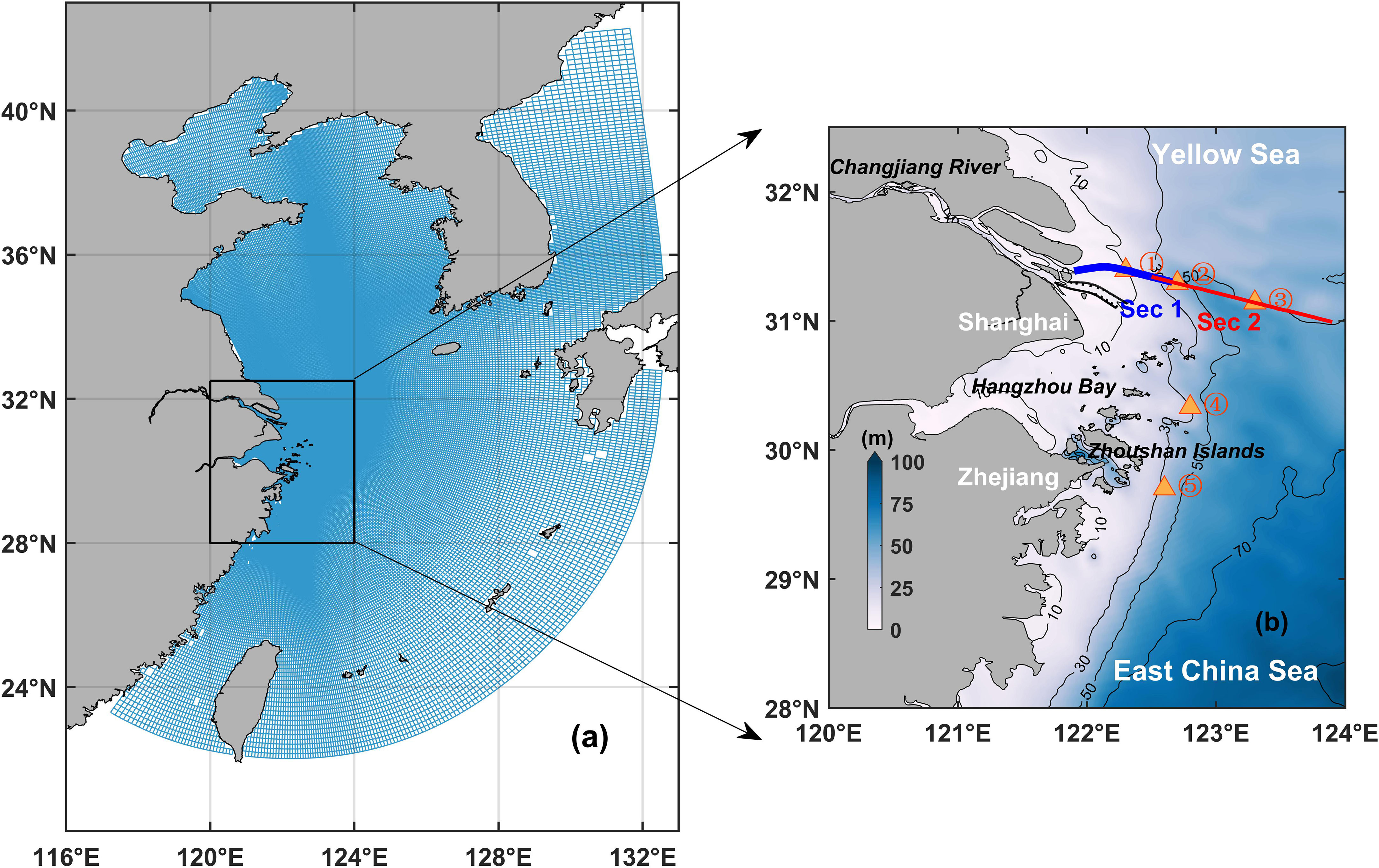
Figure 1 (A) Model horizontal grids. (B) Map of the Changjiang River Estuary and its adjacent water. The solid black lines represent the isobaths (every 20 m from 10 to 90 m). The blue and red lines indicate the representative transects and the five triangles are the representative sites.
The dynamic conditions of the Changjiang River Estuary and its adjacent waters are very complex and are subject to the combined effects of runoff, tides, wind, and other factors. Therefore, numerous related sensitivity experiments were designed to investigate the effects of key physical processes on the distribution of phytoplankton over multiple time scales. All conditions of the control experiment (Case 0) and other conditions of the sensitivity experiments were climatological. All sensitivity experiments with changed conditions were hot-run in the third year (full-year run started from January or flood-season run started from July). The details of the model settings are shown in Table 1.

Table 1 Information regarding the numerical experiments.
Case 1 was designed without tidal forcing, maintaining all the other conditions consistent with control experiment. The results of this case could give us a background variations of chlorophyll without tide.
Case 2 was designed with a 7-day tide delay compared to the control experiment, while maintaining all the other conditions consistent with control experiment, to distinguish distribution and variation such as phytoplankton and nutrients between cases during spring and neap tides (Case 0 and Case 2).
The Changjiang River carries a large amount of freshwater and terrestrial materials, which have a significant impact on the outbreak of phytoplankton blooms in the estuary area and its adjacent waters. Numerous extreme weather events have affected the Changjiang River in recent years, resulting in either extremely high or low discharges (Figure 2A), specifically in the cases of large floods and droughts, respectively. Such differences in the amounts of freshwater and nutrients have influenced the hydrodynamic conditions of the study area to different degrees, with varying effects on the intensity and scale of phytoplankton blooms. Therefore, two more sensitivity experiments, Case 3 and Case 4, were set up, in which the Changjiang River discharge increased and decreased by 50%, respectively, based on the control experiment.
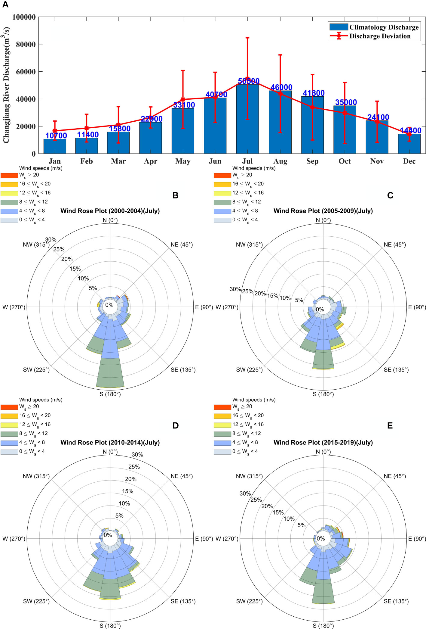
Figure 2 The climatological conditions of Changjiang River discharge and summer monsoon in the Changjiang River Estuary. (A) The climatological (from 1950 to 2016) monthly Changjiang River runoff and its deviation in recent five years. Wind rose diagram in July for the periods of (B) 2000–2004, (C) 2005–2009, (D) 2010–2014, and (E) 2014–2019.
Atmospheric conditions play an essential role in the occurrence of phytoplankton blooms. Wind speed and wind direction have not been stable in recent years, and the northerly winds in summer have not been accidental (Figures 2B–E). Southeasterly winds are predominant for most of July in the Changjiang River Estuary and its adjacent waters in summer, except for a small area where southwesterly winds prevail. As global warming increases, typhoons are occurring more frequently and are characterized by higher wind speeds (Bhatia et al., 2018). Changes in the wind field are often accompanied by variations in the vertical mixing of the water column, which modify nutrient distribution patterns and other conditions, thus indirectly affecting the growth and distribution of phytoplankton and the occurrence of phytoplankton blooms. Therefore, in the next two experiments, Case 5 and Case 6, different wind speeds during the flood season were simulated to investigate the effect of summer wind speed on phytoplankton blooms.
A last set of experiments, Case 7 to Case 20, along with Case 3 and Case 5 which mentioned previously were designed to establish the effects of the time scales of dynamic processes on phytoplankton blooms.
In this study, the “probability of phytoplankton blooms” was used as an index to describe the scale and degree of the chlorophyll maximum in a specified period. The probability of occurrence was calculated as follows:
where Ai represents the serial number of the statistical unit in the study area; and are the start and end times of the participation statistics, respectively; and is the occurrence probability of phytoplankton blooms, which was defined by the following equation:
where is the defined high chlorophyll concentration threshold, i.e., 5 mg/m³ (Korb et al., 2004; Sòria-Perpinyà et al., 2021).
The EOF was used for the analysis of the daily chlorophyll values obtained from the model to understand the intra-annual spatiotemporal variability of chlorophyll distribution. The EOF, also known as principal component analysis, is a common method applied in mathematical statistics to analyze random variables (Wei, 2007). It is particularly useful for the analysis of spatial and temporal patterns in elemental studies and is commonly used in marine and atmospheric sciences (Thompson and Wallace, 1998; Storch, 2001).
The key indices of the horizontal chlorophyll maximum in different sensitivity experiments (i.e., area proportion, mean value, and offshore distance) were calculated to determine the response time of phytoplankton distributions to physical processes. The area proportion was calculated as follows:
where represents the area with a chlorophyll concentration greater than 5 mg/m3, t represents time, and A represents the study area. The mean value is the average chlorophyll in areas with chlorophyll concentrations greater than 5 mg/m³. The offshore distance is the average distance between area with chlorophyll concentrations greater than 5 mg/m³and position (122°E, 31°N).
The phytoplankton bloom events reported in the study area between 2000 and 2014 are summarized in Figure 3. A total of 192 blooms were recorded, with the highest number being recorded in 2006 and largest area of occurrence being recorded in 2005, accounting for 14.1% of the total number of events and 25.1% of the total area of events, respectively. These results suggested that there was a considerable inter-annual variation in the occurrence of phytoplankton blooms. In addition, a clear intra-annual variation in distribution was also observed. Phytoplankton blooms mainly occurred in spring and summer throughout the year. The three most frequent outbreak months between 2000 and 2014 were May, June, and July, with 92, 58, and 12 events, respectively, which accounted for 84.4% of the total events (Figure 3B). Throughout the period examined, phytoplankton blooms on average were mainly distributed within the 30-m to 50-m isobaths to the south of the Changjiang River Estuary (Figure 3A). The timing and location of bloom events varied within the study area: the events in the southern part occurred earlier, while those in the northern part occurred later.

Figure 3 Statistics of harmful algal bloom events data during the 2000–2014 period. (A) Distribution, (B) monthly frequency, and (C) monthly duration and cumulative scales of recorded phytoplankton blooms. The frequency of phytoplankton blooms corresponding to each duration was marked with red numbers.
In addition, the duration of outbreaks, which consisted of a rapid development and consequent recession, also indicated phytoplankton variations over shorter time scales. It can be referred as event-scale variations. It shows that most of the phytoplankton blooms lasted< 10 days, with durations of 1 day, 2 days, and 3 days being the top three most frequent and accounting for 53.6% of the total. However, the accumulated area of events showed two peak frequency states at durations of 1 day and 7 days which can essentially represent the variation of blooms at the weekly and daily time scales. This result indicated that outbreaks lasting for 7 days covered a larger area. At the same time, the durations and areas covered in June and July were shorter and smaller, respectively, than those in May. This was especially the case in July, when most of the blooms lasted for 3 days or less covering an area smaller than 500 km2.
The results of the numerical model were used to further analyze phytoplankton variability. Seasonal variations in chlorophyll were analyzed based on the monthly average surface chlorophyll concentration and the probability of phytoplankton blooms in representative months in the control experiment (Equations 1, 2; Figure 4). The results showed that the monthly surface chlorophyll values were high in spring and summer (represented by April and July, respectively, Figures 4B, C), decreased in autumn (represented by October, Figure 4D), and remained low in winter (represented by January, Figure 4A). Phytoplankton blooms started to appear sporadically in April, peaked in July, and then started to decrease, receding and shrinking in October, and almost disappeared in January. The horizontal chlorophyll maximum region was located between 122°E and 123°E, parallel to the coastline, and appeared as a long, curved, and oscillating strip with small patches from the northeastern to the southern end of the Changjiang River Estuary. The results obtained from the numerical model showed that the bloom distribution patterns were consistent with the phytoplankton bloom records.
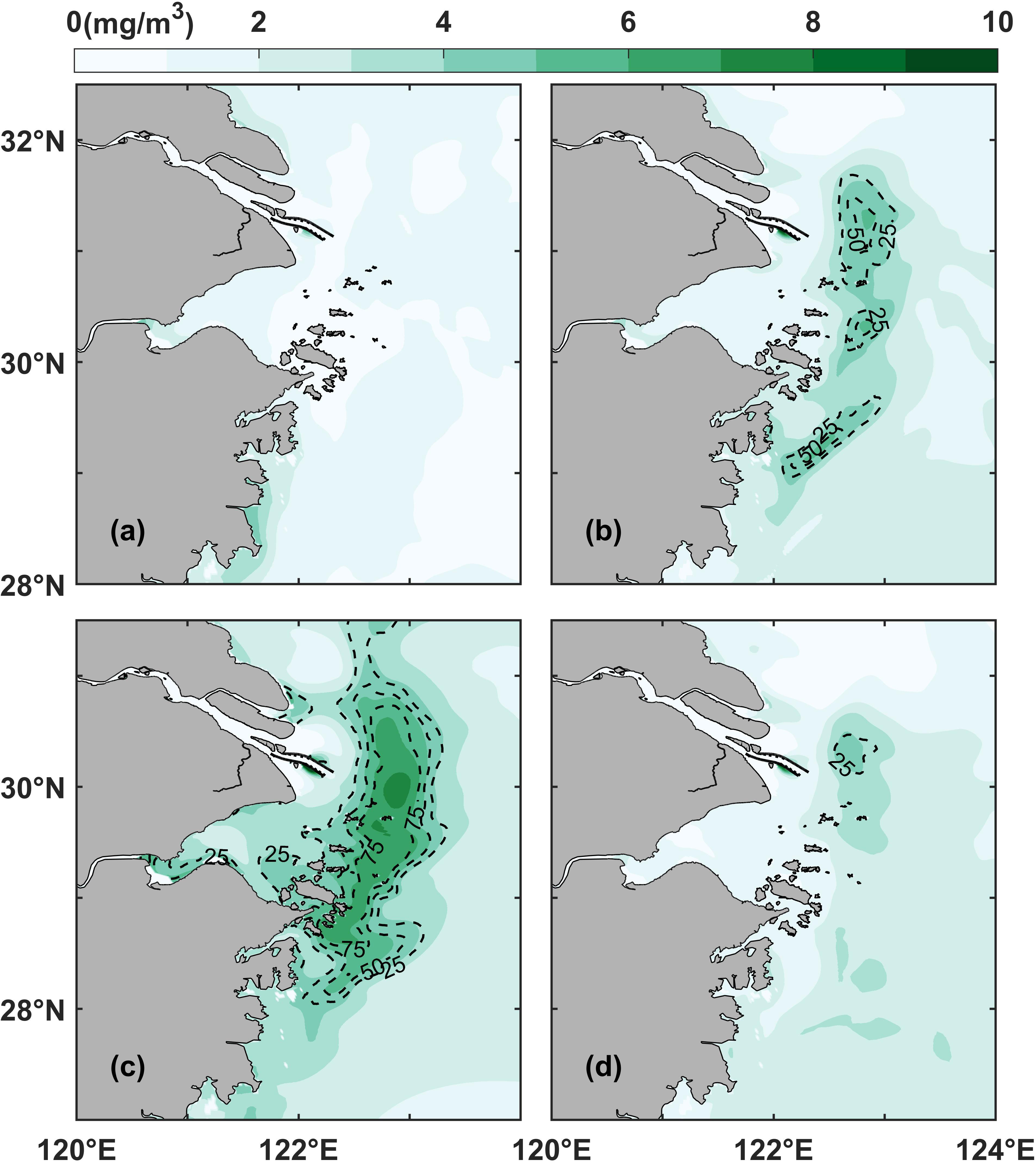
Figure 4 Surface monthly average chlorophyll distribution in the control experiment (Case 0): (A) January, (B) April, (C) July, and (D) October. The dotted black lines represent the distribution of the probability of phytoplankton blooms.
It should be notable that our numerical model results showed the highest biomass in July (Figure 4) while the results of phytoplankton bloom events (Figure 3) showed the highest frequency in May and June. This discrepancy was largely due to the seasonal succession of predominate algae species in the study region (Tang et al., 2006; Yang et al., 2014). The complex biological processes including grazing and species competitions increased the simulation difficulty. Even so, previous field investigations demonstrated that the highest biomass emerged in summer season in the study region (Yang et al., 2014). The discrepancy was beyond the main purpose of this study.
Indeed, besides the seasonal variations, the horizontal chlorophyll maximum region also has variations within monthly scale. The monthly probability of phytoplankton blooms computed by the model showed that the horizontal chlorophyll maximum region varied significantly over periods shorter than one month (Figure 4). For instance, some identified horizontal chlorophyll maximum region in April only had the value of 50% probability of phytoplankton blooms (Figure 4B). Even in July, the core region of probability could not reach 100% (Figure 4C), implying that the horizontal chlorophyll maximum region varies at the spatiotemporal scale, i.e., by oscillating in space, growing and declining over short time scales.
The daily averaged chlorophyll time series at five sites (shown in Figure 1B) in control experiment (Case 0) were selected to further analyze the variation of phytoplankton biomasses in the Changjiang River Estuary at more specific time scales. These sites were arranged either across or along the shelf to represent spatial differences in both directions (Figure 1B). The hourly chlorophyll data at each site from April to September in Case 0 and Case 1 were also spectroscopically analyzed to determine the main time scale of phytoplankton variation.
In general, the spectroscopic analysis of all five sites in control experiment detected periods of approximate half a day, one week, and one fortnight, corresponding to the signals of flood-ebb, half-spring-neap, and spring-neap cycles (red lines in Figures 5F–J). However, the results with tidal closure showed significantly weakened periodic signals (sky blue lines in Figures 5F–J). Only periods of shorter than half a day, and one week was detected, while the period of one fortnight was missing. These periodic signals of chlorophyll variations without tide were corresponded to the signals of diel solar irradiation and inherent periodic signals of chlorophyll variations. The daily averaged chlorophyll time series showed that the periodic signals of approximately one fortnight owned large amplitudes, while those of one week presented small fluctuations (Figures 5A–E, also seen in Supplementary Figure S1). This implied that the spring-neap tidal variability dominated phytoplankton variations over the time scale of days in spite of some inherent minor fluctuations of the half-spring-neap cycles.
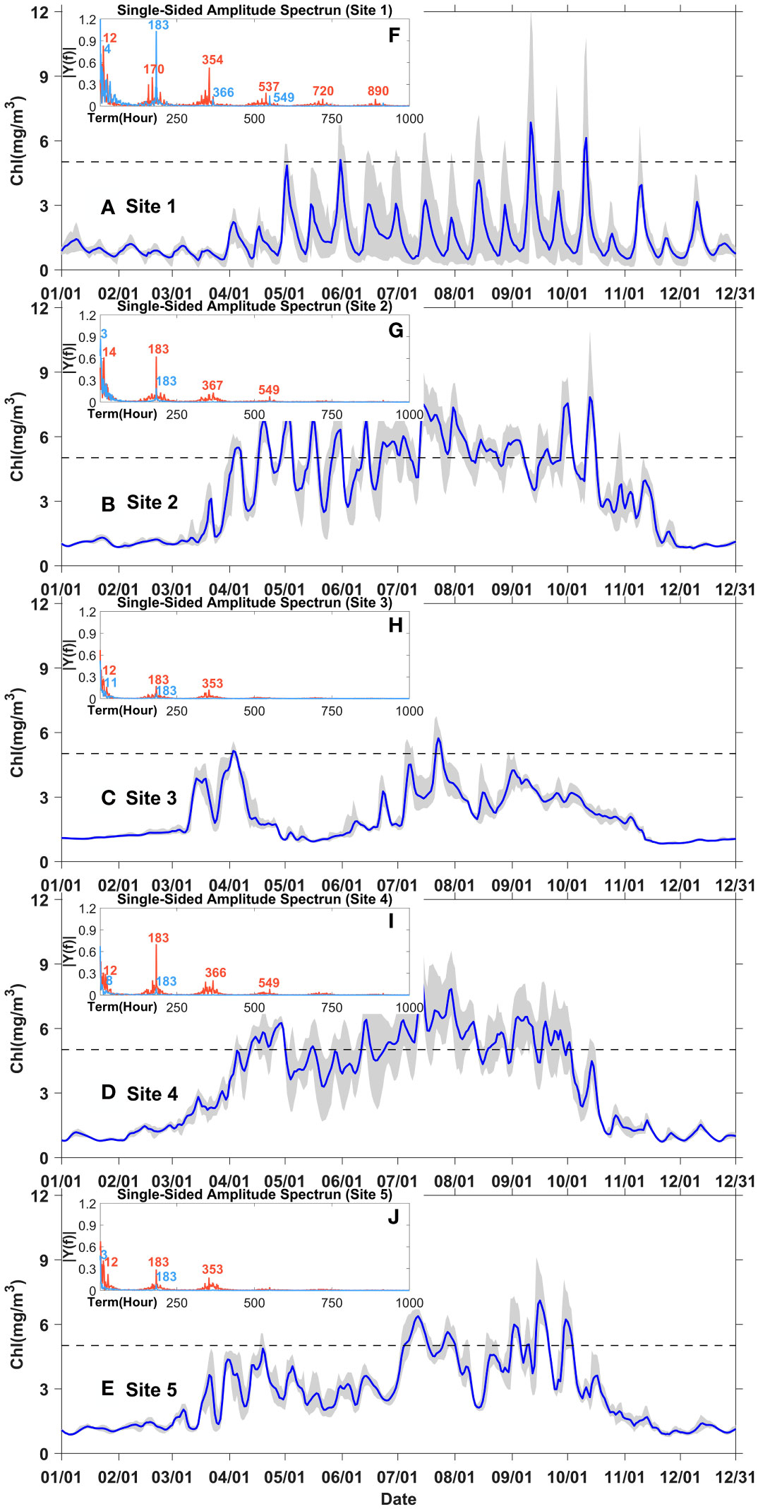
Figure 5 Year-around time series of chlorophyll concentration at site 1-5 in the control experiment (Case 0) (A–E); spectral analysis of hourly chlorophyll at site 1-5 from April to September in Case 0 (red) and Case 1 (sky blue) (F–J). Grey shading represents the chlorophyll range over the day. The blue lines represent the daily averaged chlorophyll concentration.
The time-series data at sites 1 to 3 showed the differences in phytoplankton biomass across the shelf. These positions also crossed the horizontal chlorophyll maximum region east of the Changjiang River mouth, an area where both onshore and offshore variations in phytoplankton biomass can be observed. In spring and summer, the data at site 1 showed significant high value of phytoplankton with obvious variations (grey shade), while that at site 2 showed longer phytoplankton blooms, indicating that more distinct event-scale variations occurred onshore than offshore and more distinct phytoplankton blooms occurred offshore than onshore in the horizontal chlorophyll maximum regions (Figures 5A, B). That at site 3 showed the smallest variation and seldom high value of phytoplankton (Figure 5C), indicating that phytoplankton seldom blooms in this region. Moreover, the results of spectroscopic analysis demonstrated that the period signal was stronger onshore than offshore in the regions of horizontal chlorophyll maximum. The above results implied that 1) in the regions of the chlorophyll maximum, phytoplankton blooms statistically lasted longer offshore than onshore, and 2) phytoplankton blooms onshore occurred relatively periodically while those offshore occurred randomly (Figures 5F, G).
The spectroscopic analysis of site 2, 4, and 5 revealed the differences along the shelf. At these sites, from north to south, were also located small patches of the chlorophyll maximum region. The results showed that the daily variance signals became stronger when chlorophyll value sustained in high levels at the north two sites (site 2 and site 4). For instance, the shaded area was larger in June and July than in April and May at both Points 2 and 4; however, the signal was not significant at Point 5 (Figures 5B, D, E). The above results suggested that the chlorophyll maximum regions that were close to the Changjiang River Estuary exhibited more significant event-scale variabilities. Furthermore, variations occurred over short time scales in spring and summer, which was also consistent with the results shown in Figure 3C indicating that the durations of phytoplankton bloom events were last for days from May to July.
Both the records of the phytoplankton bloom events and the numerical model results demonstrated that phytoplankton biomass varied spatially over multiple time scales, from the seasonal to the weekly and daily scales. To reveal the regularity of chlorophyll variations over multiple time scales in the whole study area, the EOF was then used for further analysis of the numerical model results. The analysis was based on the daily averaged chlorophyll concentrations of the model, and three main EOF modes were calculated, each of them accounting for 47.3%, 17.7%, and 7.9% of the total chlorophyll variation rate, i.e., 72.9% of the total variation rate (Figure 6). This meant that the three main modes could represent the chlorophyll variation in the Changjiang River Estuary and its adjacent waters. The area with high standard deviation of chlorophyll was mainly located between the 30-m and 50-m isobaths, which corresponded to the usual location of the horizontal chlorophyll maximum region.
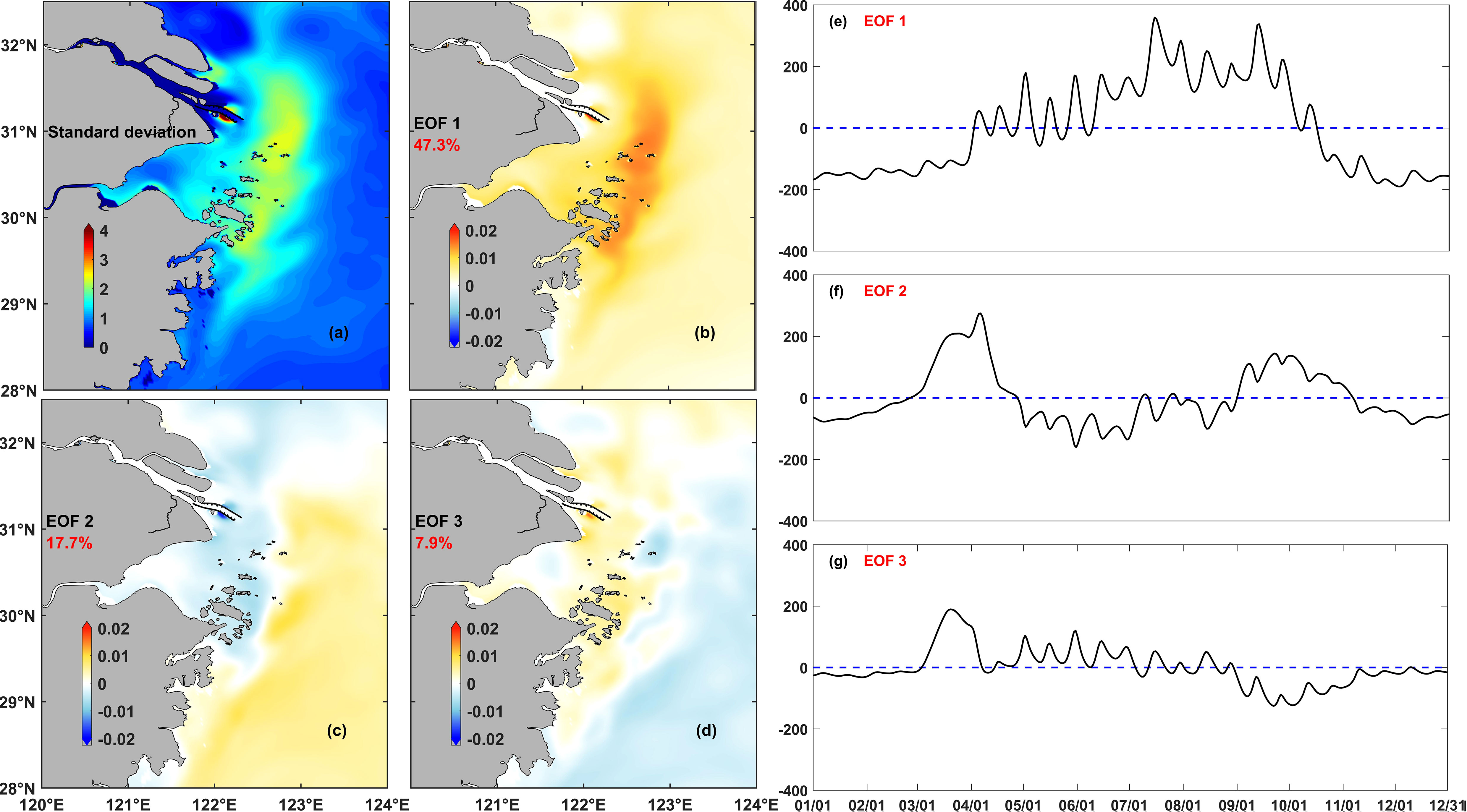
Figure 6 Results of the EOF analysis of daily average chlorophyll in the control experiment (Case 0): (A) standard deviation, (B–D) spatial coefficients for each mode, and (E–G) temporal coefficients for each mode in Case 0, the dotted lines denote the zero baseline.
The variance contribution rate of mode I was 47.3%, which represented the most dominant trend of chlorophyll variation and reflected the main characteristics of the seasonal variation of phytoplankton. Spatially, the horizontal chlorophyll maximum region extended to 30°N and south of the area. Based on the variation of the temporal coefficients, this region was characterized by significant seasonal variation. The horizontal chlorophyll maximum region outside the Changjiang River Estuary in spring and summer was the most dominant distribution characteristic of phytoplankton in this area. This region began to form in May and lasted until the end of September. However, the temporal coefficients also fluctuated over the time scale of weeks.
The variance contribution rate of mode II was 17.7%. This mode described the evolution of the horizontal chlorophyll maximum region, from generation to recession. The phytoplankton biomass first grew along the Zhejiang coast and the shelf area outside the Changjiang River Estuary in April and gradually gathered northward along the coast to form a horizontal chlorophyll maximum region, which started to decline toward the shelf and southward in August.
The variance contribution rate of mode III was 7.9%. This mode mainly showed the strong spatial oscillation of the horizontal chlorophyll maximum region over the time scale of days. It also showed that these regions extend onshore or offshore, and the intensity of these regions decreased or increased over this time scale. The temporal coefficients of modes II and III were also shown to be more likely to change its positive-negative sign in summer than in spring, indicating that phytoplankton was more likely to vary over short time scales in summer than in spring.
Both the records of phytoplankton bloom events and the chlorophyll concentrations simulated by the numerical model suggested that phytoplankton varied significantly in the Changjiang River Estuary region within one year over multiple time scales. Since the region is affected by various dynamic processes, it was considered worthwhile to explore the relationships between them and phytoplankton variability. To this end, a series of sensitivity experiments were designed to investigate the effects of key processes. The detailed experimental settings were introduced in the Methods section and Table 1.
Both the time series of the modeled chlorophyll concentrations and the results of EOF analysis showed that the phytoplankton distributions presented high-frequency and stable oscillating signals (Figures 5, 6). The results of spectroscopic analysis also showed that the stable signals had periods of approximately half a day and a fortnight (Figures 5F–J), which corresponded to the flood-ebb and spring-neap tidal cycles in the study area. Thus, the frequency of these chlorophyll variations should be strongly influenced by tidal forcing.
The first two sensitivity experiments (Case 2 and Case 0) examined chlorophyll variability during the spring-neap tidal cycles. The results showed that the phytoplankton bloom probability was generally higher in Case 2 than in Case 0 (Figure 7D), specifically on the onshore and offshore sides of the chlorophyll maximum regions. These results indicated that phytoplankton blooms during spring tide probably occurred in a smaller region compared to those during neap tide. As the tidal cycle periods were relatively stable, the phytoplankton variations during different tidal cycles could be regarded as intrinsic, which were assisted in exploring the effect of other dynamic processes.
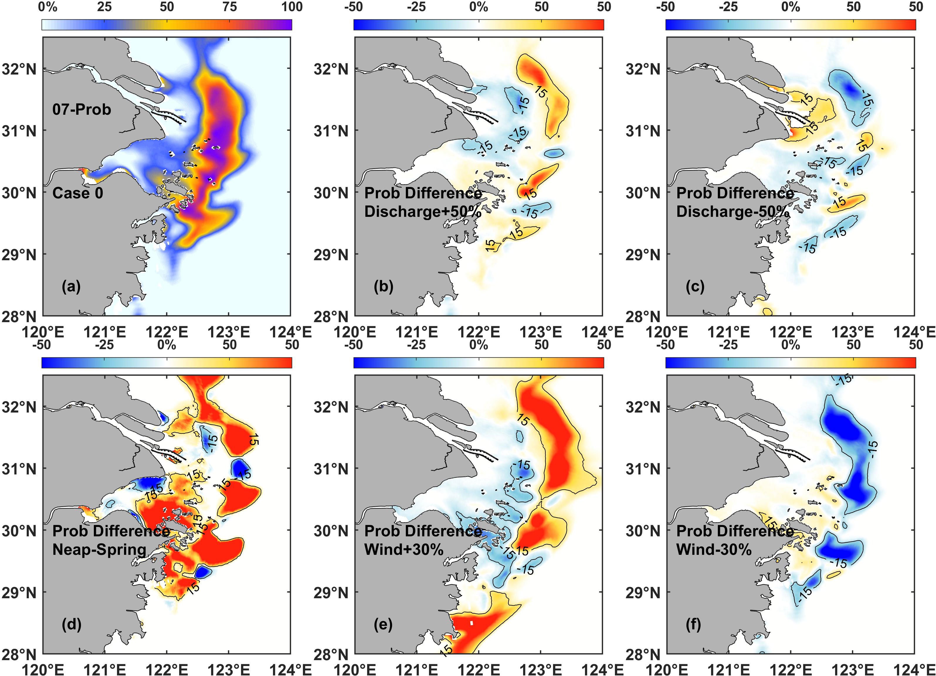
Figure 7 (A) Surface probability distribution of phytoplankton blooms in the control experiment (Case 0). Difference in the surface probability in July between Case 0 and each of the following: (B) discharge sensitivity experiment Case 3, (C) discharge sensitivity experiment Case 4, (D) tidal sensitivity experiment Case 2, (E) wind sensitivity experiment Case 5, and (F) wind sensitivity experiment Case 6.
The runoff of the Changjiang River is a key dynamic process controlling the hydrological and environmental conditions in the estuarine region. The second and third sensitivity experiments (Case 3 and Case 4) examined chlorophyll variability under the increase and decrease of runoff during the flood season, respectively. The results showed that the increase and decrease of the Changjiang River discharge during flood season could produce opposite impacts on phytoplankton variation (Figures 7B, C). In the case of increasing runoff (Case 3), the probability of phytoplankton bloom occurrences largely increased on the offshore side of the chlorophyll maximum region and decreased on the onshore side. The opposite was observed in the case of decreasing runoff (Case 4).
A number of spatial differences in the probability of bloom events due to the effect of runoff were also detected, and they were more significant in the northern parts than in the southern parts of the study area. For instance, the variant values of probability were higher in the region around site 2 and 4, and lower in the region around site 5. These results suggested that the intensity of influenced area by runoff was gradually weakened as the distance prolonged from the river source. Furthermore, the influence on the southern parts adjacent to the Changjiang River Estuary was also weaker than that on the northern parts during summer season.
Wind is another key element affecting dynamic processes in riverine environments. The fourth and fifth sensitivity experiments (Case 5 and Case 6) examined chlorophyll variability under the increase and decrease of the prevailing summer monsoon, respectively. The results showed that under the condition of increased summer monsoon (Figure 7E), the probability of phytoplankton blooms increased in the core and offshore side of the chlorophyll maximum region, while it decreased on the onshore side. However, the decrease in value was smaller than the increase in value. This implied that the enhanced wind conditions stimulated the occurrence of phytoplankton blooms and favored the shifting of the chlorophyll maximum region offshore. In contrast, as the summer monsoon declined (Figure 7F), the probability of phytoplankton blooms at the core of the chlorophyll maximum region decreased. However, the affected region in this case was not as large as that under the enhanced wind conditions (Figure 7E), specifically at the southern edge of the study area. The region with an increased probability of phytoplankton blooms on the onshore side of the chlorophyll maximum region in Case 6 was also not obvious, which implied that the reduced wind conditions were not conducive to the maintenance of phytoplankton blooms.
The results of the above sensitivity experiments revealed that the variation of physical processes occurring within the estuarine waters induced comparable changes in phytoplankton distribution. However, in reality, multiple physical processes vary simultaneously, and their joint influences were therefore further investigated. To this end, more sensitivity experiments were conducted setting different runoff and wind pulses over different time scales (3, 7, 15, and 30 days) starting from spring or neap tides, and the key indices (area proportion, mean value, and offshore distance) of the horizontal chlorophyll maximum regions were calculated (mentioned in Section 2.4.3 and Equation 3).
The above-mentioned key indices showed an obvious inter-tidal variability (Figures 8, 9). Area proportion and mean value increased, while offshore distance decreased from spring to neap tide (the grey lines in Figures 8, 9). The opposite trends were observed from neap to spring tide. The obtained values indicated that the horizontal chlorophyll maximum developed and migrated offshore from spring to neap tide, while it receded and migrated onshore from neap to spring tide. Runoff and wind pulses also superposed effects on the horizontal chlorophyll maximum starting from spring tide or from neap tide. We used the differences of value of above-mentioned key indices between sensitivity experiments and control experiment to denotes the response of key indices. It would be elaborated below.
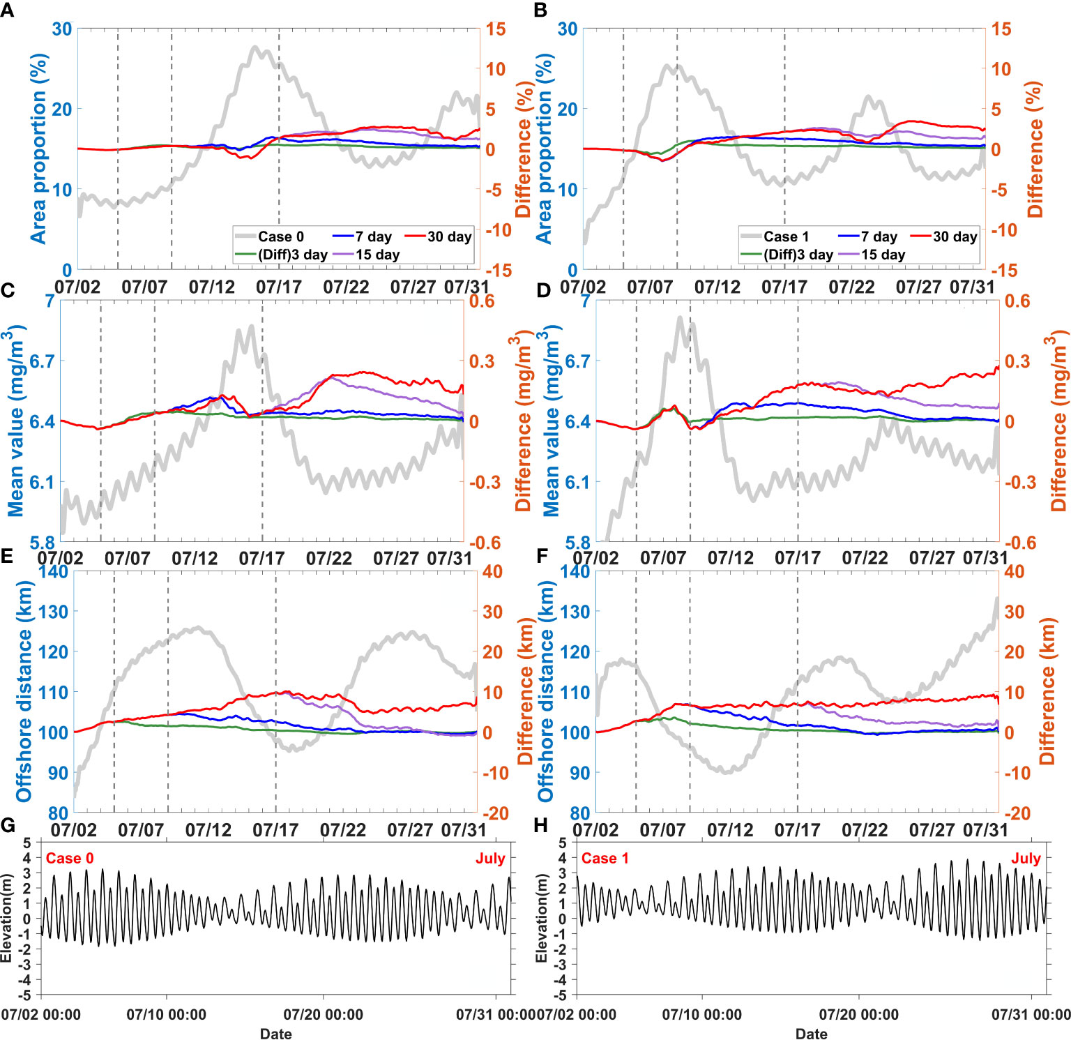
Figure 8 Difference between the control experiment (Case 0) and discharge disturbance experiments (Case 7-9), difference between Case 2 and discharge disturbance experiments (Case 10-12) for area proportion (A, B), mean value (C, D), and offshore distance (E, F), elevation fluctuation of Case 0 and Case2 (G, H), respectively. The solid grey lines represent results of the control experiment (Case 0) and Case 2. The dotted grey lines represent the end of the 3, 7 and 15 day disturbances, respectively.
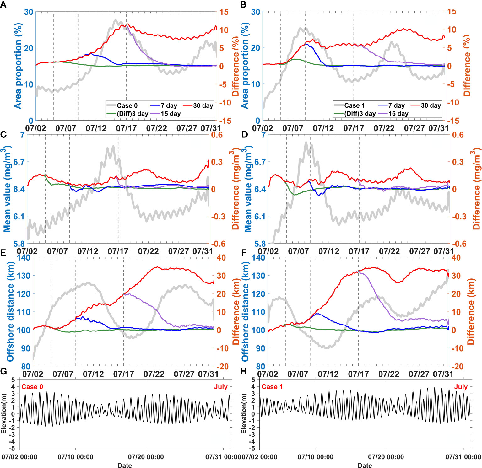
Figure 9 Difference between the control experiment (Case 0) and wind disturbance experiments (Case 14-16), difference between Case 2 and wind disturbance experiments (Case 17-19) for area proportion (A, B), mean value (C, D), and offshore distance (E, F), elevation fluctuation of Case 0 and Case2 (G, H), respectively. The solid grey lines represent results of the control experiment (Case 0) and Case 2. The dotted grey lines represent the end of the 3, 7 and 15 day disturbances, respectively.
When the runoff pulses increased during spring tide, the response of area proportion took more than 10 days (Figure 8A); in contrast, when they increased during neap tide, the response occurred in less than 5 days (Figure 8B). These sensitivity experiments (Case 3, Case 7-Case 13) involving increased runoff pulses showed that the responses of area proportion were always negative during neap tide when the horizontal chlorophyll maximum developed. These responses gradually shifted and became positive when the horizontal chlorophyll maximum receded. This situation only happened when the runoff pulses could last until the phytoplankton blooms developed from spring to neap tides. Otherwise, the negative response would gradually disappear or even never emerge.
The response of mean value was different from that of area proportion (Figures 8C, D). In all the sensitivity experiments with increased runoff pulses, the mean values showed a slightly negative response during the first 3 days. After this time, the mean values began to show a positive response, which lasted up to 2–4 days after the runoff pulses ended. Specifically, this delayed positive response was slightly stronger than that occurring during the runoff pulses.
The response of offshore distance to runoff was always positive. All the sensitivity experiments showed an integrated increased response of offshore distance (Figures 8E, F). The variations of offshore distance gradually recovered when the runoff pluses ended. Indeed, the offshore distance would not persistently increase, it maintained a relatively stable value after 7–15 days of runoff pluses even if the pluses still sustained.
When wind pulses increased during spring tide 5 days were required for the response of area proportion (Figure 9A). In contrast, when they started during neap tide, the response took less than 5 days (Figure 9B). The area proportion showed mostly positive responses during neap tide when it increased and reached its maximum. This occurred even when the wind pulses ended before the maximum area proportion was reached; for instance, in the case of wind pulses lasting for over 7 days during spring tide and over 3 days during neap tide.
The response of mean value was more rapid than that of area proportion (Figures 9C, D). The results showed immediate positive responses of mean value within the first 2 days. Subsequently, it slowed down and fluctuated, and remained stable for about 2 weeks if the wind pulses persisted. Once these ended, the positive response of the mean value would also recover to normal in 1 or 2 days.
The response of offshore distance was also mono-positive. The rapidly increasing response of offshore distance occurred in 4–6 days and could be maintained for 5 more days if the wind pulses persisted (Figures 9E, F), but it decreased when the wind pluses ended. The periods of rapidly increasing response also matched the timing of the horizontal chlorophyll maximum extending offshore. Offshore distance also did not persistently increase; it remained relatively stable during wind pulses (for 15–22 days) and even after they ended.
Although the increased runoff and wind caused similar variation patterns in the horizontal chlorophyll distribution, differences were observed in relation to the time scale. For example, the effect of wind was faster than that of runoff (Figures 8 and 9). All of the three indices (area proportion, mean value, and offshore distance) of the horizontal chlorophyll maximum responded more rapidly to wind than to runoff. The responses to wind pulses occurred a few days earlier and were stronger than that to runoff. At the same time, the periods of recovery were shorter when the wind pulses ended than when the runoff pluses ended. Another difference was that delays were observed more for the runoff effects than for the wind effects. For instance, the response of mean value was noticeably delayed when the runoff pulses were over (Figures 8C, D), but such delay was not observed when the wind pulses ended (Figures 9C, D).
Estuarine and coastal regions are located at the interface between land and ocean and are influenced by dynamic processes such as tide, runoff, and wind. The spatiotemporal variations of the hydrodynamic and ecological environments are very complex, exhibit strong nonlinear interactions, characterizing as rapid changes over short time and small space scale (Ge et al., 2020). The previous sections investigated and reproduced the variability of phytoplankton blooms and chlorophyll distributions over multiple time scales. Many sensitivity experiments were designed to explore the influence of dynamic processes and their time scales. The dynamics mechanisms of phytoplankton variation underlying these results need to be further discussed.
Both the phytoplankton bloom records and numerical modeling data showed that the regions with high phytoplankton concentrations located at particular positions along the coast varied over intra-annual or shorter time scales. For example, this was reflected by the fact that 1) most bloom events lasted for 1–7 days at these particular coastal positions (Figure 3C); 2) the simulated probabilities could not reach 100% even in the season with the highest frequency of phytoplankton blooms (Figure 4); and 3) the time series and EOF analysis revealed oscillating signals of variability over the time scale of days (Figures 5, 6).
These oscillating signals corresponded to the periods of spring-neap tidal cycles (Figures 5, 6), implying that they were controlled by tidal forcing. In macrotidal estuarine and coastal regions, tidal forcing is considered as one of the major processes determining the short time scale variations of many processes. It was shown not only to regulate the transport of different materials, for example via tidal dispersion or flat-trough exchange (Lucas et al., 1999; MacCready, 2004; Fram et al., 2007), but also to significantly control the phytoplankton growth–loss balance, for example through nutrient input or resuspension of benthic biota during spring-neap tide (Cloern et al., 1989; Lucas and Cloern, 2002; Ha et al., 2020; Yelton et al., 2022). It should be noted that the tide-related factors affecting phytoplankton vary in different estuaries depending on their geometry, biota, and hydrological conditions (Cloern et al., 1989; Hickey et al., 2010). Our previous study of the tidal mechanisms of phytoplankton variability in the Changjiang River Estuary suggested that the river–tide interactions induced the improved light availability and activated more fluvial nutrients as well as the extension of the phytoplankton plume front further offshore from spring to neap tide (Wang et al., 2023). The interactions during this period were shown to not only stimulate phytoplankton blooms, but also expand the region of the horizontal chlorophyll maximum on both the offshore and onshore sides. Onshore, the river–tide interactions improved light availability due to the inhibition of sediment resuspension allowing more fluvial nutrients to be available for phytoplankton consumption. Offshore, the interactions further extended the plume front in the offshore direction, also expanding the horizontal chlorophyll maximum. In the present study, the area proportion and mean value of the horizontal chlorophyll maximum in the control experiment confirmed the tidal effects described above (Figures 8, 9).
In addition, other dynamic processes were also suggested to regulate phytoplankton variations. Previous studies have shown that river discharge variations not only changed their residence time in estuaries (Odebrecht et al., 2015), which further influenced phytoplankton aggregation, but also regulated hydrological conditions such as the supply of fluvial nutrients (Paerl et al., 2010), which affected phytoplankton growth. In the highly turbid Changjiang River Estuary, the river discharge load forms the river plume, which, together with its front structure, was suggested to be dynamically correlated with the critical boundary of the horizontal chlorophyll maximum (Wang et al., 2019a and Wang et al., 2019b; Ge et al., 2020). For example, according to estuarine dynamics, the variation of river discharge, such as an increased runoff pulse, pulls the plume front offshore (Beardsley et al., 1985), and also extends the horizontal chlorophyll maximum offshore. At the same time, given the constant fluvial nutrient concentration, the increased discharge also loads more nutrients into the estuary. This greater supply promotes phytoplankton growth, which in turn enhances the scale of bloom events. The integrated difference of probabilities and the three indices (area proportion, mean value, and offshore distance) of the horizontal chlorophyll maximum detected in the sensitivity experiments demonstrated the above mechanisms regulated by runoff variations (Figures 7, 8). The vertical distribution of salinity, chlorophyll, and sediment observed in Case 0 and Case 3 further illustrated the effects of runoff on phytoplankton (Figure 10). The increase of runoff caused the bottom front of the river plume to move significantly offshore and the consequent extension of the horizontal chlorophyll maximum region (Figures 10A–F).
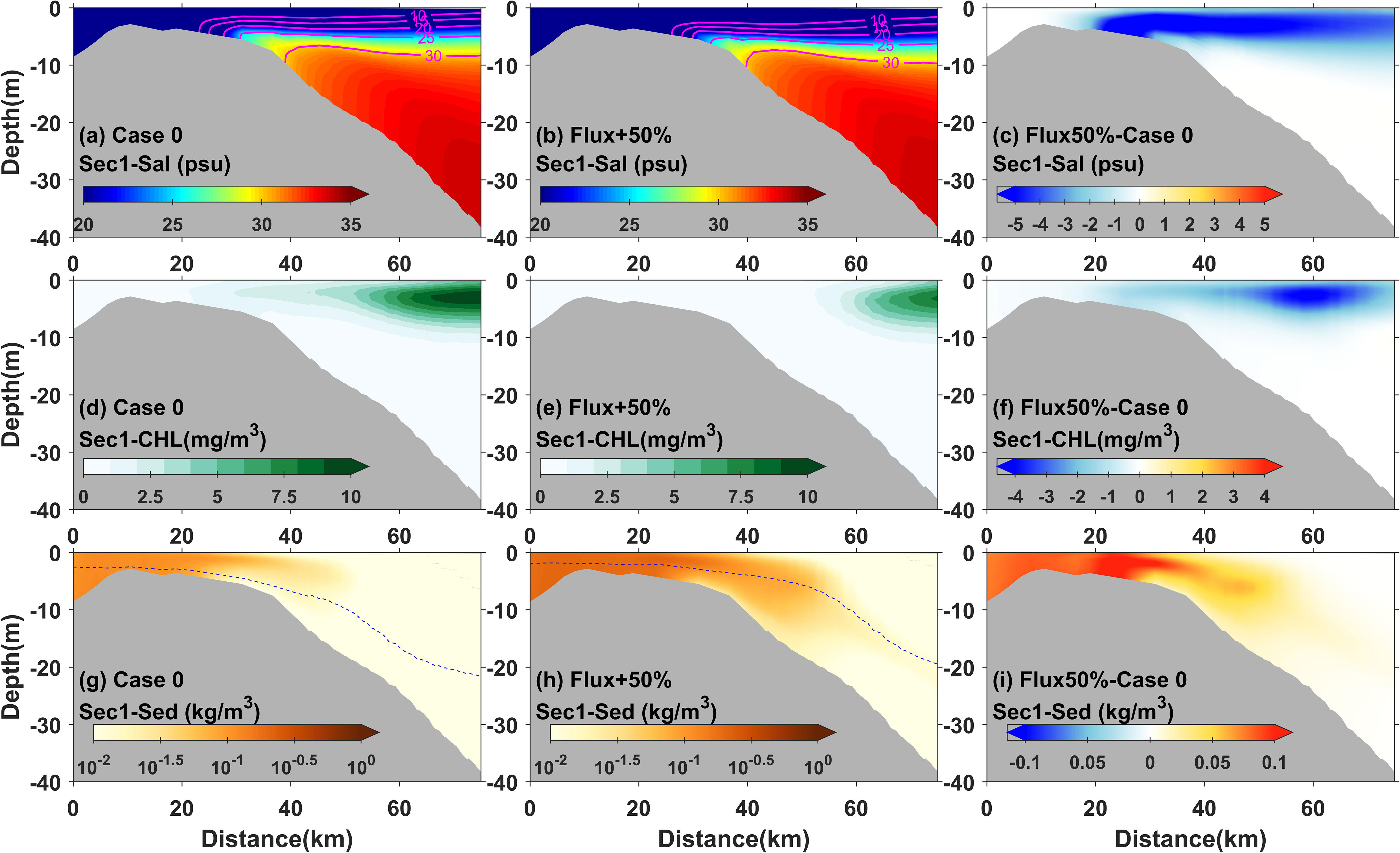
Figure 10 Modeled 3-day averaged salinity (A, B), chlorophyll (D, E), and suspended sediment concentration (G, H) and their differences (C, F, I), respectively, in transect 1 for Case 0 and Case 3 during neap tide. The dotted blue lines represent the euphotic depth.
Wind is also a critical factor that influences phytoplankton dynamics. Previous studies have suggested that wind significantly regulates the vertical dynamics in estuaries through vertical mixing and upwelling/downwelling processes (Austin and Lentz, 2002) as well as through the induction of horizontal Ekman transport in the upper Ekman layers (Austin and Lentz, 2002). In the Changjiang River Estuary, the southeasterly winds prevailing in summer, favor upwelling, which induces the offshore Ekman transport. On one hand, the increased pulse of the summer monsoon deepened the upper mixing layer and enhanced upwelling, supplying bottom nutrients, especially phosphate, to the surface, where they are limited. On the other hand, the pulse enhanced the offshore Ekman transport, which extended the horizontal chlorophyll maximum offshore. The difference of probabilities, the indices of the horizontal chlorophyll maximum, and the vertical distribution of chlorophyll and nutrients flux observed in the sensitivity experiments demonstrated the above effects exerted by wind variations (Figures 7, 9, 11).
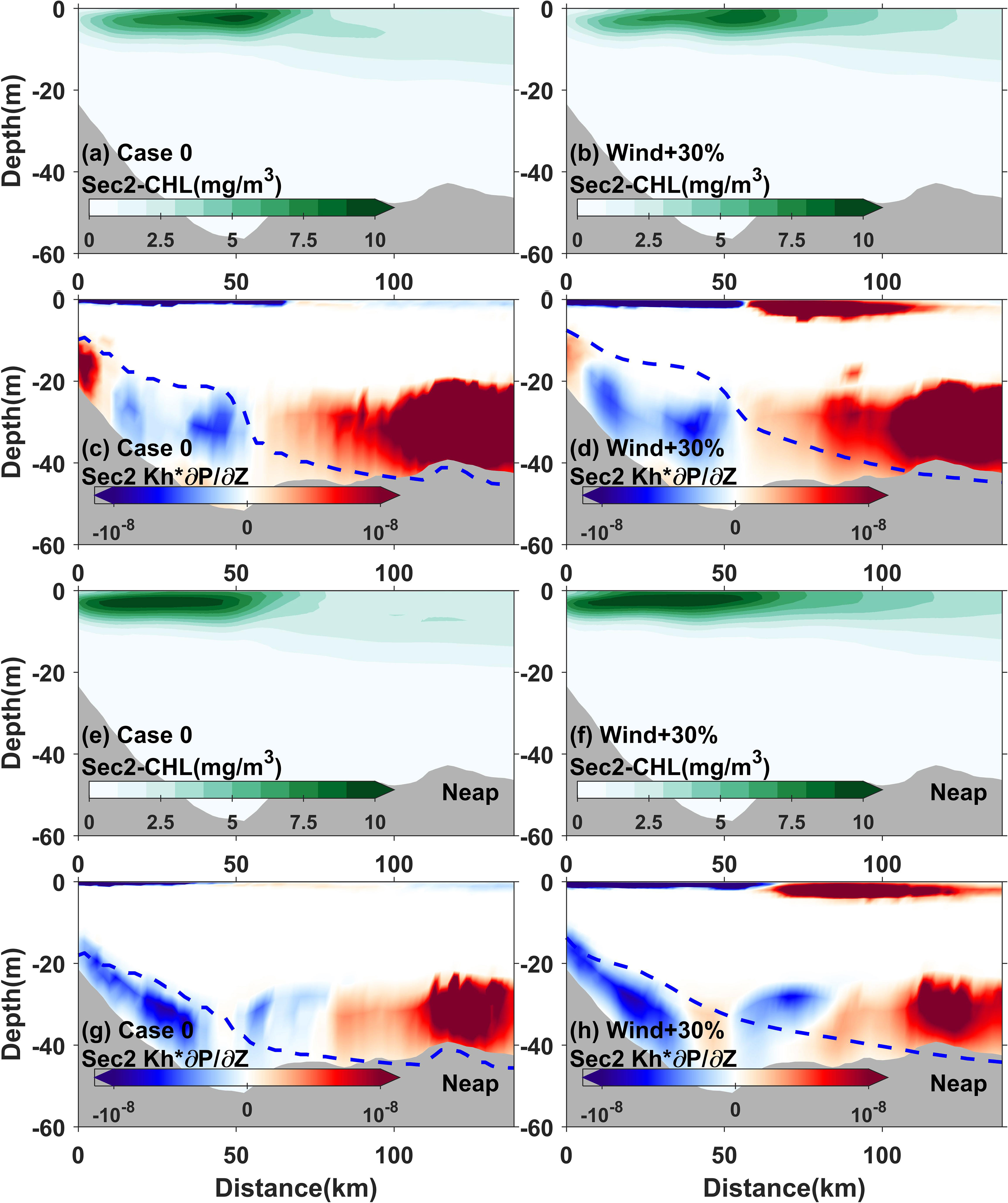
Figure 11 Modeled 3-day averaged chlorophyll (A, B, E, F) and turbulent vertical phosphate flux (Kh*∂N/∂Z) (C, D, G, H) in transect 2 for Case 0 and Case 5 during the time 3 days before neap tide and during neap tide. The dotted blue lines represent the euphotic depth.
Various dynamic processes were shown to influence the spatiotemporal distribution of the horizontal chlorophyll maximum (Figures 7–9). Some of them produced contrasting responses. For example, the increased pulse of runoff shortened the estuary’s residence time and increased the nutrient load at the same time, impeding phytoplankton aggregation and stimulating phytoplankton blooms, respectively. Some dynamic processes induced a bi-directional response, i.e., runoff-tide interactions improve light conditions onshore and extend the plume further offshore from spring to neap tide. These two processes during the spring-neap tidal cycles also induced the bi-directional extension of the horizontal chlorophyll maximum across the shelf from spring to neap tide. Therefore, understanding the temporal scale of these dynamic effects could benefit a more comprehensive for the time of phytoplankton adjustment.
A short time scale corresponding to horizontal motion in hydrodynamics is the transport time of the gravitational wave (Saucier and Chassé, 2000). It is an expressive form of the inertial force. For example, given the geometry of the Changjiang River Estuary, only a few hours would be required to initiate the response of current velocity in the river plume region when a runoff pulse occurs upstream. This response would induce a rapid regulation of the estuarine residence time and further influence phytoplankton distribution (Lucas et al., 2009). The sensitivity experiments with increased runoff pulses made in this study showed an immediate adjustment of the horizontal chlorophyll maximum, i.e., a negative response of mean value and a positive response of offshore distance in the first 3 days (Figures 8C, D). These phytoplankton adjustments should be sort to the response of the gravitational wave. Subsequently, a longer time scale corresponding to the horizontal motion is the time of substances transport such as nutrients. In the Changjiang River Estuary, several days are required to transport nutrients from upstream to the river plume region (Wang et al., 2015). The mean value index demonstrated adverse responses of the gravitational wave after the first 3 days (Figures 8C, D), indicating the effects of phytoplankton and nutrients transported from upstream. In the vertical direction, the mixing effect in estuarine waters occurs within seconds to hours, while the effects of vertical transport and Ekman transport require days (Tian, 2019). In the case of increased wind pulses examined in this study, these effects were shown to induce the rapid responses of mean value and offshore distance within the first 3 days (Figure 9). It is notable that, since the transport of the river discharge and land-derived material require time, the effect of runoff also generally requires more time compared to that of wind for the phytoplankton adjustment.
In addition, referring an optimal growth rate of phytoplankton, an extra 3–5 days were required for the response of phytoplankton growth when the environmental conditions were regulated. The results obtained in the experiments with increased runoff pulses also revealed a delayed response lasting for more than 3–5 days after the pulses ended (Figures 8C, D). Previous studies have also suggested that phytoplankton blooms would occur within a few days of the nutrient input (Morse et al., 2014). The results obtained in the experiments with increased wind pulses showed a rapid response of offshore distance and a slow response of mean value after the first 3 days (Figure 9), implying that the wind-induced supply of nutrients stimulated more phytoplankton blooms in the offshore shelf region.
The analysis of the time scale of various effects provided a more comprehensive understanding of phytoplankton adjustment. For instance, the increased pulse of runoff could shorten the estuarine residence time and at the same time transport more phytoplankton and nutrients offshore. These two effects produced opposite responses in terms of phytoplankton variations. However, as the time scales of the two effects were different, the response of mean value decreased first and then increased (Figure 8). Another example was the bi-directional extension of the horizontal chlorophyll maximum from spring to neap tide. The weakened tidal forcing during neap tide would enhance the effect of runoff forcing due to large river discharge. This river-tide interaction would cause the river plume extension further during neap tide with strong stratification (Wang et al., 2023). The offshore extension was firstly related to the transport of gravitational wave and substances, then the phytoplankton growth when the light available was gradually enhanced, while the onshore extension was only related to the phytoplankton growth. The offshore distance values showed an initial increasing trend and a subsequent decreasing trend during the periods of phytoplankton blooming, implying that the extension of the horizontal chlorophyll maximum occurred more rapidly offshore than onshore. The mechanisms of bi-directional extension over different time scales also caused small fluctuations during the spring-neap tidal cycles, which explained why periodic signals of half-spring-neap tidal cycles were detected in the results of spectral analysis.
The analysis of different dynamic processes is useful to explore their joint superposition and counteraction on phytoplankton blooms. Tidal periods are intrinsic and predictable, whereas the variations of runoff and wind are relatively random as they depend on weather events or anthropogenic activities. Therefore, river–tide or wind–tide interactions provide better understandings of phytoplankton adjustment when the above-mentioned weather events or anthropogenic activities occur during different tidal periods.
In the experiments with increased runoff pulses, the area proportion index always showed negative responses during neap tide (Figures 8A, B). The negative responses occurred as the horizontal chlorophyll maximum extended bi-directionally, especially onshore (Figures 8E, F). In section 4.2, we discussed the different mechanisms regulating the bi-directional extensions from spring to neap tide and suggested that they were related to phytoplankton growth as light conditions gradually improved. This negative response revealed the effects of river–tide interaction that the increased runoff pulse during neap tide could slow down the improvement of light conditions by increasing sediment caused by resuspension or larger fluvial loading. This was observed in the vertical structure of chlorophyll and sediment in Case 0 and Case 3 during neap tide (Figures 10D–I). When runoff increased during neap tide, the chlorophyll value onshore decreased, often in conjunction with an increase in sediment concentration or a decrease in light availability at that location.
In contrast, the area proportion and mean value indices always showed an enhanced positive response during neap tide in the experiments with increased wind pulses (Figure 9). This response occurred as the mean value reached its maximum, which matched the timing of the phytoplankton’s growth–loss balance. The increased wind pulses causing more turbulent nutrient flux through vertical mixing were detected (Figure 11). The nutrient supplements due to the increased wind pulses often occurred in the 3 days prior to the neap tide; therefore the positive response of the horizontal chlorophyll maximum region was promoted at this time (Figure 11). During neap tide, the horizontal chlorophyll maximum region expanded gradually, and low nutrient availability due to consumption by phytoplankton was often observed (Wang et al., 2023). The increased wind pulses supplied more nutrients through vertical mixing and upwelling, which further nourished the phytoplankton and prolonged the maintenance of the phytoplankton growth–loss balance. This implied that wind significantly promoted the development and persistence of phytoplankton blooms during neap tide.
In the Changjiang River Estuary, the tides generally regulated the duration of phytoplankton blooms so that they lasted for 7 days during spring-neap tidal cycles. As the effect of increased runoff need more time for phytoplankton to response and recovery, the Changjiang River discharge generally increased due to the drought-flood transition tended to cause phytoplankton blooms to last longer in spring. Other biogeochemical processes, including grazing, may also induce the longer duration in spring. At the same time, due to the effect of random winds, the phytoplankton variations over short time scales were intensified. Indeed, because of the simultaneous variation of multiple dynamic processes, the interactions are far more complex than supposed. Various mechanisms, especially acting over the same time scales, co-occur and counteract each other, determining the patterns of phytoplankton variability over multiple time scales. These interactions need to be further explored in real estuarine environments.
Based on multiyear monitoring records of harmful algal blooms and a well-validated hydrodynamics-sediment-ecosystem numerical model, this study explored the variability of phytoplankton blooms in the Changjiang River Estuary and its mechanisms over multiple time scales. The seasonal patterns of phytoplankton variation were elucidated and significant variability was detected over the time scale of days. The EOF analysis demonstrated that this variability had some signals of spring-neap tidal period. It was suggested that external forces and their interactions influenced phytoplankton blooms.
The influences of river runoff and wind on phytoplankton variations were also explored. The results showed that the increased river discharge and enhanced upwelling-favorable wind promoted the extension of the horizontal chlorophyll maximum offshore and stimulated phytoplankton blooms, and vice versa. Due to the different action of the external forces, the response of phytoplankton to the wind was more rapid than that to runoff. The analysis of time scales showed that phytoplankton responded following the order to the regulation of the dynamic structure (inertial force), to the changes of substance transport, and to the regulation of the phytoplankton growth–loss balance.
Additionally, it was suggested that runoff and wind interacted with the tidal forcing, especially during neap tide. At this time, the increased runoff slow down the speed of improved light conditions, and the enhanced wind would release more bottom nutrient to upper layers. The increased runoff caused a significant increase in the sediment concentration onshore, causing a decrease in chlorophyll. The phytoplankton growth caused by enhanced winds during neap tide often corresponded to the input of a large amount of nutrients during the 3 days before the tide. These effects significantly regulated the inherent tidal effects so that the response of phytoplankton was more sensitive to the variations of runoff and wind during neap tides.
This study explored the distribution patterns of the horizontal phytoplankton maximum off the Changjiang River Estuary over multiple time scales. There were many sensitivity experiments designed to explore the influence of dynamic processes and their time scales. In addition, the mechanisms behind the effects of wind, runoff and tides on phytoplankton blooms and their interactions were explored. These studies of phytoplankton variation and mechanisms off the Changjiang River Estuary provide a good reference for other estuaries around the world, especially for the region with strong tide-runoff interactions. But in real estuarine environments, phytoplankton variability over short time scales would be far more complex, involving numerous interacting processes. For instance, the runoff-wind interactions, the shelf current and wind interactions, and so on. In addition, due to the complexity of the biological processes such as grazing and species competition, there were still discrepancies between the modelled results and the phytoplankton bloom event records. Such complexity, which could not be thoroughly covered in this study, should be explored in future research.
The original contributions presented in the study are included in the article/Supplementary Material. Further inquiries can be directed to the corresponding author.
MX: Writing – original draft, Writing – review & editing, Data curation, Formal analysis, Investigation. YW: Conceptualization, Formal analysis, Supervision, Writing – review & editing. ZF: Supervision, Writing – review & editing. HW: Conceptualization, Formal analysis, Supervision, Writing – review & editing.
The author(s) declare financial support was received for the research, authorship, and/or publication of this article. This study was jointly supported by the National Key R&D Program of China (Grant No. 2022YFA1004404), the National Science Foundation of China (Grant No. 42106162), and the Innovation Program of Shanghai Municipal Education Commission (Grant No. 2021-01-07-00-08-E00102).
Part of phytoplankton bloom event records off the Changjiang River Estuary obtained from disaster bulletins are available at Bulletin of China Marine Disaster website (https://www.mnr.gov.cn/sj/sjfw/hy/gbgg/zghyzhgb/), and Bulletin of Zhejiang Province Marine Disaster website(https://zrzyt.zj.gov.cn/col/col1289933/index.html). In the numerical model, the initial and open ocean boundary conditions of current, salinity and temperature were provided by SODA at CARTON-GIESE SODA website (http://iridl.ldeo.columbia.edu/SOURCES/.CARTON-GIESE/.SODA/.v2p0p2-4//, Carton and Giese, 2008). The input of the sea surface wind and heat flux data obtained from ECMWF are available at ECMWF website (https://cds.climate.copernicus.eu/cdsapp#!/dataset/reanalysis-era5-single-levels?tab=form, Hersbach et al., 2023). Initial and open ocean boundary conditions of nutrients were provided by WOA at NOAA website (https://www.ncei.noaa.gov/data/oceans/woa/WOA09/DATA/, Garcia et al., 2010). We also thank two reviewers and the handling editor for their insightful comments.
The authors declare that the research was conducted in the absence of any commercial or financial relationships that could be construed as a potential conflict of interest.
All claims expressed in this article are solely those of the authors and do not necessarily represent those of their affiliated organizations, or those of the publisher, the editors and the reviewers. Any product that may be evaluated in this article, or claim that may be made by its manufacturer, is not guaranteed or endorsed by the publisher.
The Supplementary Material for this article can be found online at: https://www.frontiersin.org/articles/10.3389/fmars.2024.1345940/full#supplementary-material
Agardy T., Alder J., Dayton P., Curran S., Vrsmarty C. (2005). Coastal systems and coastal communities. Millennium Ecosystem Assessment. Ecosystems and Human Well-being: Current State and Trends (Island Press: Findings of the Condition and Trends Working Group), 513–549.
Ahsan A. Q., Blumberg A. F. (1999). Three-dimensional hydrothermal model of Onondaga Lake, New York. J. Hydraulic Eng. 125 (9), 912–923. doi: 10.1061/(ASCE)0733-9429(1999)125:9(912
Austin J. A., Lentz S. J. (2002). The inner shelf response to wind-driven upwelling and downwelling. J. Phys. Oceanography 32 (7), 2171–2193. doi: 10.1175/1520-0485(2002)0322.0.CO;2
Barbier E. B., Hacker S. D., Kennedy C., Koch E. W., Stier A. C., Silliman. B. R. (2011). The value of estuarine and coastal ecosystem services. Ecol. Monogr. 81 (2), 169–193. doi: 10.1890/10-1510.1
Beardsley R. C., Limeburner R., Yu H., Cannon G. A. (1985). Discharge of the changjiang (Yangtze river) into the east China sea. Continental Shelf Res. 4 (1-2), 57–76. doi: 10.1016/0278-4343(85)90022-6
Bhatia K., Vecchi G., Murakami H., Underwood S., Kossin J. (2018). Projected response of tropical cyclone intensity and intensification in a global climate model. J. Climate 31 (20), 8281–8303. doi: 10.1007/s10584-016-1750-x
Blauw A. N., Beninca E., Laane R. W. P. M., Greenwood N., Huisman J. (2018). Predictability and environmental drivers of chlorophyll fluctuations vary across different time scales and regions of the north sea. Oceanography 161 (FEB.), 1–18. doi: 10.1016/j.pocean.2018.01.005
Blumberg A. (1994). A primer for ECOM-si. Technical report of HydroQual vol. 66, (Mahwah, New Jersey).
Bode A., Varela M., Prego R., Rozada F., Santos M. D. (2017). The relative effects of upwelling and river flow on the phytoplankton diversity patterns in the ria of a Coruña (NW Spain). Mar. Biol. 164 (4), 93.1–93.16. doi: 10.1007/s00227-017-3126-9
Booij N., Ris R. C., Holthuijsen L. H. (1999). A third-generation wave model for coastal regions: 1. Model description and validation. J. Geophysical Research: Oceans 104 (C4), 7649–7666. doi: 10.1029/98JC02622
Cadier M., Gorgues T., LHelguen S., Sourisseau M., Memery L. (2017). Tidal cycle control of biogeochemical and ecological properties of a macrotidal ecosystem. Geophysical Res. Lett. 44 (16), 8453–8462. doi: 10.1002/2017GL074173
Carton J. A., Giese B. S. (2008). A reanalysis of ocean climate using simple ocean data assimilation (SODA) [Dataset]. Monthly Weather Rev. 138 (8), 2999. doi: 10.1175/2007MWR1978.1
Chen C., Beardsley R., Cowles G., Qi J., Lai Z., Gao G., et al. (2006). FVCOM user manual (Massachusetts: SMAST/UMASSD).
Chen C., Tang S., Shii P., Zhan H. (2010). “Remotely-sensed investigation of the impact of Yangtze River’s discharge to the East China Sea,” in Geoscience & Remote Sensing Symposium (IEEE) (Yantai, China). doi: 10.1109/igarss.2009.5418119
Chen C., Zhu J., Beardsley R. C., Franks P. J. S. (2003). Physical-biological sources for dense algal blooms near the Changjiang River. Geophysical Res. Lett. 30 (10), 405–414. doi: 10.1029/2002GL016391
Cira E. K., Palmer T. A., Wetz M. S. (2021). Phytoplankton dynamics in a low-inflow estuary (Baffin bay, TX) during drought and high-rainfall conditions associated with an el nino event. Estuaries coasts 7), 44. doi: 10.1007/s12237-021-00904-7
Cloern J. E., Jassby A. D. (2010). Patterns and scales of phytoplankton variability in estuarine–coastal ecosystems. Estuaries Coasts 33 (2), 230–241. doi: 10.1007/s12237-009-9195-3
Cloern J. E., Jassby A. D., Schraga T. S., Nejad E., Martin C. (2017). Ecosystem variability along the estuarine salinity gradient: Examples from long-term study of San Francisco Bay. Limnology Oceanography 62 (S1), 272–291. doi: 10.1002/lno.10537
Cloern J. E., Powell T. M., Huzzey L. M. (1989). Spatial and temporal variability in South San Francisco Bay (USA). II. Temporal changes in salinity, suspended sediments, and phytoplankton biomass and productivity over tidal time scales. Estuar. Coast. Shelf Sci. 28 (6), 599–613. doi: 10.1016/0272-7714(89)90049-8
Cullen J. J., Franks P. J. S., Karl D. M., Longhurst A. (2002). Physical influences on marine ecosystem dynamics. Sea 12, 297–336.
Fram J. P., Martin M. A., Stacey M. T. (2007). Dispersive fluxes between the coastal ocean and a semienclosed estuarine basin. J. Phys. Oceanography 37 (6), 1645–1660. doi: 10.1175/jpo3078.1
Franks P. J. S. (1992). Phytoplankton blooms at fronts: patterns, scales, and physical forcing mechanisms. Rev. Aquat. Science. 6 (2), 121–137.
Gao L., Li D., Zhang Y. (2012). Nutrients and particulate organic matter discharged by the Changjiang (Yangtze River): Seasonal variations and temporal trends. J. Geophysical Research: Biogeosciences 117 (G4), G04001. doi: 10.1029/2012JG001952
Garcia H. E., Locarnini R. A., Boyer T. P., Antonov J. I., Zweng M. M., Baranova O. K., et al. (2010). World Ocean Atlas 2009, Volume 4: Nutrients (phosphate, nitrate, silicate) [Dataset]. Ed. Levitus S. (Washington, D.C.: NOAA Atlas NESDIS 71, U.S. Government Printing Office), 398.
Ge J., Shi S., Liu J., Xu Y., Chen C., Bellerby R., et al. (2020). Interannual variabilities of nutrients and phytoplankton off the Changjiang Estuary in response to changing river inputs. J. Geophysical Research: Oceans 125 (3), e2019JC015595. doi: 10.1029/2019jc015595
Grimes C. B. (2001). Fishery production and the Mississippi River discharge. Fisheries 26 (8), 17–26. doi: 10.1577/1548-8446(2001)026<0017:FPATMR>2.0.CO;2
Ha H. J., Kim H., Kwon B. O., Khim J. S., Ha. H. K. (2020). Influence of tidal forcings on microphytobenthic resuspension dynamics and sediment fluxes in a disturbed coastal environment. Environ. Int. 139, 105743. doi: 10.1016/j.envint.2020.105743
He X. Q., Bai Y., Pan D. L., Chen C. T. A., Gong F. (2013). Satellite views of the seasonal and interannual variability of phytoplankton blooms in the eastern China seas over the past 14 yr, (1998–2011). Biogeosciences 10 (7), 4721–4739. doi: 10.5194/bg-10-4721-2013
He Y., Wang Y., Wu H. (2022). Regulation of algal bloom hotspots under mega estuarine constructions in the changjiang river estuary. Front. Mar. Sci. 8. doi: 10.3389/fmars.2021.791956
Heil C. A., Glibert P. M., Fan C. (2005). Prorocentrum minimum (Pavillard) schiller – A review of a harmful algal bloom species of growing worldwide importance. Harmful Algae 4 (3), 449–470. doi: 10.1016/j.hal.2004.08.003
Hersbach H., Bell B., Berrisford P., Biavati G., Horányi A., Muñoz Sabater J., et al. (2023). ERA5 hourly data on single levels from 1940 to present. Copernicus Climate Change Service (C3S) Climate Data Store (CDS) [Dataset]. Available at: https://cds.climate.copernicus.eu/cdsapp#!/dataset/reanalysis-era5-single-levels?tab=overview doi: 10.24381/cds.adbb2d47
Hickey B. M., Kudela R. M., Nash J. D., Bruland K. W., Peterson W. T., MacCready P., et al. (2010). River influences on shelf ecosystems: introduction and synthesis. J. Geophysical Research: Oceans 115 (C2), C00B17. doi: 10.1029/2009jc005452
Jiang L., Xia M. (2017). Wind effects on the spring phytoplankton dynamics in the middle reach of the Chesapeake Bay. Ecol. Model. 363, 68–80. doi: 10.1016/j.ecolmodel.2017.08.026
Justi D., Rabalais N. N., Turner R. E. (1996). Effects of climate change on hypoxia in coastal waters: A doubled CO2 scenario for the northern Gulf of Mexico. Limnology Oceanography 41, 992–1003. doi: 10.4319/lo.1996.41.5.0992
Kimmerer W. J., Parker A. E., Lidstrm U. E., Carpenter E. J. (2012). Short-term and interannual variability in primary production in the low-salinity zone of the San Francisco Estuary. Estuaries Coasts 35 (4), 913–929. doi: 10.1007/s12237-012-9482-2
Korb R. E., Whitehouse M. J., Ward P. (2004). SeaWiFS in the southern ocean: spatial and temporal variability in phytoplankton biomass around South Georgia. Deep-Sea Res. Part II 51 (1/3), 99–116. doi: 10.1016/j.dsr2.2003.04.002
Li H. M., Tang H. J., Shi X. Y., Zhang C. S., Wang X. L. (2014). Increased nutrient loads from the Changjiang (Yangtze) River have led to increased Harmful Algal Blooms. Harmful Algae 39 (39), 92–101. doi: 10.1016/j.hal.2014.07.002
Li Y., Yang D., Xu L., Gao G., He Z., Cui X., et al. (2022). Three types of typhoon-induced upwellings enhance coastal algal blooms: a case study. J. Geophysical Research C. Oceans: JGR 5), 127. doi: 10.1029/2022JC018448
Liang Y. (2012). China’s red tide disaster survey and evaluation (1933–2009) (Beijing: Ocean Press (In Chinese).
Lie H.-J. (2003). Structure and eastward extension of the Changjiang River plume in the East China Sea. J. Geophysical Res. Oceans 108 (C3), 3077. doi: 10.1029/2001JC001194
Llebot C., Solé J., Delgado M., Fernández-Tejedor, Camp J., Estrada M. (2011). Hydrographical forcing and phytoplankton variability in two semi-enclosed estuarine bays. J. Mar. systems: J. Eur. Assoc. Mar. Sci. Techniques 86 (3-4), 69–86. doi: 10.1016/j.jmarsys.2011.01.004
Lohrenz S. E., Dagg M. J., Whitledge T. E. (1990). Enhanced primary production at the plume/oceanic interface of the Mississippi River. Continental Shelf Res. 10 (7), 639–664. doi: 10.1016/0278-4343(90)90043-L
Loreau M., Naeem S., Inchausti P., Bengtsson J., Grime J. P., Hector A., et al. (2001). Biodiversity and ecosystem functioning: Current knowledge and future challenges. Science 294 (5543), 804–808. doi: 10.1046/j.1523-1739.1995.09040742.x
Lucas L. V. (2010). Implications of estuarine transport for water quality. Contemp. Issues Estuar. Phys. 10, 273–307. doi: 10.1017/CBO9780511676567.011
Lucas L. V., Cloern J. E. (2002). Effects of tidal shallowing and deepening on phytoplankton production dynamics: a modeling study. Estuaries 25 (4), 497–507. doi: 10.1007/BF02804885
Lucas L. V., Koseff J. R., Monismith S. G., Cloern J. E., Thompson J. K. (1999). Processes governing phytoplankton blooms in estuaries. ii: the role of horizontal transport. Mar. Ecol. Prog. 187, 17–30. doi: 10.3354/meps187017
Lucas L. V., Thompson J. K., Brown L. R. (2009). Why are diverse relationships observed between phytoplankton biomass and transport time? Limnology Oceanography 54 (1), 381–390. doi: 10.4319/lo.2009.54.1.0381
Luo Z., Zhu J., Wu H., Li X. (2017). Dynamics of the sediment plume over the Yangtze Bank in the Yellow and East China Seas. J. Geophysical Research: Oceans 122 (12), 10073–10090. doi: 10.1002/2017JC013215
MacCready P. (2004). Toward a unified theory of tidally-averaged estuarine salinity structure. Estuaries 27, 561–570. doi: 10.1007/BF02907644
Moncheva S., Gotsis-Skretas O., Pagou K., Krastev A. (2001). Phytoplankton blooms in Black Sea and Mediterranean coastal ecosystems subjected to anthropogenic eutrophication: similarities and differences. Estuarine Coast. Shelf Sci. 53 (3), 281–295. doi: 10.1006/ecss.2001.0767
Morse R. E., Mulholland M. R., Egerton T. A., Marshall H. G. (2014). Phytoplankton and nutrient dynamics in a tidally dominated eutrophic estuary: daily variability and controls on bloom formation. Mar. Ecol. Prog. Ser. 503, 59–74. doi: 10.3354/meps10743
Paerl H. W., Rossignol K. L., Hall S. N., Peierls B. L., Wetz M. S. (2010). Phytoplankton community indicators of short-and long-term ecological change in the anthropogenically and climatically impacted Neuse River Estuary, North Carolina, USA. Estuaries Coasts 33, 485–497. doi: 10.1007/s12237-009-9137-0
Pauly D., Christensen V. (1995). Primary production required to sustain global fisheries. Nature 374 (6519), 255–257. doi: 10.1038/376279b0
Pease S., Reece K. S., O’Brien J., Hobbs P., Smith J. L. (2021). Oyster hatchery breakthrough of two HABs and potential effects on larval eastern oysters (Crassostrea virginica). Harmful Algae 101 (8), 101965. doi: 10.1016/j.hal.2020.101965
Phlips E. J., Badylak S., Nelson N. G., Havens K. E. (2020). Hurricanes, El Niño and harmful algal blooms in two sub-tropical Florida estuaries: Direct and indirect impacts. Sci. Rep. 10 (1), 1910. doi: 10.1038/s41598-020-58771-4
Rabalais N. N., Turner R. E., Justi D., Dortch Q., Wiseman W. J., Gupta B. K. S. (1996). Nutrient changes in the Mississippi River and system responses on the adjacent continental shelf. Estuaries 19 (2), 386–407. doi: 10.2307/1352458
Rabalais N. N., Turner R. E., Wiseman W. J. (2001). Hypoxia in the gulf of Mexico. J. Environ. Qual. 30 (2), 320–329. doi: 10.2134/JEQ2001.302320X
Saucier F. J., Chassé J. (2000). Tidal circulation and buoyancy effects in the St. Lawrence Estuary. Atmosphere-Ocean 38 (4), 505–556. doi: 10.1080/07055900.2000.9649658
Shen P. P., Li Y. N., Qi Y. Z., Zhang L. P., Tan Y. H., Huang L. M. (2012). Morphology and bloom dynamics of Cochlodinium geminatum (Schütt) Schütt in the Pearl River Estuary, South China Sea. Harmful Algae 13 (none), 10–19. doi: 10.1016/j.hal.2011.09.009
Siringan F. P., Azanza R. V., Macalalad N., Zamora P. B., Maria M. (2008). Temporal changes in the cyst densities of Pyrodinium bahamense var. compressum and other dinoflagellates in Manila Bay, Philippines. Harmful Algae 7 (4), 523–531. doi: 10.1016/j.hal.2007.11.003
Sòria-Perpinyà X., Vicente E., Urrego P., Pereira-Sandoval M., Tenjo C., Ruíz-Verdú A., et al. (2021). Validation of water quality monitoring algorithms for sentinel-2 and sentinel-3 in mediterranean inland waters with in situ reflectance data. Water 13 (5), 686. doi: 10.3390/W13050686
Storch H. V. (2001). Statistics — an indispensable tool in dynamical modeling (Geesthacht, Germany: Springer Berlin Heidelberg). 203–217. doi: 10.1007/978-3-642-59563-9_11
Sun Y., Li H., Yang Q., Liu Y., Guo H. (2020). Environmental pollution disentangling effects of river inflow and marine diffusion in shaping the planktonic communities in a heavily polluted estuary. Environ. pollut. 267, 115414. doi: 10.1016/j.envpol.2020.115414
Tang D. L., Di B. P., Wei G., Ni I. H., Oh I. S., Wang S. F. (2006). Spatial, seasonal and species variations of harmful algal blooms in the south yellow sea and east China sea. Hydrobiologia 568 (1), 245–253. doi: 10.1007/s10750-006-0108-1
Thompson D. W., Wallace J. M. (1998). The Arctic Oscillation signature in the wintertime geopotential height and temperature fields. Geophysical Res. Lett. 25 (9), 1297–1300. doi: 10.1029/98GL00950
Tian R. (2019). Factors controlling saltwater intrusion across multi-time scales in estuaries, Chester River, Chesapeake Bay. Estuarine Coast. Shelf Sci. 223, 61–73. doi: 10.1016/j.ecss.2019.04.041
Wang Y., Shen J., He Q., Zhu L., Zhang D. (2015). Seasonal variations of transport time of freshwater exchanges between Changjiang Estuary and its adjacent regions. Estuar. Coast. Shelf Sci. 157, 109–119. doi: 10.1016/j.ecss.2015.03.008
Wang Y., Wu H., Gao L., Shen F., Liang X. S. (2019b). Spatial distribution and physical controls of the spring algal blooming off the changjiang river estuary. Estuaries Coasts 42 (4), 1066–1083. doi: 10.1007/s12237-019-00545-x
Wang Y., Wu H., Lin J., Zhu J., Li C. (2019a). Phytoplankton blooms off a high turbidity estuary: A case study in the changjiang river estuary. J. Geophysical Research: Oceans 124 (11), 8036–8059. doi: 10.1029/2019JC015343
Wang Y., Xu M., Feng Z., Zhang F., Cao F., Wu. H. (2023). Tidal variability of phytoplankton distribution in the highly turbid Changjiang River Estuary: mechanisms and implications. J. Geophysical Research: Oceans 128 (12), e2023JC020090. doi: 10.1029/2023JC020090
Wei F. (2007). Modern climate statistical diagnosis and prediction technology. 2nd Edition (Beijing: China Meteorology Press).
Wu T., Wu H. (2018). Tidal mixing sustains a bottom-trapped river plume and buoyant coastal current on an energetic continental shelf. J. Geophysical Research: Oceans 123 (11), 8026–8051. doi: 10.1029/2018JC014105
Wu H., Zhu J., Shen J., Wang H. (2011). Tidal modulation on the Changjiang River plume in summer. J. Geophysical Research: Oceans 116 (C8), C08017. doi: 10.1029/2011JC007209
Wynne T. T., Stumpf R. P., Tomlinson M. C., Ransibrahmanakul V., Villareal T. A. (2005). Detecting Karenia brevis blooms and algal resuspension in the western Gulf of Mexico with satellite ocean color imagery. Harmful Algae 4 (6), 992–1003. doi: 10.1016/j.hal.2005.02.004
Yang S., Han X., Zhang C., Sun B., Wang X., Shi X. (2014). Seasonal changes in phytoplankton biomass and dominant species in the Changjiang River Estuary and adjacent seas: General trends based on field survey data 1959–2009. J. Ocean Univ. China 13, 926–934. doi: 10.1007/s11802-014-2515-7
Yang S. L., Xu K. H., Milliman J. D., Yang H. F., Wu C. S. (2015). Decline of Yangtze River water and sediment discharge: Impact from natural and anthropogenic changes. Sci. Rep. 5, 12581. doi: 10.1038/srep12581
Yelton R., Slaughter A. M., Kimmerer. W. J. (2022). Diel behaviors of zooplankton interact with tidal patterns to drive spatial subsidies in the northern San Francisco Estuary. Estuaries Coasts 45 (6), 1728–1748. doi: 10.1007/s12237-021-01036-8
Yin K. (2003). Influence of monsoons and oceanographic processes on red tides in Hong Kong waters. Mar. Ecol. Prog. Ser. 262 (1), 27–41. doi: 10.3354/meps262027
Yuan R., Wu H., Zhu J., Li L. (2016). The response time of the Changjiang plume to river discharge in summer. J. Mar. Syst. 154, 82–92. doi: 10.1016/j.jmarsys.2015.04.001
Zhang J., Liu S. M., Ren J. L., Wu Y., Zhang G. L. (2007). Nutrient gradients from the eutrophic Changjiang (Yangtze River) Estuary to the oligotrophic Kuroshio waters and re-evaluation of budgets for the East China Sea Shelf. Prog. Oceanography 74 (4), 449–478. doi: 10.1016/j.pocean.2007.04.019
Zhang W., Moriarty J. M., Wu H., Feng Y. (2020). Response of bottom hypoxia off the Changjiang River Estuary to multiple factors: A numerical study. Ocean Model 159, 101751. doi: 10.1016/j.ocemod.2021.101751
Zhang Z., Wu H., Yin X., Qiao F. (2018). Dynamical response of Changjiang River plume to a severe typhoon with the surface wave-induced mixing. J. Geophysical Research: Oceans 123 (12), 9369–9388. doi: 10.1029/2018JC014266
Zhou Z. X., Yu R. C., Zhou M. J. (2017). Resolving the complex relationship between harmful algal blooms and environmental factors in the coastal waters adjacent to the Changjiang River estuary. Harmful Algae 62, 60. doi: 10.1016/j.hal.2016.12.006
Keywords: phytoplankton blooms, event-scale variations, Changjiang River Estuary, river plume, dynamic processes
Citation: Xu M, Wang Y, Feng Z and Wu H (2024) Rapid variations of phytoplankton blooms and their dynamics off the Changjiang River Estuary. Front. Mar. Sci. 11:1345940. doi: 10.3389/fmars.2024.1345940
Received: 28 November 2023; Accepted: 25 January 2024;
Published: 09 February 2024.
Edited by:
Pengfei Xue, Michigan Technological University, United StatesReviewed by:
Xing Zhou, Georgia Institute of Technology, United StatesCopyright © 2024 Xu, Wang, Feng and Wu. This is an open-access article distributed under the terms of the Creative Commons Attribution License (CC BY). The use, distribution or reproduction in other forums is permitted, provided the original author(s) and the copyright owner(s) are credited and that the original publication in this journal is cited, in accordance with accepted academic practice. No use, distribution or reproduction is permitted which does not comply with these terms.
*Correspondence: Yihe Wang, eWh3YW5nQHNrbGVjLmVjbnUuZWR1LmNu
Disclaimer: All claims expressed in this article are solely those of the authors and do not necessarily represent those of their affiliated organizations, or those of the publisher, the editors and the reviewers. Any product that may be evaluated in this article or claim that may be made by its manufacturer is not guaranteed or endorsed by the publisher.
Research integrity at Frontiers
Learn more about the work of our research integrity team to safeguard the quality of each article we publish.