Applications of Finite-Time Lyapunov Exponent in detecting Lagrangian Coherent Structures for coastal ocean processes: a review

Addressing the threats of climate change, pollution, and overfishing to marine ecosystems necessitates a deeper understanding of coastal and oceanic fluid dynamics. Within this context, Lagrangian Coherent Structures (LCS) emerge as essential tools for elucidating the complexities of marine fluid dynamics. Methods used to detect LCS include geometric, probabilistic, cluster-based and braid-based approaches. Advancements have been made to employ Finite-time Lyapunov Exponents (FTLE) to detect LCS due to its high efficacy, reliability and simplicity. It has been proven that the FTLE approach has provided invaluable insights into complex oceanic phenomena like shear, confluence, eddy formations, and oceanic fronts, which also enhanced the understanding of tidal-/wind-driven processes. Additionally, FTLE-based LCS were crucial in identifying barriers to contaminant dispersion and assessing pollutant distribution, aiding environmental protection and marine pollution management. FTLE-based LCS has also contributed significantly to understanding ecological interactions and biodiversity in response to environmental issues. This review identifies pressing challenges and future directions of FTLE-based LCS. Among these are the influences of external factors such as river discharges, ice formations, and human activities on ocean currents, which complicate the analysis of ocean fluid dynamics. While 2D FTLE methods have proven effective, their limitations in capturing the full scope of oceanic phenomena, especially in 3D environments, are evident. The advent of 3D LCS analysis has marked progress, yet computational demands and data quality requirements pose significant hurdles. Moreover, LCS extracted from FTLE fields involves establishing an empirical threshold that introduces considerable variability due to human judgement. Future efforts should focus on enhancing computational techniques for 3D analyses, integrating FTLE and LCS into broader environmental models, and leveraging machine learning to standardize LCS detection.

1 Introduction

Coastal waters and the open ocean, integral components of Earth’s hydrosphere, collectively encompass a vast and intricate ecosystem that is vital for both ecological balance and human well-being (Ray, 1991; Williams and Follows, 2011; Williams et al., 2022). These areas, constituting over 70% of Earth’s surface, are not only central to global climate regulation and marine biodiversity but also play a crucial role in various socio-economic activities (Williams and Follows, 2011). The dynamic nature of these environments is evident in their diverse habitats, ranging from shallow, nutrient-rich estuaries and wetlands to the vast expanses of the open ocean, each with its unique ecological functions and challenges. The coastal regions have attracted nearly 40% of the global population to reside within 100 km of coastlines, highlighting the significant human reliance on these areas for livelihood, recreation, and cultural value (Martínez et al., 2007). However, this proximity and dependency on marine environments bring forth significant ecological challenges. Issues such as overfishing, habitat destruction, pollution, and the far-reaching impacts of climate change, including rising sea temperatures and ocean acidification, have led to a decline in marine health and sustainability (Barnard et al., 2021; Maxi, 2022; Williams et al., 2022).

In response to these environmental challenges, a thorough understanding of coastal and ocean fluid dynamics becomes imperative. Such an understanding is crucial to grasp the mechanisms of flow transport, which play a fundamental role in influencing the distribution of nutrients (Nishino et al., 2015; Brink, 2016), the trajectories of pollutants (D’Asaro et al., 2018; Zhong et al., 2022), and the overall biological activities within these marine ecosystems (Marra et al., 1990; Bost et al., 2009). A prominent example of this dynamic is the formation of eddies, a phenomenon that originated from the interaction of ocean currents (Robinson, 2012). These eddies play a vital role in the oceanic system, facilitating the mixing of water, which leads to the redistribution of nutrients, heat, salinity, and dissolved gases (Robinson, 2012). This process, in turn, significantly contributes to enhancing the biological productivity of both coastal and open-ocean environments (Logerwell et al., 2001; Kumar et al., 2004; Smitha et al., 2022).

Building upon the importance of understanding ocean fluid dynamics, traditional methods such as field observation through drifters have provided valuable data historically (Rhodes, 1950; Hoitink, 2003; Pawlowicz et al., 2019). However, this method can be costly and time-consuming. With technological advancements and increasing computational power, computational modeling has become an invaluable tool for addressing these challenges (Geyer and Signell, 1992; Xu and Xue, 2011; Wu et al., 2019). Various ocean models, such as the Finite-Volume Community Ocean Model (FVCOM) by Chen et al. (2003), the Modelo Hidrodinâmico (MOHID) model by the Marine and Environmental Technology Research Center (MARETEC) (Carracedo et al., 2006), and the Nucleus for European Modeling of the Ocean (NEMO) model by the European consortium (Madec et al., 2017), have been developed. These models are often applied directly or integrated with other models to investigate ocean fluid dynamics (Critchell and Lambrechts, 2016; Murawski et al., 2022). However, both observational and simulation studies indicate that the accuracy of these predictions can be significantly affected by the initial conditions (Cheng and Casulli, 1982; Signell and Butman, 1992; Xu and Xue, 2011). In this context, Lagrangian Coherent Structures (LCS), focusing on the overall structures and features of ocean fluid rather than individual particle trajectories, have emerged as a crucial method to understand ocean fluid dynamics and associated environmental issues. LCS is utilized in its plural form to denote multiple structures within a flow field. Conversely, the singular usage of LCS is appropriate when referencing the overarching concept or an individual, specific structure. In the current study, the acronym “LCS” has been adopted to denote both singular and plural forms, in alignment with the convention established in Shadden (2011).

The role of LCS is crucial for studying ocean fluid dynamics and identifying their structures (Haller and Yuan, 2000; Haller, 2001a, 2001b; Shadden et al., 2005; Lekien et al., 2007). It has shown effectiveness in predicting the dispersion and eventual distribution of nutrients, pollutants, suspended particles, and planktonic organisms in coastal marine environments (Olascoaga and Haller, 2012; Wu et al., 2017; Ku and Hwang, 2018). Recent literature reveals a diverse and evolving range of methods for detecting LCS. Critical reviews and research have explored various approaches, ranging from geometric, probabilistic, cluster-based, and braid-based analyses to more specialized techniques like Finite-time Lyapunov Exponents (FTLE), Finite-Size Lyapunov Exponent (FSLE), and mesochronic analysis (Allshouse and Peacock, 2015a; Hadjighasem et al., 2017; Badza et al., 2023). These methods have been thoroughly evaluated for their effectiveness in different fluid dynamics contexts, particularly focusing on their strengths, weaknesses, and applicability under varying conditions. The outcomes of these evaluations are systematically compiled in Table 1.

Table 1

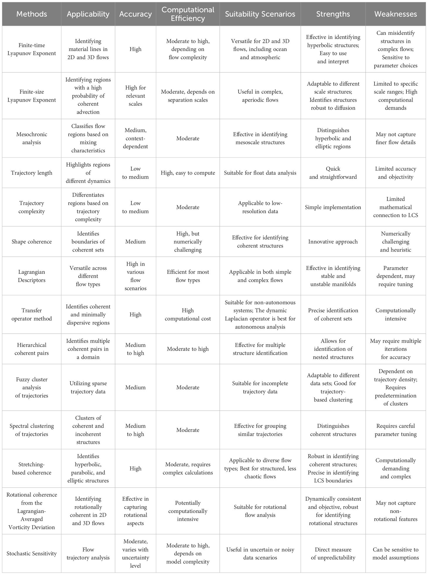
Table 1 Comprehensive comparison of various Lagrangian Coherent Structures detection methods (Allshouse and Peacock, 2015a; Hadjighasem et al., 2017; Badza et al., 2023).

According to the comparative analysis presented in Table 1, the FTLE method for detecting LCS demonstrates notable advantages in terms of accuracy and computational efficiency. Originating from Lorenz’s adaptation of the traditional Lyapunov exponent for basic atmospheric model analysis (Lorenz, 1963), the FTLE approach was further developed by Haller, who utilized the ridges of the FTLE field to define LCS boundaries between attracting and repelling particles within flows (Haller and Yuan, 2000; Haller, 2001b, 2002). The strength of the FTLE approach lies in its intuitive visualization capabilities, making it a user-friendly tool for interpreting complex fluid dynamics. This visualization ease, coupled with the method’s ability to yield reliable results even with significant errors in velocity field data, supports its widespread acceptance and application (Haller, 2002). Furthermore, as shown in Table 1, the versatility of the FTLE approach is evident in its applicability to both 2D and 3D flow analyses in various environments, including oceanic and atmospheric contexts. The FTLE method, therefore, has been extensively used, both independently and in conjunction with other techniques, to detect LCS to explain ocean fluid dynamics (d’Ovidio et al., 2004; Waugh et al., 2006; Waugh and Abraham, 2008; Pearson et al., 2023; Wang et al., 2024).

In this review, we distinctly shift our focus towards FTLE-based LCS and their applications in marine environments. This approach diverges from previous works, which predominantly concentrated on cataloging and evaluating a broad spectrum of LCS detection methods (Allshouse and Peacock, 2015a; Hadjighasem et al., 2017; Badza et al., 2023). Our objective is to bridge the theoretical developments in FTLE-based LCS with practical applications, particularly in understanding and managing marine ecosystems. This review, therefore, not only synthesizes the existing body of knowledge but also identifies emerging trends and potential areas for future research, thereby providing a fresh perspective on the application of LCS in marine science. Specifically, this review is organized as follows: Section 2 introduces the definitions, visualization, and interpretation of FTLE and LCS; Section 3 delves into their applications in understanding marine water mixing and transport mechanisms; Section 4 investigates the utilization of FTLE-based LCS in predicting the trajectories of specific floating entities, including pollutants and sea ice; Section 5 delves into FTLE-based LCS in identity marine species distribution and regions of conservation priority, and Section 6 discusses potential challenges and directions for future work.

2 Fundamentals of LCS and FTLE

LCS lines provide insights into surface transport dynamics, highlighting potential pathways for material transport by spreading or accumulating. Furthermore, LCS plays a significant role in shaping marine ecosystems and influencing the distribution of various species (Kai et al., 2009; Dargahi, 2022). As indicated in Table 1, FTLE (Haller and Yuan, 2000) and FSLE (Artale et al., 1997; Aurell et al., 1997) are prominent Lagrangian diagnostics. These methods are versatile and applicable to various data sources in marine science, including velocity fields from numerical modelling (d’Ovidio et al., 2004), HF radar observations (Shadden et al., 2009), and satellite altimetry (Beron-Vera et al., 2008). They are also effective when velocity field data from in-situ observations are unreliable (Nencioli et al., 2011), identifying regions with significant fluid strain and clarifying fluid flow dynamics (Samelson, 2013). Both methods, utilizing Lyapunov exponents, measure the rate of fluid particle separation. FTLE focuses on the separation rate of closely situated particles over finite times, providing local insights into flow chaos or predictability. Conversely, FSLE assesses the separation rate of particles initially at finite distances, offering perspectives on dispersion at larger spatial scales. Despite their utility, Karrasch and Haller (2013) demonstrated that FSLE and FTLE ridges do not generally coincide, casting doubts on FSLE’s reliability for LCS identification. Consequently, given its precise capabilities in local dynamics analysis, this review primarily concentrates on exploring and illustrating the various applications of FTLE.

2.1 Mathematical overview of FTLE

FTLE serves as a quantifier for the maximal rate of separation between trajectories over a finite time period, effectively interpreting LCS within various flow fields. The computation of FTLE begins by tracking the movements of tracer particles within a fluid, integrating their positions over a selected time interval. This process involves mapping the trajectory of a set of uniformly distributed tracer particles, which are initially located at position X at time t₀, to their positions after a duration T (Beron-Vera et al., 2008; Harrison and Glatzmaier, 2012). The mapping, described by the transformation ${\phi }_{t_0}^{t_0+T}(X)$, plays a critical role in understanding the dynamic behavior and shape changes of fluid parcels. To quantify the time-dependent deformation of fluid parcels over time, the Cauchy-Green deformation tensor, represented as $\Delta$, is employed. This tensor is computed using a finite-difference approximation of the derivative of the transformation ${\phi }_{t_0}^{t_0+T}(X)$ with respect to position $X$. This approximation is essential for estimating derivatives at discrete points and involves comparing the positions of neighboring particles at times $t_0$ and $t_0+T$. For 3D flows, this comparison includes the positions of six neighboring particles (see Figure 1) to approximate the sensitivity of the particle’s trajectory to its initial conditions. The formation of this tensor is represented in Equation 1, and the finite-difference approximation is shown in Equation 2.

Figure 1

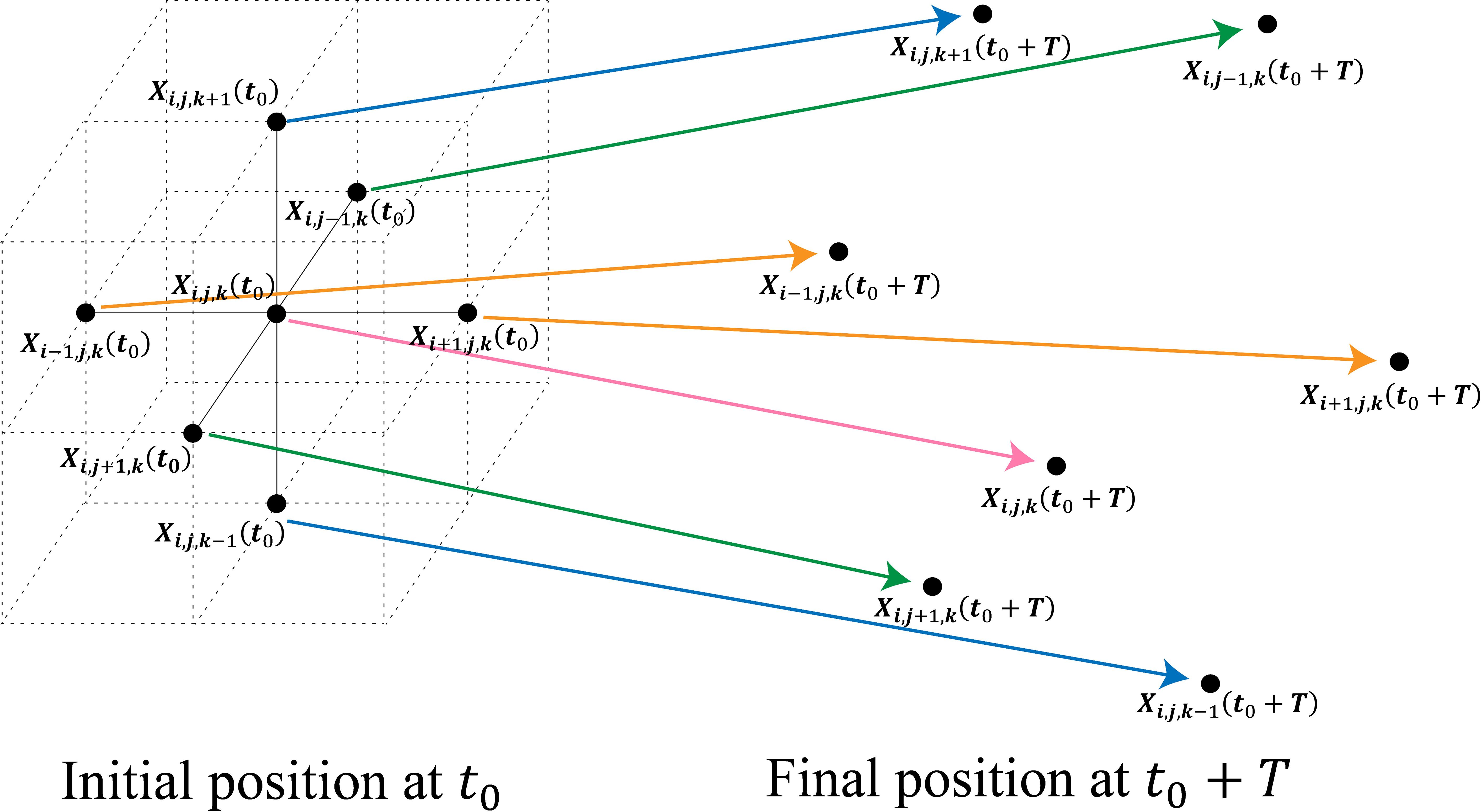
Figure 1 Schematic representation of particle grid evolution from time $t_0$ to $t_0+T$ for three-dimensional flows.

$\begin{array}{ll}\mathbf{\text{Δ}}={\frac{\mathit{\text{d}}{\phi }_{t_{\mathbf{0}}}^{t_{\mathbf{0}}+T}(\mathit{\text{X}})}{dX}}^{\text{'}}·\frac{d{\phi }_{t_{\mathbf{0}}}^{t_{\mathbf{0}}+T}(X)}{dX}& (1)\end{array}$

$\begin{array}{ll}\frac{d{\phi }_{t_{\mathbf{0}}}^{t_{\mathbf{0}}+T}(X)}{dX}\approx \left[\begin{array}{lll}\frac{x_{i+\mathbf{1},j,k}(t_{\mathbf{0}}+T)-x_{i-\mathbf{1},j,k}(t_{\mathbf{0}}+T)}{x_{i+\mathbf{1},j,k}(t_{\mathbf{0}})-x_{i-\mathbf{1},j,k}(t_{\mathbf{0}})}\hfill & \frac{x_{i,j+\mathbf{1},k}(t_{\mathbf{0}}+T)-x_{i,j-\mathbf{1},k}(t_{\mathbf{0}}+T)}{y_{i,j+\mathbf{1},k}(t_{\mathbf{0}})-y_{i,j-\mathbf{1},k}(t_{\mathbf{0}})}\hfill & \frac{x_{i,j,k+\mathbf{1}}(t_{\mathbf{0}}+T)-x_{i,j,k-\mathbf{1}}(t_{\mathbf{0}}+T)}{z_{i,j,k+\mathbf{1}}(t_{\mathbf{0}})-z_{i,j,k-\mathbf{1}}(t_{\mathbf{0}})}\hfill \\ \frac{y_{i+\mathbf{1},j,k}(t_{\mathbf{0}}+T)-y_{i-\mathbf{1},j,k}(t_{\mathbf{0}}+T)}{x_{i+\mathbf{1},j,k}(t_{\mathbf{0}})-x_{i-\mathbf{1},j,k}(t_{\mathbf{0}})}\hfill & \frac{y_{i,j+\mathbf{1},k}(t_{\mathbf{0}}+T)-y_{i,j-\mathbf{1},k}(t_{\mathbf{0}}+T)}{y_{i,j+\mathbf{1},k}(t_{\mathbf{0}})-y_{i,j-\mathbf{1},k}(t_{\mathbf{0}})}\hfill & \frac{y_{i,j,k+\mathbf{1}}(t_{\mathbf{0}}+T)-y_{i,j-\mathbf{1},k-\mathbf{1}}(t_{\mathbf{0}}+T)}{z_{i,j,k+\mathbf{1}}(t_{\mathbf{0}})-z_{i,j,k-\mathbf{1}}(t_{\mathbf{0}})}\hfill \\ \frac{z_{i+\mathbf{1},j,k}(t_{\mathbf{0}}+T)-z_{i-\mathbf{1},j,k}(t_{\mathbf{0}}+T)}{x_{i+\mathbf{1},j,k}(t_{\mathbf{0}})-x_{i-\mathbf{1},j,k}(t_{\mathbf{0}})}\hfill & \frac{z_{i,j+\mathbf{1},k}(t_{\mathbf{0}}+T)-z_{i,j-\mathbf{1},k}(t_{\mathbf{0}}+T)}{y_{i+\mathbf{1},j,k}(t_{\mathbf{0}})-y_{i,j-\mathbf{1},k}(t_{\mathbf{0}})}\hfill & \frac{z_{i,j,k+\mathbf{1}}(t_{\mathbf{0}}+T)-z_{i,j,k-\mathbf{1}}(t_{\mathbf{0}}+T)}{z_{i,j,k+\mathbf{1}}(t_{\mathbf{0}})-z_{i,j,k-\mathbf{1}}(t_{\mathbf{0}})}\hfill \end{array}\right]& (2)\end{array}$

where $(x_{i,j,k}, y_{i,j,k}, z_{i,j,k})$ denote the positions of particles in a 3D grid, with indices $i,j,k$ corresponding to their grid positions. For 2D flows, only the first 2 × 2 minor matrix of the tensor is relevant, considering the four nearest particles (Haller, 2015).

The FTLE, denoted as ${\sigma }_{t_0}^T (q)$, is then derived from the maximal eigenvalue, $\lambda max (\text{Δ})$, of this deformation tensor. It is calculated using the equation (Haller, 2001a):

$\begin{array}{ll}{\sigma }_{t_{\mathbf{0}}}^T (\mathit{\text{q}}) =\frac{1}{ \left|\mathit{\text{T}} \right|} ln \lambda max (\mathbf{\text{Δ}})& (3)\end{array}$

The parameter of T can assume both positive and negative values. Specifically, positive T values correspond to forward temporal separations, leading to the identification of repelling LCS. Conversely, negative T values are indicative of backward temporal separations, resulting in the detection of attracting LCS in a forward temporal framework (Haller, 2001a, 2002; Shadden et al., 2005). It is worth noting that the choice of interval time $T$, to accurately capturing meaningful flow structures and dynamics, depends on the characteristics of the fluid domain being studied and the specific objectives of the analysis. Primarily, the predominant time scales inherent to oceanic dynamics must be recognized, which often manifest as tidal, diurnal, or even seasonal variations (Huhn et al., 2012; Bakhoday-Paskyabi, 2020). The chosen FTLE interval ought to be matching with these time scales to ensure an accurate representation of oceanic motions. The overall research objective further defines the choices. Long-term FTLE evolutions require longer intervals (Bakhoday-Paskyabi, 2020; Paul and Sukhatme, 2020; Rypina et al., 2020; Dargahi, 2022), while transient phenomena require shorter spans (Castelle and Coco, 2013; Lee et al., 2013). Evaluating particle trajectory separations across various regions provides empirical insights into time interval selection (Shadden et al., 2009; Huhn et al., 2012). Meanwhile, analysis of the probability distribution function (PDF) of the FTLE field can highlight the dominant dynamics. Distinct peaks in the PDF suggest consistent behavior across the marine domain and indicate a suitable interval choice (Huhn et al., 2012). Sensitivity analyses, which involve calculating FTLE fields over various intervals, are useful in determining the point at which LCS remains consistent (Huhn et al., 2012).

2.2 Interpretation of FTLE and LCS

Upon computation, high FTLE values (FTLE ridges) serve as indicators, highlighting areas where particle trajectory separations are particularly pronounced. This distinction in the FTLE field provides a robust mechanism to detect regions of significant dynamical behavior, emphasizing areas of the flow domain where material lines experience accelerated stretching or filamentation (Allshouse and Peacock, 2015b). It’s also worth noting that areas distanced from FTLE ridges tend to exhibit minimal activity (Zhong et al., 2022).

A comprehensive analysis of the FTLE field requires both forward-time and backward-time FTLE computations. However, when analyzing both stretching and filamentation material lines, the overlapping of forward and backward FTLE fields can lead to interpretative challenges. Addressing this, d’Ovidio et al. (2004) integrated normalized forward and backward FTLE fields, thereby introducing the concept of hyperbolic FTLE fields as shown in Equation 4:

$\begin{array}{ll}FTL{E}^{\pm }=\frac{FTL{E}^{+}}{FTL{E}_{max}^{+}}-\frac{FTL{E}^{-}}{FTL{E}_{max}^{-}}& (4)\end{array}$

where ${\text{FTLE}}_{\text{max}}^{+}$ is the maximum of the forward FTLE and the ${\text{FTLE}}_{\text{max}}^{-}$ is the maximum of the backward FTLE. This innovative approach offers a finite-time generalization of the traditionally recognized concept of normally hyperbolic invariant manifolds in dynamic systems, providing clarity in the visualization and understanding of complex flow behaviors. Figure 2 interprets these concepts using a hyperbolic LCS representation. In Figure 2, the inflowing manifolds, shown by the red line, signify repelling LCS, while the outflowing manifolds, illustrated by the blue line, represent attracting LCS. The intersection of these two lines is the saddle point. Flow direction proximity to this hyperbolic pattern is indicated by the blank arrows in Figure 2. Inferring flow direction from LCS is important. As illustrated in Figure 2A, trajectories associated with the red line are drawn towards the saddle point, while those along with the blue line move away from it. Consequently, as the flow approaches the saddle point via the red line and subsequently departs along the blue line, the change of flow direction is observed. In the nearshore area, as shown in Figure 2B, when the hyperbolic LCS intersects with the shoreline, the shoreline assumes the role of a saddle point. Flow approaches the shoreline along the red line and away from the shoreline via the blue line (Huhn et al., 2012).

Figure 2

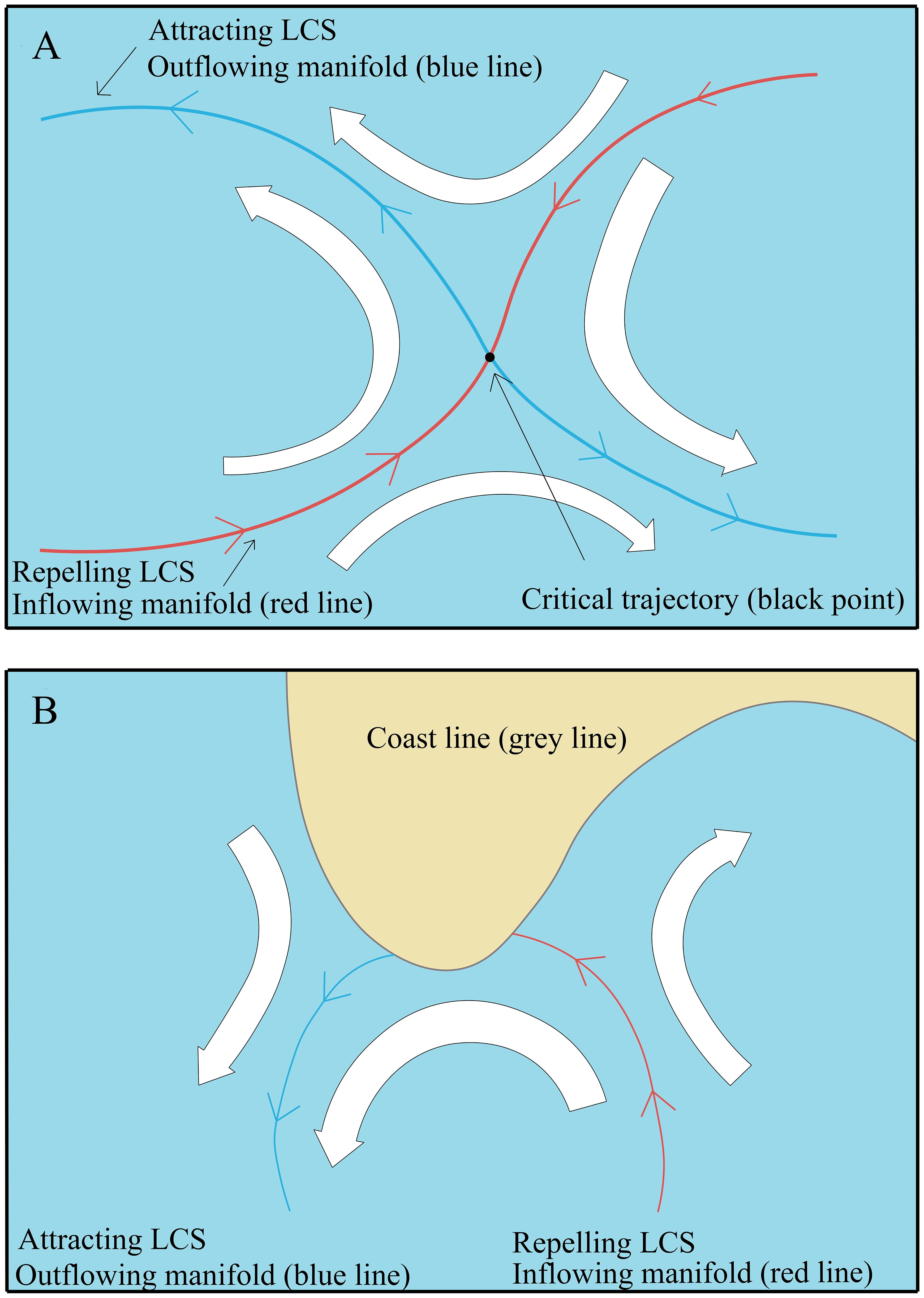
Figure 2 Hyperbolic Lagrangian Coherent Structures (LCS) in (A) open sea and (B) nearshore area. Red lines denote repelling LCS, while blue lines denote attracting LCS. The intersection of these lines constitutes the saddle point, with flow direction represented by the blank arrows.

The dynamics of stretching and filamentation in ocean fluids are inherently associated with the presence of LCS lines (Peacock and Dabiri, 2010; Peacock and Haller, 2013). Specifically, attracting LCS regions tend to draw fluid trajectories closer together, which can align and sometimes compress nearby material lines, making them more compact in the direction perpendicular to the stretching. Conversely, repelling LCS regions push trajectories outward, leading to the elongation and thinning of material lines as they are pulled apart (van Sebille et al., 2018). Consequently, these LCS lines act as transport barriers, inhibiting any flux across them (Shadden et al., 2005; Bettencourt et al., 2012; Huhn et al., 2012; Zhong et al., 2022). Wei et al. (2018) introduced two distinct particle sets on either side of LCS and monitored their paths over a span of 144 hours, it was documented that the majority of the simulated particles remained confined to their initial sides of LCS.

To better visualize and understand the behaviors of complex flow, various methods have been employed to extract LCS lines from FTLE fields (Garth et al., 2007; Sadlo and Peikert, 2007; Sadlo et al., 2011; Lipinski, 2012). A widespread approach involves setting a threshold to highlight regions where FTLE values exceed the specific value (Lipinski, 2012; Suara et al., 2020; Zhong et al., 2022). While the selection of an optimal threshold remains non-definitive, empirical investigations indicate that thresholds between 50 – 80% of the maximal FTLE value offer a reliable representation (Lipinski, 2012). Several research indicated that higher threshold values might narrow down the areas of significant activity without drastically altering the overall flow pattern (Rockwood et al., 2019; Giudici et al., 2021). The threshold selection is inherently subjective and should align with the analysis goals, the unique characteristics of the flow, and the level of detail and robustness required for identifying coherent structures.

3 Applications in marine water mixing and transport analysis

The mixing and transport of water masses are crucial dynamic processes in the ocean, which drive the circulation of seawater (Wunsch and Ferrari, 2004; de Lavergne et al., 2022), facilitating the systematic transfer of energy, heat, and matter across diverse marine regions. The understanding of these processes is important for accurately modeling and predicting ocean fluid dynamics (McDougall, 1988; Edwards and Marsh, 2005), clarifying interactions within marine ecosystems (Mann and Lazier, 2005), and realizing the ocean’s broader contributions to global biogeochemical cycles (Sonke et al., 2023). This section provides an overview of the application of FTLE-based LCS methods in understanding marine water mixing and transport mechanisms.

3.1 Characterization of fluid dynamics

Shear and confluence are fundamental components in interpreting complex dynamics and motions. Shear is characterized by velocity differentials between neighboring oceanic layers. Confluence, in contrast, refers to the stretching of water masses with differing attributes (Biron et al., 1993). Backward FTLE ridges (attracting LCS) were utilized to visualize shear and confluence regions (Haller, 2002; Gough et al., 2016). Gough et al. (2016) posited that areas with high FTLE values correspond with pronounced gradients in the velocity field, signaling regions of shear. Similarly, zones where LCS accumulate or are densely packed suggest areas of particle confluence. Through the temporal and spatial analysis of LCS, researchers are able to deduce the existence and dynamics of shear zones and confluence regions on the ocean’s surface (Gough et al., 2016).

Both shear and confluence can enhance or create strong horizontal gradients, leading to the formation of fronts (Owen, 1981; Gough et al., 2016). In oceanographic studies, fronts stand as a keystone of marine hydrodynamics, serving as the boundaries between different water masses (Mathur et al., 2019). These fronts play an important role in shaping the dynamics within marine systems and significantly influence global climatic interactions (Gough et al., 2016; Liu et al., 2018; Mathur et al., 2019). As an advanced analytical tool, FTLE and LCS were employed by Mathur et al. (2019) to explain the orientation of thermal fronts in the north Bay of Bengal from December 2015 to March 2016, as shown in Figure 3. These thermal fronts, presenting the boundary between seawater and freshwater from river runoff, were identified by locating regions where the magnitude of the spatial temperature gradient exceeds a specified threshold of 0.02°C/km (Mathur et al., 2019). The sea surface temperature (SST) field illustrated a prominent thermal front extending from around 14°N to 19°N at around 86°E, which was labelled as C-front (Figure 3B). This specific C-front feature exhibited similarity with the backward FTLE, as shown in Figure 3C. Furthermore, overlaying the extracted attracting LCS onto the SST field (Figure 3D) revealed a robust association between the location/orientation of thermal fronts and the attracting LCS in ocean surface currents. For instance, a concurrence between the attracting LCS and extensive C-front feature (about 700 km) was observed. Subsequent analyses revealed the persistence of this similarity between the attracting LCS and the thermal front over an extended duration of at least one month. Moreover, Mathur et al. (2019) introduced the angle $\alpha \in [0,\frac{\pi }{2}]$ for quantification purposes. The trajectory of thermal fronts is hypothesized to be orthogonal to the vector of ∇(SST), while the direction of the attracting LCS corresponds to the eigenvector associated with the maximum eigenvalue of the Cauchy-Green strain tensor. The outcomes, as shown in Supplementary Figure 1, highlighted that alignment between thermal fronts and proximal attracting LCS was particularly prominent in large-scale frontal features and any frontal feature if it located near a sufficiently robust attracting LCS. However, certain limitations, such as the reliance on 2D modeling data, potential errors in SST-gradient-corrections, and possible inaccuracies in satellite-based observations, should be acknowledged (Mathur et al., 2019).

Figure 3

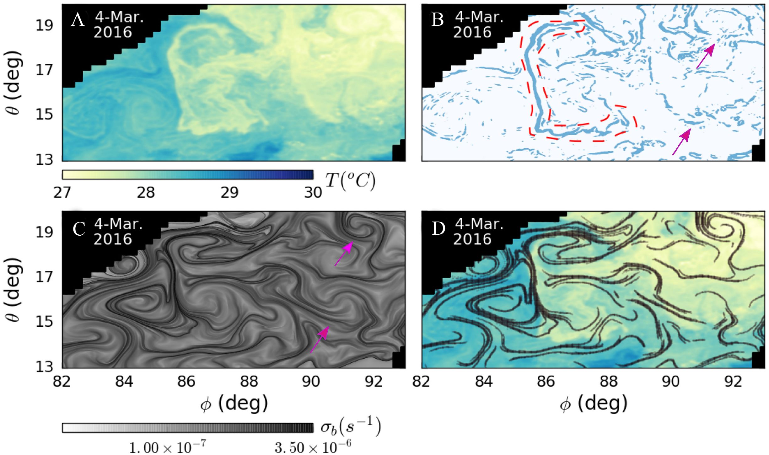
Figure 3 (A) Spatial distribution of sea surface temperature (SST) on 4 Mar. 2016, (B) Points (shown in blue) that satisfy |∇(SST)| > 0.02°C/km on 4 Mar. 2016, (C) the backward Finite-Time Lyapunov Exponent (FTLE) field (computed using T = 20 days) on 4 Mar. 2016, and (D) points (shown in black) that satisfy FTLE > 0.5 FTLE^max plotted on top of the SST distribution on 4 Mar. 2016. The red dashed line in (B) encompasses the C-front region. The pink arrows in (B, C) show other prominent features that are similar between the |∇(SST)| and backward FTLE fields. Adapted from Mathur et al. (2019) with permission.

Fronts can appear individually, in clusters, or conjunction with eddies throughout the oceans, especially within the surface layer (Owen, 1981). Eddies are localized circular current systems, which can be either cyclonic or anticyclonic (Chelton et al., 2011). Characterized by their vortical motion, these eddies play a pivotal role in trapping and transporting heat, nutrients, and contaminants within the marine environment (McWilliams, 2008). The application of FTLE-based LCS technique has become increasingly prevalent for examining the formation and dissipation of eddy, and the consequent implications on fluid mixing (Waugh et al., 2006; Waugh and Abraham, 2008; Prants et al., 2011, 2015; Gough et al., 2016; Liu et al., 2018; Paul and Sukhatme, 2020; Rypina et al., 2020; Zheng et al., 2020; Filippi et al., 2021). For example, Zheng et al. (2020) defined typical eddy activities and flow dynamics in the vicinity of the Luzon Strait using LCS framework. Employing a backward FTLE approach, LCS was extracted and subsequently compared against satellite-tracked drifter trajectories from corresponding dates. Notably, the observed LCS consistency with drifter patterns emphasizes its ability to define transport trajectories and determine boundaries within the investigated domain. Examination of FTLE fields revealed four major transport patterns proximal to the Luzon Strait, as shown in Figure 4. The first pattern presents a typical Kuroshio “leaking” trajectory, with LCS extending northwestward from the eastern precincts of Luzon Island into the South China Sea (SCS) (Figure 4A). The second pattern represents the northward “leaping” pattern of Kuroshio, the corresponding FTLE fields in Figure 4B display LCS along the Kuroshio trajectory, extending more distinctly northward compared to those shown in Figure 4A. The type of “looping” LCS near the Luzon Strait is clearly seen in the FTLE field in Figure 4C, which makes the water loop or excurse into the SCS and then turn clockwise back to the Pacific. The fourth type of pattern, called “outflowing” LCS, demonstrates the outflow of SCS waters into the Pacific, with the associated LCS emphasizing FTLE ridges extending northeastward from the western regions of Luzon Island to the eastern of Taiwan Island (Figure 4D). Additionally, these observed transport patterns show seasonal variations. Among them, the “leaping” pattern, predominant across seasons, peaked in spring, while “leaking” and “outflowing” patterns exhibited sensitivity to the monsoon reversals, prevalent in winter and summer, respectively. Interestingly, the “looping” pattern remained consistent across all seasons. On an annual scale, the leaping pattern’s frequency dominated, with notable deviations in 1998 and 2016 (Zheng et al., 2020).

Figure 4

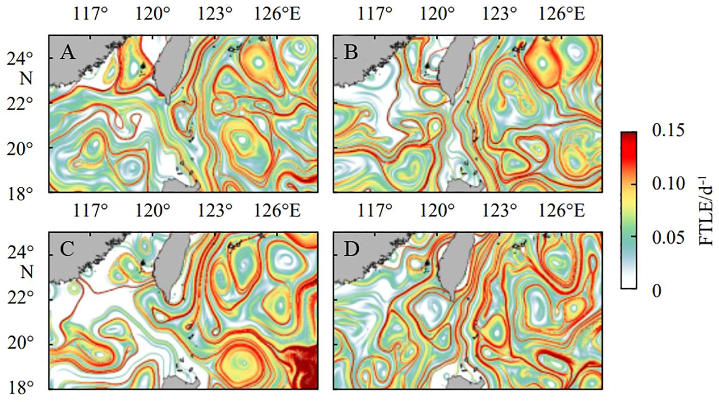
Figure 4 Typical snapshots of Finite-Time Lyapunov Exponent (FTLE) fields for (A) leaking Lagrangian Coherent Structures (LCS) type (March 8, 2003), (B) leaping LCS type (March 31, 2003), (C) looping LCS type (December 24, 2003), (D) outflowing LCS type (June 19, 2000). Adapted from Zheng et al. (2020) with permission.

In addition to surface eddies, the vertical eddies structure also plays an important role in enhancing the precision of simulations and predictions in oceanographic modeling. Prants et al. (2015) delved into the vertical structure of mesoscale anticyclonic eddies in the Japan/East Sea using an ocean circulation quasi-isopycnal layered model. By employing the FTLE fields, they highlighted the nonlinear stability of these eddies and their ability to reveal the complex pathways and barriers that determine transport and mixing processes at mesoscales and submesoscales. Their examination extended up to 250 meters deep, segmented into ten layers, with the 1^st, 3^rd, 5^th, and 9^th layers highlighted in Figure 5. A key observation was the presence of elliptic stagnation points at the eddy centers, characterized by zero velocity, particularly discernible in layers below the fourth. Through the FTLE field, the study detailed the eddy’s horizontal layer-by-layer structure, with “ridges” signifying areas of maximal particle filamentation. Such insights are crucial, suggesting that while particles on one side partake in vortex activities, those on the opposite move away from the eddy. Prants et al. (2015) also established that the simulated anticyclonic eddy underwent a seasonal transition. The structure at the subsurface during summer reached the surface by fall. This transitional behavior can be attributed to the variances in seasonal stratification, especially evident in the pycnocline. Moreover, their findings’ accuracy is validated through comparisons with a 1999 oceanographic survey (Talley et al., 2001, 2006), emphasizing its alignment with real-world observations (Prants et al., 2015).

Figure 5

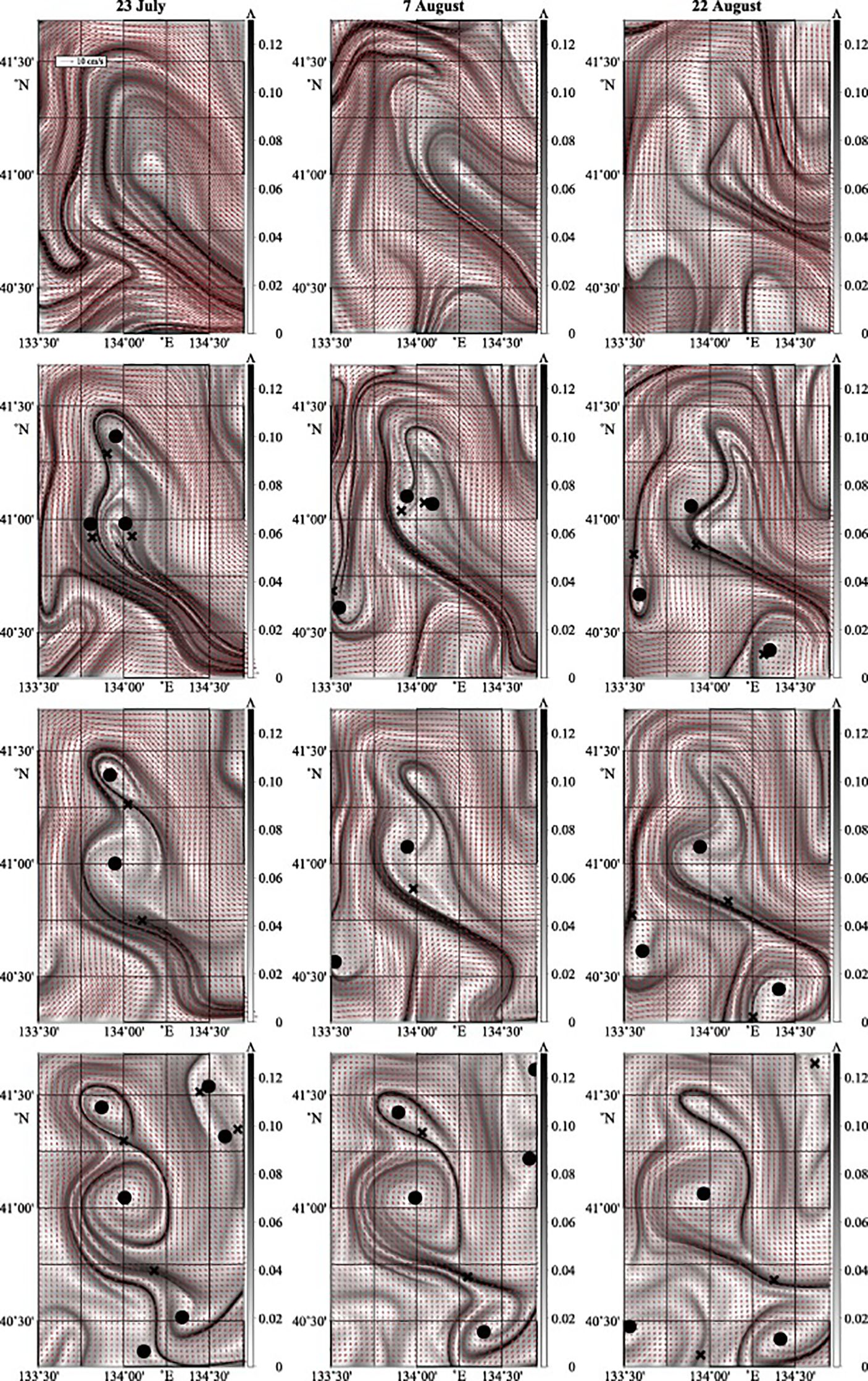
Figure 5 The vertical eddy structure was shown on 23 July, 7 August, and 22 August. The Finite-Time Lyapunov Exponent (FTLE) fields in the 1st, 3rd, 5th and 9th layers are shown from the top to the bottom, respectively. Elliptic and hyperbolic points are indicated by circles and crosses, respectively. Adapted from Prants et al. (2015) with permission.

To clarify the intensity and spatial distribution of turbulent eddy phenomena, the metric Eddy Kinetic Energy (EKE) was introduced to quantify the kinetic energy inherent to mesoscale eddies within fluidic systems, as given by the Equation 5 (Waugh et al., 2006):

$\begin{array}{ll}EKE=\frac{\mathbf{1}}{\mathbf{2}}(\langle u\text{'}{}^2\rangle +\langle v\text{'}{}^2\rangle )& (5)\end{array}$

where $u^{\prime }$ and $v^{\prime }$ represent temporal anomalies in the zonal and meridional velocities, respectively (i.e., deviations from their temporal mean), while angle brackets signify temporal averaging. Research has validated that FTLE effectively describes characteristics inherent to EKE on both localized (Waugh et al., 2006; Paul and Sukhatme, 2020) and global scales (Waugh and Abraham, 2008). For instance, Paul and Sukhatme (2020) created the FTLE maps across varying seasons, including February-March-April (FMA), June-July-August-September (JJAS), and October-November-December (OND). The patterns within these FTLE maps paralleled those of EKE for each season, with elevated EKE correlating with zones of strong stirring, underlining the efficacy of FTLE in revealing stirring intensities (Waugh et al., 2006; Waugh and Abraham, 2008; Paul and Sukhatme, 2020). Additionally, Waugh et al. (2006) introduced a strain rate to describe the deformation rate of fluid elements in flow, along with EKE for comparative analysis with FTLE fields. The strain rate is represented as shown in Equation 6 (Waugh et al., 2006):

$\begin{array}{ll}\gamma ={\left(\frac{\partial u}{\partial x}-\frac{\partial v}{\partial y}\right)}^{\mathbf{2}}+{\left(\frac{\partial v}{\partial x}-\frac{\partial u}{\partial y}\right)}^{\mathbf{2}}& (6)\end{array}$

where $(u, v)$ represents the total velocity field. The relationship between mean FTLE, strain rate, and EKE has been systematically quantified, as shown in Figure 6. In this depiction, individual markers denote individual grid points, while the boxes capture the mean values over 5° by 5° subregions. Notably, as indicated in Figures 6A, B, in regions characterized by higher strain rates, the corresponding FTLE values are consistently lower. The decrease in FTLE values in regions with higher strain rates is due to particles temporarily residing in areas of high strain. As the integration time increases, these particles move to areas with smaller strain rates. Consequently, the overall stretching rate (FTLE values) diminishes when compared to the initially higher strain rate (Waugh et al., 2006). On a global scale, Waugh and Abraham (2008) presented a comparative analysis of FTLE, strain rate, and EKE (Supplementary Figure 2 in supplemental materials). This comparison emphasizes the inherent relationships among these metrics, with their spatial distributions showcasing considerable overlap (Waugh and Abraham, 2008). The consistent representation of FTLE across various temporal scales, supported by EKE and strain rate analysis, highlights the importance of these metrics in interpreting marine dynamics.

Figure 6

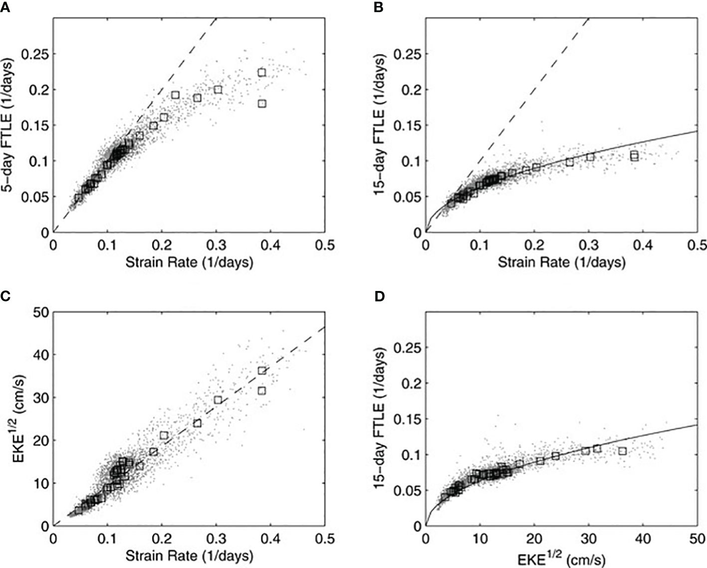
Figure 6 Comparative scatterplots illustrating (A) 5-day and (B) 15-day Finite-time Lyapunov Component (FTLE) versus strain rate (γ), (C) $EK{E}^{1/2}$ versus γ, and (D) 15-day FTLE versus $EK{E}^{1/2}$. Points represent individual grid locations, while boxes represent mean values across 5° x 5° subregions. (A) includes a 1:1 dashed reference line. Quadratic fits are shown as solid curves in (B, D), with a specific dashed line in (C) representing $EK{E}^{1/2}=L\gamma$, where L is 80 km. Adapted from Waugh et al. (2006), used with permission.

The FTLE has proven to be a critical tool in ocean fluid dynamics, particularly for revealing complex phenomena such as shear, confluence, oceanic front, and eddy. While traditionally used in a standalone capacity, FTLE’s effectiveness is further amplified when used in conjunction with metrics like EKE and strain rates in comparative analyses. This combined approach allows for a more comprehensive understanding of ocean fluid dynamics, offering a robust framework for exploring and interpreting the intricate dynamics of oceanic flows, thus significantly contributing to the advancement of marine research and modeling.

3.2 Influence of tide and wind forcing

Tidal forces and the resultant currents are influential in the generation of turbulence and mixing. These dynamics profoundly influence the transport of both dissolved and particulate substances, inducing periodic oscillations in the physical and chemical properties (Mao et al., 2004). Given the impact of tidal forces on the movement and patterns of water flow in the oceanic environment, it becomes vital to delve deeply into the influence of tides in these contexts (Wei et al., 2018; Suara et al., 2020; Filippi et al., 2021; Zhong et al., 2022). Wei et al. (2018) compared LCS during varied tidal phases within the Pearl River Estuary (PRE). Their comprehensive mapping, as shown in Figure 7, represented the hourly evolution of LCS over a tidal cycle. The evolution of LCS was periodic, aligning with the alternating ebb and flood tidal currents (Figures 7A-O). This periodicity approximated a duration of 12.5 hours, which is consistent with the predominant tidal phase in the PRE. During ebb tide, an obvious repelling LCS was formed in the high dynamic area and separated the mid-estuary into two parts, as highlighted by a blue quadrangle in Figure 7B. This LCS line formed after high tide, persisting for 6 to 7 hours, dissipating just prior to low tide (Figures 7J-N) (Wei et al., 2018). Similarly, Filippi et al. (2021) employed FTLE to investigate transport mechanisms during different tidal phases within Scott Reef. They recommended that the repelling/attracting LCS resulted from the filamentation/stretching. Their findings illustrated that tidal forces had a significant influence on LCS formation within the studied region. Specifically, the stretching was strongest during the high tide phase at 6:00 UTC. This stretching then undergoes a systematic decrease throughout the ebb period. Furthermore, they observed minimal filamentation/stretching at the low tide at 12:00 UTC, followed by an increase in filamentation during the flood period.

Figure 7

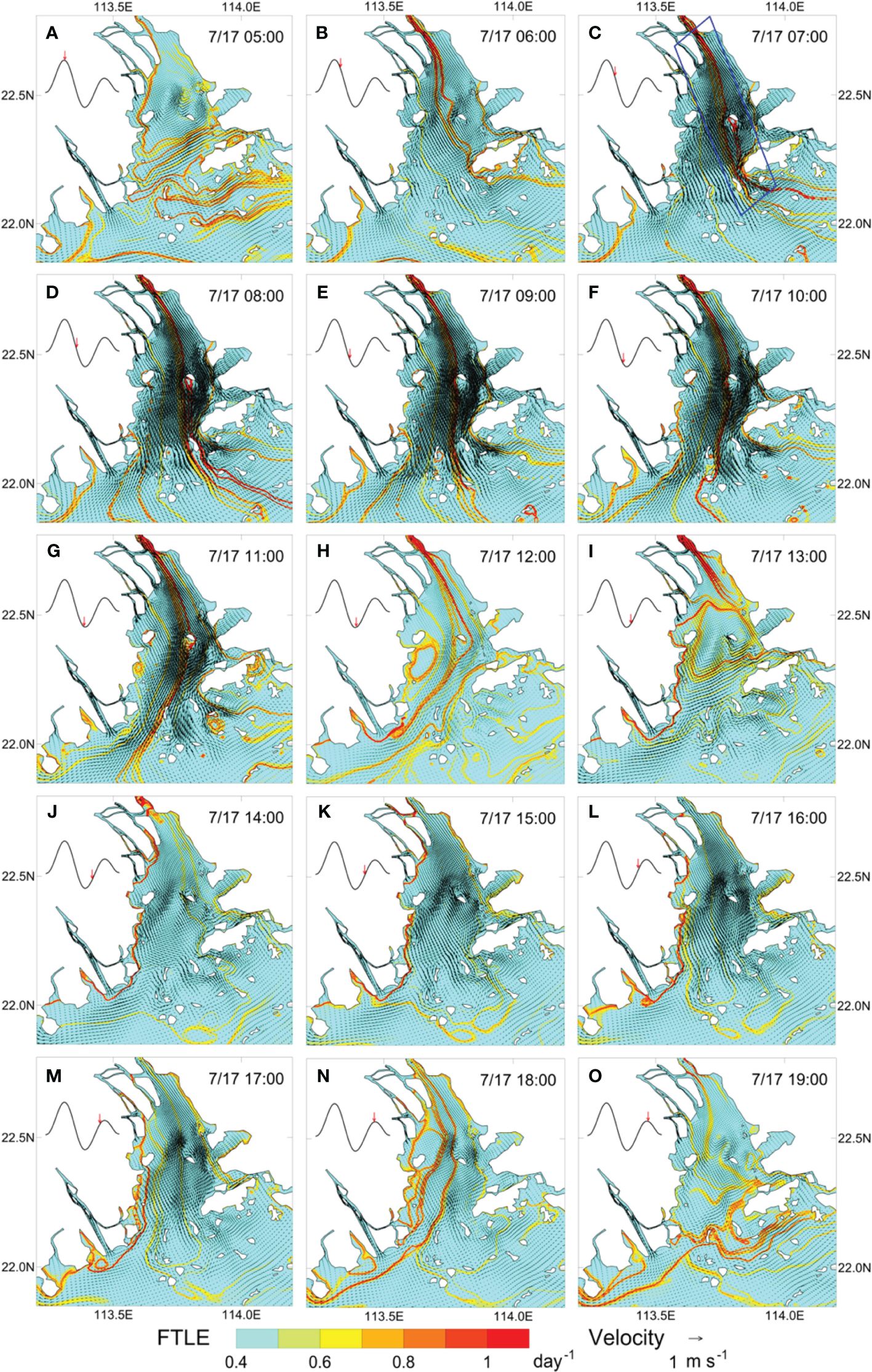
Figure 7 Repelling Lagrangian Coherent Structures (LCS) at different tidal phases on 17 July 1999 in PRE. (A–H): ebb tide. (I–O): flood tide. Adapted from Wei et al. (2018) with permission.

Wind-driven processes significantly influence oceanic surface transport through the additional drag force they exert, which propels the movement of floating materials directly at the ocean’s surface. FTLE and LCS have been at the forefront of a new perspective on understanding the wind’s role in oceanic material transport (Huhn et al., 2012; Gough et al., 2016; Allshouse et al., 2017; Wei et al., 2018; Suara et al., 2020). For instance, Huhn et al. (2012) investigated the influence of wind on ocean surface transport in Ria de Vigo by extracting the repelling and attracting LCS under southern and northern wind conditions, respectively, as shown in Figure 8. Under southern wind conditions (Figure 8A), the repelling LCS separates the flow at the Cies Islands (L1) and Cape “Cabo Home” (L2), facilitating the transport of water in-between L1 and coast into the Ria de Vigo at the south, and other water bodies leave the estuary through the north mouth. Moreover, the attracting LCS (L3) connected to the north of Cies Island suggests that this outflow remains coastal, progressing northward into the Ria de Pontevedra. Conversely, during northern wind conditions (Figure 8B), the flow largely inverts. An attracting LCS (L4) restricts surface water entry into the inner estuary from the north. Although there exists some variability in LCS during different wind directions, they consistently represent model flow patterns under similar meteorological conditions. Consequently, wind is recognized as an indispensable parameter in utilizing LCS methodology to assess marine water transport dynamics. Such a premise is corroborated by the findings of Allshouse et al. (2017) and Suara et al. (2020).

Figure 8

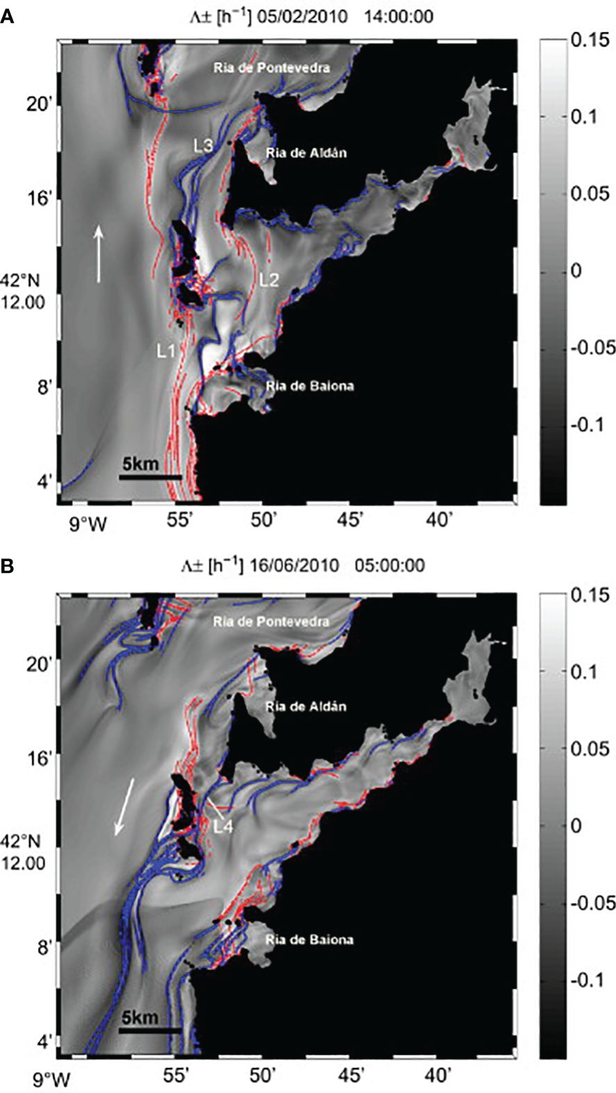
Figure 8 Lagrangian Coherent Structures (LCS) (red lines represent the repelling LCS, while blue lines represent the attracting LCS) in the Ria de Vigo for two typical meteorological situations: (A) south wind in winter and (B) north wind in summer. White arrows denote the approximate direction of the mean flow on the shelf. Adapted from Huhn et al. (2012) with permission.

Gough et al. (2016) also investigated the influence of wind forcing on the formation of LCS by comparing LCS identified through High-Frequency (HF) radar-derived velocities and patterns observed in satellite SST imagery. They found that during periods of light winds, LCS appeared to be influenced by circulation beneath the surface mixed layer. However, in conditions of moderate upwelling winds, there were noticeable shifts between LCS and SST fields, suggesting a decoupling of the surface mixed layer from the underlying water circulation. This decoupling became even more pronounced during strong winds, leading to a complete separation of the surface mixed layer from the circulation below, indicating that the surface currents captured by HF radar predominantly aligned with the wind-induced dynamics rather than the patterns in the SST imagery. Such findings underscore the complexity of interactions between surface and subsurface oceanic layers, and the significant role of wind conditions in these dynamics. The study highlights the value of LCS in understanding water movement patterns, providing insights that are not readily obtainable from SST images alone (Gough et al., 2016).

Tidal forces and wind-driven processes significantly shape ocean fluid dynamics, influencing the mixing and the transport of substances. Ser-Giacomi et al. (2015) introduced a novel method to study geophysical fluid transport, integrating the FTLE method with network theory. This approach establishes a direct correlation between the node degree in a flow network and the local fluid stretching, traditionally quantified by FTLE. The method uniquely applies FTLE to inform flow network construction, linking the nodes’ in-degree and out-degree to backward and forward FTLE values, respectively. This reflects the dispersion and mixing potentials of fluid parcels. The combination of FTLE and network theory offers a comprehensive perspective on fluid transport, merging local dynamic quantification with a structural overview of system-wide connectivity and pathways. This innovative fusion enhances the understanding of fluid motion, identifying key dispersion regions and major mixing zones in the fluid transport system (Ser-Giacomi et al., 2015).

Tidal forces and wind-driven processes are integral in shaping ocean fluid dynamics, notably affecting substance mixing and transport. The impact of tidal forces on water flow patterns is marked by periodic oscillations. Understanding these tidal influences is vital, as demonstrated through the use of FTLE to visualize changes in tidal phases and their corresponding effects on water movement. Similarly, wind plays a pivotal role in oceanic surface transport, altering the movement of floating materials through additional drag forces. The application of FTLE provides insights into how wind affects oceanic material transport. These approaches have revealed the complex interactions between surface and subsurface oceanic layers under varying wind conditions, highlighting the critical role of wind in influencing marine dynamics. Overall, the understanding of both tidal and wind forces, facilitated by FTLE-based LCS, is essential in comprehensively interpreting ocean fluid dynamics.

4 Applications in coastal pollution and sea ice dynamics

Tracking and forecasting the pathways of floating pollutants, recoverable debris, and sea ice are crucial aspects of oceanographic research. The FTLE and LCS methods provide detailed insights into the patterns of filamentation and stretching through strong temporal correlations. In previous work, these techniques have been successfully employed in interpreting the distribution and fate of pollutants, suspended sediments, and other floating entities on the ocean’s surface (Lekien et al., 2005; Szanyi et al., 2016; Ivić et al., 2017; Wei et al., 2018; Bakhoday-Paskyabi, 2020; Suara et al., 2020; Giudici et al., 2021; Zhong et al., 2022). This section offers a review of research efforts concerning the transit patterns of specific floating materials on the ocean surface. We begin by summarizing studies centered on analyzing pollutant dispersion in coastal environments, followed by the simulations focused on particular items like sea ice, taking into account their unique properties.

4.1 Examination of coastal pollutant dispersal

The applications of FTLE-based LCS analysis in coastal zones have provided profound insights (Lekien et al., 2005; Bakhoday-Paskyabi, 2020; Suara et al., 2020). For example, Bakhoday-Paskyabi (2020) employed FTLE-based LCS method to evaluate barriers impeding the spread of ocean contaminants and the distribution of marine populations in the Lofoten area of the Norwegian Sea. Their observations revealed that LCS lines within the region between 67° – 70° N and 10° – 15° E acted as a barrier to the dispersion of pollutants, dynamically separating the coastal and open-ocean water masses (Bakhoday-Paskyabi, 2020). Further delving into the seasonal variability of LCS (Figure 9), they suggested that the seasonal variability of surface currents, freshwater influx from riverine sources and precipitation, and water depth, are the key factors for LCS formation (Bakhoday-Paskyabi, 2020). Beyond the 70°N latitude, transport barriers during the winter months appeared to direct pollutants toward the Barents Sea (Bakhoday-Paskyabi, 2020). However, this effect is reduced during summer, and shelf waters can easily move into deeper Arctic waters (Bakhoday-Paskyabi, 2020). The seasonal variation of LCS was also studied by Giudici et al. (2021). They identified a strong correlation of LCS with specific wind patterns in different seasons, which informs the prediction of pollutant trajectory (Giudici et al., 2021).

Figure 9

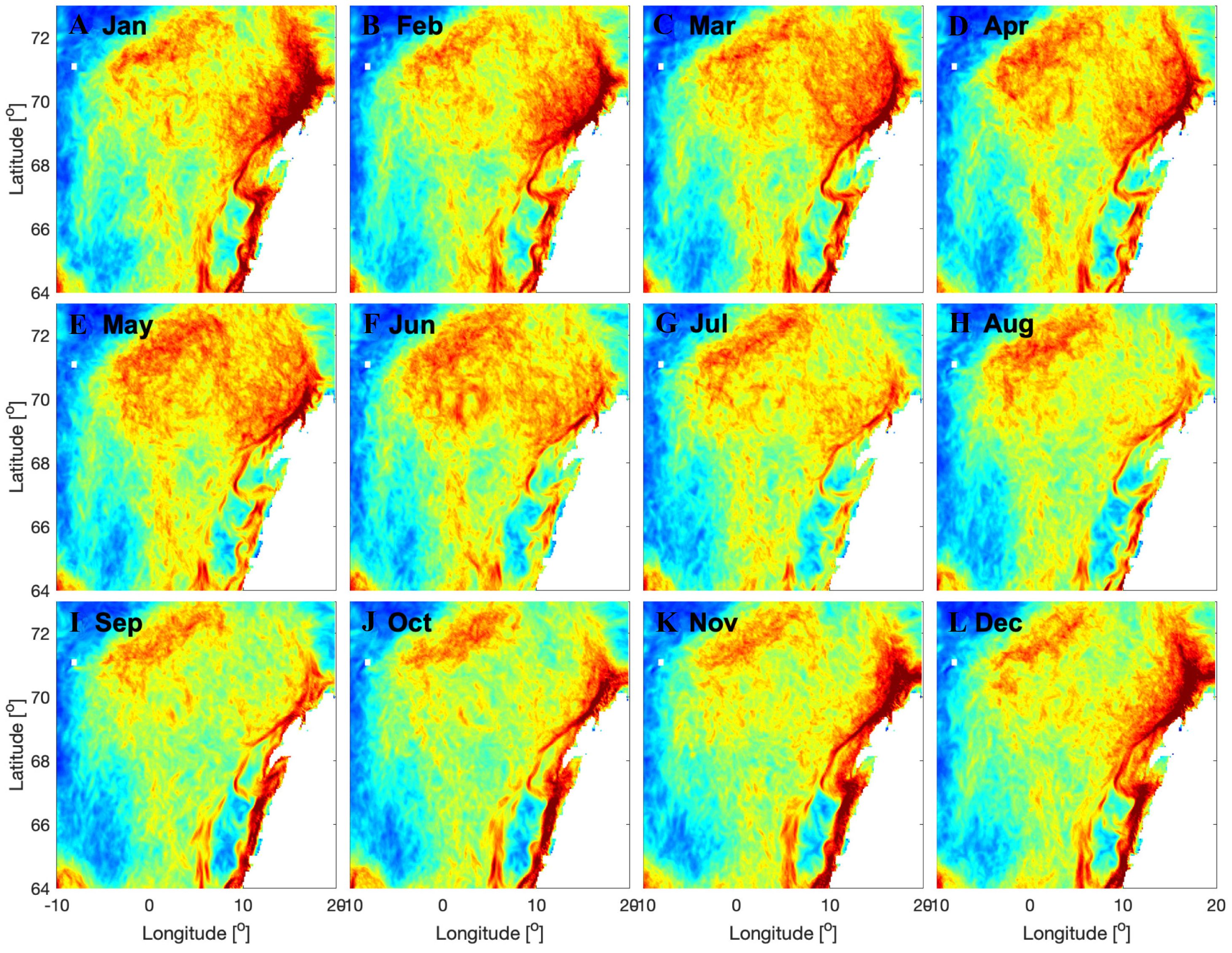
Figure 9 LCS approximated from the ridges of backward FTLE fields by time averaging of daily FTLE fields over 2007–2017 for T=7 days. (A–L) illustrate the FTLE fields for each month throughout the years. BS denotes the Barents Sea and LT denotes Lofoten. Adapted from Bakhoday-Paskyabi (2020).

The industrial infrastructures are commonly located in coastal regions, and the effluents discharged from factories represent a primary source of marine pollution. Therefore, Lekien et al. (2005) employed LCS to create a pollutant release strategy aimed at minimizing the impact of industrial effluents on the coastal environment. They utilized the VHF-radar-derived surface current data from the Florida coast to compute the forward FTLE fields, which identified a sequence of repelling LCS lines. These LCS originated from the coast and extended in a southward direction, as illustrated in Figure 10. LCS acts as a material barrier separating the southwest and northeast regions. Therefore, particles originated in the northeast of this barrier (white parcel) are rapidly spread within hours. In contrast, particles originating southeast of the barrier (black parcel) tend to undergo multiple re-circulation events near the Florida coast prior to their eventual integration with the currents. Notably, the position of LCS exhibits temporal variations. As such, industrial and sewage facilities should not release effluents when LCS is situated to the north of their discharge pipelines. According to the temporal variation of LCS, researchers proposed an optimal effluent release timetable, which can diminish the environmental impact of pollutants in the coastal zone by a factor of three, compared to a consistent temporal release (Lekien et al., 2005).

Figure 10

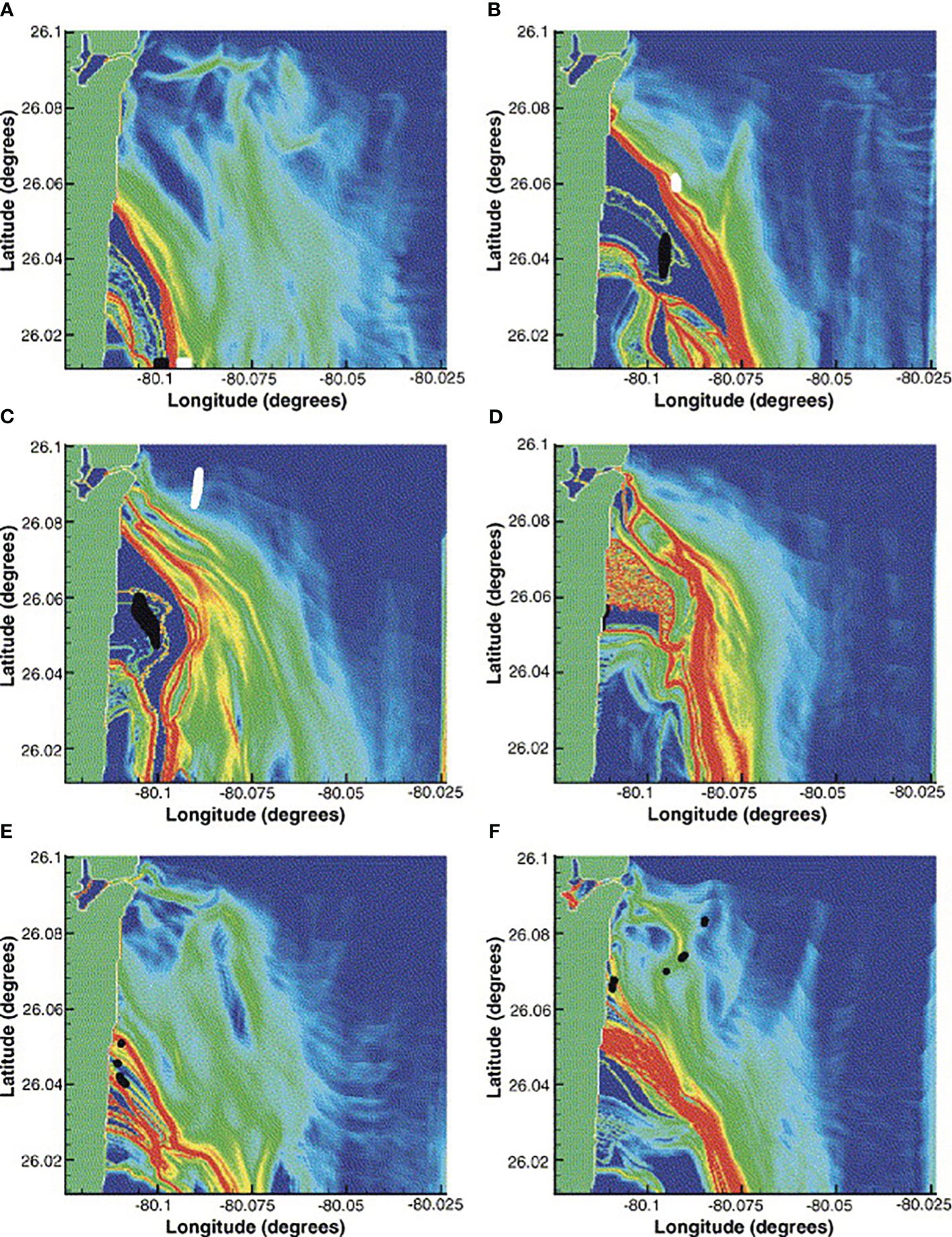
Figure 10 Forward Finite-time Lyapunov Component (FTLE) fields along the coast of Florida on (A) July 10, 1999 09:45 GMT, (B) July 10 13:45 GMT, (C) July 10 16:45 GMT, (D) July 10 23:45 GMT, (E) July 11 11:45 GMT and (F) July 11 20:45 GMT. Adapted from Lekien et al. (2005) with permission.

Marine debris contamination is emerging as a critical issue in the area of marine pollution. A thorough understanding and predictive ability regarding the sources, pathways, and exchange mechanisms of this debris are essential to address the issue effectively. Studies have identified FTLE-based LCS as a powerful tools to handle these challenges (Kim et al., 2012; Ourmieres et al., 2018; Suara et al., 2020; Ghosh et al., 2021). As a case in point, Suara et al. (2020) utilized the FTLE method to predict the fate of marine debris in the tidal embayment of Moreton Bay (MB). The extraction of LCS from the FTLE was achieved using a threshold, such that only FTLE values exceeding 50% of the maximum value were considered as LCS. Subsequent findings revealed that most LCS are attached to islands within MB, as illustrated in Figure 11. These LCS findings are consistent with the documented debris source data (Suara et al., 2020). Weak LCS lines were observed in Deception Bay (DB), coincidently quite much marine debris (32%) was observed in DB. However, only 16% and 7% of marine debris were detected in Redcliffe Headland (RCH) and Bramble Bay (BB) where had strong LCS lines. These suggested that the transport of marine debris cannot cross LCS lines (Suara et al., 2020). They also suggested that the presence of islands and headlands within the embayment critically influences LCS structure, subsequently affecting the transport and dispersion of debris. This observation was consistent with subsequent studies where LCS was employed to assess the persistency of debris accumulation in MB (Ghosh et al., 2021). By measuring LCS during the cumulative duration of time (14 days), most detected debris accumulation zones were identified as proximal to the islands and headlands of MB (Ghosh et al., 2021). Furthermore, both Suara et al. (2020) and Ghosh et al. (2021) evaluated the impact of tidal phases and wind dynamics on LCS formations in MB, noting the variability in structure and saddle point locations across different tidal phases. Their observations also highlighted wind as a factor amplifying the contraction and expansion rates near barriers, decreasing mixing intensities, and altering particle transport direction (Suara et al., 2020; Ghosh et al., 2021).

Figure 11

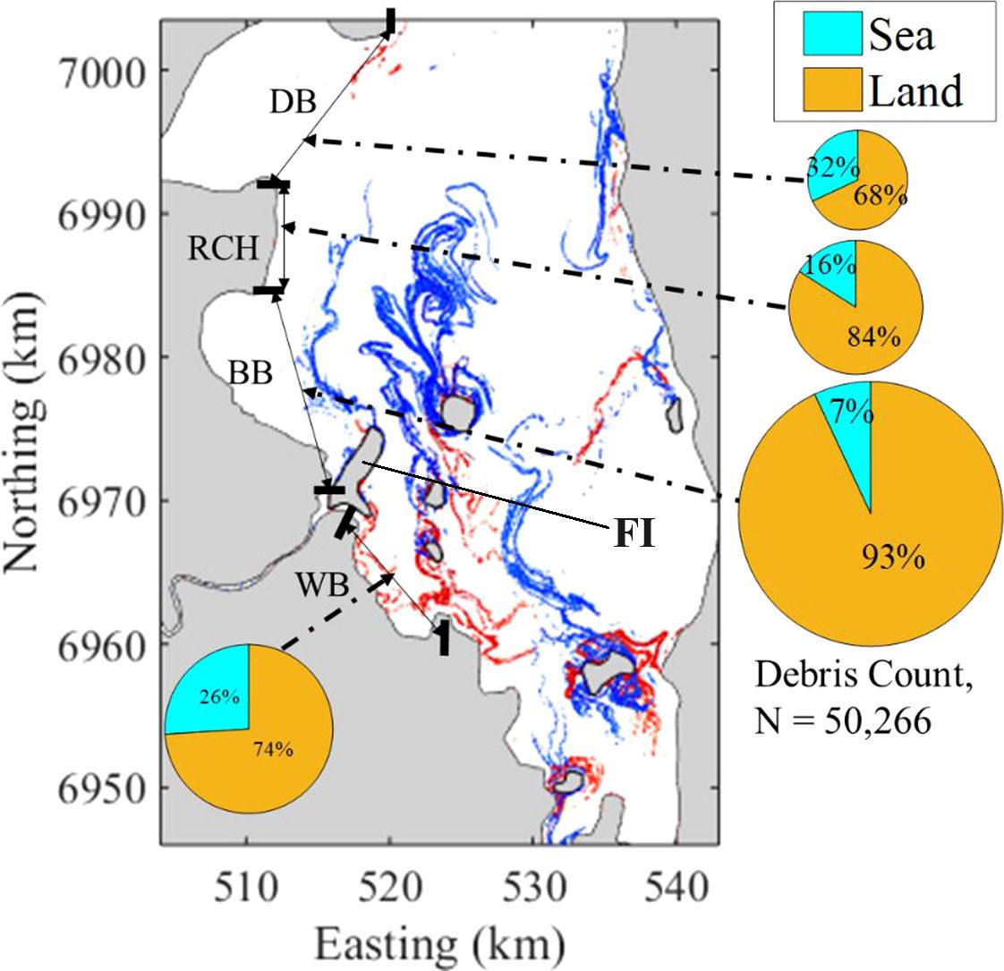
Figure 11 Lagrangian Coherent Structures (LCS) (Red lines represent the repelling LCS, while blue lines represent the attracting LCS) in Moreton Bay and the distribution of marine debris collected from the shoreline during 2011 and 2018 (DB, Deception Bay; RCH, Redcliffe Headland; BB, Bramble Bay; WB, Waterloo Bay; FI, Fisherman Island). Adapted from Suara et al. (2020) with permission.

The increase in petroleum product consumption and transportation has raised concerns about potential oil spills. Consequently, recent studies have employed the FTLE and LCS methods to predict oil spill trajectories (Ivić et al., 2017; Gough et al., 2019; Zhong et al., 2022). For instance, Zhong et al. (2022) utilized forward and backward FTLE fields to evaluate the influence of tidal dispersion on oil spill trajectory. By normalizing and combining the backward and forward FTLE fields with Equation 3 in Section 2.2, they generated the hyperbolic FTLE field. This field was compared with the real situation of the M/V Marathassa oil spill on April 8, 2015 (Butle, 2015). Given the spill started at 14:00 during a mid-ebb phase of the spring tide (Zhong et al., 2018), the corresponding FTLE field was compared with a recorded situational map from the City of Vancouver (Stormont, 2015). This comparative analysis, illustrated in Figure 12, robustly represented the actual dispersion patterns of the M/V Marathassa oil spill. For instance, Figure 12A demonstrates repelling LCS lines (in red) linking the Outer Harbour’s center to its eastern end, correlating with observed oil deposits at English Bay Beach and Siwash Rock (Figure 12B). Additionally, the migration of oil from the Outer Harbour’s north coast to the Inner Harbour via First Narrows during April 9 – 10, 2015, is corroborated by attracting LCS lines (in blue). Notably, no oil was observed on the southern shoreline of the Outer Harbour, aligning with the east-west orientation of repelling LCS lines preventing southern transportation. Essentially, these FTLE insights afford a comprehensive understanding of the M/V Marathassa spill dynamics. Zhong et al. (2022) also integrated a stochastic approach via the Oil Spill Contingency and Response (OSCAR) model to determine contamination probabilities at six potential spill locations in Burrard Inlet. This model’s outcomes fit with the FTLE-derived interpretations, underscoring FTLE’s effectiveness as a powerful tool for predicting oil spill trajectories and supporting spill response strategies (Zhong et al., 2022).

Figure 12

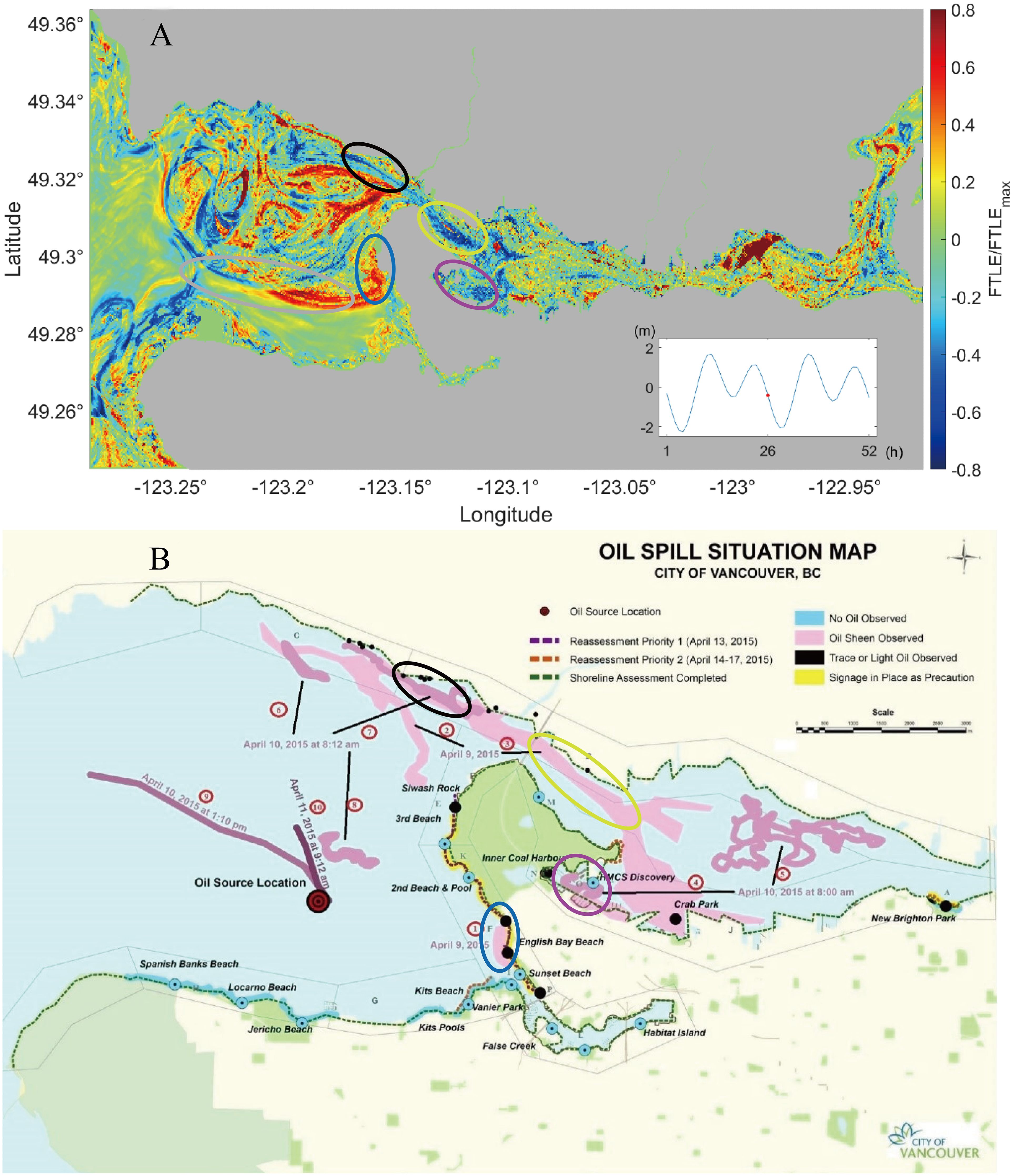
Figure 12 Comparison of (A) normalized hyperbolic Finite-Time Lyapunov Exponent (FTLE) fields during a mid-ebb phase of the spring tide for Burrard inlet and (B) the M/V Marathassa oil spill situation map. Adapted from Stormont (2015) and Zhong et al. (2022) with permission. The red line represents the repelling Lagrangian Coherent Structures (LCS), while the blue line represents the attracting LCS.

Overall, the application of FTLE-based LCS analysis in coastal regions has significantly advanced our understanding of pollutant dispersion. Researchers have been able to identify barriers that block the spread of contaminants and influence the distribution of pollutants. Seasonal variability in LCS, influenced by factors such as surface currents, freshwater influx, and water depth, further affects pollutant dispersion patterns. In addition, the role of wind and tidal forces in shaping LCS structures highlights their impact on debris transport and accumulation in coastal embayment. These insights are crucial for understanding pollutant trajectories and developing effective strategies for environmental protection. The integration of LCS with other models, such as oil spill contingency and response simulations, demonstrates the potential of these tools in predicting and managing marine pollution incidents, making them indispensable in marine environmental research.

4.2 Exploration of sea ice dynamics

Sea ice serves as a critical regulator in the energy exchange among the atmosphere, cryosphere, and ocean. Documented decreases in sea ice coverage, coupled with a rise in younger/thinner ice, underscore a concerning trend (Rothrock et al., 1999; Rignot et al., 2008; Landy et al., 2022). The younger/thinner ice is more sensitive to processes of deformation and breakage, which could subsequently change the atmospheric circulation patterns (Moore et al., 2018) and midlatitude weather (Siew et al., 2020). This highlights the urgency of precise monitoring of sea ice dynamics to comprehend the nuances of sea ice deformation, fracturing, and refreezing, as well as to assess their broader implications for global climate and maritime infrastructure.

Several studies have employed FTLE methods to investigate the dynamic of sea ice (Szanyi et al., 2016; Kumar et al., 2018). For instance, Szanyi et al. (2016) utilized the FTLE field to explore the dynamical shifts in the Arctic sea ice from November to April during 2006 to 2014 (Szanyi et al., 2016). Their analysis showcases three prominent regions of strong deformation, evident through clear LCS lines, which were consistent with the multi-year ice coverage data. Moreover, they introduced the Lagrangian Averaged Divergence (LAD) to distinguish the relative contributions of filamentation, shear and hyperbolic structures. The filamentation-induced ice deformation was observed in the Beaufort Sea, while shear predominantly influenced the central Arctic. FTLE ridges in the central Arctic exhibited influence from both shear and filamentation (Szanyi et al., 2016). Further comparison of FTLE results with multi-year ice (MYI) presented a noticeable correlation between high FTLE values and decreased MYI coverage (Szanyi et al., 2016).

5 Applications in marine ecosystems investigation

Marine ecosystems, characterized by complex ecological interaction and vast biodiversity, play a pivotal role in maintaining global ecological balance. Given the increasing pressure on marine ecosystems, including overfishing, contaminant influx, and climate-induced phenomena such as oceanic acidification and thermal elevation, the significance of using advanced analytical tools in marine research is paramount. FTLE-based LCS has been found to be effective in marine ecosystems research (Olascoaga et al., 2008; Winkler et al., 2008; St-Onge-Drouin et al., 2014; Maps et al., 2015; Dargahi, 2022). Utilizing these tools refines understanding of species distribution dynamics (St-Onge-Drouin et al., 2014; Wu et al., 2017; Rypina et al., 2020), algae bloom (Olascoaga et al., 2008; Dargahi, 2022), marine animal behavior (Soori and Arshad, 2009; Katija et al., 2011; Maps et al., 2015; Dawoodian and Sau, 2021; Dawoodian et al., 2021), and regions of conservation priority (Scales et al., 2018).

A comprehensive study was conducted by St-Onge-Drouin et al. (2014) to investigate the distribution of two genetically distinct Eurytemora affinis in the middle St. Lawrence Estuary using FTLE-based LCS. As shown in Figure 13, LCS line splits the area within the blue rectangle into two regions, corresponding to the habitats for the genetically distinct Eurytemora affinis. Subsequent particle tracking simulations further proved that particles cannot cross LCS line. This observed separation highlights the critical role of hydrodynamic mechanisms in maintaining the isolation between the two clades of the Eurytemora affinis species (St-Onge-Drouin et al., 2014).

Figure 13

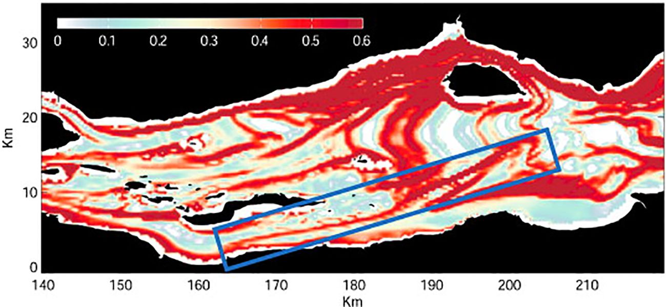
Figure 13 Finite-time Lyapunov Exponent (FTLE) fields in the St. Lawrence Estuary. Adapted from St-Onge-Drouin et al. (2014) with permission.

The distribution of certain species, such as kelp forest, has been identified to have the potential to alter hydrodynamic processes. A particular exploration of this phenomenon was carried out by Wu et al. (2017), which investigated how the presence of kelp forest modified the hydrodynamic processes within the Hecate Strait through FTLE-based LCS analysis. They observed significant differences in the spatial structure and magnitudes of the FTLE between the scenarios with and without the kelp effect. Specifically, in the absence of the kelp effect, ridges of FTLE predominantly surround islands, closely aligning with pronounced velocity shears along coastlines. Conversely, with the kelp effect, the spatial pattern of FTLE was predominantly determined by the extent of kelp beds. The ridges were located mainly along the edges of kelp forests due to velocity shear, driven by the enhanced velocity along kelp bed edges. This altered hydrodynamic pattern directed the tracers to predominantly move along the kelp forest edge, suggesting that the kelp beds serve as barriers, preventing outside tracers entering the interiors of the kelp forest. Delving into the FTLE magnitude in dense kelp regions, it was illustrated that while the kelp density diminishes dispersion rates within its interiors, it concurrently increases the dispersion rate along its edges. This comprehensive study underscores the essential role of species distribution in shaping hydrodynamic processes in marine ecosystems (Wu et al., 2017).

Algae are important in sustaining the biosphere by offering energy and nutrients. Nevertheless, some species are known for their potential harmful effects on a variety of organisms (Hallegraeff, 1993; Landsberg, 2002). Several theories have been proposed to explain the development of harmful algal blooms (HABs). However, a significant challenge in verifying these theories stems from the typically undetected early stages of HABs (Olascoaga et al., 2008). To address this, Olascoaga et al. (2008) utilized FTLE and LCS methods to determine the growing locations of HABs. Specifically, the study backtracked the 2004 HABs incident caused by the toxic dinoflagellate Karenia brevis on the West Florida Shelf through FTLE. The study presented the probable developing pathways and movement of HABs, guided by the material fluid barriers defined by LCS (Olascoaga et al., 2008). They also explored the potential factors contributing to this particular HABs’ incident combining a simplified nutrient-phytoplankton population dynamic model. The analysis identifies two major nearshore nutrient sources, closely aligned with LCS, indicating a substantial probability that land runoff plays a crucial role in the development of HABs (Olascoaga et al., 2008). Dargahi (2022) extended research to deeper oceanic depths to explore the dynamics of algal bloom development in the Baltic Sea. By computing LCS derived from FTLE fields across 34 Z-layers, covering a depth of 143.5 m, the patterns of algal bloom exhibited an evident correlation with LCS in terms of patterns, duration, and dispersion tendencies. LCS functioned as channels, facilitating the transport of mixed waters, nutrients, and oxygen from the sea surface down to the ocean floor, leading to increased eutrophication and the extensive growth of algal blooms (Dargahi, 2022).

The population dynamics of a range of coastal marine species are fundamentally connected to the transportation of their early life stages (propagules, e.g., larvae) by ocean currents (Cowen and Sponaugle, 2009). This process is pivotal for the species’ spatial distribution and inter-population connectivity. Harrison et al. (2013) conducted a study to assess the influence of mesoscale oceanographic phenomena, notably eddies and filamentation, on larval transport and concentration patterns. Their investigation utilized FTLE and LCS as analytical tools. They observed that larvae tend to accumulate along filaments situated between mesoscale eddies, aligning with attracting LCS. These LCS act as material lines delineating the boundaries of filamentation and transport, frequently coinciding with thermal fronts on the ocean surface. The interaction between filamentation and eddy dynamics causes the clustering of larvae from various origins and release times into compact groups with exceptionally high densities, potentially 100 times greater than their initial densities near coastal release points. Notably, these larval concentrations remain stable even under significant random locomotion perturbations (Harrison et al., 2013). These findings emphasize the critical role of FTLE and LCS in marine ecological research, highlighting how these tools can elucidate the intricate interplay between physical oceanographic processes and biological phenomena such as larval dispersal and settlement.

The species distribution dynamics usually influence the feeding habitats of their predators. This linkage was highlighted in the research by Maps et al. (2015) in the Gulf of St. Lawrence (GSL) regarding the feeding habitat of baleen whales. Given the importance of krill in the diet of baleen whales, the study prioritized understanding its spatiotemporal dynamics in GSL using the FTLE. Through the analysis of backward FTLE fields, sourced from surface-dwelling particles, the researchers determined areas of biomass accumulation where the biomass of krill exceeded average levels. By combining these findings with high-resolution/large-scale acoustic observations, the study suggested that the formation of these biomass-rich accumulation zones was largely governed by the topographic forcing to surface circulation patterns. Such insights suggest that the FTLE identified regions can be critical for defining essential habitats for predators like the baleen whales, who exhibit a long-term dependence on these dense krill aggregations (Maps et al., 2015).

The examination of habitat selection is crucial for mitigating incidental capture of non-target species (bycatch), thus guiding the strategies for sustainable fisheries management. Bycatch poses a significant global threat to marine megafauna including sharks, sea turtles, seals, cetaceans, and seabirds (Lewison et al., 2004). Therefore, Scales et al. (2018) explored the potential habitat distribution of target and non-target species through FTLE-based LCS. Their findings indicated an increased bycatch tendency in zones where attracting LCS is prevalent, primarily where water masses collect, aggregating prey, predators, and fishing activities. By integrating LCS with dynamic time-area closures and Species Distribution Models (SDMs), areas of intense sub-mesoscale variability can be precisely tracked, effectively separating the habitat of target and non-target species (Scales et al., 2018). Incorporating LCS into these models increases predictive accuracy for habitat preferences, facilitating real-time strategic adjustments. These findings emphasize the critical role of LCS in advancing marine ecosystem conservation and supporting sustainability management in fisheries. Beyond its utility in conservation, FTLE and LCS methodologies have significant implications for the economic aspects of fisheries. The study by Watson et al. (2018) illustrates this by showing that tuna fishermen target areas with strong LCS activity, aligning with increased financial returns. This reveals an important connection between ecological conservation efforts and economic benefits in fisheries, highlighting the multifaceted utility of LCS in both conservation and commercial contexts.

In addition to habitat selection, the feeding behavior of marine animals were also examined via FTLE and LCS (Soori and Arshad, 2009; Katija et al., 2011; Maps et al., 2015; Dawoodian and Sau, 2021; Dawoodian et al., 2021). For instance, a study by Dawoodian and Sau (2021) delved into the swimming and prey interception dynamics of paddling jellyfish. Utilizing FTLE and LCS, they calculated the trajectories of various prey types around the jellyfish, thereby explaining a redefined “capture boundary” through backward-time LCS (Dawoodian and Sau, 2021). This boundary operates as an invisible enclosure surrounding the jellyfish, within which prey are significantly more susceptible to capture (Dawoodian and Sau, 2021). Furthermore, the study conducted a comparative analysis of prey interception efficiencies across two different jellyfish morphologies through FTLE and LCS, revealing the varying efficiencies of different morphologies in generating feeding currents and subsequently intercepting prey (Dawoodian and Sau, 2021). Similarly, Peng and Dabiri (2009) applied FTLE-based LCS to estimate the capture regions of jellyfish, demonstrating the method’s applicability in understanding marine feeding mechanisms.

The applications of FTLE and LCS in marine ecosystem research have provided substantial insights into complex ecological interactions and biodiversity. These analytical tools have refined the understanding of species distribution dynamics, algal bloom patterns, marine animal behaviors, and regions of conservation priority. They are particularly invaluable in assessing the impacts of environmental challenges such as overfishing, pollution, and climate change on marine ecosystems. Moreover, the ability to combine FTLE with other models and analytical methods enhances its utility, enabling a comprehensive exploration of the intricate interplay between marine life and physical oceanographic processes.

6 Challenges and future works

This review emphasizes the critical role of FTLE-based LCS in ocean fluid dynamics study, including phenomena such as shear, confluence, fronts, and eddies. The impact of tide and wind forcing has been demonstrated to introduce additional layers of complexity in the FTLE and LCS analysis. Furthermore, factors such as river discharges, ice formations, abnormal climatic events, geological disturbances, and human interventions can potentially alter the ocean currents, making it more challenging to understand ocean fluid dynamics. Unfortunately, current research into these factors remains limited.

The 2D FTLE and LCS methods have consistently demonstrated their utility in coastal ocean processes. However, their limitations in capturing certain phenomena, such as the dynamics of ocean fronts (Mathur et al., 2019) and the vertical structures of eddies (Prants et al., 2015; Dargahi, 2022), have been documented. The limitations become more obvious when exploring the transport mechanisms, such as the dispersion of submerged oil spills or nuclear contaminants, in the 3D marine environment. Additionally, biological considerations, such as depth-specific behaviors exhibited by marine organisms, necessitate a comprehensive 3D analytical framework for accurate representation and analysis. Early conceptualization of 3D LCS by Haller (2001a) and practical applications demonstrated by Lekien et al. (2007) marked significant advancements. Subsequent works by Green et al. (2007) using direct Lyapunov exponents and Bettencourt et al. (2012) with FSLE ridges further expanded the understanding of 3D LCS, particularly in dynamic oceanographic contexts. However, these methods face challenges like computational demands, high-quality data requirements, and limitations in accurately delineating LCS boundaries at varying depths. Sulman et al. (2013) offered a novel approach with reduced FTLE formulations for approximating 2D LCS in 3D spaces, mitigating computational costs but potentially missing out on the full complexity of 3D dynamics. Therefore, future research should focus on developing more efficient computational methods and advanced data collection techniques to overcome these limitations. Additionally, enhancing visualization and interpretation tools for 3D LCS, and refining models to capture complex dynamics including vertical movements in ocean flows, are essential.

Looking forward, the integration of FTLE and LCS within broader environmental models presents a promising avenue for coastal oceanography and conservation research. This approach could be pivotal in climate change studies, particularly in understanding alterations in ocean currents and temperature patterns critical for predicting ecological changes. Moreover, leveraging these methods in marine pollution tracking, such as for oil spills, could provide essential data for effective environmental protection strategies. Additionally, the application of FTLE and LCS in sustainable fisheries management, by predicting fish population dynamics, holds potential for enhancing marine conservation efforts. This systematic integration signifies a progressive step in utilizing FTLE and LCS for practical and impactful solutions in environmental challenges.

FTLE is a widely recognized and easy-to-use method for detecting LCS. As per the theoretical framework, LCS is identified as the maxima or ridges of FTLE. Typically, LCS can be extracted from FTLE fields by establishing an empirical threshold. Values within the FTLE that exceed this threshold are classified as LCS. However, this method, being dependent upon human judgement, has the potential to introduce variability in outcomes. Such dependence on subjective evaluation emphasizes the need for a more objective or standardized approach to mitigate potential inconsistencies in LCS identification. The integration of machine learning algorithms offers a promising solution, providing a systematic and consistent method for LCS identification. By leveraging machine learning, it’s possible to standardize LCS detection, reducing subjectivity and enhancing accuracy in fluid dynamics research.

FTLE demonstrates a moderate robustness against velocity uncertainties when identifying LCS Badza et al. (2023). However, minimizing data uncertainty remains necessary. Derived from velocity fields of oceanic currents, FTLE calculations are typically sourced either from numerical simulations or acquired through advanced direct measurement techniques, such as radar. However, each of these methods presents its own set of inherent uncertainties, which can influence the subsequent analysis. A particular challenge within this domain is the decision regarding resolution ratios. Utilizing a higher resolution ratio provides a detailed overview of marine structures, however, with increased computational demands and resource allocations. Conversely, a lower resolution offers computational efficiency, but at the risk of missing out on finer-scale features. It is therefore a challenge to trade-off the data accuracy and computational efficiency when selecting the resolution ratios. The integration of machine learning into LCS detection, particularly advanced techniques like deep learning, offers a promising avenue. These algorithms have the potential to efficiently process large datasets, revealing complex fluid dynamics patterns that might be missed by traditional methods, and thus enhancing predictive modeling and real-time oceanic data analysis.

Enhancing accessibility and fostering interdisciplinary collaboration is crucial for the future application of FTLE and LCS methodologies. Developing user-friendly interfaces and simplified analytical tools is essential to make these advanced methods accessible to a broader range of researchers, including those with limited technical backgrounds. Furthermore, fostering interdisciplinary collaborations is key to unlocking novel applications and perspectives, especially in bridging physical and biological oceanography. LCS methods, adept at mapping physical oceanic processes like current movements and temperature variations, can significantly contribute to our understanding of biological phenomena such as migration patterns, habitat selections, and plankton dynamics. This synergy between physical and biological realms can provide deeper insights into marine ecosystems, potentially revolutionizing our approaches to conservation and ecosystem management. Furthermore, leveraging continuous technological advancements, particularly in computational power and machine learning, will significantly enhance the capabilities and applications of these methodologies. This tri-fold approach of accessibility, collaboration, and technological advancement is essential for the expansive and impactful application of FTLE and LCS tools in future studies.

7 Conclusions

There is a growing need for advanced analytical methods for an explicit understanding of coastal ocean processes. The FTLE method, recognized for its robust visualization capabilities, offers an intuitive and clear detection of LCS through the definition of ridges in FTLE fields. This attribute, coupled with its capacity to yield reliable results even in the presence of significant errors in velocity field data, underscores the widespread acceptance and applications of FTLE-based LCS method. FTLE-based LCS offered profound insights into complex phenomena including shear, confluence, eddy formation, and oceanic fronts. Its application extends beyond mere visualization, playing a pivotal role in interpreting tidal and wind-driven processes, and clarifying mechanisms of turbulence, mixing, and substance transport. Crucially, FTLE-based LCS aided in identifying barriers that block the spread of contaminants, thereby facilitating assessments of pollutant distribution patterns. This contributes to planning strategies for environmental protection and marine pollution management. In marine ecosystem research, FTLE-based LCS promoted the understanding of ecological interactions and biodiversity. Its utilization in exploring species distribution dynamics, algal bloom patterns, marine animal behaviors, and conservation priorities has been particularly valuable in addressing environmental pressures like overfishing and climate change. Overall, the adaptability and efficacy of FTLE-based LCS in capturing the intricate dynamics of ocean fluids, along with its potential for integration with other methods or models, render it an essential tool in the advancement of marine research and environmental management.

Author contributions

YP: Writing – original draft. XX: Writing – review & editing. QS: Writing – review & editing. HW: Writing – review & editing. HN: Writing – review & editing. ZL: Writing – review & editing. CZ: Writing – review & editing. PL: Writing – review & editing. XZ: Writing – original draft, Writing – review & editing. JY: Writing – review & editing.

Funding

The author(s) declare financial support was received for the research, authorship, and/or publication of this article. The authors gratefully acknowledge the financial support from National Natural Science Foundation of China (42306179), the Fujian Provincial Department of Science and technology joint innovation project (2023Y4021), Natural Science Foundation of Fujian Province (No.2022J011137; No.2022J05242), Guangdong Basic and Applied Basic Research Foundation (2023A1515012123), and Minjiang University.

Conflict of interest

The authors declare that the research was conducted in the absence of any commercial or financial relationships that could be construed as a potential conflict of interest.

Publisher’s note

All claims expressed in this article are solely those of the authors and do not necessarily represent those of their affiliated organizations, or those of the publisher, the editors and the reviewers. Any product that may be evaluated in this article, or claim that may be made by its manufacturer, is not guaranteed or endorsed by the publisher.

Supplementary material

The Supplementary Material for this article can be found online at: https://www.frontiersin.org/articles/10.3389/fmars.2024.1345260/full#supplementary-material

References

Allshouse M. R., Ivey G. N., Lowe R. J., Jones N. L., Beegle-Krause C. J., Xu J., et al. (2017). Impact of windage on ocean surface Lagrangian coherent structures. Environ. Fluid Mech. 17, 473–483. doi: 10.1007/s10652-016-9499-3

CrossRef Full Text | Google Scholar

Allshouse M. R., Peacock T. (2015a). Lagrangian based methods for coherent structure detection. Chaos: Interdiscip. J. Nonlinear Sci. 25, 097617. doi: 10.1063/1.4922968

CrossRef Full Text | Google Scholar

Allshouse M. R., Peacock T. (2015b). Refining finite-time Lyapunov exponent ridges and the challenges of classifying them. Chaos: An Interdisciplinary Journal of Nonlinear Science 25, 087410. doi: 10.1063/1.4928210

CrossRef Full Text | Google Scholar

Artale V., Boffetta G., Celani A., Cencini M., Vulpiani A. (1997). Dispersion of passive tracers in closed basins: Beyond the diffusion coefficient. Phys. Fluids 9, 3162–3171. doi: 10.1063/1.869433

CrossRef Full Text | Google Scholar

Aurell E., Boffetta G., Crisanti A., Paladin G., Vulpiani A. (1997). Predictability in the large: an extension of the concept of Lyapunov exponent. J. Phys. A: Math. Gen. 30, 1. doi: 10.1088/0305-4470/30/1/003

CrossRef Full Text | Google Scholar

Badza A., Mattner T. W., Balasuriya S. (2023). How sensitive are Lagrangian coherent structures to uncertainties in data? Physica D: Nonlinear Phenomena 444, 133580. doi: 10.1016/j.physd.2022.133580

CrossRef Full Text | Google Scholar

Bakhoday-Paskyabi M. (2020). Ocean surface hidden structures in the Lofoten area of the Norwegian Sea. Dynamics Atmospheres Oceans 92, 101173. doi: 10.1016/j.dynatmoce.2020.101173

CrossRef Full Text | Google Scholar

Barnard P. L., Dugan J. E., Page H. M., Wood N. J., Hart J. A. F., Cayan D. R., et al. (2021). Multiple climate change-driven tipping points for coastal systems. Sci. Rep. 11, 15560. doi: 10.1038/s41598-021-94942-7

PubMed Abstract | CrossRef Full Text | Google Scholar

Beron-Vera F. J., Olascoaga M. J., Goni G. J. (2008). Oceanic mesoscale eddies as revealed by Lagrangian coherent structures. Geophysical Res. Lett. 35, 2008GL033957. doi: 10.1029/2008GL033957

CrossRef Full Text | Google Scholar

Bettencourt J. H., López C., Hernández-García E. (2012). Oceanic three-dimensional Lagrangian coherent structures: A study of a mesoscale eddy in the Benguela upwelling region. Ocean Model. 51, 73–83. doi: 10.1016/j.ocemod.2012.04.004

CrossRef Full Text | Google Scholar

Biron P., De Serres B., Roy A. G., Best J. L. (1993)“Shear layer turbulence at an unequal depth channel confluence,”. In: Turbulence: Perspectives On Flow and Sediment Transfer (John Wiley & Sons, Ltd). Available online at: http://www.scopus.com/inward/record.url?scp=0027876789&partnerID=8YFLogxK (Accessed October 9, 2023).

Google Scholar

Bost C. A., Cotté C., Bailleul F., Cherel Y., Charrassin J. B., Guinet C., et al. (2009). The importance of oceanographic fronts to marine birds and mammals of the southern oceans. J. Mar. Syst. 78, 363–376. doi: 10.1016/j.jmarsys.2008.11.022

CrossRef Full Text | Google Scholar

Brink K. H. (2016). Cross-shelf exchange. Annu. Rev. Mar. Sci. 8, 59–78. doi: 10.1146/annurev-marine-010814-015717

CrossRef Full Text | Google Scholar

Butle J. (2015) Independent Review of the M/V Marathassa Fuel Oil Spill Environmental Response Operation. Available online at: https://www.cgc.gc.ca/publications/environmental-environnementale/marathassa/page06-eng.html (Accessed July 20, 2023).

Google Scholar

Carracedo P., Torres-López S., Barreiro M., Montero P., Balseiro C. F., Penabad E., et al. (2006). Improvement of pollutant drift forecast system applied to the Prestige oil spills in Galicia Coast (NW of Spain): Development of an operational system. Mar. pollut. Bull. 53, 350–360. doi: 10.1016/j.marpolbul.2005.11.014

PubMed Abstract | CrossRef Full Text | Google Scholar

Castelle B., Coco G. (2013). Surf zone flushing on embayed beaches. Geophysical Res. Lett. 40, 2206–2210. doi: 10.1002/grl.50485

CrossRef Full Text | Google Scholar

Chelton D. B., Schlax M. G., Samelson R. M. (2011). Global observations of nonlinear mesoscale eddies. Prog. Oceanogr. 91, 167–216. doi: 10.1016/j.pocean.2011.01.002

CrossRef Full Text | Google Scholar

Chen C., Liu H., Beardsley R. C. (2003). An unstructured grid, finite-volume, three-dimensional, primitive equations ocean model: application to coastal ocean and estuaries. J. Atmos Oceanic Technol. 20, 159–186. doi: 10.1175/1520-0426(2003)020<0159:AUGFVT>2.0.CO;2

CrossRef Full Text | Google Scholar

Cheng R. T., Casulli V. (1982). On Lagrangian residual currents with applications in south San Francisco Bay, California. Water Resour. Res. 18, 1652–1662. doi: 10.1029/WR018i006p01652

CrossRef Full Text | Google Scholar

Cowen R. K., Sponaugle S. (2009). Larval dispersal and marine population connectivity. Annu. Rev. Mar. Sci. 1, 443–466. doi: 10.1146/annurev.marine.010908.163757

CrossRef Full Text | Google Scholar

Critchell K., Lambrechts J. (2016). Modelling accumulation of marine plastics in the coastal zone; what are the dominant physical processes? Estuarine Coast. Shelf Sci. 171, 111–122. doi: 10.1016/j.ecss.2016.01.036

CrossRef Full Text | Google Scholar

Dargahi B. (2022). Lagrangian coherent structures and hypoxia in the Baltic sea. Dynamics Atmospheres Oceans 97, 101286. doi: 10.1016/j.dynatmoce.2022.101286

CrossRef Full Text | Google Scholar

D’Asaro E. A., Shcherbina A. Y., Klymak J. M., Molemaker J., Novelli G., Guigand C. M., et al. (2018). Ocean convergence and the dispersion of flotsam. Proc. Natl. Acad. Sci. 115, 1162–1167. doi: 10.1073/pnas.1718453115

CrossRef Full Text | Google Scholar

Dawoodian M., Sau A. (2021). Kinetics and prey capture by a paddling jellyfish: three-dimensional simulation and Lagrangian coherent structure analysis. J. Fluid Mechanics 912, A41. doi: 10.1017/jfm.2020.1069

CrossRef Full Text | Google Scholar

Dawoodian M., Sau A., Dadvand A. (2021). Paddling motion of a free-swimming jellyfish and Lagrangian coherent structure analysis. Appl. Math. Model. 95, 244–278. doi: 10.1016/j.apm.2020.11.031

CrossRef Full Text | Google Scholar

de Lavergne C., Groeskamp S., Zika J., Johnson H. L. (2022). “Chapter 3 - The role of mixing in the large-scale ocean circulation,” in Ocean Mixing. Eds. Meredith M., Naveira Garabato A. (Amsterdam, Netherlands: Elsevier), 35–63. doi: 10.1016/B978-0-12-821512-8.00010-4

CrossRef Full Text | Google Scholar

d’Ovidio F., Fernández V., Hernández-García E., López C. (2004). Mixing structures in the Mediterranean Sea from finite-size Lyapunov exponents. Geophysical Res. Lett. 31. doi: 10.1029/2004GL020328

CrossRef Full Text | Google Scholar

Edwards N. R., Marsh R. (2005). Uncertainties due to transport-parameter sensitivity in an efficient 3-D ocean-climate model. Clim Dyn 24, 415–433. doi: 10.1007/s00382-004-0508-8

CrossRef Full Text | Google Scholar

Filippi M., Hadjighasem A., Rayson M., Rypina I. I., Ivey G., Lowe R., et al. (2021). Investigating transport in a tidally driven coral atoll flow using Lagrangian coherent structures. Limnol. Oceanogr. 66, 4017–4027. doi: 10.1002/lno.11939

CrossRef Full Text | Google Scholar

Garth C., Gerhardt F., Tricoche X., Hans H. (2007). Efficient computation and visualization of coherent structures in fluid flow applications. IEEE Trans. Visualization Comput. Graphics 13, 1464–1471. doi: 10.1109/TVCG.2945

CrossRef Full Text | Google Scholar

Geyer W. R., Signell R. P. (1992). A reassessment of the role of tidal dispersion in estuaries and bays. Estuaries 15, 97–108. doi: 10.2307/1352684

CrossRef Full Text | Google Scholar

Ghosh A., Suara K., McCue S. W., Yu Y., Soomere T., Brown R. J. (2021). Persistency of debris accumulation in tidal estuaries using Lagrangian coherent structures. Sci. Total Environ. 781, 146808. doi: 10.1016/j.scitotenv.2021.146808

CrossRef Full Text | Google Scholar

Giudici A., Suara K. A., Soomere T., Brown R. (2021). Tracking areas with increased likelihood of surface particle aggregation in the Gulf of Finland: A first look at persistent Lagrangian Coherent Structures (LCS). J. Mar. Syst. 217, 103514. doi: 10.1016/j.jmarsys.2021.103514

CrossRef Full Text | Google Scholar

Gough M. K., Beron-Vera F. J., Olascoaga M. J., Sheinbaum J., Jouanno J., Duran R. (2019). Persistent lagrangian transport patterns in the northwestern gulf of Mexico. J. Phys. Oceanogr. 49, 353–367. doi: 10.1175/JPO-D-17-0207.1

CrossRef Full Text | Google Scholar

Gough M. K., Reniers A., Olascoaga M. J., Haus B. K., MacMahan J., Paduan J., et al. (2016). Lagrangian Coherent Structures in a coastal upwelling environment. Continental Shelf Res. 128, 36–50. doi: 10.1016/j.csr.2016.09.007

CrossRef Full Text | Google Scholar

Green M. A., Rowley C. W., Haller G. (2007). Detection of Lagrangian coherent structures in three-dimensional turbulence. J. Fluid Mechanics 572, 111–120. doi: 10.1017/S0022112006003648

CrossRef Full Text | Google Scholar

Hadjighasem A., Farazmand M., Blazevski D., Froyland G., Haller G. (2017). A critical comparison of Lagrangian methods for coherent structure detection. Chaos: Interdiscip. J. Nonlinear Sci. 27, 053104. doi: 10.1063/1.4982720

CrossRef Full Text | Google Scholar

Hallegraeff G. M. (1993). A review of harmful algal blooms and their apparent global increase. Phycologia 32, 79–99. doi: 10.2216/i0031-8884-32-2-79.1

CrossRef Full Text | Google Scholar

Haller G. (2001a). Distinguished material surfaces and coherent structures in three-dimensional fluid flows. Physica D: Nonlinear Phenomena 149, 248–277. doi: 10.1016/S0167-2789(00)00199-8

CrossRef Full Text | Google Scholar

Haller G. (2001b). Lagrangian structures and the rate of strain in a partition of two-dimensional turbulence. Phys. Fluids 13, 3365–3385. doi: 10.1063/1.1403336

CrossRef Full Text | Google Scholar

Haller G. (2002). Lagrangian coherent structures from approximate velocity data. Phys. Fluids 14, 1851–1861. doi: 10.1063/1.1477449

CrossRef Full Text | Google Scholar

Haller G. (2015). Lagrangian coherent structures. Annu. Rev. Fluid Mechanics 47, 137–162. doi: 10.1146/annurev-fluid-010313-141322

CrossRef Full Text | Google Scholar

Haller G., Yuan G. (2000). Lagrangian coherent structures and mixing in two-dimensional turbulence. Physica D: Nonlinear Phenomena 147, 352–370. doi: 10.1016/S0167-2789(00)00142-1

CrossRef Full Text | Google Scholar

Harrison C. S., Glatzmaier G. A. (2012). Lagrangian coherent structures in the California Current System – sensitivities and limitations. Geophysical Astrophysical Fluid Dynamics 106, 22–44. doi: 10.1080/03091929.2010.532793

CrossRef Full Text | Google Scholar

Harrison C. S., Siegel D. A., Mitarai S. (2013). Filamentation and eddy- eddy interactions in marine larval accumulation and transport. Mar. Ecol. Prog. Ser. 472, 27–44. doi: 10.3354/meps10061

CrossRef Full Text | Google Scholar

Hoitink A. J. F. (2003) Physics of coral reef systems in a shallow tidal embayment (Utrecht University Repository). Available online at: http://dspace.library.uu.nl/handle/1874/567 (Accessed February 4, 2020).

Google Scholar

Huhn F., von Kameke A., Allen-Perkins S., Montero P., Venancio A., Pérez-Muñuzuri V. (2012). Horizontal Lagrangian transport in a tidal-driven estuary—Transport barriers attached to prominent coastal boundaries. Continental Shelf Res. 39–40, 1–13. doi: 10.1016/j.csr.2012.03.005

CrossRef Full Text | Google Scholar

Ivić S., Mrša Haber I., Legović T. (2017). Lagrangian coherent structures in the Rijeka Bay current field. Acta Adriatica 58, 373–390. doi: 10.32582/aa

CrossRef Full Text | Google Scholar

Kai E., Rossi V., Sudre J., Weimerskirch H., Lopez C., Hernandez-Garcia E., et al. (2009). Top marine predators track Lagrangian coherent structures. Proc. Natl. Acad. Sci. U.S.A. 106, 8245–8250. doi: 10.1073/pnas.0811034106

PubMed Abstract | CrossRef Full Text | Google Scholar

Karrasch D., Haller G. (2013). Do finite-size Lyapunov exponents detect coherent structures? Chaos: Interdiscip. J. Nonlinear Sci. 23. doi: 10.1063/1.4837075

CrossRef Full Text | Google Scholar

Katija K., Beaulieu W. T., Regula C., Colin S. P., Costello J. H., Dabiri J. O. (2011). Quantification of flows generated by the hydromedusa Aequorea victoria: a Lagrangian coherent structure analysis. Mar. Ecol. Prog. Ser. 435, 111–123. doi: 10.3354/meps09212

CrossRef Full Text | Google Scholar

Kim Y. H., Choi B., Son Y. B., Shim W. J., Hwang J. H., Park Y. (2012). Lagrangian Coherent Structures (LCS) and the dispersion of algal bloom and marine debris in the Yellow and East China Sea. 2012, OS21A-1680. American Geophysical Union, Fall Meeting 2012, San Francisco, California.

Google Scholar

Ku H., Hwang J. H. (2018). The lagrangian coherent structure and the sediment particle behavior in the lock exchange stratified flows. J. Coast. Res. 85 (10085), 976–980. doi: 10.2112/SI85-196.1

CrossRef Full Text | Google Scholar

Kumar A., Dwivedi S., Pandey A. C. (2018). Quantifying predictability of sea ice around the Indian Antarctic stations using coupled ocean sea ice model with shelf ice. Polar Sci. 18, 83–93. doi: 10.1016/j.polar.2018.04.003

CrossRef Full Text | Google Scholar

Kumar S. P., Nuncio M., Narvekar J., Kumar A., Sardesai S., de Souza S. N., et al. (2004). Are eddies nature’s trigger to enhance biological productivity in the Bay of Bengal? Geophysical Res. Lett. 31. doi: 10.1029/2003GL019274

CrossRef Full Text | Google Scholar

Landsberg J. H. (2002). The effects of harmful algal blooms on aquatic organisms. Rev. Fisheries Sci. 10, 113–390. doi: 10.1080/20026491051695

CrossRef Full Text | Google Scholar

Landy J. C., Dawson G. J., Tsamados M., Bushuk M., Stroeve J. C., Howell S. E. L., et al. (2022). A year-round satellite sea-ice thickness record from CryoSat-2. Nature 609, 517–522. doi: 10.1038/s41586-022-05058-5

PubMed Abstract | CrossRef Full Text | Google Scholar

Lee R. M., Kelley D. H., Nordstrom K. N., Ouellette N. T., Losert W. (2013). Quantifying stretching and rearrangement in epithelial sheet migration. New J. Phys. 15, 25036. doi: 10.1088/1367-2630/15/2/025036

CrossRef Full Text | Google Scholar

Lekien F., Coulliette C., Mariano A. J., Ryan E. H., Shay L. K., Haller G., et al. (2005). Pollution release tied to invariant manifolds: A case study for the coast of Florida. Physica D: Nonlinear Phenomena 210, 1–20. doi: 10.1016/j.physd.2005.06.023

CrossRef Full Text | Google Scholar

Lekien F., Shadden S. C., Marsden J. E. (2007). Lagrangian coherent structures in n-dimensional systems. J. Math. Phys. 48, 065404. doi: 10.1063/1.2740025

CrossRef Full Text | Google Scholar

Lewison R. L., Crowder L. B., Read A. J., Freeman S. A. (2004). Understanding impacts of fisheries bycatch on marine megafauna. Trends Ecol. Evol. 19, 598–604. doi: 10.1016/j.tree.2004.09.004

CrossRef Full Text | Google Scholar

Lipinski D. M. (2012) Efficient ridge tracking algorithms for computing Lagrangian coherent structures in fluid dynamics applications (University of Colorado at Boulder). Available online at: https://search.proquest.com/openview/4032bbc1ea1536cd689f7299f7741968/1?pq-origsite=gscholar&cbl=18750 (Accessed September 26, 2023).

Google Scholar

Liu Y., Wilson C., Green M. A., Hughes C. W. (2018). Gulf stream transport and mixing processes via coherent structure dynamics. J. Geophysical Research: Oceans 123, 3014–3037. doi: 10.1002/2017JC013390

CrossRef Full Text | Google Scholar

Logerwell E. A., Lavaniegos B., Smith P. E. (2001). Spatially-explicit bioenergetics of Pacific sardine in the Southern California Bight: are mesoscale eddies areas of exceptional prerecruit production? Prog. Oceanogr. 49, 391–406. doi: 10.1016/S0079-6611(01)00032-5

CrossRef Full Text | Google Scholar

Lorenz E. N. (1963). Deterministic nonperiodic flow. J. Atmos Sci. 20, 130–141. doi: 10.1175/1520-0469(1963)020<0130:DNF>2.0.CO;2

CrossRef Full Text | Google Scholar

Madec G., Bourdallé-Badie R., Bouttier P.-A., Bricaud C., Bruciaferri D., Calvert D., et al. (2017). NEMO ocean engine. Institut Pierre-Simon Laplace (IPSL). (France: Institut Pierre-Simon Laplace (IPSL)). doi: 10.5281/zenodo.3248739

CrossRef Full Text | Google Scholar

Mann K. H., Lazier J. R. (2005) Dynamics of marine ecosystems: biological-physical interactions in the oceans (John Wiley & Sons). Available online at: https://books.google.ca/books?hl=en&lr=&id=hAivEAAAQBAJ&oi=fnd&pg=PR1&dq=Dynamics+of+marine+ecosystems:+biological-physical+interactions+in+the+oceans.&ots=o3Kpl85rMx&sig=Resj9TQ8B_qd-HJ03EhK4OmFwx8 (Accessed October 9, 2023).

Google Scholar

Mao Q., Shi P., Yin K., Gan J., Qi Y. (2004). Tides and tidal currents in the Pearl River Estuary. Continental Shelf Res. 24, 1797–1808. doi: 10.1016/j.csr.2004.06.008

CrossRef Full Text | Google Scholar

Maps F., Plourde S., McQuinn I. H., St-Onge-Drouin S., Lavoie D., Chassé J., et al. (2015). Linking acoustics and finite-time Lyapunov exponents reveals areas and mechanisms of krill aggregation within the Gulf of St. Lawrence, eastern Canada. Limnol. Oceanogr. 60, 1965–1975. doi: 10.1002/lno.10145

CrossRef Full Text | Google Scholar

Marra J., Houghton R. W., Garside C. (1990). Phytoplankton growth at the shelf-break front in the Middle Atlantic Bight. J. Mar. Res. 48, 851–868. doi: 10.1357/002224090784988665

CrossRef Full Text | Google Scholar

Martínez M. L., Intralawan A., Vázquez G., Pérez-Maqueo O., Sutton P., Landgrave R. (2007). The coasts of our world: Ecological, economic and social importance. Ecol. Economics 63, 254–272. doi: 10.1016/j.ecolecon.2006.10.022

CrossRef Full Text | Google Scholar

Mathur M., David M. J., Sharma R., Agarwal N. (2019). Thermal fronts and attracting Lagrangian Coherent Structures in the north Bay of Bengal during December 2015–March 2016. Deep Sea Res. Part II: Topical Stud. Oceanogr. 168, 104636. doi: 10.1016/j.dsr2.2019.104636

CrossRef Full Text | Google Scholar

Maxi R. (2022). The importance of coastal water quality and its functions. J. Coast. Zone Manage. 25, 1–2. doi: 10.35248/2473-3350.22.25.515

CrossRef Full Text | Google Scholar

McDougall T. J. (1988). “Some Implications of Ocean Mixing for Ocean Modelling,” in Elsevier Oceanography Series Small-Scale Turbulence and Mixing in the Ocean. Eds. Nihoul J. C. J., Jamart B. M. (Amsterdam, Netherlands: Elsevier), 21–35. doi: 10.1016/S0422-9894(08)70535-X

CrossRef Full Text | Google Scholar

McWilliams J. C. (2008). The nature and consequences of oceanic eddies. Ocean Modeling in an Eddying Regime (Washington, DC: American Geophysical Union (AGU)), Vol. 177. 5–15. doi: 10.1029/177GM03

CrossRef Full Text | Google Scholar

Moore G. W. K., Schweiger A., Zhang J., Steele M. (2018). Collapse of the 2017 winter beaufort high: A response to thinning sea ice? Geophysical Res. Lett. 45, 2860–2869. doi: 10.1002/2017GL076446

CrossRef Full Text | Google Scholar

Murawski J., She J., Frishfelds V. (2022). Modeling drift and fate of microplastics in the Baltic Sea. Front. Mar. Sci. 9. doi: 10.3389/fmars.2022.886295

PubMed Abstract | CrossRef Full Text | Google Scholar

Nencioli F., d’Ovidio F., Doglioli A. M., Petrenko A. A. (2011). Surface coastal circulation patterns by in-situ detection of Lagrangian coherent structures: IN-SITU DETECTION OF COASTAL LCS. Geophys. Res. Lett. 38. doi: 10.1029/2011GL048815

CrossRef Full Text | Google Scholar

Nishino S., Kawaguchi Y., Inoue J., Hirawake T., Fujiwara A., Futsuki R., et al. (2015). Nutrient supply and biological response to wind-induced mixing, inertial motion, internal waves, and currents in the northern Chukchi Sea. J. Geophysical Research: Oceans 120, 1975–1992. doi: 10.1002/2014JC010407

CrossRef Full Text | Google Scholar

Olascoaga M. J., Beron-Vera F. J., Brand L. E., Koçak H. (2008). Tracing the early development of harmful algal blooms on the West Florida Shelf with the aid of Lagrangian coherent structures. J. Geophysical Research: Oceans 113. doi: 10.1029/2007JC004533

CrossRef Full Text | Google Scholar

Olascoaga M. J., Haller G. (2012). Forecasting sudden changes in environmental pollution patterns. PNAS 109, 4738–4743. doi: 10.1073/pnas.1118574109

PubMed Abstract | CrossRef Full Text | Google Scholar

Ourmieres Y., Mansui J., Molcard A., Galgani F., Poitou I. (2018). The boundary current role on the transport and stranding of floating marine litter: The French Riviera case. Continental Shelf Res. 155, 11–20. doi: 10.1016/j.csr.2018.01.010

CrossRef Full Text | Google Scholar

Owen R. W. (1981). Fronts and eddies in the sea: mechanisms, interactions and biological effects. Anal. Mar. Ecosyst. (London, USA: Academic Press), 197–233.

Google Scholar

Paul N., Sukhatme J. (2020). Seasonality of surface stirring by geostrophic flows in the Bay of Bengal. Deep Sea Res. Part II: Topical Stud. Oceanogr. 172, 104684. doi: 10.1016/j.dsr2.2019.104684

CrossRef Full Text | Google Scholar

Pawlowicz R., Hannah C., Rosenberger A. (2019). Lagrangian observations of estuarine residence times, dispersion, and trapping in the Salish Sea. Estuarine Coast. Shelf Sci. 225, 106246. doi: 10.1016/j.ecss.2019.106246

CrossRef Full Text | Google Scholar

Peacock T., Dabiri J. (2010). Introduction to focus issue: lagrangian coherent structures. Chaos 20, 017501. doi: 10.1063/1.3278173

PubMed Abstract | CrossRef Full Text | Google Scholar

Peacock T., Haller G. (2013). Lagrangian coherent structures: The hidden skeleton of fluid flows. Phys. Today 66, 41–47. doi: 10.1063/PT.3.1886

CrossRef Full Text | Google Scholar

Pearson S. G., Reniers A., Van Prooijen B. (2023). ““Revealing the hidden structure of coastal sediment transport pathways using lagrangian coherent structures,”,” in Coastal Sediments 2023 (Singapore: World Scientific), 1212–1221. doi: 10.1142/9789811275135_0113

CrossRef Full Text | Google Scholar

Peng J., Dabiri J. O. (2009). Transport of inertial particles by Lagrangian coherent structures: application to predator–prey interaction in jellyfish feeding. J. Fluid Mechanics 623, 75–84. doi: 10.1017/S0022112008005089

CrossRef Full Text | Google Scholar

Prants S. V., Budyansky M. V., Ponomarev V. I., Uleysky M. (2011). Lagrangian study of transport and mixing in a mesoscale eddy street. Ocean Model. 38, 114–125. doi: 10.1016/j.ocemod.2011.02.008

CrossRef Full Text | Google Scholar

Prants S. V., Ponomarev V. I., Budyansky M. V., Uleysky M., Fayman P. A. (2015). Lagrangian analysis of the vertical structure of eddies simulated in the Japan Basin of the Japan/East Sea. Ocean Model. 86, 128–140. doi: 10.1016/j.ocemod.2014.12.010

CrossRef Full Text | Google Scholar

Ray G. C. (1991). Coastal-zone biodiversity patterns. BioScience 41, 490–498. doi: 10.2307/1311807

CrossRef Full Text | Google Scholar

Rhodes R. F. (1950). Effects of salinity on current velocities. US Corps of Engineers, Committees Tidal Hydraulics, report No-1, p 94.

Google Scholar

Rignot E., Bamber J. L., van den Broeke M. R., Davis C., Li Y., van de Berg W. J., et al. (2008). Recent Antarctic ice mass loss from radar interferometry and regional climate modelling. Nat. Geosci. 1, 106–110. doi: 10.1038/ngeo102

CrossRef Full Text | Google Scholar

Robinson A. R. (2012). ““Chapter 1 Overview and Summary of Eddy Science,”,” in Eddies in Marine Science (Berlin, Germany: Springer Science & Business Media).

Google Scholar

Rockwood M. P., Loiselle T., Green M. A. (2019). Practical concerns of implementing a finite-time Lyapunov exponent analysis with under-resolved data. Exp. Fluids 60, 74. doi: 10.1007/s00348-018-2658-1

CrossRef Full Text | Google Scholar

Rothrock D. A., Yu Y., Maykut G. A. (1999). Thinning of the Arctic sea-ice cover. Geophysical Res. Lett. 26, 3469–3472. doi: 10.1029/1999GL010863

CrossRef Full Text | Google Scholar

Rypina I. I., Pratt L. J., Entner S., Anderson A., Cherian D. (2020). The influence of an eddy in the success rates and distributions of passively advected or actively swimming biological organisms crossing the continental slope. J. Phys. Oceanogr. 50, 1839–1852. doi: 10.1175/JPO-D-19-0209.1

CrossRef Full Text | Google Scholar

Sadlo F., Peikert R. (2007). Efficient visualization of lagrangian coherent structures by filtered AMR ridge extraction. IEEE Trans. Visualization Comput. Graphics 13, 1456–1463. doi: 10.1109/TVCG.2007.70554

CrossRef Full Text | Google Scholar

Sadlo F., Rigazzi A., Peikert R. (2011). ““Time-Dependent Visualization of Lagrangian Coherent Structures by Grid Advection,”,” in Topological Methods in Data Analysis and Visualization: Theory, Algorithms, and Applications Mathematics and Visualization. Eds. Pascucci V., Tricoche X., Hagen H., Tierny J. (Springer Berlin Heidelberg, Berlin, Heidelberg), 151–165. doi: 10.1007/978-3-642-15014-2_13

CrossRef Full Text | Google Scholar

Samelson R. M. (2013). Lagrangian motion, coherent structures, and lines of persistent material strain. Annu. Rev. Mar. Sci. 5, 137–163. doi: 10.1146/annurev-marine-120710-100819

CrossRef Full Text | Google Scholar

Scales K. L., Hazen E. L., Jacox M. G., Castruccio F., Maxwell S. M., Lewison R. L., et al. (2018). Fisheries bycatch risk to marine megafauna is intensified in Lagrangian coherent structures. Proc. Natl. Acad. Sci. 115, 7362–7367. doi: 10.1073/pnas.1801270115

CrossRef Full Text | Google Scholar

Ser-Giacomi E., Rossi V., López C., Hernandez-Garcia E. (2015). Flow networks: A characterization of geophysical fluid transport. Chaos: Interdiscip. J. Nonlinear Sci. 25. doi: 10.1063/1.4908231

CrossRef Full Text | Google Scholar

Shadden S. C. (2011). ““Lagrangian Coherent Structures,”,” in Transport and Mixing in Laminar Flows: Microfluidics to Oceanic Currents (New Jersey, USA: John Wiley & Sons, Ltd), 59–89. doi: 10.1002/9783527639748.ch3

CrossRef Full Text | Google Scholar

Shadden S. C., Lekien F., Marsden J. E. (2005). Definition and properties of Lagrangian coherent structures from finite-time Lyapunov exponents in two-dimensional aperiodic flows. Physica D: Nonlinear Phenomena 212, 271–304. doi: 10.1016/j.physd.2005.10.007

CrossRef Full Text | Google Scholar

Shadden S. C., Lekien F., Paduan J. D., Chavez F. P., Marsden J. E. (2009). The correlation between surface drifters and coherent structures based on high-frequency radar data in Monterey Bay. Deep Sea Res. Part II: Topical Stud. Oceanogr. 56, 161–172. doi: 10.1016/j.dsr2.2008.08.008

CrossRef Full Text | Google Scholar

Siew P. Y. F., Li C., Sobolowski S. P., King M. P. (2020). Intermittency of Arctic–mid-latitude teleconnections: stratospheric pathway between autumn sea ice and the winter North Atlantic Oscillation. Weather Climate Dynamics 1, 261–275. doi: 10.5194/wcd-1-261-2020

CrossRef Full Text | Google Scholar

Signell R. P., Butman B. (1992). Modeling tidal exchange and dispersion in Boston Harbor. J. Geophysical Research: Oceans 97, 15591–15606. doi: 10.1029/92JC01429

CrossRef Full Text | Google Scholar

Smitha B. R., Sanjeevan V. N., Padmakumar K. B., Hussain M. S., Salini T. C., Lix J. K. (2022). Role of mesoscale eddies in the sustenance of high biological productivity in North Eastern Arabian Sea during the winter-spring transition period. Sci. Total Environ. 809, 151173. doi: 10.1016/j.scitotenv.2021.151173

PubMed Abstract | CrossRef Full Text | Google Scholar

Sonke J. E., Angot H., Zhang Y., Poulain A., Björn E., Schartup A. (2023). Global change effects on biogeochemical mercury cycling. Ambio 52, 853–876. doi: 10.1007/s13280-023-01855-y

PubMed Abstract | CrossRef Full Text | Google Scholar

Soori U., Arshad M. R. (2009). Underwater crowd flow detection using Lagrangian dynamics. IJMS 38, 359–364.

Google Scholar

St-Onge-Drouin S., Winkler G., Dumais J.-F., Senneville S. (2014). Hydrodynamics and spatial separation between two clades of a copepod species complex. J. Mar. Syst. 129, 334–342. doi: 10.1016/j.jmarsys.2013.07.014

CrossRef Full Text | Google Scholar

Stormont K. (2015) After the Oil Spill - Stanley Park Ecology Society (SPES). Available online at: https://stanleyparkecology.ca/2015/05/12/oil-spill/ (Accessed July 20, 2023).

Google Scholar

Suara K., Khanarmuei M., Ghosh A., Yu Y., Zhang H., Soomere T., et al. (2020). Material and debris transport patterns in Moreton Bay, Australia: The influence of Lagrangian coherent structures. Sci. Total Environ. 721, 137715. doi: 10.1016/j.scitotenv.2020.137715

PubMed Abstract | CrossRef Full Text | Google Scholar

Sulman M. H., Huntley H. S., Lipphardt B. L. Jr., Kirwan A. D. Jr (2013). Leaving flatland: Diagnostics for Lagrangian coherent structures in three-dimensional flows. Physica D: Nonlinear Phenomena 258, 77–92. doi: 10.1016/j.physd.2013.05.005

CrossRef Full Text | Google Scholar

Szanyi S., Lukovich J. V., Barber D. G. (2016). Lagrangian analysis of sea-ice dynamics in the Arctic Ocean. Polar Res. 35, 30778. doi: 10.3402/polar.v35.30778

CrossRef Full Text | Google Scholar

Talley L. D., Lobanov V. B., Tishchenko P., Ponomarev V., Sherbinin A., Luchin V. (2001). “Hydrographic observations in the Japan/East Sea in winter 2000, with some results from summer 1999,” in Proceedings of CREAMS 2000 International Symposium. (Vladivostok, Russia: Dalnauka Press, Far Eastern Branch of Russian Academy of Science) 25–32.

Google Scholar

Talley L., Min D. H., Lobanov V., Luchin V., Ponomarev V., Salyuk A., et al. (2006). Japan/East Sea water masses and their relation to the sea’s circulation. Oceanography 19, 32–49. doi: 10.5670/oceanog

CrossRef Full Text | Google Scholar

van Sebille E., Griffies S. M., Abernathey R., Adams T. P., Berloff P., Biastoch A., et al. (2018). Lagrangian ocean analysis: Fundamentals and practices. Ocean Model. 121, 49–75. doi: 10.1016/j.ocemod.2017.11.008

CrossRef Full Text | Google Scholar

Wang K., Zhang X., Lou Q., Xiang X., Xiong Y. (2024). Lagrangian coherent structure analysis on transport of Acetes chinensis along coast of Lianyungang, China. J. Ocean Limnol. 42, 345–359. doi: 10.1007/s00343-023-2354-8

CrossRef Full Text | Google Scholar

Watson J. R., Fuller E. C., Castruccio F. S., Samhouri J. F. (2018). Fishermen follow fine-scale physical ocean features for finance. Front. Mar. Sci. 5, 46. doi: 10.3389/fmars.2018.00046

CrossRef Full Text | Google Scholar

Waugh D. W., Abraham E. R. (2008). Stirring in the global surface ocean. Geophysical Res. Lett. 35. doi: 10.1029/2008GL035526

CrossRef Full Text | Google Scholar

Waugh D. W., Abraham E. R., Bowen M. M. (2006). Spatial variations of stirring in the surface ocean: A case study of the Tasman sea. J. Phys. Oceanogr. 36, 526–542. doi: 10.1175/JPO2865.1

CrossRef Full Text | Google Scholar

Wei X., Zhan H., Cai S., Zhan W., Ni P. (2018). Detecting the transport barriers in the Pearl River estuary, Southern China with the aid of Lagrangian coherent structures. Estuarine Coast. Shelf Sci. 205, 10–20. doi: 10.1016/j.ecss.2018.03.010

CrossRef Full Text | Google Scholar

Williams R. G., Follows M. J. (2011). Ocean Dynamics and the Carbon Cycle: Principles and Mechanisms (New York, USA: Cambridge University Press). doi: 10.1017/CBO9780511977817

CrossRef Full Text | Google Scholar

Williams B. A., Watson J. E. M., Beyer H. L., Klein C. J., Montgomery J., Runting R. K., et al. (2022). Global rarity of intact coastal regions. Conserv. Biol. 36, e13874. doi: 10.1111/cobi.13874

PubMed Abstract | CrossRef Full Text | Google Scholar

Winkler G., Dodson J. J., Lee C. E. (2008). Heterogeneity within the native range: population genetic analyses of sympatric invasive and noninvasive clades of the freshwater invading copepod Eurytemora affinis. Mol. Ecol. 17, 415–430. doi: 10.1111/j.1365-294X.2007.03480.x

PubMed Abstract | CrossRef Full Text | Google Scholar

Wu Y., Hannah C., O’Flaherty-Sproul M., MacAulay P., Shan S. (2019). A modeling study on tides in the Port of Vancouver. Anthropocene Coasts 2, 101–125. doi: 10.1139/anc-2018-0008

CrossRef Full Text | Google Scholar

Wu Y., Hannah C. G., O’Flaherty-Sproul M., Thupaki P. (2017). Representing kelp forests in a tidal circulation model. J. Mar. Syst. 169, 73–86. doi: 10.1016/j.jmarsys.2016.12.007

CrossRef Full Text | Google Scholar

Wunsch C., Ferrari R. (2004). Vertical mixing, energy, and the general circulation of the oceans. Annu. Rev. Fluid Mechanics 36, 281–314. doi: 10.1146/annurev.fluid.36.050802.122121

CrossRef Full Text | Google Scholar

Xu D., Xue H. (2011). A numerical study of horizontal dispersion in a macro tidal basin. Ocean Dynamics 61, 623–637. doi: 10.1007/s10236-010-0371-6

CrossRef Full Text | Google Scholar

Zheng Z., Zhuang W., Hu J., Wu Z., Liu C. (2020). Surface water exchanges in the Luzon Strait as inferred from Lagrangian coherent structures. Acta Oceanol. Sin. 39, 21–32. doi: 10.1007/s13131-020-1677-y

CrossRef Full Text | Google Scholar

Zhong X., Niu H., Wu Y., Hannah C., Li S., King T. (2018). A modeling study on the oil spill of M/V marathassa in vancouver harbour. J. Mar. Sci. Eng. 6, 106. doi: 10.3390/jmse6030106

CrossRef Full Text | Google Scholar

Zhong X., Wu Y., Hannah C., Li S., Niu H. (2022). Applying finite-time lyapunov exponent to study the tidal dispersion on oil spill trajectory in Burrard Inlet. J. Hazardous Materials 437, 129404. doi: 10.1016/j.jhazmat.2022.129404

CrossRef Full Text | Google Scholar