The relationship between the annual catch of bigeye tuna and climate factors and its prediction

Introduction: In order to explore the impact of climate factors on bigeye tuna catch, monthly data of nine climate factors, including El Niño-related indices (Niño1 + 2, Niño3, Niño4, and Niño3.4), Southern Oscillation Index (SOI), North Atlantic Oscillation (NAO), Pacific Decadal Oscillation (PDO), North Pacific Index (NPI), and global sea–air temperature anomaly index (dT), were combined with the annual data of global bigeye tuna catch.

Methods: The relationship between low-frequency climate factors and bigeye tuna catch was studied using long short-term memory(LSTM) model, random forest (RF) model, BP neural network model, extreme gradient boosting tree (XGBoost) model, and Sparrow search optimization algorithm extreme gradient boosting tree (SSA-XGBoost) model.

Results: The results show that the optimal lag periods corresponding to the climate change characterization factors Niño1 + 2, dT, SOI, NPI, NAO, and PDO are 15 years,12 years, 12 years, 1 year, 14 years, and 4 years, respectively. The SSA-XGBoost model have the highest prediction accuracy, followed by XGBoost, BP, LSTM, and RF. The fitting degree between the predicted values and the actual values of the SSA-XGBoost model is 0.853, the mean absolute error is 0.104, the root mean square error is 0.124.

Discussion: The trend between the predicted values and the actual values of the SSA-XGBoost model is generally consistent, indicating good model fitting performance, which can provide a basis for the management of bigeye tuna fisheries.

1 Introduction

Bigeye tuna (Thunnus obesus) is widely distributed in the deep waters of tropical and subtropical regions across the three major oceans and represent a significant economic species for pelagic fisheries (Sun et al., 2019). Current global research on bigeye tuna primarily focuses on analyzing the spatial distribution of fishing grounds and resource abundance in relation to marine environmental and climatic factors. For example, Song et al. (2023) utilized ensemble learning models to identify key marine environmental factors affecting the distribution of bigeye tuna fishing grounds, yet failed to consider the impact of climate change. Lu et al. (2001) found that catch rates of bigeye tuna increased during El Niño periods compared to La Niña periods. However, other climate factors besides El Niño, such as the Pacific Decadal Oscillation, also influence bigeye tuna catch rates. Yang et al. (2013) explored the temporal and spatial variability of the thermocline in bigeye tuna fishing grounds, concluding that bigeye tuna predominantly inhabit waters below the thermocline, but only discussed the effects of temperature and depth, neglecting other environmental and climatic factors. Huang et al. (2020) identified mixed layer depth and temperature as primary factors affecting bigeye tuna catch rates, although climatic factors are also crucial. Cao et al. (2009) observed that the center of bigeye tuna fishing grounds shifts southwest during El Niño and northeast during La Niña, without specifying the relevant El Niño indicators.

Several studies have developed models to predict bigeye tuna distribution based on environmental factors, such as those by Song et al. (2007) and Feng et al. (2009), which constructed comprehensive index models for calculating habitat indices. However, these models are limited by the quality of the data and the challenges of handling long-term climate trends. Traditional models for sequence prediction in existing research have high data quality requirements, and inappropriate historical values can lead to significant prediction errors. Most machine learning methods employed in these studies use single learning models, which struggle with nonlinear and unstable long-term periodic time series, offering only rough trend estimations. Given that climate change typically spans several decades or longer, current research on bigeye tuna primarily focuses on marine environmental factors rather than regional or global climate variables (Pachauri et al., 2014; Xiao, 2021). Most studies cover short-term periods of <10 years, limiting their ability to reveal the impacts of climate change on fisheries (Xiao and Huang, 2021; Ding et al., 2021a). For example, Xu et al. (2023) utilized LSTM to predict tuna CPUE, achieving high prediction accuracy, while Hashem et al. employed ARIMA and neural network (NN) models for yellowfin tuna catch prediction. Mao et al. (2016) demonstrated that using backpropagation (BP) neural networks based on CPUE data could accurately predict albacore tuna fishing grounds in the South Pacific. Additionally, random forest (RF) and XGBoost models have been widely applied in fishing ground prediction due to their high prediction accuracy (Duparc et al., 2020; Gilman and Chaloupka, 2024). However, a comparative study of the predictive capabilities of models like LSTM, RF, BP neural networks, and XGBoost for bigeye tuna catch volumes based on climate factors has yet to be conducted.

This study fills this gap by employing long-term series data of low-frequency climate change parameters for correlation analysis. Based on this, a prediction model optimized by the sparrow search algorithm (SSA) for Gradient Boosting Decision Tree (XGBoost) was proposed to explore the long-term impacts of climate change on bigeye tuna catch rates. This model excels in self-learning the relationships between multiple factors and demonstrates high prediction accuracy and stability when handling large datasets. Additionally, long short-term memory (LSTM) models, random forest (RF) models, BP neural networks, and XGBoost models were constructed to compare and identify the most effective prediction model. The aim of this study is to provide scientific references for the sustainable development of bigeye tuna fisheries in the open ocean.

2 Materials and methods

2.1 Data sources

The global annual catch data of bigeye tuna were obtained from the Western & Central Pacific Fisheries Commission (WCPFC, https://www.wcpfc.int/doc/wcpfc-tuna-fishery-yearbook-2021) for the period from 1960 to 2021. While the data are considered global, it is essentially derived from the three major oceans (Pacific, Atlantic, and Indian Oceans).

Climate change characterization factor data, including El Niño-related indices (Niño1 + 2, Niño3, Niño4, and Niño3.4), Southern Oscillation Index (SOI), North Atlantic Oscillation (NAO), Pacific Decadal Oscillation (PDO), and North Pacific Index (NPI), were obtained from the National Oceanic and Atmospheric Administration (NOAA) of the United States (https://www.esrl.noaa.gov). The global sea–air temperature anomaly index (dT) was obtained from the Hadley Centre of the UK Meteorological Office (https://www.metoffice.gov.uk). All climate factor data were monthly data for the period from 1960 to 2021.

2.2 Methods

2.2.1 Data normalization

Fisheries management organizations in various oceans have implemented stringent production and management measures for bigeye tuna. Vessels fishing for tuna need to register with specific regional fisheries management organizations and obtain quotas (MacDonnell and Vandergeest, 2024). Hoshino et al. (2024) argue that when fisheries are subject to rigorous input-control management, the level of catch can serve as an indicator of population abundance. Fish catch can represent population abundance in certain contexts (Yang et al., 2019; Friedland et al., 2023). Therefore, this study used catch to represent abundance.

Due to the different scales of climate change characterization factor data and bigeye tuna catch data, they may have different impacts on the accuracy of predictions when input into the model for training. In this study, climate factor data and catch data were normalized. The annual average data of climate factors were calculated using Equation 1 (Xiao, 2021), and Equation 2 (Song et al., 2022) was used to normalize the climate change characterization factor and bigeye tuna catch data. The calculation formula (Song et al., 2022; Zhang et al., 2022) is as follows:

$\begin{array}{ll}{D}_i=\frac{1}{12}{\displaystyle \sum _{j=12}^{12}{D}_{ij}}& (1)\end{array}$

$\begin{array}{ll}{\mathit{X̶}}_i=\frac{X_i-X_{\min }}{X_{\max }-X_{\min }}& (2)\end{array}$

where _i is the transformed factor data, X_max is the maximum value of the factor data, X_min is the minimum value of the factor data, D_i is the annual average data of climate change characterization factor i, and D_ij is the data of climate change characterization factor i in month j of the year.

2.2.2 Selection of climate factors

Spearman’s rank correlation analysis ranks the factors between two variables from largest to smallest and studies the correlation between variables based on the ranking position instead of the actual numerical value, which can better analyze whether variables have significance in statistics (Zhou et al., 2020). In this study, Spearman’s rank correlation coefficient was used to measure the correlation between the catch of bigeye tuna and climate factors, and the calculation formula (Gan et al., 2019) is as follows:

$\begin{array}{ll}P=1-\frac{6{{\displaystyle \sum d}}_i^2}{n(n^2-1)}& (3)\end{array}$

where d_i is the difference in ranking position between the two variables, and n is the sample size. P is the Spearman’s rank correlation coefficient between the two variables, generally |P|≤1, and the stronger the correlation between bigeye tuna catch and climate factors, the larger the absolute value of P.

2.2.3 Lagged years of bigeye tuna

Cross-correlation analysis can calculate the time difference when the climate change characterization factor is most similar to the catch of bigeye tuna (Gan et al., 2019), which represents the optimal lagged years of climate factors for bigeye tuna catch. In this study, the maximum lagged years was set to 15 (Xiao and Huang, 2021), and the absolute values of the cross-correlation coefficients between each factor and the catch were calculated at different lag orders. The lag order corresponding to the maximum absolute cross-correlation coefficient is the optimal lag order of the climate change characterization factor for bigeye tuna catch.

Cross-correlation analysis can describe the correlation between the values of random variables X (·) and Y (·) at any two different time points, reflecting the degree of similarity between the two variables at different relative positions. Its expression (Xiao, 2021) is as follows:

$\begin{array}{ll}R(t)=E(X_{S+T}{Y}_S)& (4)\end{array}$

where t is the delay, X(·) and Y(·) are time series, and E(·) is the expectation function. R(t) describes the degree of similarity between time series X_S+T and Y_S at the delayed variable t. If the correlation between the two is large, then R(t) is large.

2.2.4 The importance analysis of various climate factors

The Spearman correlation coefficient between the lagged data of climate factors and the catch of bigeye tuna was calculated to determine the relative importance of each climate factor in affecting the catch of bigeye tuna. The formula for calculating the relative importance is given as follows (Song et al., 2022):

$\begin{array}{ll}{D}_i=\frac{\left|P_i\right|}{{\displaystyle \sum _{i=m}\left|P_i\right|}}& (5)\end{array}$

Where D_i represents the relative importance of climate factor i on the catch of bigeye tuna, P_i represents the Spearman correlation coefficient between climate factor i and the catch of bigeye tuna, and m represents the total number of climate factors.

2.2.5 Prediction model establishment and validation

2.2.5.1 LSTM model

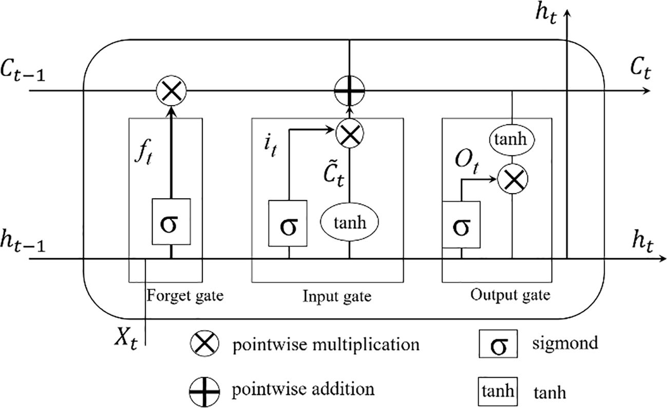
LSTM improves the efficiency of information transfer from the previous cell to the next cell in the same layer by adding a “gate” data structure (Wang et al., 2023; Zhou et al., 2023). The main structure of the model is composed of forget gate, input gate, and output gate, and the internal structure of the model is shown in Figure 1. In the forget gate, except that the initial value of the cell at the first time is manually set, the cell at other times needs to obtain the cell state C_t−1 of the previous cell, and then compare it with the current input vector information X_i, and the value range [0,1] is obtained by activating the function sigmoid. If the corresponding position of the vector is 0, it means that the corresponding position information of the previous time is forgotten, and if it is 1, the information memory of the corresponding position is performed. The forget gate filters the input data and passes it to the input gate. The relevant formulas for the LSTM prediction model refer to Xu et al. (2023).

Figure 1

Figure 1. Network structure of LSTM.

2.2.5.2 RF model

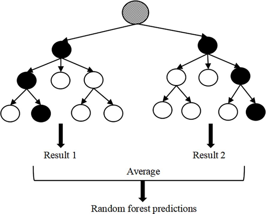
RF is an ensemble learning algorithm that constructs multiple decision trees as base learners using the bootstrap aggregating (bagging) strategy to classify and predict outcomes. By randomly selecting subsets of features, RF effectively addresses high-dimensional data, thereby reducing dimensionality and enhancing model efficiency. Additionally, RF’s feature importance ranking further improves the model’s generalization ability. Random forest (RF) model (Yang et al., 2015) is a learning method based on classification decision tree, with the minimum number of leaves set to 1, the minimum number of splits set to 1, and the number of decision trees set to 500. The fundamental workflow of the RF algorithm is illustrated in Figure 2, with detailed principles and steps described by Hou (2024).

Figure 2

Figure 2. Flow chart of random forest.

2.2.5.3 BP neural network model

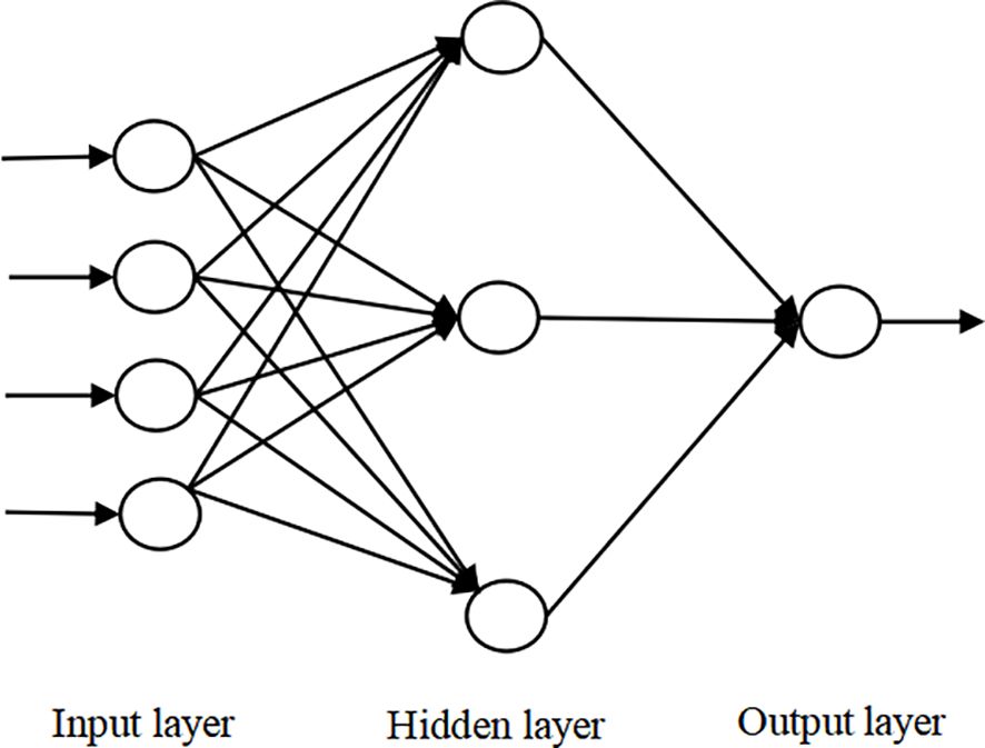
A BP neural network typically consists of multiple layers, including an input layer, hidden layers, and an output layer. Its learning process operates in two stages: forward propagation of signals and backward propagation of errors. During forward propagation, input data passes through the input layer, is processed by the hidden layers, and then reaches the output layer. If the actual output deviates from the expected output, backward propagation is triggered, where the output error is propagated backward through the network. This error is distributed across all units in each layer, providing the basis for adjusting the weights of the network. The process of forward signal propagation, backward error propagation, and weight adjustment repeats iteratively until the network output error reaches an acceptable threshold or a predetermined number of learning iterations is completed. The topological structure of the BP neural network is shown in Figure 3, while the underlying principles and algorithmic steps are detailed in Xiao (2021).

Figure 3

Figure 3. Topological structure of three-layer BP neural network.

2.2.5.4 XGBoost model

The XGBoost model, an enhancement of the gradient boosting decision tree model, consists of multiple decision trees arranged iteratively. During the tree-building process, the XGBoost algorithm automatically determines the optimal splitting directions, making it highly effective in handling missing values often present in fisheries production data. The detailed principles and methodology of the XGBoost algorithm can be found in Zhang et al. (2024).

2.2.5.5 SSA-XGBoost model

The sparrow search algorithm simulates the foraging and anti-predation behaviors of sparrow populations (Xu and Zhao, 2023), taking inspiration from Particle Swarm Optimization (PSO) and Ant Colony Optimization (ACO). Unlike ACO, which has a slower search speed, and PSO, which is prone to premature convergence, SSA offers superior performance in terms of search accuracy, convergence speed, stability, and the ability to avoid local optima. The principles and steps of the SSA-XGBoost model are detailed in Yuan et al. (2022).

2.2.5.6 Validation of model prediction results

In this study, the lagged data of climate factors were used as training data, and the catch data of bigeye tuna were used as prediction data. To achieve this, cross-validation method was employed. Of the data, 70% were randomly selected as training set and 30% were used as test set. LSTM, RF, BP, XGBoost, and SSA-XGBoost models were used for prediction. The accuracy of the predicted values was verified and compared by using mean absolute error (MAE) and root mean squared error (RMSE). MAE is the average absolute error between the predicted values and the actual values, and the smaller the value, the higher the prediction accuracy. RMSE is the sample standard deviation between the predicted values and the actual values, and the smaller the value, the smaller the dispersion. The error calculation formula (Yuan et al., 2022) is as follows:

$\begin{array}{ll}{X}_{MAE}=\frac{1}{n}\times {\displaystyle \sum _{t=1}^n|D_t-P_t|}& (6)\end{array}$

$\begin{array}{ll}{X}_{RMSE}=\sqrt{\frac{1}{\text{n}}\times {\displaystyle \sum _{t=1}^n{(D_t-P_t)}^2}}& (7)\end{array}$

where X_MAE is the mean absolute error, X_RMSE is the root mean squared error, D_t is the predicted catch of bigeye tuna at time t, P_t is the actual catch of bigeye tuna in year t, and n is the number of test sets.

3 Results and analysis

3.1 Data and data preprocessing

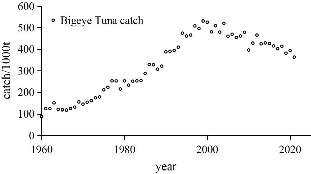
Global bigeye tuna catch data (Figure 4) indicate that the catch volume of bigeye tuna has shown a linear increase since 1960, reaching a historical peak in 1999. Subsequently, the catch volume has exhibited a fluctuating decline, continuing through to 2021.

Figure 4

Figure 4. Time series of bigeye tuna catch.

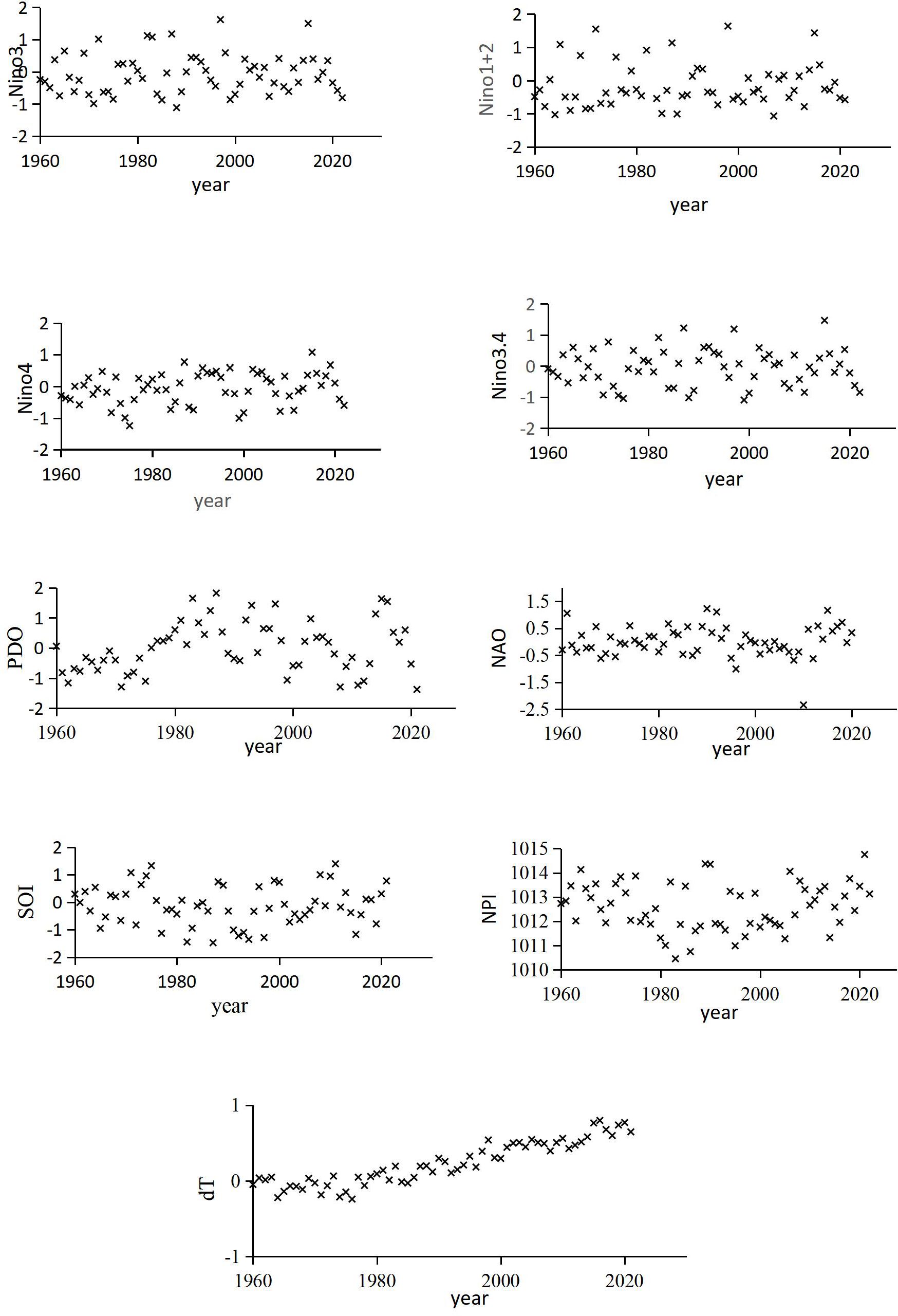
The time series of climate change characterization factors are shown in Figure 5. It is evident that over the period from 1960 to 2021, dT exhibits an undulating upward trend. The PDO shows an alternating pattern of warm and cold phases with a cycle of approximately 40 years. The other climate change indicators demonstrate shorter variation cycles. The results indicate that, apart from the dT data, the remaining factors primarily oscillate around a parallel baseline.

Figure 5

Figure 5. Time series of characterization factors of climate.

3.2 Correlation analysis of climate change characterization factors

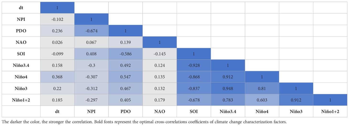
From Table 1, it can be seen that the correlation coefficients among Niño1 + 2, Niño3, Niño4, and Niño3.4 are high, with the exception of Niño1 + 2 and Niño4, which have a correlation coefficient of 0.603. The absolute values of the correlation coefficients among the other factors exceed 0.7, indicating a high correlation. The SOI also has correlation coefficients with Niño3, Niño4, and Niño3.4 that exceed 0.7, further indicating high correlation. To select representative factors from the highly correlated climate indices, Niño1 + 2, Niño3, Niño4, and Niño3.4 were considered as one set, and SOI, Niño3, Niño4, and Niño3.4 as another. Given that Niño3, Niño4, and Niño3.4 appear in both sets, Niño1 + 2, SOI, NAO, PDO, NPI, and dT were chosen as the six relatively independent climate indices to ensure the independence of the factors.

Table 1

Table 1. Spearman rank correlation coefficient result.

3.3 Lag years of climate change characterization factors

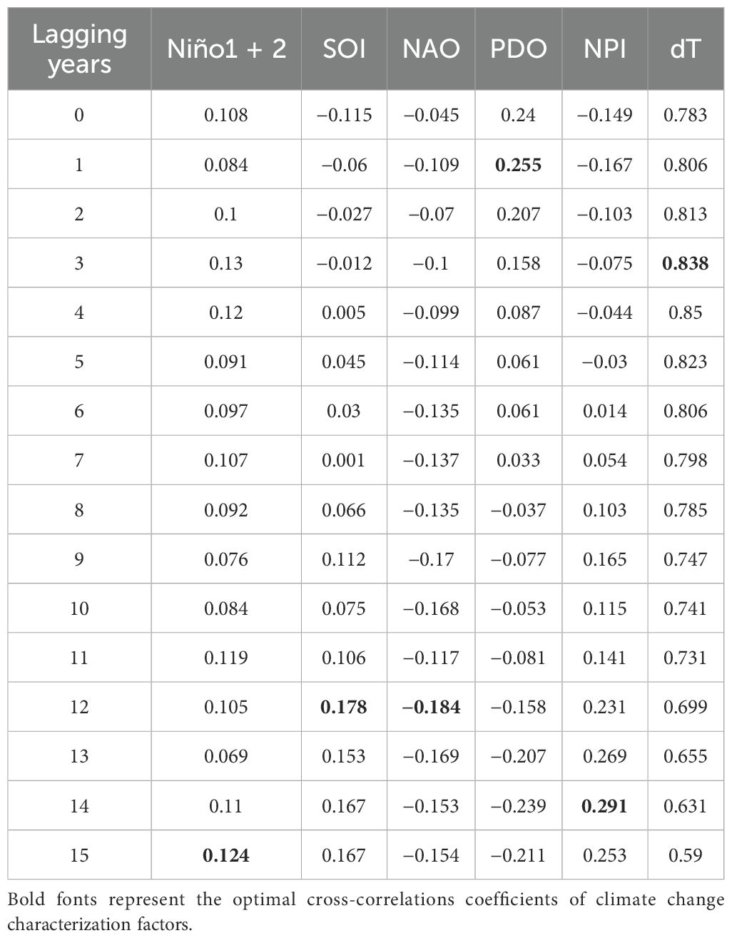
The optimal lag for each climate change indicator is determined by the lag at which the cross-correlation coefficient reaches its maximum absolute value. As shown in Table 2, the optimal lag years for the climate change indicators Niño1 + 2, SOI, NAO, PDO, NPI, and dT are 15 years, 12 years, 12 years, 1 year, 14 years, and 4 years, respectively. The ratios of the absolute cross-correlation coefficients at the optimal lag years to those at 0 years are as follows: Niño1 + 2 is 1.15 times, SOI is 1.55 times, NAO is 4.09 times, PDO is 1.06 times, NPI is 1.95 times, and dT is 1.09 times. The absolute values of the cross-correlation coefficients between Niño1 + 2, SOI, NAO, PDO, NPI, and bigeye tuna are all below 0.3. The results indicate that the influence of the climate change indicators at their optimal lag years on bigeye tuna catch is greater than that with a 0-year lag.

Table 2

Table 2. Mutual correlation between climate change characterization factors and catch.

3.4 Relative importance of climate change characterization factors

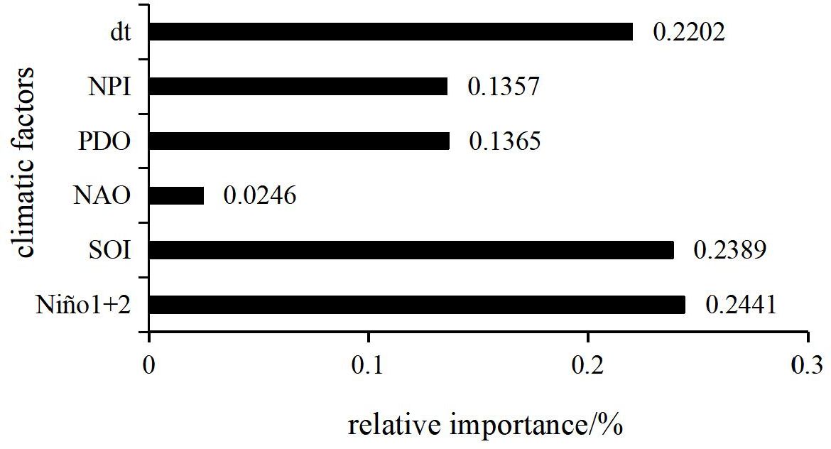
From Figure 6, it is evident that the relative importance of climate change indices on catch follows the order: Niño1 + 2, SOI, dT, PDO, NPI, and NAO. There is a significant difference between the importance of Niño1 + 2, SOI, dT, and that of PDO, NPI, and NAO. The combined importance of the climate indices Niño1 + 2, SOI, and dT accounts for approximately 70%. Therefore, the climate indices Niño1 + 2, SOI, and dT can be considered the key climate factors affecting the catch of bigeye tuna.

Figure 6

Figure 6. Relative importance of climate change characterization factors.

3.5 Model comparison and validation of predicted catch of bigeye tuna

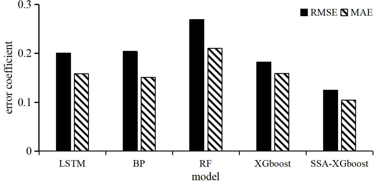
The error statistics from different models (Figure 7) indicate that the SSA-XGboost model has the lowest MAE and RMSE compared to other prediction models, demonstrating its superior predictive performance. The RF model has the highest MAE and RMSE among the five models, indicating its relatively poor predictive performance. The predictive performance of the LSTM and BP models is similar, but slightly inferior to that of the XGboost model. Overall, the SSA-XGboost model exhibits the best predictive performance for bigeye tuna catch among the five models.

Figure 7

Figure 7. Statistical results of prediction errors of different models.

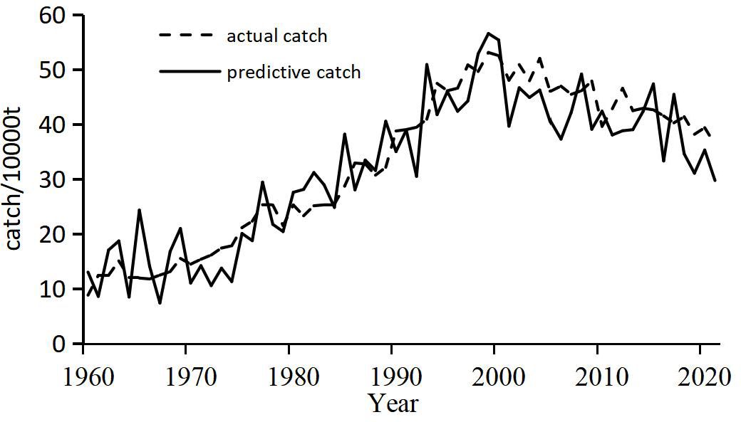
As illustrated in Figure 8, the predicted catch trend of bigeye tuna closely aligns with the observed trend over the analyzed period, capturing significant features such as the increase in catch around 2000 and its subsequent peak. Both the predicted and actual data display a consistent pattern of rising catch levels followed by a decline. While the predicted values exhibit larger fluctuations than the actual catch data, the overall variation range remains reasonable. Specifically, the ratio of the maximum to minimum values for actual catches is approximately 6, while the predicted values have a similar ratio of 7.6. This numerical similarity supports the model’s effectiveness in capturing the overall range of catch data.

Figure 8

Figure 8. Comparison between predicted and actual catch.

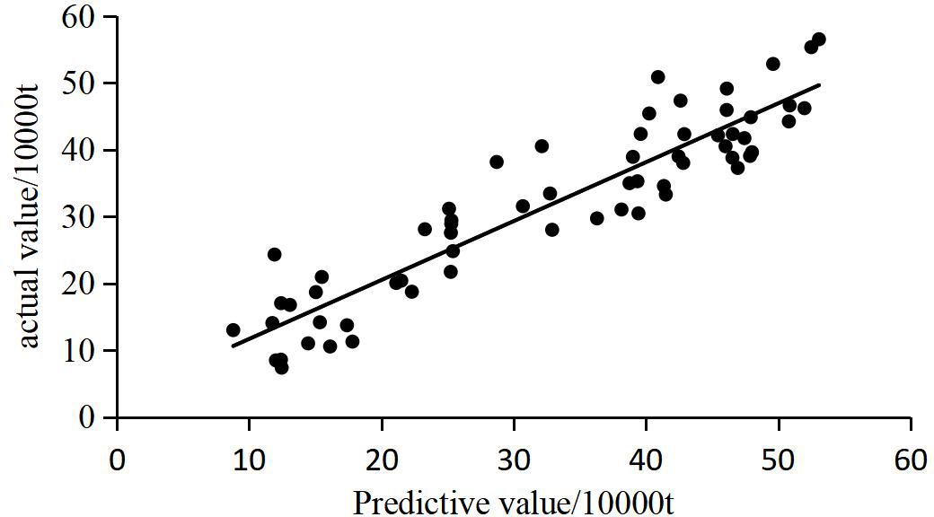
To further validate the model’s predictive accuracy, a linear regression between the predicted and actual catch values was performed, as shown in Figure 9. The results reveal a strong linear correlation between the predicted and actual values, with points closely clustering around the fitted line. This relationship highlights the close alignment between predicted and observed catch levels. Additionally, the R² value of 0.853, with a significance level of <0.001, underscores the high predictive capability of the SSA-XGBoost model for bigeye tuna catch. The regression equation, y=0.968x+20324, further demonstrates the model’s robustness in predicting catch values.

Figure 9

Figure 9. Linear fitting relationship between predicted and actual catch.

4 Discussion

In this study, the Spearman rank correlation analysis was used to select six independent climate change characterization factors, including Niño1 + 2, SOI, NAO, PDO, NPI, and dT. The optimal lag years of these factors in relation to the catch of bigeye tuna were found to be 15 years, 12 years, 12 years, 1 year, 14 years, and 4 years, respectively. The longest lag year was for Niño1 + 2 (15 years), while the shortest was for PDO (1 year). This is different from the 3-month lag years of ENSO observed in Lu’s study (Lu et al., 2001), which might be due to the long duration and wide range of the catch of bigeye tuna used in this study. This also confirms the lag effect of climate change on fisheries, which may be due to the indirect impact of climate change on fisheries through changes in the marine environment (Yu and Wen, 2022). The lag phenomenon may be attributed to the lag effects of climate change on marine and climate factors, food supply, survival rate of larvae, and habitats, which subsequently influence the spawning and recruitment of bigeye tuna (Fang et al., 2008), thus affecting their catches. Furthermore, studies have found that the distribution (Hampton, 1997; Hampton et al., 1999), reproduction (Bakun and Parrish, 1990), catch yield (Torres-Orozco et al., 2006; Deary et al., 2015), and spatial distribution (Ding et al., 2024) of fish populations are closely related to these factors.

The three main climate change characterization factors that affect the catch of bigeye tuna are Niño1 + 2, dT, and SOI, accounting for approximately 70% of the six climate change characterization factors. These findings are generally consistent with the results of other scholars (Zhou et al., 2004), indicating that the El Niño-Southern Oscillation phenomenon has a significant impact on the bigeye tuna fishery. This may be attributed to the fact that bigeye tuna is a warm-water species that is greatly influenced by temperature (Huang et al., 2020), having specific requirements for water temperature during their habitat and spawning periods. During El Niño, the upper boundary of the thermocline is shallower and weaker compared to La Niña, resulting in a smaller suitable habitat, which leads to higher catch of bigeye tuna in La Niña years. Meanwhile, during El Niño, the reproduction of plankton decreases, reducing the nutrient content in the water column (Huang et al., 2020), resulting in less nutrition for bigeye tuna and lower catches. Conversely, in La Niña years, the proliferation of plankton increases, improving the nutrient content of the water column, allowing bigeye tuna to obtain more nutrition, and leading to higher catches. In terms of the sea–air temperature anomaly index (dT), climate change affects the recruitment of fish populations by influencing sea water temperature (Sirabella et al., 2001; Ottersen and Stenseth, 2001). The lag phenomenon may be due to the indirect effects of climate factors on the catch of bigeye tuna through influencing marine and climate factors, recruitment, habitats, and spatial–temporal distribution, thus exhibiting a certain degree of lag.

Numerous researchers have applied various models to predict fisheries trends, with most relying on traditional regression models. For example, the BP neural network model (Ding et al., 2021a, 2021b) achieves predictions by iteratively adjusting the weights between neurons and increasing the number of hidden layers based on empirical knowledge. The Bayesian method (Chen et al., 2013) imposes strict requirements on the dependent variable, and the complex, non-linear relationships between environmental and climate factors and fisheries can greatly influence prediction accuracy. Additionally, models like GLM and GAM require researchers to have a thorough understanding of the error distribution in fisheries data and the transformation of predictive variables (Guan and Chen, 2009), as any misinterpretation can easily affect the results. In contrast, the XGBoost model used in this study is a modern ensemble learning approach (Li et al., 2023) that effectively mitigates overfitting, even with small sample sizes and numerous variables. Unlike traditional decision tree models, XGBoost has the advantage of automatically learning optimal splitting directions. The enhanced SSA-XGBoost model further reduces data complexity and achieves rapid convergence by incorporating climate change factors, enabling accurate predictions of bigeye tuna catches. Results indicate that the optimized predictions using the SSA were significantly better than those of the standalone XGBoost model, with a reduction in RMSE by 0.058 and MAE by 0.055. This study provides valuable insights into the integration of different regression models for fisheries prediction and presents a novel approach to modeling fisheries data.

This study explored the impact of climate change characterization factors as the only influencing factors on the catch of bigeye tuna, highlighting the importance of climate factors in fisheries. This is consistent with the proposal by some scholars (Ormaza-González et al., 2016) to use climate factors to help manage fisheries and plan for the industry in the long term. The climate factors selected in this study, including Niño1 + 2, SOI, NAO, PDO, NPI, and dT, have significant impacts on fisheries, as reported by previous studies. For example, Yang et al. (2019). found that the ENSO phenomenon has a significant impact on the spatial distribution and resource abundance of Chilean jack mackerel; Sirabella et al. (2001) found that NAO affects the recruitment of cod by influencing sea water temperature, and Ottersen and Stenseth (2001) reached similar conclusions. Li et al. (2020) reported a close relationship between the population abundance of yellow croaker and PDO, while Carey et al. (2017) found a strong correlation between the migration duration of red salmon and NPI. The IPCC report (Intergovernmental Panel on Climate Change (IPCC), 2007) also points out that the continuous increase in ocean temperature during the period of 1971–2010 has led to an increase in atmospheric temperature. By discussing the long-term impact of climate change on the catch of bigeye tuna from the angle of climate change with a long time series, this study can provide scientific evidence for the sustainable development of the bigeye tuna fishery and understand the long-term impact of climate change on bigeye tuna. This study investigates the effect of climate change factors as the sole influencing factor on the catch of bigeye tuna, highlighting the climatic reasons behind the variations in the abundance of bigeye tuna resources and fishing grounds. This approach differs from those that consider climate change characterization factors as one of the influencing factors or discuss the issue during climate transitions. Moreover, the use of long-term (low-frequency) climate change parameters to study the impact on bigeye tuna is distinct from short-term research focusing on marine environmental factors. The findings of this study can provide a reference for China to develop scientific and effective fishery management measures for bigeye tuna. However, it is worth noting that due to the lack of data such as fishing gear information and operating hours, there are limitations in calculating catch per unit effort (CPUE). Future research could continue to delve deeper into this area after supplementing relevant data.

Data availability statement

Publicly available datasets were analyzed in this study. This data can be found here: https://www.esrl.noaa.gov, https://www.metoffice.gov.uk, https://www.wcpfc.int/doc/wcpfc-tuna-fishery-yearbook-2021.

Author contributions

PD: Conceptualization, Data curation, Formal analysis, Investigation, Methodology, Resources, Validation, Visualization, Writing – original draft. HX: Data curation, Methodology, Formal analysis, Validation, Writing – review & editing. XRZ: Methodology, Resources, Supervision, Validation, Writing – review & editing. SYD: Supervision, Writing – review & editing. SQB: Supervision, Writing – review & editing.

Funding

The author(s) declare that financial support was received for the research, authorship, and/or publication of this article. This work was supported by Collection of Fishery Production Data (D-8002-12-0127-2) and Integrated intelligent equipment for efficient fishing and shipborne processing in deep-sea fisheries (D-8006-23-0016).

Conflict of interest

The authors declare that the research was conducted in the absence of any commercial or financial relationships that could be construed as a potential conflict of interest.

Publisher’s note

All claims expressed in this article are solely those of the authors and do not necessarily represent those of their affiliated organizations, or those of the publisher, the editors and the reviewers. Any product that may be evaluated in this article, or claim that may be made by its manufacturer, is not guaranteed or endorsed by the publisher.

References

Bakun A., Parrish R. H. (1990). Comparative studies of coastal pelagic fish reproductive habitats: the Brazilian sardine (Sardinella aurita). ICES J. Mar. Sci. 46, 269–283. doi: 10.1093/icesjms/46.3.269

Crossref Full Text | Google Scholar

Cao X. Y., Zhou W. F., Fan W., Li S. ,. F. (2009). Analysis on barycenter of fishing ground for bigeye tuna and yellowfin tuna by longline in the Indian Ocean. J. Shanghai Ocean Univ. 18, 466–471. Available online at: http://shhydxxb.ijournals.cn/shhy/article/abstract/20090478

Google Scholar

Carey M. P., Zimmerman C. E., Keith K. D., Schelske M., Lean C., Douglas D. C. (2017). Migration trends of sockeye salmon at the northern edge of their distribution. Trans. Am. Fisheries Soc. 146 (4), 791–802. doi: 10.1080/00028487.2017.1302992

Crossref Full Text | Google Scholar

Chen X. J., Gao F., Guan W. J., Lei L., Wang J. ,. T. (2013). Review of fishery forecasting technology and its models. J. Fisheries China 37, 1270–1280. doi: 10.3724/SP.J.1231.2013.38313

Crossref Full Text | Google Scholar

Deary A. L., Moret-Ferguson S., Engels M., Zettler E., Jaroslow G., Sancho G. (2015). Influence of central Pacific oceanographic conditions on the potential vertical habitat of four tropical tuna species1. Pacific Sci. 69, 461–475. doi: 10.2984/69.4.3

Crossref Full Text | Google Scholar

Ding P., Zou X. R., Bai S. Q., Zhang P. (2021a). Spatial and temporal analysis of Chilean jack mackerel fishing ground and its resource abundance prediction in the Southeast Pacific. J. Dalian Ocean Univ. 36, 629–636. doi: 10.16535/j.cnki.dlhyxb.2020-216

Crossref Full Text | Google Scholar

Ding P., Zou X. R., Ding S. Y., Bai S. Q. (2024). Study on the relationship between catch of thunnus albacares and climatic factors based on CNN-BiLSTM model. South China Fisheries Sci. 20, 19–26. doi: 10.12131/20230190

Crossref Full Text | Google Scholar

Ding P., Zou X. R., Feng C., Bai S. Q. (2021b). Analysis of migratory route of Chilean jack mackerel in the Southeast Pacific. J. Dalian Ocean Univ. 36, 1027–1034. doi: 10.16535/j.cnki.dlhyxb.2021-029

Crossref Full Text | Google Scholar

Duparc A., Aragno V., Depetris M., Floch L., Cauquil P., Lebranchu J., et al. (2020). Assessment of the species composition of major tropical tuna s in purse seine catches: a new modelling approach for the tropical tuna treatment processing Available online at: https://www.iccat.int/Documents/CVSP/CV076_2019/n_6/CV076060951.pdf (case of the French fleet in Atlantic Ocean), Collect. Vol. Sci. Pap. ICCA 76, 951–982.

Google Scholar

Fang H., Zhang H., Liu F., Zhou W. F. (2008). A summary of research progress related with the fluctuation of the worldwide main marine fishery resources influenced by climate changes. Mar. Fisheries 04), 363–370. doi: 10.3969/j.issn.1004-2490.2008.04.012

Crossref Full Text | Google Scholar

Feng B., Chen X. J., Xu L. X. (2009). Multivariate quantile regression on habitat suitability Index of Thunnus obesus in the Indian Ocean. J. Guangdong Ocean Univ. 29, 48–52. doi: 10.3969/j.issn.1673-9159.2009.03.010

Crossref Full Text | Google Scholar

Friedland K. D., Boucher J. M., Jones A. W., Methratta E. T., Morse R. E., Foley C., et al. (2023). The spatial correlation between trawl surveys and planned wind energy infrastructure on the US Northeast Continental Shelf. ICES J. Mar. Sci., 1, 12. doi: 10.1093/icesjms/fsad167

Crossref Full Text | Google Scholar

Gan Y., Ma X. C., Yan J. (2019). The application of spatial cross correlation in analyzing the migration of submarine sand waves. Haiyangxuebao 41, 42–52. doi: 10.3969/ji.ssn.0253-4193.2019.04.004

Crossref Full Text | Google Scholar

Gilman E., Chaloupka M. (2024). Evidence from interpretable machine learning to inform spatial management of Palau's tuna fisheries. Ecosphere 15, e4751. doi: 10.1002/ecs2.4751

Crossref Full Text | Google Scholar

Guan W. J., Chen X. J. (2009). Fishing efficiency for mackerel and scad in the large light purse seine fishery estimated by generalized linear model. J. Fisheries China 33, 221–227. doi: 10.3321/j.issn:1000-0615.2009.02.008

Crossref Full Text | Google Scholar

Hampton J. (1997). Estimates of tag-reporting and tag-shedding rates in a large-scale tuna tagging experiment in the western tropical Pacific Ocean. Oceanographic Literature Rev. 11, 1346.

Google Scholar

Hampton J., Lewis A., Williams P. (1999). The western and central Pacific tuna fishery: overview and status of stocks (New Caledonia: Secretariat of the Pacific Community). Oceanic fisheries programme.

Google Scholar

Hoshino E., Pascoe S., Schrobback P., McWhinnie S., Curtotti R. (2024). Long-run productivity changes in the Australian Northern prawn fishery. Fisheries Res. 273, 106969. doi: 10.1016/j.fishres.2024.106969

Crossref Full Text | Google Scholar

Hou Q. L. (2024). Research on intelligent recognition system of tuna purse seine shoal based on machine vision technology (Shanghai Ocean University). doi: 10.27314/d.cnki.gsscu.2024.000002

Crossref Full Text | Google Scholar

Huang J. L., Dai L. B., Wang X. F., Zhou C., Tang, Hao (2020). Spatio-temproal distribution pattern of habitat preference of bigeye tuna free-swimming schools in the eastern Pacific Ocean. J. Shanghai Ocean Univ. 29, 889–898. doi: 10.12024/jsou.20191202874

Crossref Full Text | Google Scholar

Intergovernmental Panel on Climate Change (IPCC) (2007). “Climate change 2007: synthesis report,” in Contribution of Working Groups I, II and III to the Fourth Assessment Report of the Intergovernmental Panel on Climate Change. Eds. Pachauri R. K., Reisinger A. (IPCC, Geneva, Switzerland), 104pp. Core Writing Team.

Google Scholar

Li J. Y., Li Y., Huang L. Q., Wang H. X., Li C. R. (2023). Piecewise wind power forecast based on the XGBoost-GRNN algorithm. Comput. Integrated Manufacturing Syst. 30 (06), 2172–2185. doi: 10.13196/j.cims.2021.0799

Crossref Full Text | Google Scholar

Li H., Yang S., Tang Q., Zhou X., Sun Y. (2020). Long-term variation in the abundance of Pacific herring (Clupea pallasii) from the Yellow Sea in the western North Pacific and its relation to climate over the past 590 years. Fisheries Oceanography 29, 56–65. doi: 10.1111/fog.12449

Crossref Full Text | Google Scholar

Lu H. J., Lee K. T., Lin H. L., Liao C. H. (2001). Spatio-temporal distribution of yellowfin tuna Thunnus albacares and bigeye tuna Thunnus obesus in the Tropical Pacific Ocean in relation to large-scale temperature fluctuation during ENSO episodes. Fisheries Sci. 67, 1046–1052. doi: 10.1046/j.1444-2906.2001.00360.x

Crossref Full Text | Google Scholar

MacDonnell M., Vandergeest P. (2024). Fisher experience on distant water fishing vessels: the implications of variation by vessel type for employment standards. Maritime Stud. 23, 1–17. doi: 10.1007/s40152-024-00365-1

Crossref Full Text | Google Scholar

Mao J. M., Chen X. J., Jing Y. (2016). Forecasting fishing ground of Thunnus alalunga based on BP neural network in the South Pacific Ocean. Haiyangxuebao 38, 34–43. doi: 10.3969/j.issn.0253-4193.2016.10.004

Crossref Full Text | Google Scholar

Ormaza-González F. I., Mora-Cervetto A., Bermúdez-Martínez R. M., Hurtado-Domínguez M. A., Peralta-Bravo M. R., Jurado-Maldonado V. M. (2016). Can small pelagic fish landings be used as predictors of high-frequency oceanographic fluctuations in the 1–2 El Niño region? Adv. Geosciences 42, 61–72. doi: 10.5194/adgeo-42-61-2016

Crossref Full Text | Google Scholar

Ottersen G., Stenseth N. C. (2001). Atlantic climate governs oceanographic and ecological variability in the Barents Sea. Limnology Oceanography 46, 1774–1780. doi: 10.4319/lo.2001.46.7.1774

Crossref Full Text | Google Scholar

Pachauri R. K., Allen M. R., Barros V. R., Broome J., Cramer W., Christ R., et al. (2014). “Climate change 2014: synthesis report,” in Contribution of Working Groups I, II and III to the Fifth Assessment Report of the Intergovernmental Panel on Climate Change. Eds. Pachauri R., Meyer L. (IPCC, Geneva, Switzerland), 151.

Google Scholar

Sirabella P., Giuliani A., Colosimo A., Dippner J. W. (2001). Breaking down the climate effects on cod recruitment by principal component analysis and canonical correlation. Mar. Ecol. Prog. Ser. 216, 213–222. doi: 10.3354/meps216213

Crossref Full Text | Google Scholar

Song L. M., Gao P. F., Zhou Y. Q., Zhang Y. (2007). Habitat environment integration index of Thunnus obesus in the high seas of the Central Atlantic Ocean based on the quantile regression. J. Fisheries China 06), 798–804. doi: 10.3724/SP.J.00001

Crossref Full Text | Google Scholar

Song L. M., Ren S. Y., Hong Y. R., Zhang T. J., Sui H. S., Li B., et al. (2022). Comparison on fishing ground forecast models of Thunnus alalunga in the tropical waters of Atlantic Ocean. Oceanologia Limnologia Sin. 53, 496–504. doi: 10.11693/hyhz20211000253

Crossref Full Text | Google Scholar

Song L. M., Ren S. Y., Zhang M., Sui H. ,. S. (2023). Fishing ground forecasting of bigeye tuna (Thunnus obesus) in the tropical waters of Atlantic Ocean based on ensemble learning. J. Fisheries China 47, 64–76. doi: 10.11964/jfc.20210312692

Crossref Full Text | Google Scholar

Sun C. H., Maunder M. N., Pan M., Aires-da-Silva A., Bayliff W. H., Compeán G. A. (2019). Increasing the economic value of the eastern Pacific Ocean tropical tuna fishery: Tradeoffs between longline and purse-seine fishing. Deep Sea Res. Part II: Topical Stud. Oceanography 169, 104621. doi: 10.1016/j.dsr2.2019.07.009

Crossref Full Text | Google Scholar

Torres-Orozco E., Muhlia-Melo A., Trasviña A., Ortega-García S. (2006). Variation in yellowfin tuna (Thunnus albacares) catches related to El Niño-Southern Oscillation events at the entrance to the Gulf of California. Fishery Bull. 104, 197–203.

Google Scholar

Wang H., Ding F., Wu X., Li Y., Wei C. G., Liu Q. Y., et al. (2023). Prediction method of airline passenger incoming calls based on LSTM neural network. J. Civil Aviation 7, 136–140+131. doi: 10.3969/j.issn.2096-4994.2023.05.030

Crossref Full Text | Google Scholar

Xiao Q. H. (2021). Study on the assessment model of Chilean Jack mackerel resources in the Southeast Pacific Ocean under the background of climate change. Shanghai Ocean Univ. 2021, 16–42. doi: 10.27314/d.cnki.gsscu.2020.000001

Crossref Full Text | Google Scholar

Xiao Q. H., Huang S. L. (2021). Impact of climate change on Chilean jack mackerel catch in the Southeast Pacific. J. Fishery Sci. China 28 (08), 1020–1029. doi: 10.12264/JFSC2020-0323

Crossref Full Text | Google Scholar

Xu H., Song L., Zhang T., Li Y., Shen J., Zhang M., et al. (2023). Effects of different spatial resolutions on prediction accuracy of thunnus alalunga fishing ground in waters near the Cook Islands based on long short-term memory (LSTM) neural network model. J. Ocean Univ. China 22, 1427–1438. doi: 10.1007/s11802-023-5525-5

Crossref Full Text | Google Scholar

Xu Z. H., Zhao Y. D. (2023). SSA-BP model for predicting water contents in stem integrating multiple environmental factors acquired via IoT. Trans. Chin. Soc. Agric. Eng. 39 (16), 150–159. doi: 10.11975/j.issn.1002-6819.202304150

Crossref Full Text | Google Scholar

Yang S. L., Zhang S. M., Jiang X. W., Zou B., Hua C. ,. J., Zhou W. ,. F. (2013). Temporal and spatial variation characteristics of the thermocline in Thunnus obesus and Thunnus albacares fishing grounds in the tropical Atlantic Ocean. J. Appl. Oceanography 32, 349–357. doi: 10.3969/J.ISSN.2095-4972.2013.03.007

Crossref Full Text | Google Scholar

Yang S. L., Zhang Y., Zhang H., Fan W. (2015). Comparison and analysis of different model algorithms for CPUE standardization in fishery. Trans. Chin. Soc. Agric. Eng. 31, 259–264. doi: 10.11975/j.issn.1002-6819.2015.21.034

Crossref Full Text | Google Scholar

Yang X. S., Zou X. R., Xu X. X., Wang Z. A. (2019). Effects of ENSO on abundance index and spatial-temporal change of Chilean jack mackerel in the Southeast Pacific Ocean. J. Shanghai Ocean Univ. 28, 290–297. doi: 10.12024/jsou.20180902406

Crossref Full Text | Google Scholar

Yu W., Wen J. (2022). Review on the response of important fishery resources to the climatic and environment variability in the Humboldt Current System. J. Shanghai Ocean Univ. 31, 620–630. doi: 10.12024/jsou.20220203709

Crossref Full Text | Google Scholar

Yuan H. C., Gao Z. Y., Zhang T. J. (2022). Prediction of albacore tuna abundance in south Pacific based on improved XGBoost model. Trans. Oceanology Limnology 44, 112–120. doi: 10.13984/j.cnki.cn37-1141.2022.02.015

Crossref Full Text | Google Scholar

Zhang M. X., Chen B., Liu W. Q., Qi Y. N., Zhang M. (2024). Dam deformation prediction model selected by SSA-XGBoost and temporal and spatial features. J. Hydroelectric Eng. 43, 84–98. doi: 10.11660/slfdxb.20240108

Crossref Full Text | Google Scholar

Zhang C., Zhou W. F., Tang F. H., Shi Y. ,. C., Fan W. (2022). Forecasting models for yellowfin tuna fishing ground in the central and western Pacific based on machine learning. Trans. Chin. Soc. Agric. Eng. 38, 330–338. doi: 10.11975/j.issn.1002-6819.2022.15.036

Crossref Full Text | Google Scholar

Zhou S., Shen J. H., Fan W. (2004). Impacts of the El Nino Southern Oscillation on skipjack tuna purse-seine fishing grounds in the Western and Central Pacific Ocean. Mar. Fisheries. 12 (6), 739–744. doi: 10.3969/j.issn.1004-2490.2004.03.002

Crossref Full Text | Google Scholar

Zhou K., Jiao L. X., Hu Z. J., Yan L. X., Bi R. Y., Wang Y. J. (2023). Automatic verification method of operation ticket based on attention mechanism of CNN-BiLSTM. Eng. J. Wuhan Univ. 56, 1114–1123. doi: 10.14188/j.1671-8844.2023-09-011

Crossref Full Text | Google Scholar

Zhou Y. J., Yao Y. B., Xiong Y. L., Shan L. (2020). Study of correlation between PWV and PM_2.5 based on Spearman rank correlation coefficient. J. Geodesy Geodynamics 40, 236–241. doi: 10.14075/j.jgg.2020.03.004

Crossref Full Text | Google Scholar