Comparison of linear and nonlinear modeling approaches to develop an abundance index based on voyage and market data for a data-limited fishery

Introduction: Worldwide coastal fish resources face severe threats from fisheries overexploitation. However, the evaluation of abundance trends in most coastal fisheries is constrained by limited data. This study took blackmouth croaker (Atrobucca nibe), a stock depleted by coastal trawl fishery in southwestern Taiwan, as an example to showcase the development of a relative abundance index from data-limited fishery (only landing data were available).

Methods: This study employed unique data sourcing from voyage data recorders (VDRs) to estimate fishing effort (in combination with landing data to estimate the catch per unit effort, CPUE) that demonstrated the potential application in global data-limited fisheries and assessed alternative approaches for predictors of fishery-targeting practices to condition effort for producing more accurate metrics of relative abundance. The nominal CPUE was standardized using three statistical models: generalized linear model, generalized additive model (GAM), and vector-autoregressive spatiotemporal models (VASTs) with two treatments of each of the four effects: environmental (sea temperature, salinity, density of mixing layer, seafloor temperature, and chlorophyll), vessel, spatial, and targeting effects. A total of 15 models were designed and compared for these effects, and their explanatory power (EP) was evaluated using cross-validation R² and other metrics.

Results and discussion: Results indicated that the targeting effect exerted the most significant influence on standardization and was suggested to be addressed through the principal component analysis (PCA) approach. Both vessel and spatial effects demonstrated considerable influence, whereas the environmental effect exhibited a limited impact, possibly due to the small fishing area in this study. Regarding models’ EP, given the nonlinear nature of the PCA algorithm and environmental data, the study highlighted the superiority of the GAM over linear-based models. However, incorporating nonlinear features in VAST (M15) makes it the most effective model in terms of predictive power in this study. Concerning the stock status, despite variations in relative CPUE trends among major models, a general declining trend since 2015 signals the potential decline of the blackmouth stock and urges fishery managers to consider further design of management measures.

1 Introduction

Coastal marine ecosystems, renowned for their high productivity, face severe threats from pervasive human disturbance, with overfishing emerging as a primary concern leading to the depletion of fish stocks (Jackson et al., 2001; Halpern et al., 2008; Nias, 2013). Many data-rich stocks have been assessed with sophisticated approaches, such as stock assessments, and managed accordingly with strengthened measures. Recent analyses suggested a global recovery of the population of well-managed stocks (Duarte et al., 2020; Hilborn et al., 2020), although this is cautioned to be over-optimistic (Duarte et al., 2020). In contrast, many coastal fisheries lack proper management due to insufficient data, creating uncertainty about stock depletion levels and posing challenges in persuading stakeholders to implement necessary measures, such as reducing fishing efforts (King, 2007). The absence of adequate data is attributed to various factors, notably the frequent omission of small-scale coastal fisheries from logbook submission requirements, which hinders the derivation of comprehensive geo-referenced effort data (Chang et al., 2019; Sari et al., 2021).

Various alternative approaches can be explored to address the issue, especially in obtaining abundance indices that provide insights into population abundance changes over time (Chang et al., 2017; Ducharme-Barth et al., 2018). Utilizing market landing data, which includes date information and vessel identity and adheres to specific data quality standards (e.g., minimal discarding due to size-specific high grading, at-sea dumping, and losses during fish processing), can serve as a substitute to represent the catch (Afonso-Dias et al., 2004; Lourenço and Pereira, 2006; Bastardie et al., 2010; FAO, 2023). Fishing effort can be estimated by simple methods such as taking days absent from port or each landing event as a multiplier of fishing day (Greenstreet et al., 2009; Sonderblohm et al., 2014) or, more sophisticatedly, by applying fishery-specific algorithms to auxiliary data such as the data from vessel monitoring system (VMS), coastal surveillance radar system (CSRS), or voyage data recorders (VDRs) (Lee et al., 2010; Gerritsen and Lordan, 2011; Sonderblohm et al., 2014; Chang, 2016; Chang et al., 2017). Catch per unit effort (CPUE) can then be calculated from those data.

CPUE can be influenced by various factors unrelated to population abundance, making the nominal CPUE seldom directly proportional to the abundance over the entire history of exploitation and so needs to be standardized to eliminate the impact of these factors on the abundance index (Maunder and Punt, 2004). The generalized linear model (GLM) is widely employed for this purpose, and the generalized additive model (GAM), incorporating components to capture both linear and nonlinear relationships between CPUE and influencing factors (Sacau et al., 2005), is also commonly used (Winker et al., 2014; Chang et al., 2019). Given that catch data often include a substantial number of zero catches for the studied species, the two-stage delta method [e.g., delta-GLM or delta-GAM, consisting of a positive-catch model (PCM) and a zero-proportion model (ZPM)] is frequently applied to address the impact of high zero-catch records in the data (Lo et al., 1992; Chang et al., 2017), unless the proportion of zero-catch records is exceptionally high (e.g., Wu et al., 2021).

These statistical models offer the flexibility to treat any categorical factor, such as vessel identifier, to allow estimation of the vessel-specific differences in fishing efficiency as either a fixed or random effect. When incorporating random effects, the adaptation of the GLM/GAM to “mixed-effect” models (GLMM/GAMM) becomes essential to address variability associated with random factors (Helser et al., 2004). In addition to these models, an increasing number of studies have embraced vector-autoregressive spatiotemporal models (VASTs) (Thorson, 2019; Thorson and Haltuch, 2019; Hansell et al., 2022), a geostatistical model that employs a delta-GLMM approach and simultaneously integrates spatial and spatiotemporal effects within the statistical R package.

Factors that have a significant influence on fishing efficiency are necessary to be considered in the CPUE standardization models, such as sampling time (year, quarter, or other timespan), location (statistical region, 5° square area, or other resolution), and vessel-related aspects (vessel size or vessel characteristics) (Murray et al., 2013). The targeting effect is particularly pivotal in understanding the intricate dynamics of multispecies fisheries (Maunder and Punt, 2004; Chang et al., 2011; Okamura et al., 2018; Chang et al., 2019), especially in trawl fisheries that frequently capture a diverse array of species (up to 200) simultaneously and change targets seasonally. k-means clustering analysis, commonly used to characterize fish targeting, groups species-specific catch data into clusters showing similar catch patterns (Chang et al., 2011; Wu et al., 2021). One of the inherent challenges in clustering analysis lies in determining the optimal number of groups into which the data should be divided. Alternatively, some studies propose that principal component analysis (PCA) is more effective in selecting species that capture information about the composition of fish market catches (Winker et al., 2013, 2014; Chang et al., 2019). PCA’s primary advantage lies in its ability to circumvent the need for categorizing fishing vessels while accounting for the covariance between features in the catch composition data.

The majority of fisheries with a spatial dimension reveal that adjacent locations exhibit similar catch rates, suggesting that the distribution of fish abundance or availability is not random but exhibits a discernible degree of spatial continuity (Booth, 2000; Poulsen and Holm, 2007). Addressing this spatial component is crucial for obtaining accurate estimates of relative abundance (Swartzman et al., 1992). Conversely, the spatial distribution of marine fishes is significantly influenced by environmental factors, encompassing biological elements such as chlorophyll concentration and hydrological factors such as water temperature and salinity (Solanki et al., 2003; Pennino et al., 2020). Therefore, it is imperative to account for the spatial heterogeneity in CPUE data and the spatial effects of environmental and hydrological factors during the standardization process.

Blackmouth croaker, Atrobucca nibe (Jordan and Thompson, 1911), is one of the most important demersal fish species in the southwest coastal waters (including offshore waters hereinafter) of Taiwan, with a high economic value. This species, estimated to have a growth rate of 0.39 year⁻¹ with L_∞ = 53.11 cm, was harvested mainly by small-scale multispecies trawl fishery and gillnet fishery. There has been a significant decline in the domestic catch of Taiwan, dropping from 2,500 tons in 1993 to less than 500 tons after 2011 (Huang et al., 2022; Shao, 2023). However, like the other coastal fisheries around Taiwan, the exemption of submission of catch data from the fishery has hindered informing managers/industry about stock status derived from scientific evidence. For the stock, only market landing data, no spatiotemporal catch and effort data, were available and were considered a data-limited stock (ICES, 2012). This study uses blackmouth croaker off southwestern Taiwan as an example to demonstrate a set of procedures to develop relative abundance indices that could inform future management measures.

This study conducted a comprehensive analysis involving three levels: (1) nominal CPUE derivation: deriving nominal CPUE from market landing data and VDR data, originally designed for calculating fuel subsidies for small-scale fishing vessels (Chang, 2016). (2) CPUE standardization: standardizing CPUE using three statistical models (delta-GLM, delta-GAM, and VAST). Two treatments were applied for each of the four effects: environmental effect (with and without), vessel effect (fixed and random), spatial effect (with and without), and targeting effect (k-means and PCA). This resulted in a total of 15 model runs. (3) Model Explanatory Power (EP) Evaluation: assessing the EP of model runs through cross-validation R² (CV-R²). The latter, calculated via a cross-validation procedure (Zhang and Yang, 2015; Hsu et al., 2022), determined the overall correlation between observed and predicted values while mitigating overfitting concerns (Chang et al., 2017). The findings of this study offer a scientific foundation for managers to engage with stakeholders regarding stock trends. Additionally, the results provide valuable insights and guidelines for other coastal fisheries in Taiwan or similar regions with similar data-limited situations, aiding in the development of relative abundance indices.

2 Materials and methods

2.1 The data

Blackmouth croaker is predominantly harvested by coastal trawl and gillnet fisheries in the northern and southwestern regions of Taiwan, with the trawl fishery having a higher catch proportion in recent years (> 60% in general; Fisheries Agency, 2022). Two distinct stocks were identified in the north and southwest (Hwang and Chen, 1984), and this study concentrates on the southwestern stock due to its higher prevalence in the overall catch. The species is captured alongside nearly 200 demersal species throughout the year by the trawl fishery (refer to Section 2.2.1.2), with a moderate higher in catch during the spawning season from January to May (Hsiao et al., 2017). Mitochondrial cytochrome b gene analyses on 59 samples from five locations in the southwestern waters confirm that blackmouth croakers in this region belong to the same stock (unpublished project report by author SK Chang). The majority of blackmouth croaker caught by the trawl fishery in the southwestern waters (> 90%) is landed at Keziliao Fish Market in Zihquan, Kaohsiung City, the primary market for vessels operating in this region, particularly those engaged in coastal trawl fishing (Huang et al., 2022).

Daily vessel-specific landing data, including species-specific weights spanning from 2011 to 2021, were obtained from the market. The data were from all fisheries (no separation of fishing gears) and included a total of 268,176 landing events (annual average = 24,380) for all species and 33,907 landing events (annual average = 3,082) for blackmouth. Interviews with fishers indicated that, given the species’ high market value in auction markets for whole fish, at-sea discards or dumping are unlikely. This observation supports the reliability of using individual vessels’ landing data as a representative source for their catch information (Chang et al., 2019).

2.2 Fishing effort and nominal CPUE

Most small-scale offshore fishing vessels in Taiwan have installed simplified VDR to evaluate fuel subsidies from the active moving hours of the vessels at sea (Chang, 2016). Akin to the “Black Box” on airplanes, the VDR is an equipment-fitted onboard ships that record the various data on a ship which can be used for reconstruction of the voyage details and vital information during an accident investigation (Bhattacharjee, 2019). It was required to be installed on passenger ships and ships other than passenger ships of 3,000 gross tonnage and upwards constructed on or after 1 July 2002, under International Maritime Organization (IMO) regulations that entered into force on 1 July 2002 (IMO, n.d).. The simplified device provides high-resolution temporal position and speed data like that of VMSs (Figure 1), not in real time but with lower device cost, no data transmission fee, and higher resolution at 3-min intervals. This information incidentally can be used to estimate fishing effort through a general criteria of 2–5 knots for Taiwanese trawl fishery that was developed by a five-step procedure for reviewing fishing patterns and defining speed criteria (Chang, 2016). Constrained by the restriction of the VDR data provision policy of the Fisheries Agency (FA), VDR data of vessels with a 5-year average of blackmouth catch exceeding 1.5 mt were obtained. A total of 29 coastal trawlers (about 25% of the vessels that have landed blackmouth for the past 5 years) were used for this study (the sample vessels), ranging from 20 to 100 gross registered tonnage, whose blackmouth catch during 2011–2021 was 381,743 mt, 62% of the total blackmouth catch, from 20,756 trips. Annual number of sample vessels ranged from 22 to 28.

Figure 1

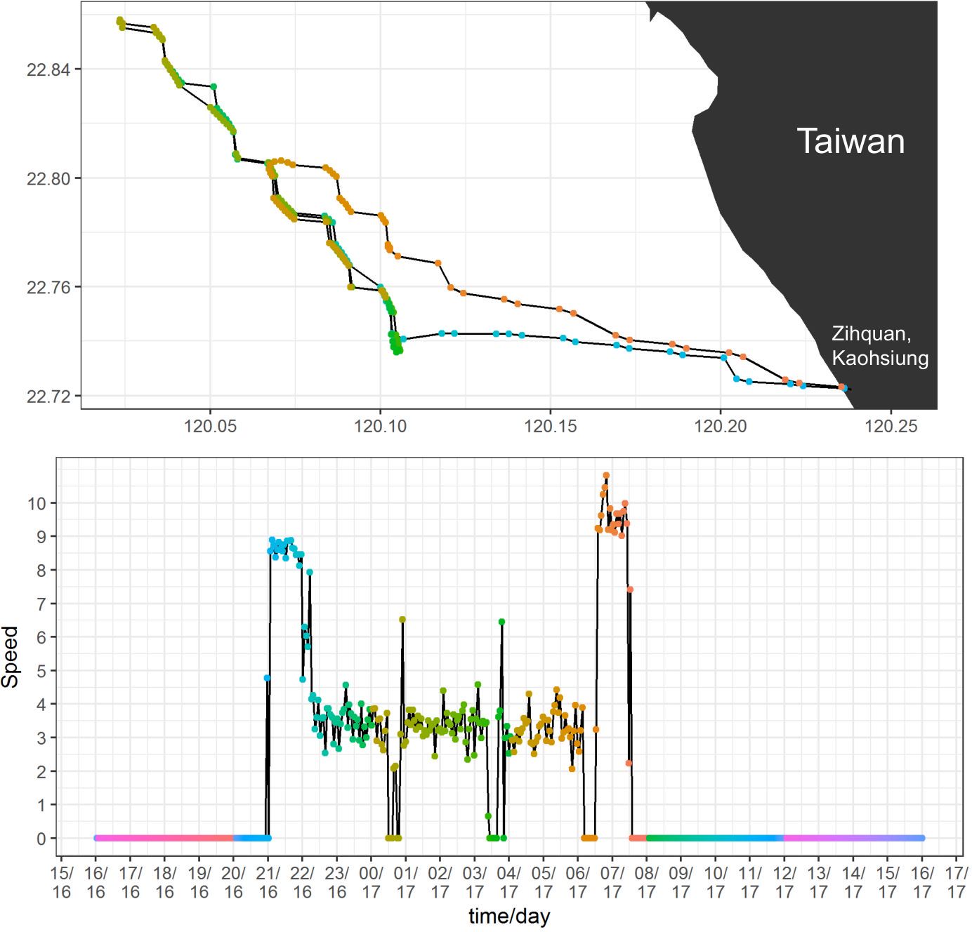
Figure 1 VDR position and vessel speed of a Taiwanese coastal trawler fishing for blackmouth croaker in southwestern Taiwan during January 16–17 of 2011. The upper panel indicates vessel tracks with latitude on the Y axis and longitude on the X axis, and the bottom panel indicates vessel speeds with time and date on the X axis and speed (knots) on the Y axis. The two panels include corresponding color dots to indicate which points on the map (top panel) correspond to which points in the speed time series (bottom panel). The colors rotate, and dots may overlap in the same position in the upper panel. More descriptions on the plots can be found in Supplementary Material.

Based on the work of Chang (2016) and interviews with fishermen, the following rules were established and applied to the VDR data to estimate fishing effort through an automated algorithm: (1) the VDR records that leaving from and later returning to the fishing port were marked as a trip. The number of VDR records between leave and return must be over 40 (about 2h). The VDR records located continuously in port were excluded. (2) The records with a speed of 2–5 knots for at least ten consecutive records (approximately 30 min) were considered as fishing. The short period of slow speed leaving and returning the port was considered as navigating. (3) The location in a resolution of 0.1° square that the vessel stayed longest during the fishing day was defined as the representative fishing location. (4) The records with speed > 5 knots were assumed to be navigating (e.g., transiting to fishing grounds).

The spatial distributions of VDR records identified as fishing according to rule (2) are illustrated in Figure 2. It is important to note that the VDR record distribution may cover a larger area than the CPUE distribution used for standardization analyses, as only one location in a trip was chosen to represent fishing according to rule (3).

Figure 2

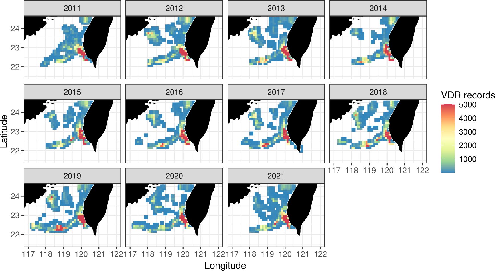
Figure 2 Spatial distribution of VDR records (considered as fishing) of the 29 sample vessels for this study from 2011 to 2021.

Following the outlined procedures, a comprehensive dataset of trip records was collected from the sampled vessels. Multiple sets were deployed during each trip, as illustrated in Figure 1. However, the fishing hours per trip exhibited variability based on fishing conditions and weather. Therefore, fishing effort was calculated as fishing hours. Subsequently, the trip-basis effort data (measured in fishing hours) were integrated with the corresponding market landing data of the trip for the sample vessels, to construct a trip-basis logbook-like data with time and location information for the calculation of nominal CPUE (kg per hour). On average, these sample vessels undertook approximately 1,887 trips with 3.5 mt of blackmouth annually, each spanning an average of 5.3 fishing hours per trip (excluding transition time). Since the multispecies feature of the trawl fishery and the relatively low abundance of blackmouth stock, about 60% of the trips contained zero blackmouth catch.

2.3 CPUE standardization

2.3.1 Key effects considered

2.3.1.1 Environmental effect

The spatial distribution of marine fishes is strongly influenced by environmental factors. The studied region encompasses cold water from the China Coastal Current and warm water from the Kuroshio Branch Current in different seasons, so examining the environmental effect should be necessary. Blackmouth is distributed in a depth of 40 m–200 m (Shao, 2023). Hydrological data including sea temperature at depth of 109 m (tem109), salinity at depth of 109 m (sal109), density ocean mixed layer thickness (mlt), chlorophyll (chl), and seafloor potential temperature (sft) were collected from the Copernicus Marine Environment Monitoring Service (CMEMS) (https://resources.marine.copernicus.eu/products), for the region ranging from 117°E to 121°E and 21°N to 24°N (Figure 2). The environmental data were obtained from CMEMS Global Ocean Physics Reanalysis (https://doi.org/10.48670/moi-00021) for 2000–2019 and from the Operational Mercator global ocean analysis and forecast system (https://doi.org/10.48670/moi-00016) for 2020–2021. These data were cross-checked with similar datasets from the Ocean Data Bank that were sponsored by the National Science and Technology Council, Taiwan, with higher resolution around Taiwan but a shorter time period (2000–2018) (http://www.odb.ntu.edu.tw/odb-services/). While there were differences between the two datasets in absolute values, the trends were basically similar.

Temperature and salinity data exhibit variations at different depths, which can complicate the analysis process. To ensure a standardized analysis, a fixed depth of approximately 109 m was chosen. This depth corresponds to the estimated habitat water depth of the blackmouth croaker (Shao, 2023). Fixing the depth at a specific level allows for consistent comparisons and interpretations of temperature and salinity data across different sampling points, reducing the influence of depth-related variations in the analysis.

Considering the small geographic size of the studied area and small within-month variation of the environmental data observed, these remote-sensing environmental data were computed as monthly averages on a spatial resolution of 0.1° to be consistent with the spatial resolution of the fishery data, using R Statistical Software (v4.2.2; R Core Team, 2021).

2.3.1.2 Targeting effect

Many fisheries catch multiple species simultaneously. When fishers specifically target a species during a fishing trip, they may employ fishing operations or techniques that are not optimized for catching other species (Okamura et al., 2018). This fishing strategy (i.e., targeting) may affect the catchability and the representativeness of CPUE as the abundance index and thus requires to be addressed in the standardization process (Maunder and Punt, 2004; Chang et al., 2011, Chang et al., 2019).

Two methods were used to generate targeting covariates. The first one was the k-means clustering method, which is a non-hierarchical clustering technique (Tan et al., 2006). The desired number of clusters (k) was chosen according to the “elbow method” (Kassambara, 2017) with scree plots (Chang et al., 2019). The species composition of the catch data was partitioned into k groups using this method, and the group ID was subsequently utilized as a categorical variable in the standardization model.

Winker et al. (2013), Winker et al. (2014) suggested a different approach to address the targeting effect in CPUE standardization for multispecies fisheries by employing PCA to calculate continuous principal components (PCs) of catch composition. This study applied the same approach and used these PC scores, which were assigned to each CPUE record, as predictors (continuous variables) in the standardization model to account for changes in fishing tactics over time (i.e., shifts in target species). More information on the approach can be found in the cited works (Winker et al., 2013, 2014; Chang et al., 2019).

Taiwanese offshore trawl fishery in the southwestern region is a multispecies fishery that includes nearly 200 species. Major commercial species such as Loliginidae, Carangidae, Centrolophidae, Priacanthidae, Trichiuridae, and Sciaenidae (including blackmouth croaker and bighead croaker that were targeted simultaneously) were selected and grouped as the primary targets of the fishery, and the remaining fish species (approximately 150 species, including many valuable species to some trawlers) are categorized as the fish group of “others” fishes. Catches of the seven species groups were aggregated by trip and transformed to catch composition in percentage before applying PCA.

2.3.1.3 Spatial effect

Fishery-dependent CPUE data are often characterized by high heterogeneity in the spatial distribution of habitat quality and fishing effort (Hsu et al., 2022; Pourtois et al., 2022). Therefore, considering spatial factors in statistical models can compensate for the limitations of traditional analysis methods. The presence of spatial autocorrelation in fishing catch data can be assessed using the Moran’s I test, where a significant result indicates the presence of spatial effects (Cliff and Ord, 1981). Description of the computation of Global Moran’s I is provided in Supplementary Section 1.

2.3.2 Statistical models

This study adopts a two-stage procedure (delta procedure), which consists of a PCM and a ZPM to address the high probability of zero catch values in the fishery data (Lo et al., 1992; Chang et al., 2019). For the PCM, ln(CPUE) are modeled assuming a normal distribution, while the ZPM predicts the presence or absence of blackmouth using logistic regression. The standardized index was the product of these model-estimated components.

2.3.2.1 Delta-GLM and delta-GAM

GLM and GAM were used for the CPUE standardization. For the PCM, the GLM assumes that the expected value of a transformed response variable is a linear combination of exploratory variables (Guisan et al., 2002) (see Supplementary Section 1). The GLM of this study specifies the response variable to be the natural logarithm of blackmouth CPUE.

The GAM (Hastie and Tibshirani, 2017) (Supplementary Material) is a semi-parametric extension of GLM, with the underlying assumption that the response variable is related to smooth additive functions of the explanatory variables. GAM was used because of the concern that GLM cannot handle potentially nonlinear relationships between CPUE and PC covariates (Winker et al., 2013).

The covariates considered in the models included: year (2011–2021), quarter (Q1–Q4), targeting factor (k-means or PCs), environmental factor, spatial factor (0.1° × 0.1° grid cell), and vessel factor. Vessel factor, in terms of vessel identification (vessel ID), was considered because each fishing vessel has its own unique characteristics, experience, and fishing capability, in addition to vessel size, which can impact catchability and the representativeness of CPUE as a resource indicator. The factors of year, quarter, vessel size, and target factor of k-means were treated as categorical variables, and the rest were treated as continuous variables. The environmental and principal component variables were modeled as smoothers in the GAM.

Spatial factor was treated as a random effect for all standardization models. Vessel factor was treated as a fixed effect in some models and a random effect in others. All remaining factors were treated as fixed effects. Helser et al. (2004) recommended treating the vessel factor as a random effect as it allows the data from various vessels to be combined and a single continuous time series of biomass indices to be developed. When random effects were considered, the mixed-effect models (i.e., GLMM and GAMM) were used for the CPUE standardization (Su et al., 2008; Forrestal et al., 2019; Grüss et al., 2019). A list of all model structures, as specified in the input to R, was provided in the Supplementary Material.

The ZPM predicts the presence or absence of blackmouth using logistic regression in GLM or logistic regression additive model in GAM (Supplementary Material).

The GLM/GAMs (without random effects) and GLMM/GAMMs (with random effects) were constructed using R Statistical Software (v4.2.2; R Core Team, 2021) and the function of the mgcv (Wood and Wood, 2015) and gamm4 package (Wood et al., 2017).

2.3.2.2 Spatiotemporal model (VAST)

R package VAST (version 3.10.0) (https://github.com/James-Thorson-NOAA/VAST) developed by Thorson (2019) was applied in this study. By default, VAST is a delta-generalized linear mixed modeling (GLMM) framework that separately estimates the probability of encounter (ZPM) and the mean catch rate of positive catches (PCM) (Supplementary Material).

Both the spatial and spatiotemporal random effects are assumed to be correlated in space; specifically, we smooth the spatial random effect by assuming that residuals at nearby sites are more similar than those at remote sites. The correlation between the spatial and spatiotemporal residuals at two locations (s and s’) is assumed to decrease as the distance between them increases. This decrease in correlation is modeled using the Matérn function (Supplementary Material).

2.3.2.3 Nonlinear-featured VAST

By default, VAST assumes a linear effect for each covariate, but it might be enhanced to perform nonlinear features. GAM is suitable for handling potentially nonlinear relationships between CPUE and covariates (e.g., PCs) (Winker et al., 2013). We, therefore, utilize the outcomes from GAM and polynomial basis expansion to capture the nonlinear impact of environmental factors and PCs on CPUE. The model was arbitrarily termed as “VAST (nonlinear)” here, in contrast to “VAST (linear),” and can be expressed as:

$$\begin{array}{l}\mathit{\text{logit}}({\mathit{\text{p}}}_{\mathit{\text{i}}})={\mathit{\text{β}}}_{\mathbf{1}}({\mathit{\text{t}}}_{\mathit{\text{i}}})+{\mathit{\text{L}}}_{{\mathit{\text{ω}}}_{\mathbf{1}}}{\mathit{\text{ω}}}_{\mathbf{1}}({\mathit{\text{s}}}_{\mathit{\text{i}}})+{\mathit{\text{L}}}_{{\mathit{\text{ε}}}_{\mathbf{1}}}{\mathit{\text{ε}}}_{\mathbf{1}}({\mathit{\text{s}}}_{\mathit{\text{i}}},{\mathit{\text{t}}}_{\mathit{\text{i}}})+{\mathit{\text{L}}}_{{\mathit{\text{δ}}}_{\mathbf{1}}}{\mathit{\text{δ}}}_{\mathbf{1}}({\mathit{\text{v}}}_{\mathit{\text{i}}})\hfill \\ +{\displaystyle \sum _{\mathit{\text{p}}=\mathbf{1}}^{{\mathit{\text{n}}}_{\mathit{\text{p}}}}{\displaystyle \sum _{\mathit{\text{k}}=\mathbf{1}}^{{\mathit{\text{n}}}_{\mathit{\text{k}}}}{\mathit{\text{γ}}}_{\mathbf{1},\mathit{\text{k}}}(\mathit{\text{p}}){\mathit{\text{f}}}_{\mathbf{1},\mathit{\text{k}}}(\mathit{\text{X}}({\mathit{\text{s}}}_{\mathit{\text{i}}},{\mathit{\text{t}}}_{\mathit{\text{i}}},\mathit{\text{p}}))}}+{\displaystyle \sum _{\mathit{\text{j}}=\mathbf{1}}^{{\mathit{\text{n}}}_{\mathit{\text{j}}}}{\displaystyle \sum _{\mathit{\text{k}}=\mathbf{1}}^{{\mathit{\text{n}}}_{\mathit{\text{k}}}}{\mathit{\text{λ}}}_{\mathbf{1},\mathit{\text{k}}}(\mathit{\text{j}}){\mathit{\text{g}}}_{\mathbf{1},\mathit{\text{k}}}(\mathit{\text{Q}}(\mathit{\text{i}},\mathit{\text{j}}))}}\hfill \end{array}$$

and

$$\begin{array}{l}\mathit{\text{log}}({\mathit{\text{u}}}_{\mathit{\text{i}}})={\mathit{\text{β}}}_{\mathbf{2}}({\mathit{\text{t}}}_{\mathit{\text{i}}})+{\mathit{\text{L}}}_{{\mathit{\text{ω}}}_{\mathbf{2}}}{\mathit{\text{ω}}}_{\mathbf{2}}({\mathit{\text{s}}}_{\mathit{\text{i}}})+{\mathit{\text{L}}}_{{\mathit{\text{ε}}}_{\mathbf{2}}}{\mathit{\text{ε}}}_{\mathbf{2}}({\mathit{\text{s}}}_{\mathit{\text{i}}},{\mathit{\text{t}}}_{\mathit{\text{i}}})+{\mathit{\text{L}}}_{{\mathit{\text{δ}}}_{\mathbf{2}}}{\mathit{\text{δ}}}_{\mathbf{2}}({\mathit{\text{v}}}_{\mathit{\text{i}}})\hfill \\ +{\displaystyle \sum _{\mathit{\text{p}}=\mathbf{1}}^{{\mathit{\text{n}}}_{\mathit{\text{p}}}}{\displaystyle \sum _{\mathit{\text{k}}=\mathbf{1}}^{{\mathit{\text{n}}}_{\mathit{\text{k}}}}{\mathit{\text{γ}}}_{\mathbf{2},\mathit{\text{k}}}(\mathit{\text{p}}){\mathit{\text{f}}}_{\mathbf{2},\mathit{\text{k}}}(\mathit{\text{X}}({\mathit{\text{s}}}_{\mathit{\text{i}}},{\mathit{\text{t}}}_{\mathit{\text{i}}},\mathit{\text{p}}))}}+{\displaystyle \sum _{\mathit{\text{j}}=\mathbf{1}}^{{\mathit{\text{n}}}_{\mathit{\text{j}}}}{\displaystyle \sum _{\mathit{\text{k}}=\mathbf{1}}^{{\mathit{\text{n}}}_{\mathit{\text{k}}}}{\mathit{\text{λ}}}_{\mathbf{2},\mathit{\text{k}}}(\mathit{\text{j}}){\mathit{\text{g}}}_{\mathbf{2},\mathit{\text{k}}}(\mathit{\text{Q}}(\mathit{\text{i}},\mathit{\text{j}}))}}\hfill \end{array}$$

where β(t_i) is the intercept for year t_i, ω(s_i) denotes time-invariant spatial variations at location s_i, ε(s_i,t_i) denotes time-varying spatiotemporal variations at location s_i in year t_i, and δ(v_i) denotes the effect of vessel v_i on catchability and is normally distributed (δ_l(v_i)~N(0,1),l=1,2), L_ω and L_ε are the scaling coefficients of the spatial and spatiotemporal random effect distributions. In addition, the γ(p) is the p^th habitat covariate X(s_i,t_i,p) at location s_i in year t_i (i.e., the impact of environmental factors on observed blackmouth CPUE) and the λ(j) is the j^th catchability covariates Q(i,j) for observation i (i.e., the impact of target factor (k-means or PCs) on observed blackmouth CPUE and the quarter factor) (Thorson, 2019). The nonlinear features are denoted by f_1,p(·), f_2,p(·), g_1,j(·) and g_2,j(·), which are the results from a GAMM that uses a polynomial spline for the basis. R-codes of this approach are provided in the Supplementary Material.

Calculations of abundance indices for the statistical models are provided in Supplementary Material.

2.4 Models design and explanatory power evaluation

This study constructed a model structure with 15 model designs (M1–M15) to compare the influences of the three statistical models (GLM, GAM, and VAST) and the four key factors: environment factor (with or without), vessel factor (treated as fixed or random effect), spatial factor (with or without), and target factors (addressed by k-means or PCA methods) (Table 1). A flowchart showing the compositions of the models investigated is shown in Figure 3. Each model has a corresponding model to compare with; for example, M1 is to compare with M0 to see the effect of environmental factor, and M2 is to compare with M1 to see the effect of treatment of target factor using k-means versus PCA (the last column of Table 1). The study performed four sets of comparisons: the first set (S1) compared M1–M5 for environment factor and treatment of target factor. Including environment factor in the rest models, the second set (S2) compared M6–M7 for vessel factor and target factor, without consideration of spatial factor, and the third set (S3) compared M8–M11 for vessel factor and target factor under the consideration of spatial factor. With fixed vessel factor and PCA-treatment of target factor, the fourth set (S4) compared M12–M15 for statistical models. QQ plots of all the models are provided in Supplementary Material and suggested that they all conformed with the lognormal distribution assumption, affirming the appropriateness of the assumption regarding the error distribution for the CPUE standardization.

Table 1

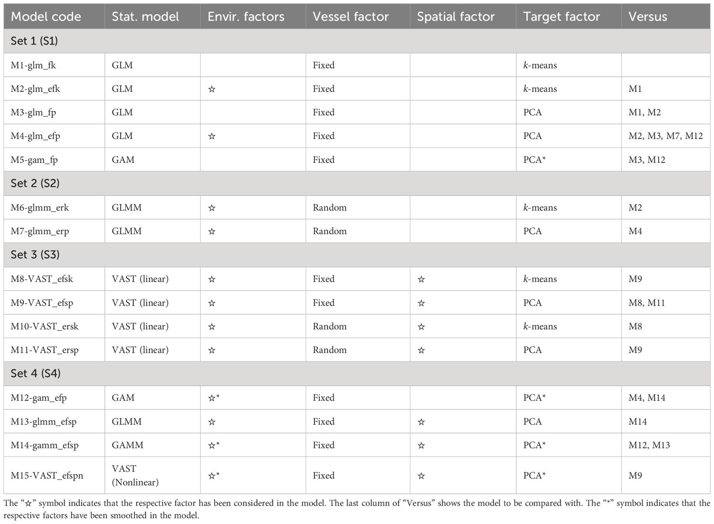
Table 1 The 15 CPUE standardization models designed in this study to compare the influences of three statistical models and four key factors.

Figure 3

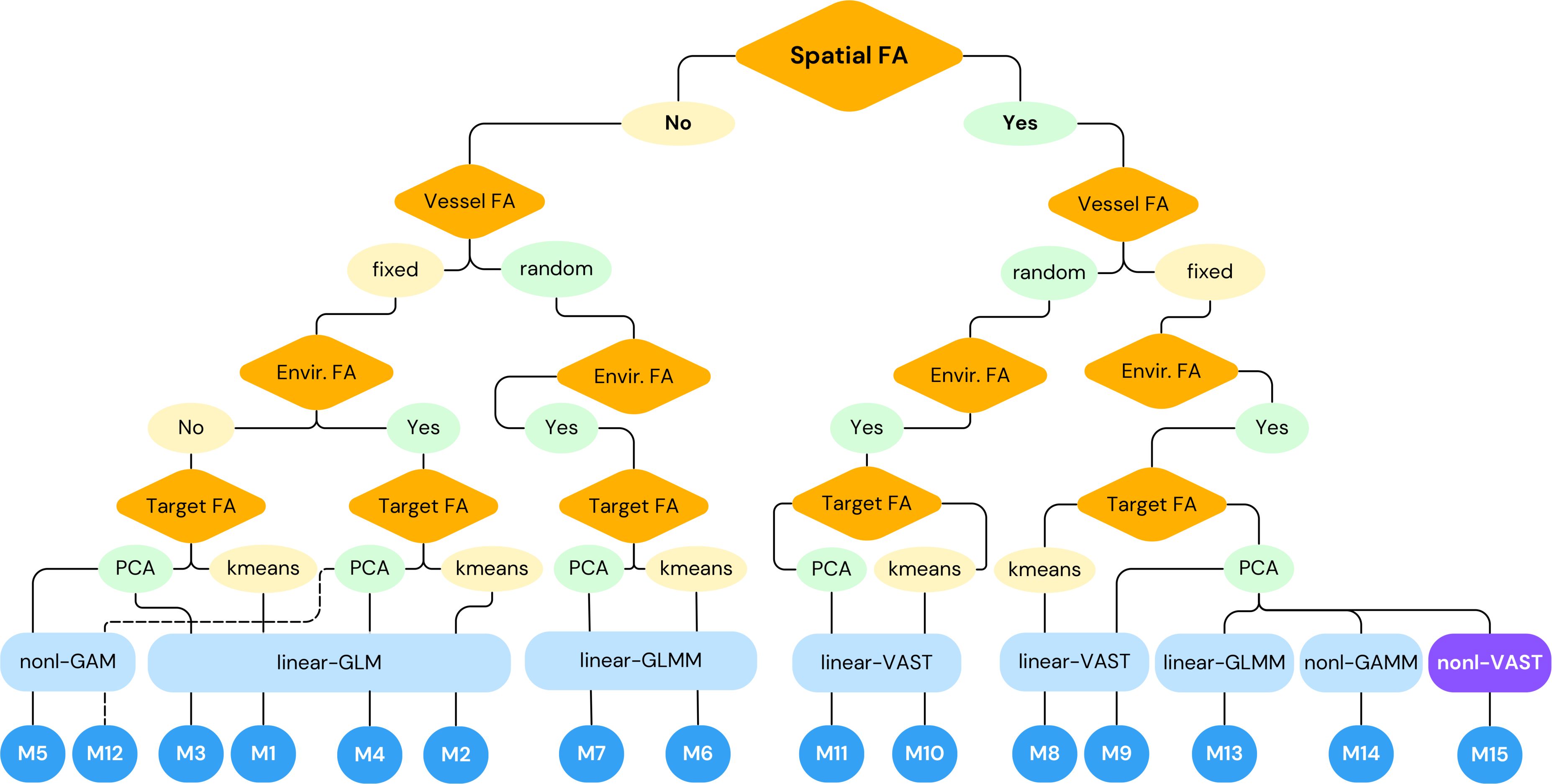
Figure 3 Flowchart showing compositions of the models investigated in this study. Orange diamonds are factors (FA), yellow and light green ovals are decisions to the factors, light blue squares are statistical models applied (the best model M15 using nonlinear VAST was marked in purple), and blue circles are model codes as shown in Table 1.

The study examined the predictive capability of two categories of methods introduced by Hinton and Maunder (2004) for CPUE model evaluation. The first category applied pseudo-R² (higher value preferred), a log-likelihood–based measurement representing the improvement in model likelihood over a null model (Faraway, 2016; Chang et al., 2019).

The second category was the cross-validation (CV) method. The study applied a stratified random sampling approach using year and vessel as strata in the fivefold CV procedure. After repeated 20 times, the CV-R² that determines the overall correlation between the actual and predicted value (Li et al., 2011; Chang et al., 2017; Zhang et al., 2023) was calculated and averaged. CV-R² was used to evaluate model’s EP.

Although the Akaike information criterion (AIC), falling into the second category, is also a valuable and widely employed tool for model comparison, it is crucial to recognize that its values are impacted by the sample size, because they are derived from a likelihood function. Therefore, as elucidated in Chang et al. (2019) and the citation, caution is warranted when comparing one-stage GLMs and two-stage delta-GLMs with different sample sizes using AIC. Additionally, specifying the variance parameters of the likelihood function in two-stage delta-GLM or delta-GAM cases is a complex undertaking. Therefore, this study used CV-R² when evaluating model EP.

3 Results

3.1 Fishing effort

Figure 1 provides an example of a VDR data track for effort estimation; an explanatory plot modified from Chang (2016) is provided in Supplementary Material. The 2011–2021 data obtained from the FA of Taiwan contains 29 vessels and 45,000 records in the study area. Using the procedures described in Section 2.1, about 43,530 trips with 210 tons of blackmouth catch and 230,809h of fishing effort were constructed from the data. Figure 2 shows the distribution of the fishing efforts, which were used for the following analyses.

3.2 CPUE standardizations

3.2.1 Targeting effect

Catch composition data were used for the targeting effect analyses, representing potential targeting strategies. For the k-means method, which minimizes the sum of squares from points to the cluster centers, there is no clear number of clusters suggested by the scree plot from the elbow method, but an ad hoc choice of five clusters could be a compromise option between smaller improvement of within-cluster sum of square and not too large number of clusters. Each of the clusters has different dominant species compositions (Figure 4), indicating five different types of target trips by the sample vessels: the dominant species of Cluster 1 is Sciaenidae, Cluster 2 Carangidae, Loliginidae, and “others” (other fishes), Cluster 3 Centrolophidae and “others,” Cluster 4 mainly “others,” and Cluster 5 Priacanthidae, Trichiuridae and “others.” Cluster 1 has the highest blackmouth catch composition, and the size of this cluster varied by year and was higher in 2011–12 and 2015. The cluster numbers were treated as categorical variables in the standardization model.

Figure 4

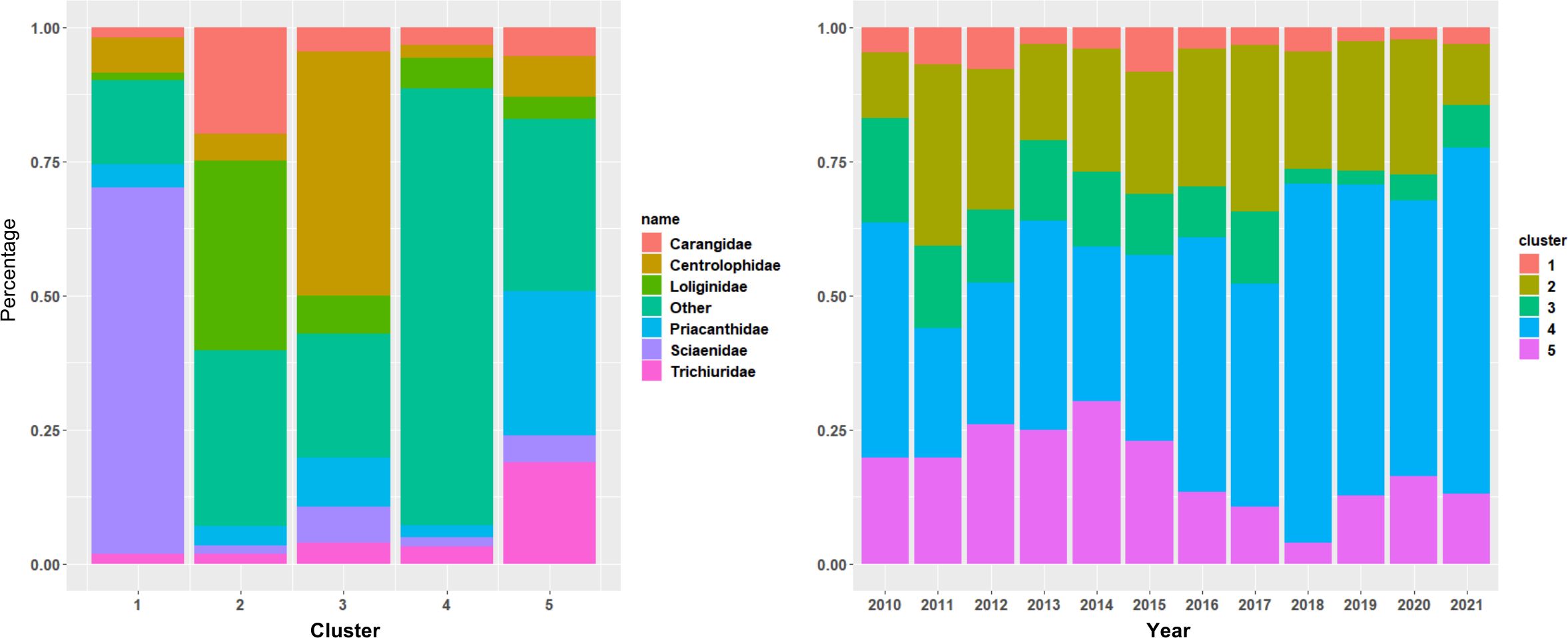
Figure 4 Species composition by cluster from k-means clustering method applied to market landing data from coastal trawlers fishing in the southwestern waters of Taiwan. Left panel: the species group composition by cluster; right panel: change of cluster membership through time.

Supplementary information on how the PCA results compare to the clustering is provided in the Supplementary Material.

For the PCA method, the scree plot shows that more than 70% of the total variance can be explained by the first four principal components. Figure 5 displays the weights of different species in the first four principal components. PC1 is dominated by “others” fishes, PC2 by Carangidae species, PC3 by Loliginidae species, and PC4 by Trichiuridae and Sciaenidae species. The correlation biplots expressing the loadings of the species composition on the PCs (Figure 6) suggested that, for example, PC2 has a strong positive correlation with both Carangidae and Loliginidae but a weak negative relationship with Sciaenidae. PC2 is the variable with the strongest (negative) effect; higher scores on PC2 indicate a considerable increase in the catch composition of Carangidae and Loliginidae but a relatively lower composition of Sciaenidae. Furthermore, PC4, with a slightly lower effect than PC2, demonstrates a strong negative correlation with the composition of Sciaenidae and a strong positive correlation with Trichiuridae. Higher scores on PC4 signify a substantial increase in the composition of Trichiuridae and a considerable decrease in the composition of Sciaenidae.

Figure 5

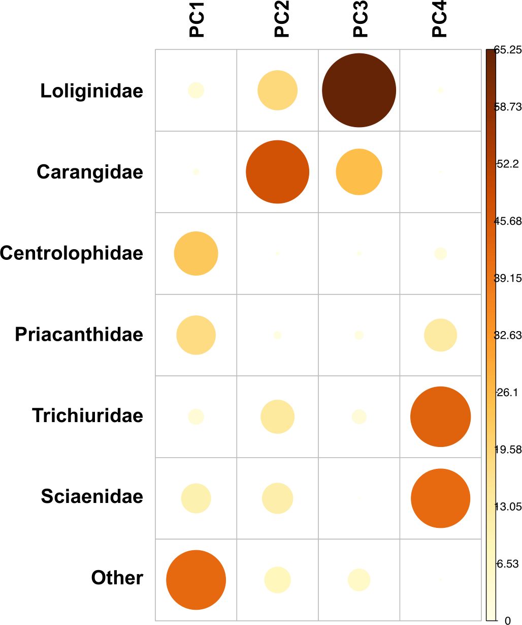
Figure 5 The weights of contributing species for each principle component (PC) of the PCA on the market landing data from coastal trawlers fishing in the southwestern waters of Taiwan. The size of the points represents the magnitude of the weights, with larger points indicating higher weights.

Figure 6

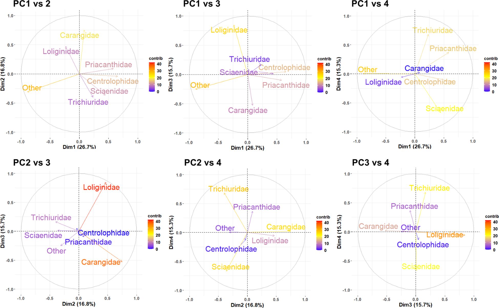
Figure 6 Correlation biplots showing the loadings of the fish species composition on the principle components. The color bar indicates the expected average contribution of a variable for two principal components.

3.2.2 Spatial effect

The Spatial Autocorrelation (Global Moran’s I test) tool was used to assess spatial autocorrelation by considering both the locations and response variables of features simultaneously. It examines whether the observed pattern of the features is clustered, dispersed, or random. The values of Moran’s I were statistically significant (I = 0.0047, P< 0.001) in this study, and the spatial factor was included in GLMM and GAMM to test the EPs of spatial and non-spatial models that will be presented in the followings.

In VAST, both the spatial and spatiotemporal random effects for a grid cell are assumed to come from the closest knot in space. This assumption simplifies the computational calculations involved in the model. All the spatiotemporal models successfully converged in the study, which was confirmed by the fact that the Hessian matrix was positively definite, and the maximum gradient component was smaller than 0.001. The spatiotemporal distribution of the predicted density of blackmouth showed a stable or slightly increasing pattern before 2016; thereafter, however, the density showed a continuous declining pattern, especially in the coastal areas of Taiwan and some offshore regions, with a rebound in 2018 mainly in the northern region of the coast (Figure 7, based on results of M15).

Figure 7

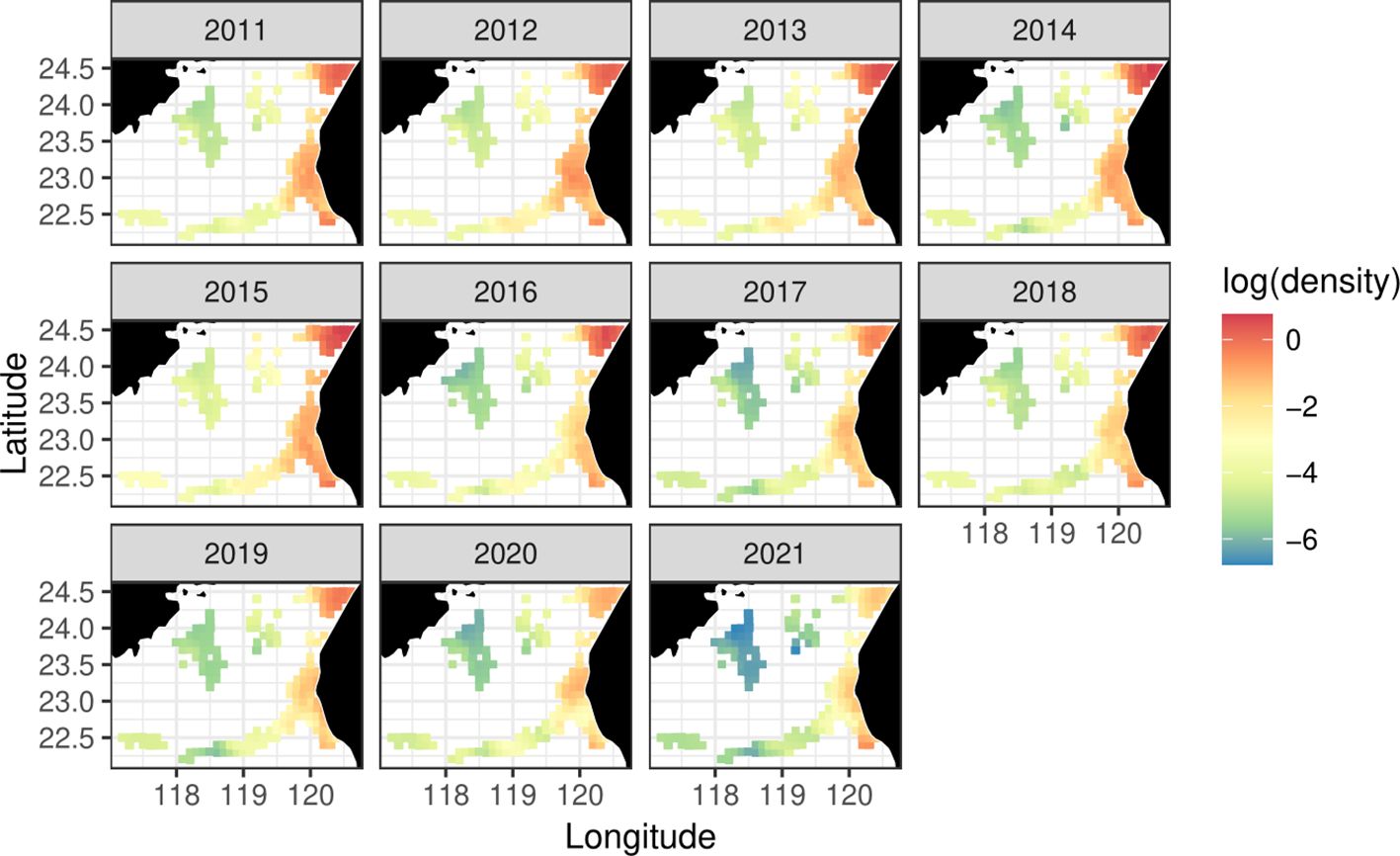
Figure 7 Spatiotemporal distributions of log-transformed blackmouth density in southwestern Taiwan from 2011 to 2021. The density was estimated from VAST (model M15), including those extrapolated over the unsampled area for some years.

3.3 Model explanatory power evaluation

Two R² (pseudo-R² and CV-R²) of the 15 models (M1–M15) are shown in Tables 2 (for model sets S1–S3) and Table 3 (for S4). The environmental effect was evaluated through S1 comparison under the consideration of vessel factor as a fixed effect: the R² between M2 (including environment factors) and M1 (without environment factors) are not much different. The same observation was noted for M3/M4 that used PCA for the target factor, compared to M1/M2 that used k-means. Another pair of tests (M5 and M12) using GAM instead of GLM showed that the model with environment factors (M12) has better EP (i.e., higher R²) than without (M5), although the differences were not substantial. The EP of M12 were much better than M2 and M4, which might suggest that the nonlinear features of environment factors could be better explained by the nonlinear GAM model.

Table 2

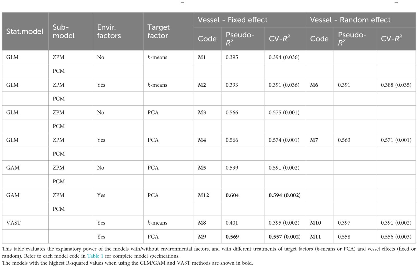
Table 2 Summary statistics of CPUE standardization models M1–M12 fitted to blackmouth croaker data off southwestern Taiwan during 2011–2021.

The effect of the method in addressing target factor was explored by comparing M1/M2 with M3/M4 and M8 with M9 when considering vessel factor as a fixed effect and by comparing M6 with M7 and M10 with M11 when considering vessel factor as a random effect (Table 2). All these comparisons suggested that the PCA method performed better than the k-means method.

The effect of the treatment of vessel factor was evaluated by comparing of M2 with M6, M4 with M7, M8 with M10, and M9 with M11 (Table 2). These comparisons suggested that models perform slightly better when the vessel factor is considered as a fixed effect instead of a random effect.

The spatial effect and EP of different statistical models were evaluated through comparisons with models of M4 and M12–14 that included environment factors, treated vessel factor as a fixed effect, and addressed target factor by PCA (Table 3). The results suggested that considering spatial random effect (delta-GLMM or delta-GAMM, M13–M14) resulted smaller R² than compared to those without (delta-GLM and delta-GAM, M4 and M12), and the M12 using GAM type model (delta-GAM) without consideration of spatial effect has the second-best EP (highest R²: pseudo-R² = 0.604 and CV-R² = 0.594).

Table 3

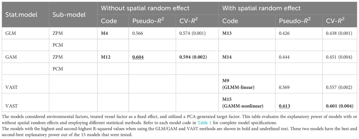
Table 3 Summary statistics of CPUE standardization models M4, M9, and M12–M15 fitted to blackmouth croaker data off southwestern Taiwan during 2011–2021.

The above comparisons using traditional GLM/GAM type statistical models showed that spatial effect might not be important in the standardization. However, when applying VAST and including spatial and spatiotemporal effects, the EP measures of M9 and M15 were much higher than those of M13 and M14, which applied GLM/GAM (linear and nonlinear) approaches. It might imply that spatial effect was important but needed a better approach to handle. The nonlinear-featured VAST (M15) demonstrated to have the best EP among all model designs (pseudo-R² = 0.613 and CV-R² = 0.601, Table 3).

Table 4 was created for explanatory purposes on the significance of the factors. Table 4 indicates that all the main effects were significantly different from zero at a significance level of α = 0.05 for M4 and M12, except for the chlorophyll factor that was not significant for the PCM sub-model of delta-GLM. Sea temperature and salinity at a depth of 109 m were excluded from PCM but were included and statistically significant in ZPM in the process of model selection. Figure 8 shows the estimates of fixed-effect factors of the year, quarter, and vessel from M12 (GAM), along with the smoothers for the PCA target factor and environment factor. The figure suggested that the highest CPUE occurred in the third and fourth quarters and that the variation among vessels is high. The effect of environmental factors seemed not very strong (Table 4) and without clear patterns (Figure 7). Most of the variation could be explained by the targeting effect, especially the PC1, PC2, and PC4 (Table 4): blackmouth CPUE has general positive (but nonlinear) correlation with PC1 (Figure 7) which was negatively correlated with “others” fishes (Figure 6) (i.e., higher PC1 value has lower “others” fishes composition and higher Sciaenidae composition), and was nonlinearly negative correlation with PC2 and PC4 (Figure 7), which was negatively correlated with Sciaenidae (Figure 6).

Table 4

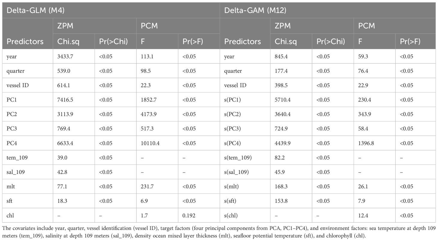
Table 4 Analysis of variance table for the model M4 (linear delta-GLM) and M12 (nonlinear delta-GAM).

Figure 8

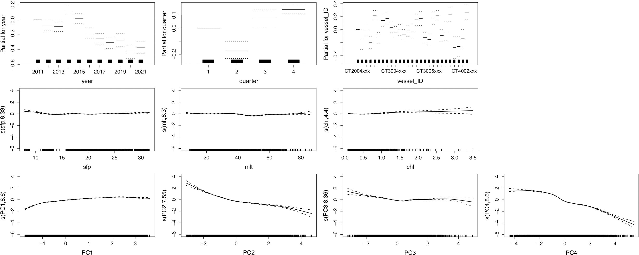
Figure 8 Impact of some of the main effects on the CPUE of blackmouth off southwestern Taiwan, from the results of model M12.

3.4 Trends of standardized indices

The standardized relative CPUE indices are shown for all the 15 models in Figure 9A and a subset of specifically selected eight models in Figure 9B. The general trend shows a decrease to 2013, an increase in 2014 and 2015 that was coincident with a weak to very strong El Niño event (Golden Gate Weather Services, 2023), and a continuous decline since then (although some models, especially the models used VAST, showed a noticeable increase in 2018 and then declined again). In the last year of the analysis in 2021, the indices show an increase to various degrees for all models using GLM- and GAM-type approaches but a continuous decline for models using the VAST approach except for models M8 and M10 that used k-means for targeting effect.

Figure 9

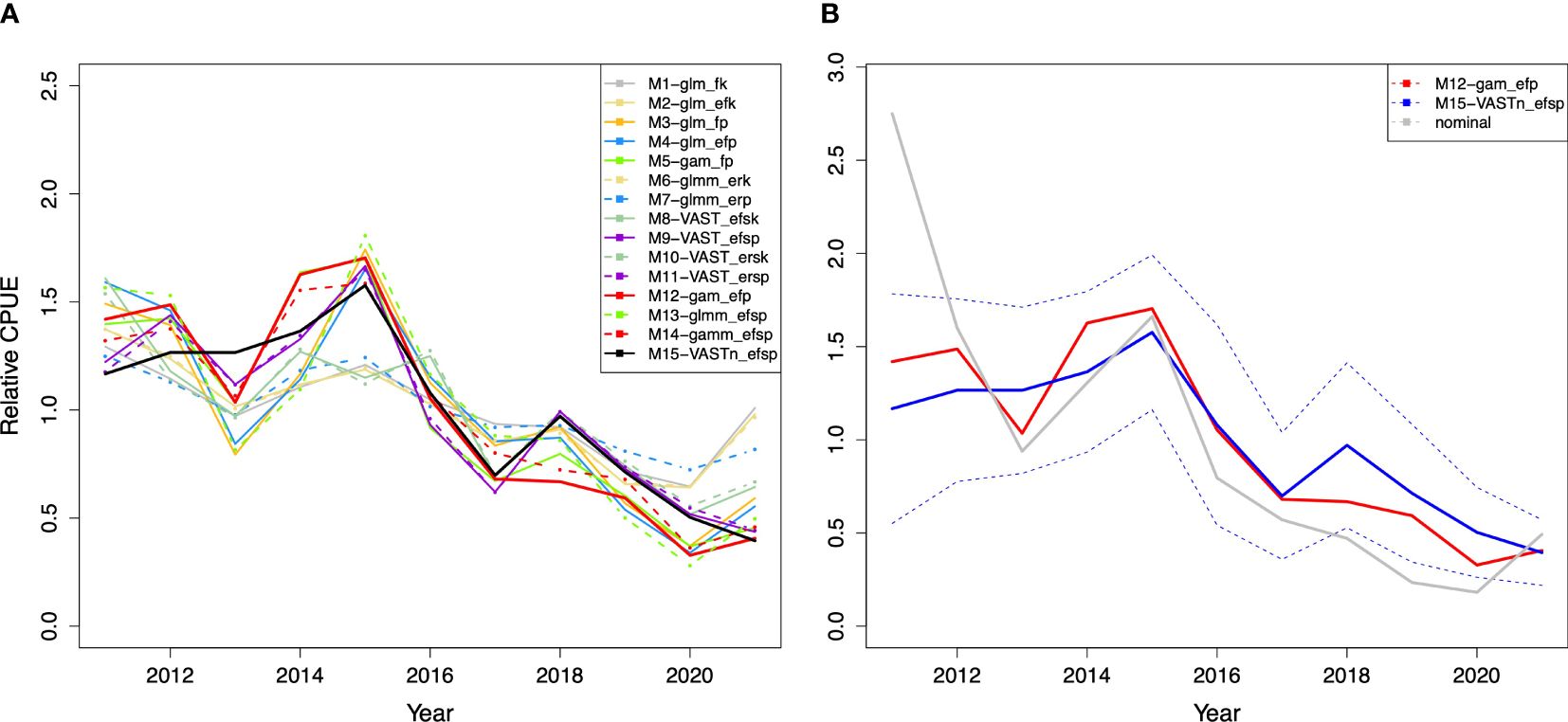
Figure 9 Relative CPUEs of all the 15 tested standardization models (A) and of the best two models (M15 and M12) with the nominal CPUE (B) for blackmouth croaker from southwestern Taiwan during 2011–2021. The dash lines are 95% confidence intervals for the M15.

For the specifically selected subset of the CPUE series (Figure 9B): (1) M8 and M9 employ different approaches to handle the target factor, with M8 utilizing k-means and M9 employing PCA, resulting in significant differences in the observed trends. M9 has higher EP than M8. (2) M9 and M11 differ in the way of treating vessel factors, and they are almost identical. (3) M5 and M12 differ in whether the environmental factor is considered, and the trends were basically similar with some years of variations. (4) M12 and M14 differ in whether a spatial factor is considered, and the results were very similar. (5) M4 and M12 differ in the statistical model used (GLM or GAM), and the indices were very different. Finally, (6) M9, M11, and M15 all used VAST but differ in linear or nonlinear treatment of nonlinear factors (environment and PCs). The index of M15 differs from the M9/M11 only in the beginning period and shows a slightly stronger decline in the last year. All these models exhibit different trends of indices from GLM/GAM type models. M12 and M15 utilized a nonlinear approach with the GAM and VAST methods to address nonlinear environmental factors, and exhibited higher EP compared to M4, M9, and M11, which employed methods featuring linear GLM and VAST.

4 Discussion

4.1 Nominal CPUE construction

Logbooks play a crucial role in providing essential catch and effort data for calculating the index of stock abundance. However, numerous coastal and small-scale fisheries are exempted from logbook submissions. In such cases, particularly for high-commercially valued species, which are more susceptible to intense exploitation, landing data, including date information and vessel identity, serves as a viable alternative to represent the “catch”. Additionally, auxiliary data such as VMS, CSRS, VDR, or the automatic identification system (AIS) can be employed to estimate fishing efforts through fishery-specific algorithms (Gerritsen and Lordan, 2011; Chang, 2014, Chang, 2016; Sonderblohm et al., 2014).

Although VMS data have been extensively utilized for scientific purposes, the associated installation and transmission costs are high, making them less feasible for small-scale coastal vessels with limited capital. CSRS has its application limitations, such as the special system requirements to identify fishing vessels from the port and the potential degradation of radar data quality by environmental effects (Chang, 2014).

AIS, introduced by the IMO to enhance maritime safety and prevent ship collisions, offers comparable data to VMS but with improved temporal resolution at a significantly lower cost and can be used to derive fishing efforts and inform fisheries management (Natale et al., 2015; James et al., 2018). This study conducted a preliminary investigation into the utilization of AIS from Taiwanese coastal fishing vessels for scientific purposes, revealing challenges such as the short data period (since the AIS was introduced to fishing vessels late), low data coverage (because installation and operation of AIS are not compulsive for small-scale coastal vessels), and difficulties in identifying fishing vessels (due to the absence of a cross-reference template for AIS databases and fisheries management systems). These challenges are likely prevalent in other coastal countries.

In contrast, the VDR system proves more manageable for the Taiwanese case. The IMO’s Maritime Safety Committee mandated passenger ships and large vessels to carry a standard VDR for accident investigations since 2000, with a 2006 amendment introducing a requirement for a simplified VDR (IMO, 2006). Recognizing the potential for fraud in fuel cost subsidies, the FA of Taiwan mandated the installation of simplified VDR in 2010 (Chang, 2016). This cost-reduced VDR, which records date, time, GPS position, speed, and direction of the vessel at 3-min intervals, not only addresses fraudulent activities but also provides data for scientific use at minimal additional cost. The affordability of installation and transmission makes it feasible for sample vessels to carry VDRs for independent research purposes. This study demonstrates the feasibility of using VDR data to construct nominal CPUE and derive an abundance index for declining fish stocks.

4.2 Key factors and statistical models

Confounding factors inherent in the nominal CPUE data need to be carefully addressed before the CPUE can represent the abundance. This study designed 15 models to examine the effect of targeting, vessel, and environmental and spatial factors and explore the best model specification for the blackmouth stock off southwestern Taiwan.

4.2.1 Targeting effect

Target tactics of the fishers are one of the most important factors influencing the CPUE for a multispecies fishery (Okamura et al., 2018). Of the two commonly used methods to address the target factor (Campbell et al., 2017), this study showed that the PCA approach offered significantly higher EP than the k-means approach in terms of CV-R² (CV-R² = 0.391 vs. 0.575, refer to Section 3.3 and Table 2), regardless of how other factors were treated (CV-R² = 0.391 vs. 0.575, refer to Section 3.3 and Table 2). Moreover, noticeable differences in relative CPUE trends were observed between the two approaches (Figure 9B, M8 vs. M9). This observation aligns with the findings by Chang et al. (2019) during their CPUE standardization research on dolphinfish stock. Although this difference might be driven by the additional flexibility implied by the model structure using PCA, the PCA procedure has been highlighted for its effectiveness in mitigating the impact of targeting on multispecies CPUE (Winker et al., 2014). It achieves this by avoiding the need to determine an optimal number of clusters with rather artificial boundaries, as well as allowing the combinations of different proportions of targeting tactics to be modeled as a continuum of all possible combinations (Winker et al., 2013).

4.2.2 Vessel effect

Vessel factor (estimated using individual vessel ID) combined the effects of vessel features and the skill/experiences of the skipper, which have been demonstrated to be a major influential variable in CPUE studies (Bentley et al., 2012; Chang et al., 2019; Hsu et al., 2022). The vessel features may include the size of the vessel, which is usually associated with fishing power and capacity of the vessel and is an important characteristic of trawl vessels. For the Taiwanese case, the first digit of the vessel ID represents the size of the vessel and, thus, vessel size has been considered in the factor. The study showed that treating it as a fixed effect has slightly better EP than as a random effect (Table 2), but the difference is small, and the trends of relative CPUE are similar (Figure 9B, M9 vs. M11). This should be expected as there is more flexibility to fit a covariate to a fixed effect than a random effect, which is (by definition) constrained to be normally distributed with an estimated variance. The lack of difference in the indices may simply point out the fact that the vessel with effects that were shrunk (in the mixed framework) must not have represented a high number of records.

Vessel factor is statistically significant in model M12 (the second-best model in Table 4), although the F value is comparatively small. The coefficient of variation (cv) of the average blackmouth landings among the vessels was 60.2%, showing a high variation among vessels. Also, removing the vessel factor from M12 produced R² = 0.576, about 3% decline from the original M12, suggesting that the vessel factor was influential in the standardization.

4.2.3 Environmental effect

Environmental factors are supposed to have an impact on the CPUE of demersal species (Kempf et al., 2022). The three pairs of model comparisons (Table 2) suggested that including environment factors performed slightly better than without when using GAM type model (M5 and M12), and on the contrary, performed equally or even slightly worse than without ones when using GLM type model (M1–M4). This suggested that the importance of environmental factors for this study was not high, although two or three of the studied factors showed statistical significance (Table 4). This was speculated owing to the small size, hence less variation, of the studied area (Figure 2). Both the temperature (cv = 5.6%) and salinity (cv = 0.3%) factors were not significant just because of their small variation in this area.

4.2.4 Spatial effect

Spatial factor, the significance of which was tested using Moran’s I, was included as independent and identically distributed random effect in the mixed model analyses (GLMM and GAMM) or directly addressed using the spatiotemporal VAST model as a spatially autocorrelated random effect. The comparison of model EP (Table 3) suggested that including spatial factor did not perform better than those without, and the trends were very similar (Figure 9B, M12 vs. M14). Fish density distributed separately in four regions (Figure 7), and each region featured with different target species (in clockwise): (1) coastal region off Taiwan in the southeastern, targeting Sciaenidae, Priacanthidae, Trichiuridae, Centrolophidae in the southern part of this region, and Sciaenidae, Loliginidae, and “others” in the northern part; (2) South China Sea Slope in the south targeting “others”; (3) Xiapeng Depression in the northwestern targeting Loliginidae; and (4) Chang-Yuen Ridge in the northeastern targeting “others” and some Loliginidae. This suggested that the spatial effect might have largely been explained by the targeting effect in GLM/GAM type models (e.g., high F values for PC1–PC4 in Table 4).

There might be an issue with confounding among spatial, targeting, and environmental effects in the data analysis. It is concerning if the confounding did occur, because the spatial effect, unlike the targeting effect, should not be standardized out of the index, as it reflects true abundance. If the model is unable to distinguish the spatial effect from the targeting effect, it raises questions about the reliability of the standardized index. However, addressing confounding between abundance and catchability covariates is a complex challenge in CPUE standardization.

The spatial area depicted in Figure 2 exhibits some data coverage gaps. Since there is no published study defining the full range of the blackmouth croaker’s habitat and the southwestern region is regarded as a single stock (Hwang and Chen, 1984), this research encompassed the vessels’ entire distribution area as its study area. The reasons behind these data gaps are unclear, and the representativeness of the predictions in these sparsely covered regions remains uncertain. However, a significant data gap in the central section of Figure 7 could be linked to the presence of the Penghu Archipelago and Taiwan Bank.

When delineating the study area for CPUE analysis, it is important to consider the peripheral regions of the fishery that are rarely fished. It is uncertain whether these areas are unfished due to low CPUE or other reasons. Including such regions in the modeling process will introduce additional uncertainty since estimating abundance in these areas will rely on limited data (Hoyle et al., 2024). One approach to mitigate this concern is to confine the spatial scope to a “core” fishery, comprising the regions where the majority of the catch is obtained (Campbell, 2015; Hoyle et al., 2024).

The significance of spatial factors’ interpretation could vary depending on the statistical model employed. When incorporating spatial effects, the EP measures of M9 with VAST surpassed those of M13 (GLMM) and M14 (GAMM) (Table 3), implying that the additional flexibility provided by the Gaussian Markov Random Field in VAST allows for a better representation of spatial effects than a traditional random effect structure. Introducing a new model design (M15) that enables VAST to handle nonlinear features like M12 resulted in even higher EP compared to M12 without spatial effects. This suggests that spatial effects played an important role in standardization, with VAST showcasing their importance more effectively than GLM/GAM models, as indicated above.

Spatial effects are able to smooth the effect of multiple unaccounted drivers and can be modeled using geostatistics (INLA) and 2D smoothing splines of GAM (Paradinas et al., 2023). Modeling spatial effects in continuous space is one of the key appeals of the GAM approach for CPUE standardization (Table 2 of Hoyle et al., 2024). However, as indicated in Section 2.3.2.1, spatial factor was treated as a random effect for all analyses of this study. Exploring models where spatial factors are considered as a continuous 2-D surface may add complexity to the model investigation structure (Figure 3) but holds promise for future investigations.

4.2.5 Statistical models

Three types of statistical models were tested in the study. The models used nonlinear-featured GAM (or GAMM) all have better EP over linear-featured GLM (GLMM) and VAST (GLMM-based) (Tables 2 and 3). This was because the targeting effect is the most influential factor in this study (Table 4), and this factor was better represented by the nonlinear predictors allowed by the GAM.

The advantages of VAST have been successfully demonstrated in many CPUE standardization studies on pelagic and demersal species with spatiotemporal considerations (Grüss et al., 2019; Xu et al., 2019; Hsu et al., 2022; Kawauchi et al., 2023). The advantages, however, did not manifest in this study if using the default linear feature of the model (M9), as the VAST has a limited ability to include nonlinear relationships beyond general quadratic ones compared to GAMs or boosted regression trees (Brodie et al., 2020). This study designed a nonlinear-featured VAST, expanding the approach to include a nonlinear feature (M15) by taking advantage of the inputs from GAM to deal with nonlinear-featured environmental factors and PCs. The result has demonstrated substantial improvement in its predictive EP and, thus, was suggested to be applied to situations with nonlinear covariates.

One key advantage of spatiotemporal models such as VAST is that they allow a straightforward computation of “predict-then-aggregate” indices of relative abundance (sensu Hoyle et al., 2024). Since VAST imputes fish density in unsampled locations informed by a distance-based covariance function, the index can be computed from the entire spatial domain at each time step. It uses the area-weighting approach to compute the index of relative abundance. Providing interpolation of fish density distribution across the years (Figure 7) can also facilitate the interpretation of the spatiotemporal change of fish abundance. In comparison, traditional approaches to derive the index based on the year-effect only do not account for spatiotemporal variation in fish density over the entire spatial domain. Since fishing locations usually change over time, the index computed from the traditional year-effect approach may not be representative of the whole population, and, consequently, be proportional to the abundance of the whole population (Maunder et al., 2020).

The main finding from the model comparison exercise revealed that the model configurations with the highest EP, whether related to vessels, targets, or spatial aspects, tended to be the most complex ones. This outcome is not surprising considering the multifaceted nature of the fisheries system, which is influenced by a wide range of factors such as biology, economics, and the environment. As such, it is imperative to consider the nonlinear relationships that arise from these complex drivers when modeling such diverse systems (Glaser et al., 2014).

4.3 Abundance index

This study utilized two R² as EP metrics. However, it is crucial to emphasize that a higher R² do not necessarily equate to a more accurate index of relative abundance. The index of relative abundance, a pivotal input for stock assessment models, directly reflects changes in population abundance over time (Francis, 2011). The primary aim of CPUE standardization is to mitigate the influence of all factors except fish density on CPUE, ensuring that the standardized index of relative abundance approximates population abundance (MaunderTan and Punt, 2004). While a higher R² suggests a better fit and more accurate predictions for nominal CPUE data, they do not confirm whether the model accurately identifies and addresses other factors impacting catchability. Therefore, a careful consideration of the history of the fishery and the stock (e.g., in terms of fleet dynamics, possible changes in fishing gear configurations, economic incentives, shifts in species distribution) is required when selecting the best models to use for CPUE standardization.

The abundance indices derived from the best model (M15) and the second-best model (M12) both exhibited a general declining trend for the southwestern blackmouth stock. This marks the first abundance index developed for demersal fish species in the region. Limited academic studies on the stock status of fish resources in the region exist in the literature due to a scarcity of catch and effort data (Liao et al., 2019). Although abundance indices for other demersal fish species are unavailable, their landings indicate a similar declining trend, suggesting a broad degradation of fisheries resources in the region (based on fisheries statistical yearbooks, Fisheries Agency, 2022; Shao, 2023). Indirect methods, such as trophic models (Liu et al., 2009) or fishermen surveys (Liao et al., 2019), along with numerous gray literature sources, caution that overfishing has occurred to Taiwanese coastal blackmouth resources due to the overcapacity of fishing vessels and illegal fishing (Chang et al., 2010; Liao et al., 2019). Comparisons of growth parameters over a decade also imply high fishing pressures on blackmouth, resulting in elevated growth coefficients and smaller asymptotic lengths (Huang et al., 2022).

In addition to overfishing, environmental pollution is asserted to contribute to the degradation of the fishery environment in the region. Repeated pollution events in rivers flowing into the area have been documented for years without complete remediation (Liu et al., 2015; Wang et al., 2021; Liang et al., 2024). However, further studies are required to establish the impact of contaminations on fisheries resources.

5 Conclusions

Indices of relative abundance are one of the most essential data for stock assessments and consequent management advice. For data-limited small-scale coastal fisheries that are exempted from logbook submission, the abundance indices can be established through proper standardization on vessel-specific landing data and trip-based fishing effort estimated from geo-referenced position data.

This study utilized unique data sourcing from VDRs to estimate fishing effort, in combination with landing data to estimate the CPUE data for the blackmouth croaker in southwestern Taiwan (Figure 2), which demonstrated the potential application in global data-limited fisheries. The study also assessed alternative approaches for predictors of fishery targeting practices to condition effort for producing more accurate metrics of relative abundance. Fifteen models were designed for CPUE standardization, employing three statistical approaches. Model comparisons were conducted to scrutinize the impacts and treatments of targeting, vessel, environmental, and spatial factors. The results indicated that, in this multispecies fishery, the target factor explained the most variability in the observed catch rates, recommending the utilization of the PCA approach to address the target effect. It was advised to consider the vessel factor in the standardization process, either as a fixed effect with consistent specifications of sample vessels over years, or as a random effect following recommendations from Bentley et al. (2012) and Hsu et al. (2022). The inclusion of environmental factors did not notably enhance model EP, potentially due to the limited fishing area in this study. However, for fisheries with a broader spatial range, this factor should still be thoroughly examined. Because of the nonlinear feature of the PCA approach and environment data, GAM performed better than the linear-based models. However, with the expansion of VAST to include nonlinear features, the model surpassed GLM/GAM-type models in handling spatial random effects.

The best model (Model M15) exhibited a consistent declining trend in CPUE since 2015, with a brief rebound in 2018 (Figure 9B). The second-best model (M12) displayed a similarly sharp decline since 2015 but diverged in 2021. Despite this variation, the overall declining trend across all models signals the potential decline of the blackmouth stock, prompting the consideration of further management measures.

Data availability statement

The raw data supporting the conclusions of this article contains vessel’s identity and their confidential data of fishing locations and catches. It will be made available by the authors to qualified researchers under conditions. Requests to access these datasets should be directed to SC, skchang@faculty.nsysu.edu.tw.

Author contributions

TY: Formal analysis, Methodology, Software, Visualization, Writing – original draft. HX: Writing – review & editing. BL: Data curation, Software, Writing – review & editing. SC: Conceptualization, Funding acquisition, Resources, Supervision, Writing – original draft, Writing – review & editing.

Funding

The author(s) declare financial support was received for the research, authorship, and/or publication of this article. This research was funded by the National Science and Technology Council, Taiwan, grant number: MOST 110-2611-M-110-012 and MOST 111-2611-M-110-002.

Acknowledgments

The authors wish to express their appreciation to Shu-Chiang Huang, a PhD candidate at NSYSU, for her meticulous efforts in analyzing market data, and to Jhen Hsu, a PhD candidate at NTU, for her valuable insights into model analysis. We are also grateful to the Fisheries Agency of the Ministry of Agriculture for supplying the VDR data. Furthermore, our gratitude extends to the three Reviewers and the Editor for their insightful comments.

Conflict of interest

The authors declare that the research was conducted in the absence of any commercial or financial relationships that could be construed as a potential conflict of interest.

Publisher’s note

All claims expressed in this article are solely those of the authors and do not necessarily represent those of their affiliated organizations, or those of the publisher, the editors and the reviewers. Any product that may be evaluated in this article, or claim that may be made by its manufacturer, is not guaranteed or endorsed by the publisher.

Supplementary material

The Supplementary Material for this article can be found online at: https://www.frontiersin.org/articles/10.3389/fmars.2024.1344181/full#supplementary-material

References

Afonso-Dias M., Simões J., Pinto C. (2004). A dedicated GIS to estimate and map fishing effort and landings for the Portuguese crustacean trawl fleet. GISspatial Anal. Fish. Aquat. Sci. 2, 323–340.

Google Scholar

Bastardie F., Nielsen J. R., Ulrich C., Egekvist J., Degel H. (2010). Detailed mapping of fishing effort and landings by coupling fishing logbooks with satellite-recorded vessel geo-location. Fish. Res. 106, 41–53. doi: 10.1016/j.fishres.2010.06.016

CrossRef Full Text | Google Scholar

Bentley N., Kendrick T. H., Starr P. J., Breen P. A. (2012). Influence plots and metrics: tools for better understanding fisheries catch-per-unit-effort standardizations. ICES J. Mar. Sci. 69, 84–88. doi: 10.1093/icesjms/fsr174

CrossRef Full Text | Google Scholar

Bhattacharjee S. (2019) Voyage Data Recorder on a Ship Explained (Mar. Insight). Available online at: https://www.marineinsight.com/guidelines/voyage-data-recorder-on-a-ship-explained/ (Accessed February 17, 2024).

Google Scholar

Booth A. J. (2000). Incorporating the spatial component of fisheries data into stock assessment models. ICES J. Mar. Sci. 57, 858–865. doi: 10.1006/jmsc.2000.0816

CrossRef Full Text | Google Scholar

Brodie S. J., Thorson J. T., Carroll G., Hazen E. L., Bograd S., Haltuch M. A., et al. (2020). Trade-offs in covariate selection for species distribution models: a methodological comparison. Ecography 43, 11–24. doi: 10.1111/ecog.04707

CrossRef Full Text | Google Scholar

Campbell R. A. (2015). Constructing stock abundance indices from catch and effort data: Some nuts and bolts. Fish. Res. 161, 109–130. doi: 10.1016/j.fishres.2014.07.004

CrossRef Full Text | Google Scholar

Campbell R., Zhou S., Hoyle S., Hillary R., Auld S. (2017). Developing innovative approaches to improve CPUE standardisation for Australia’s multispecies pelagic longline fisheries (Canberra, Australia: Fisheries Research and Development Corporation (Australia).

Google Scholar

Chang S.-K. (2014). Constructing logbook-like statistics for coastal fisheries using coastal surveillance radar and fish market data. Mar. Policy 43, 338–346. doi: 10.1016/j.marpol.2013.07.003

CrossRef Full Text | Google Scholar

Chang S.-K. (2016). From subsidy evaluation to effort estimation: Advancing the function of voyage data recorders for offshore trawl fishery management. Mar. Policy 74, 99–107. doi: 10.1016/j.marpol.2016.09.017

CrossRef Full Text | Google Scholar

Chang S.-K., Hoyle S., Liu H.-I. (2011). Catch rate standardization for yellowfin tuna (Thunnus albacares) in Taiwan’s distant-water longline fishery in the Western and Central Pacific Ocean, with consideration of target change. Fish. Res. 107, 210–220. doi: 10.1016/j.fishres.2010.11.004

CrossRef Full Text | Google Scholar

Chang S.-K., Liu H.-I., Fukuda H., Maunder M. N. (2017). Data reconstruction can improve abundance index estimation: An example using Taiwanese longline data for Pacific bluefin tuna. PloS One 12, e0185784. doi: 10.1371/journal.pone.0185784

PubMed Abstract | CrossRef Full Text | Google Scholar

Chang S.-K., Liu K.-Y., Song Y.-H. (2010). Distant water fisheries development and vessel monitoring system implementation in Taiwan-History and driving forces. Mar. Policy 34, 541–548. doi: 10.1016/j.marpol.2009.11.001

CrossRef Full Text | Google Scholar

Chang S.-K., Yuan T.-L., Wang S.-P., Chang Y.-J., DiNardo G. (2019). Deriving a statistically reliable abundance index from landings data: An application to the Taiwanese coastal dolphinfish fishery with a multispecies feature. Trans. Am. Fish. Soc 148, 106–122. doi: 10.1002/tafs.10125

CrossRef Full Text | Google Scholar

Cliff A. D., Ord J. K. (1981). Spatial processes: models & applications. London: Pion.

Google Scholar

Duarte C. M., Agusti S., Barbier E., Britten G. L., Castilla J. C., Gattuso J.-P., et al. (2020). Rebuilding marine life. Nature 580, 39–51. doi: 10.1038/s41586-020-2146-7

PubMed Abstract | CrossRef Full Text | Google Scholar

Ducharme-Barth N. D., Shertzer K. W., Ahrens R. N. (2018). Indices of abundance in the Gulf of Mexico reef fish complex: A comparative approach using spatial data from vessel monitoring systems. Fish. Res. 198, 1–13. doi: 10.1016/j.fishres.2017.10.020

CrossRef Full Text | Google Scholar

FAO. (2023). The CWP Handbook of Fishery Statistical Standards. Catch and Landings. CWP Data Collection (Rome: FAO Fisheries and Aquaculture Department). Available online at: https://www.fao.org/cwp-on-fishery-statistics/handbook/capture-fisheries-statistics/catch-and-landings/en/ (Accessed September 15, 2023).

Google Scholar

Faraway J. J. (2016). Extending the linear model with R: generalized linear, mixed effects and nonparametric regression models, Second Edition (New York, USA: CRC press/Chapman & Hall). doi: 10.1201/9781315382722

CrossRef Full Text | Google Scholar

Fisheries Agency (2022). Fisheries Statistical Yearbook - Taiwan, Kinmen and Matsu Area 2021 (Taipei: Fisheries Agency, Ministry of Agriculture).

Google Scholar

Forrestal F. C., Schirripa M., Goodyear C. P., Arrizabalaga H., Babcock E. A., Coelho R., et al. (2019). Testing robustness of CPUE standardization and inclusion of environmental variables with simulated longline catch datasets. Fish. Res. 210, 1–13. doi: 10.1016/j.fishres.2018.09.025

CrossRef Full Text | Google Scholar

Francis R. I. C. C. (2011). Data weighting in statistical fisheries stock assessment models. Can. J. Fish. Aquat. Sci. 68, 1124–1138. doi: 10.1139/f2011-025

CrossRef Full Text | Google Scholar

Gerritsen H., Lordan C. (2011). Integrating vessel monitoring systems (VMS) data with daily catch data from logbooks to explore the spatial distribution of catch and effort at high resolution. ICES J. Mar. Sci. 68, 245–252. doi: 10.1093/icesjms/fsq137

CrossRef Full Text | Google Scholar

Glaser S. M., Fogarty M. J., Liu H., Altman I., Hsieh C.-H., Kaufman L., et al. (2014). Complex dynamics may limit prediction in marine fisheries. Fish Fish. 15, 616–633. doi: 10.1111/faf.12037

CrossRef Full Text | Google Scholar

Golden Gate Weather Services. (2023). El Niño and La Niña Years and Intensities. Available online at: https://ggweather.com/enso/oni.htm.

Google Scholar

Greenstreet S. P., Fraser H. M., Piet G. J. (2009). Using MPAs to address regional-scale ecological objectives in the North Sea: modelling the effects of fishing effort displacement. ICES J. Mar. Sci. 66, 90–100. doi: 10.1093/icesjms/fsn214

CrossRef Full Text | Google Scholar

Grüss A., Walter J. F., Babcock E. A., Forrestal F. C., Thorson J. T., Lauretta M. V., et al. (2019). Evaluation of the impacts of different treatments of spatio-temporal variation in catch-per-unit-effort standardization models. Fish. Res. 213, 75–93. doi: 10.1016/j.fishres.2019.01.008

CrossRef Full Text | Google Scholar

Guisan A., Edwards T. C. Jr., Hastie T. (2002). Generalized linear and generalized additive models in studies of species distributions: setting the scene. Ecol. Model. 157, 89–100. doi: 10.1016/S0304-3800(02)00204-1

CrossRef Full Text | Google Scholar

Halpern B. S., Walbridge S., Selkoe K. A., Kappel C. V., Micheli F., D’Agrosa C., et al. (2008). A global map of human impact on marine ecosystems. Science 319, 948–952. doi: 10.1126/science.1149345

PubMed Abstract | CrossRef Full Text | Google Scholar

Hansell A. C., Becker S. L., Cadrin S. X., Lauretta M., Walter J. F. III, Kerr L. A. (2022). Spatio-temporal dynamics of bluefin tuna (Thunnus thynnus) in US waters of the northwest Atlantic. Fish. Res. 255, 106460. doi: 10.1016/j.fishres.2022.106460

CrossRef Full Text | Google Scholar

Hastie T. J., Tibshirani R. J. (2017). Generalized Additive Models (New York, USA: Taylor & Francis eBooks). Available at: https://www.taylorfrancis.com/books/mono/10.1201/9780203753781/generalized-additive-models-hastie. (Accessed December 20, 2023).

Google Scholar

Helser T. E., Punt A. E., Methot R. D. (2004). A generalized linear mixed model analysis of a multi-vessel fishery resource survey. Fish. Res. 70, 251–264. doi: 10.1016/j.fishres.2004.08.007

CrossRef Full Text | Google Scholar

Hilborn R., Amoroso R. O., Anderson C. M., Baum J. K., Branch T. A., Costello C., et al. (2020). Effective fisheries management instrumental in improving fish stock status. Proc. Natl. Acad. Sci. 117, 2218–2224. doi: 10.1073/pnas.1909726116

CrossRef Full Text | Google Scholar

Hinton M. G., Maunder M. N. (2004). Methods for standardizing CPUE and how to select among them. Col. Vol. Sci. Pap ICCAT 56, 169–177.

Google Scholar

Hoyle S. D., Campbell R. A., Ducharme-Barth N. D., Grüss A., Moore B. R., Thorson J. T., et al. (2024). Catch per unit effort modelling for stock assessment: A summary of good practices. Fish. Res. 269, 106860. doi: 10.1016/j.fishres.2023.106860

CrossRef Full Text | Google Scholar

Hsiao L.-T., Chen C.-C., Wu C.-C., Chen Y.-H., He J.-S. (2017). Reproductive biology of black croaker (Atrobucca nibe) in the waters off southwestern Taiwan. J. Taiwan Fish. Res. 25, 15–25.

Google Scholar

Hsu J., Chang Y.-J., Ducharme-Barth N. D. (2022). Evaluation of the influence of spatial treatments on catch-per-unit-effort standardization: A fishery application and simulation study of Pacific saury in the Northwestern Pacific Ocean. Fish. Res. 255, 106440. doi: 10.1016/j.fishres.2022.106440

CrossRef Full Text | Google Scholar

Huang S.-C., Chang S.-K., Lai C.-C., Yuan T.-L., Weng J.-S., He J.-S. (2022). Length–weight relationships, growth models of two croakers (Pennahia macrocephalus and Atrobucca nibe) off Taiwan and growth performance indices of related species. Fishes 7, 281. doi: 10.3390/fishes7050281

CrossRef Full Text | Google Scholar

Hwang G. M., Chen C. T. (1984). Fishery biology of black croaker, Atrobucca nibe (Jordan et Thompson) from the surrounding waters of Guei Shan island, Taiwan. J. Fish. Soc Taiwan 11, 35–52. doi: 10.29822/JFST.198412.0005

CrossRef Full Text | Google Scholar

ICES. (2012). ICES Implementation of advice for data-limited stocks in 2012 in its 2012 advice. (Denmark: ICES). doi: 10.17895/ices.pub.5322

CrossRef Full Text | Google Scholar

IMO Voyage Data Recorders. Available online at: https://www.imo.org/en/OurWork/Safety/Pages/VDR.aspx (Accessed February 17, 2024). (n.d.).

Google Scholar

IMO. (2006). Adoption of Amendments to the Performance Standards for Shipborne Voyage Data Recorders (VDRs) (Resolution A.861(20)) and Performance Standards for Shipborne Simplified Voyage Data Recorders (S-VDRs) (Resolution MSC.163(78)). Available at: https://wwwcdn.imo.org/localresources/en/KnowledgeCentre/IndexofIMOResolutions/MSCResolutions/MSC.214(81).pdf.

Google Scholar

Jackson J. B. C., Kirby M. X., Berger W. H., Bjorndal K. A., Botsford L. W., Bourque B. J., et al. (2001). Historical overfishing and the recent collapse of coastal ecosystems. Science 293, 629–637. doi: 10.1126/science.1059199

PubMed Abstract | CrossRef Full Text | Google Scholar

James M., Mendo T., Jones E. L., Orr K., McKnight A., Thompson J. (2018). AIS data to inform small scale fisheries management and marine spatial planning. Mar. Policy 91, 113–121. doi: 10.1016/j.marpol.2018.02.012

CrossRef Full Text | Google Scholar

Jordan D. S., Thompson W. F. (1911). A review of the sciaenoid fishes of Japan. Proc. U. S. Natl. Mus. 39, 241–261. doi: 10.5479/si.00963801.39-1787.241

CrossRef Full Text | Google Scholar

Kassambara A. (2017). Practical guide to cluster analysis in R: unsupervised machine learning., Edition 1. Marseille, France: STHDA-Statistical Tools for High-Throughput Data Analysis.

Google Scholar

Kawauchi Y., Yagi Y., Yano T., Fujiwara K. (2023). Multi-decadal distribution changes of commercially important demersal species in the central-western Sea of Japan based on a multi-species spatiotemporal model. Reg. Stud. Mar. Sci. 61, 102899. doi: 10.1016/j.rsma.2023.102899

CrossRef Full Text | Google Scholar

Kempf J., Breen P., Rogan E., Reid D. G. (2022). Trends in the abundance of Celtic Sea demersal fish: Identifying the relative importance of fishing and environmental drivers. Front. Mar. Sci. 9. doi: 10.3389/fmars.2022.978654

PubMed Abstract | CrossRef Full Text | Google Scholar

King M. (2007). Fisheries biology, assessment and management. 2nd ed. Oxford: Blackwell Publishing. Available at: https://onlinelibrary.wiley.com/doi/book/10.1002/9781118688038.

Google Scholar

Lee J., South A. B., Jennings S. (2010). Developing reliable, repeatable, and accessible methods to provide high-resolution estimates of fishing-effort distributions from vessel monitoring system (VMS) data. ICES J. Mar. Sci. 67, 1260–1271. doi: 10.1093/icesjms/fsq010

CrossRef Full Text | Google Scholar

Li Y., Jiao Y., He Q. (2011). Decreasing uncertainty in catch rate analyses using Delta-AdaBoost: An alternative approach in catch and bycatch analyses with high percentage of zeros. Fish. Res. 107, 261–271. doi: 10.1016/j.fishres.2010.11.008

CrossRef Full Text | Google Scholar

Liang Y.-H., Wu P.-C., Ekka S. V., Huang K.-F., Lee D.-C. (2024). Iron and molybdenum isotope application for tracing industrial contamination in a highly polluted river. Water 16, 199. doi: 10.3390/w16020199

CrossRef Full Text | Google Scholar

Liao C.-P., Huang H.-W., Lu H.-J. (2019). Fishermen’s perceptions of coastal fisheries management regulations: Key factors to rebuilding coastal fishery resources in Taiwan. Ocean Coast. Manage. 172, 1–13. doi: 10.1016/j.ocecoaman.2019.01.015

CrossRef Full Text | Google Scholar

Liu P.-J., Shao K.-T., Jan R.-Q., Fan T.-Y., Wong S.-L., Hwang J.-S., et al. (2009). A trophic model of fringing coral reefs in Nanwan Bay, southern Taiwan suggests overfishing. Mar. Environ. Res. 68, 106–117. doi: 10.1016/j.marenvres.2009.04.009

PubMed Abstract | CrossRef Full Text | Google Scholar

Liu T.-K., Chen P., Chen H.-Y. (2015). Comprehensive assessment of coastal eutrophication in Taiwan and its implications for management strategy. Mar. pollut. Bull. 97, 440–450. doi: 10.1016/j.marpolbul.2015.05.055

PubMed Abstract | CrossRef Full Text | Google Scholar

Lo N. C., Jacobson L. D., Squire J. L. (1992). Indices of relative abundance from fish spotter data based on delta-lognormal models. Can. J. Fish. Aquat. Sci. 49, 2515–2526. doi: 10.1139/f92-278

CrossRef Full Text | Google Scholar

Lourenço S., Pereira J. (2006). Estimating standardised landings per unit effort for an octopus mixed components fishery. Fish. Res. 78, 89–95. doi: 10.1016/j.fishres.2005.12.007

CrossRef Full Text | Google Scholar

Maunder M. N., Punt A. E. (2004). Standardizing catch and effort data: a review of recent approaches. Fish. Res. 70, 141–159. doi: 10.1016/j.fishres.2004.08.002

CrossRef Full Text | Google Scholar

Maunder M. N., Thorson J. T., Xu H., Oliveros-Ramos R., Hoyle S. D., Tremblay-Boyer L., et al. (2020). The need for spatio-temporal modeling to determine catch-per-unit effort based indices of abundance and associated composition data for inclusion in stock assessment models. Fisheries Res. 229, 105594. doi: 10/ggtmrv

Google Scholar

Murray L. G., Hinz H., Hold N., Kaiser M. J. (2013). The effectiveness of using CPUE data derived from Vessel Monitoring Systems and fisheries logbooks to estimate scallop biomass. ICES J. Mar. Sci. 70, 1330–1340. doi: 10.1093/icesjms/fst099

CrossRef Full Text | Google Scholar

Natale F., Gibin M., Alessandrini A., Vespe M., Paulrud A. (2015). Mapping fishing effort through AIS data. PloS One 10, e0130746. doi: 10.1371/journal.pone.0130746

PubMed Abstract | CrossRef Full Text | Google Scholar

Nias R. C. (2013). “Endangered ecosystems,” in Encyclopedia of Biodiversity (Second Edition). Ed. Levin S. A. (Academic Press, Waltham), 169–175. doi: 10.1016/B978-0-12-384719-5.00257-4

CrossRef Full Text | Google Scholar

Okamura H., Morita S. H., Funamoto T., Ichinokawa M., Eguchi S. (2018). Target-based catch-per-unit-effort standardization in multispecies fisheries. Can. J. Fish. Aquat. Sci. 75, 452–463. doi: 10.1139/cjfas-2016-0460

CrossRef Full Text | Google Scholar

Paradinas I., Illian J., Smout S. (2023). Understanding spatial effects in species distribution models. PloS One 18, e0285463. doi: 10.1371/journal.pone.0285463

PubMed Abstract | CrossRef Full Text | Google Scholar

Pennino M. G., Coll M., Albo-Puigserver M., Fernández-Corredor E., Steenbeek J., Giráldez A., et al. (2020). Current and future influence of environmental factors on small pelagic fish distributions in the Northwestern Mediterranean Sea. Front. Mar. Sci. 7, 566340. doi: 10.3389/fmars.2020.00622

CrossRef Full Text | Google Scholar

Poulsen R. T., Holm P. (2007). What can fisheries historians learn from marine science? The concept of catch per unit effort (CPUE). Int. J. Marit. Hist. 19, 89–112. doi: 10.1177/084387140701900205

CrossRef Full Text | Google Scholar

Pourtois J. D., Provost M. M., Micheli F., De Leo G. A. (2022). Modelling the effect of habitat and fishing heterogeneity on the performance of a Total Allowable Catch-regulated fishery. ICES J. Mar. Sci. 79, 1467–1480. doi: 10.1093/icesjms/fsac067

CrossRef Full Text | Google Scholar

R Core Team (2021) R: a language and environment for statistical computing. Available online at: https://www.R-project.org/.

Google Scholar

Sacau M., Pierce G. J., Wang J., Arkhipkin A. I., Portela J., Brickle P., et al. (2005). The spatio-temporal pattern of Argentine shortfin squid Illex argentinus abundance in the southwest Atlantic. Aquat. Living Resour. 18, 361–372. doi: 10.1051/alr:2005039

CrossRef Full Text | Google Scholar

Sari I., Ichsan M., White A., Raup S. A., Wisudo S. H. (2021). Monitoring small-scale fisheries catches in Indonesia through a fishing logbook system: Challenges and strategies. Mar. Policy 134, 104770. doi: 10.1016/j.marpol.2021.104770

CrossRef Full Text | Google Scholar

Shao K.-T. (2023). Taiwan Fish Database. Available at: https://fishdb.sinica.edu.tw/chi/home.php (Accessed April 26, 2023).

Google Scholar

Solanki H. U., Dwivedi R. M., Nayak S. R., Gulati D. K., John M. E., Somvanshi V. S. (2003). Potential Fishing Zones (PFZ) forecast using satellite data derived biological and physical processes. J. Indian Soc Remote Sens. 31, 67–69. doi: 10.1007/BF03030773

CrossRef Full Text | Google Scholar

Sonderblohm C. P., Pereira J., Erzini K. (2014). Environmental and fishery-driven dynamics of the common octopus (Octopus vulgaris) based on time-series analyses from leeward Algarve, southern Portugal. ICES J. Mar. Sci. 71, 2231–2241. doi: 10.1093/icesjms/fst189

CrossRef Full Text | Google Scholar

Su N.-J., Yeh S.-Z., Sun C.-L., Punt A. E., Chen Y., Wang S.-P. (2008). Standardizing catch and effort data of the Taiwanese distant-water longline fishery in the western and central Pacific Ocean for bigeye tuna, Thunnus obesus. Fish. Res. 90, 235–246. doi: 10.1016/j.fishres.2007.10.024

CrossRef Full Text | Google Scholar

Swartzman G., Huang C., Kaluzny S. (1992). Spatial analysis of Bering Sea groundfish survey data using generalized additive models. Can. J. Fish. Aquat. Sci. 49, 1366–1378. doi: 10.1139/f92-152

CrossRef Full Text | Google Scholar

Tan P.-N., Steinbach M., Kumar V. (2006). Cluster analysis: basic concepts and algorithms. Introduction to Data Mining Chap. 8 (Boston), 487–568.

Google Scholar

Thorson J. T. (2019). Guidance for decisions using the Vector Autoregressive Spatio-Temporal (VAST) package in stock, ecosystem, habitat and climate assessments. Fish. Res. 210, 143–161. doi: 10.1016/j.fishres.2018.10.013

CrossRef Full Text | Google Scholar

Thorson J. T., Haltuch M. A. (2019). Spatiotemporal analysis of compositional data: increased precision and improved workflow using model-based inputs to stock assessment. Can. J. Fish. Aquat. Sci. 76, 401–414. doi: 10.1139/cjfas-2018-0015

CrossRef Full Text | Google Scholar

Wang B.-R., Dahms H.-U., Wu M.-C., Jhuo N.-J., Hsieh C.-Y. (2021). After remediation – Using toxicity identification evaluation of sediment contamination in the subtropical Erren river basin. Chemosphere 262, 127772. doi: 10.1016/j.chemosphere.2020.127772

PubMed Abstract | CrossRef Full Text | Google Scholar

Winker H., Kerwath S. E., Attwood C. G. (2013). Comparison of two approaches to standardize catch-per-unit-effort for targeting behaviour in a multispecies hand-line fishery. Fish. Res. 139, 118–131. doi: 10.1016/j.fishres.2012.10.014

CrossRef Full Text | Google Scholar

Winker H., Kerwath S. E., Attwood C. G. (2014). Proof of concept for a novel procedure to standardize multispecies catch and effort data. Fish. Res. 155, 149–159. doi: 10.1016/j.fishres.2014.02.016

CrossRef Full Text | Google Scholar

Wood S., Scheipl F., Wood M. S. (2017). Package ‘gamm4.’. Am. Stat. 45, 0–2.

Google Scholar

Wood S., Wood M. S. (2015). Package ‘mgcv.’. R Package Version 1, 729.

Google Scholar

Wu X.-H., Liu S. Y. V., Wang S.-P., Tsai W.-P. (2021). Distribution patterns and relative abundance of shortfin mako shark caught by the Taiwanese large-scale longline fishery in the Indian Ocean. Reg. Stud. Mar. Sci. 44, 101691. doi: 10.1016/j.rsma.2021.101691

CrossRef Full Text | Google Scholar

Xu H., Lennert-Cody C. E., Maunder M. N., Minte-Vera C. V. (2019). Spatiotemporal dynamics of the dolphin-associated purse-seine fishery for yellowfin tuna (Thunnus albacares) in the eastern Pacific Ocean. Fish. Res. 213, 121–131. doi: 10.1016/j.fishres.2019.01.013

CrossRef Full Text | Google Scholar

Zhang Y., Jiao Y., Latour R. J. (2023). Nonlinearity and spatial autocorrelation in species distribution modeling: an example based on weakfish (Cynoscion regalis) in the Mid-Atlantic Bight. Fishes 8, 27. doi: 10.3390/fishes8010027

CrossRef Full Text | Google Scholar

Zhang Y., Yang Y. (2015). Cross-validation for selecting a model selection procedure. J. Econom. 187, 95–112. doi: 10.1016/j.jeconom.2015.02.006

CrossRef Full Text | Google Scholar