Export production in a continental shelf with multisource nutrient supply

Export production, which is defined as the export of organic matter fixed by photosynthesis, is crucial for sustaining oceanic carbon uptake. The export route in the open ocean is the sinking of biogenic particles through the bottom of the euphotic layer. In contrast, the export routes in the shelf seas are the sinking of biogenic particles to the sediment and the horizontal transport of biogenic particles across the boundary of the shelf seas to the open ocean. The biogenic particles in the shelf seas are supported by multisource nutrients including riverine and oceanic ones. Their exports depend on the hydrodynamic conditions and biogeochemical processes responsible for different sources of nutrients. Here, a unique physical-biological coupled model with a tracking approach is applied to evaluate the export production supported by multisource dissolved inorganic nitrogen (DIN) over the East China Sea. The total export production is 6.83 kmol N s^-1 (=17.16 Tg C yr^-1), which is slightly lower than the reported atmospheric CO₂ absorption. Approximately 80% of particulate organic nitrogen (PON) is exported via off-shelf transport, and the remaining 20% is buried in the sediment. The PON supported by DIN from rivers accounts for 8% of export production, with an e-ratio (export production/primary production) of 0.09. In comparison, that from the Kuroshio accounts for 64%, with an e-ratio of 0.22. This suggests that offshore areas here are more efficient in exporting local production than nearshore ones, largely supported by oceanic nutrients.

1 Introduction

Continental shelf seas are responsible for 40% of the carbon sequestration in the ocean (carbon sinking below the thermocline) and play an important role in the global carbon budget and climate change (Muller-Karger et al., 2005; Laruelle et al., 2018). The key to the continuous absorption of atmospheric CO₂ by shelf seas is off-site carbon export, which is referred to as export production. Evaluating carbon export over the continental shelf is essential for understanding carbon cycling and biological pump efficiency.

Export production was originally defined as the net vertical transport of particulate organic carbon produced by phytoplankton exported out of the euphotic zone (Eppley and Peterson, 1979). This definition can be easily applied to the open ocean but not to shelf seas. Unlike the open ocean, the exported carbon below the euphotic layer over the continental shelf can return to the euphotic layer and may be utilized by phytoplankton again (Chen, 2003). Additionally, the continental shelf pump tends to transport carbon-rich shelf water horizontally into the open ocean (Tsunogai et al., 1999; Fennel, 2010). Thus, carbon export to the sediment and open ocean instead of to below the euphotic layer effectively contributes to long-term carbon sequestration over the shelf sea (Simpson and Sharples, 2012; Stukel et al., 2015). The cross-shelf output to the open ocean seems to play a more important role than the sediment in export production. Hong et al. (2021) demonstrated that cross-shelf particulate organic carbon transport in the South China Sea was responsible for carbon storage on seasonal to longer time scales. Legge et al. (2020) estimated that 60-100% of pelagic carbon flows were as off-shore transport over the northwest European shelf, and the remaining 0 to 40% was buried in the sediment.

The export production is part of primary production. Multisource nutrients over the continental shelf contribute to primary production and export production. The shelf seas work as a large processing workshop. The inorganic nutrients from external sources are processed into organic forms through photosynthesis and then exported with varying export efficiency. Particulate organic matter generated from different origins usually has different spatial-temporal variations. If multisource particulate organic matter is not distinguished in calculating the export production, these different variations will be obscured. There is no information on whether their export routes differ. Also, it is unclear which nutrient source has the greatest impact on export production and where the hotspot for carbon sequestration is. Resolving the relative importance of different nutrient sources to export production is essential for understanding the export mechanisms and their future influences.

The estimation of export production in shelf seas from observations has a large degree of uncertainty. The exchanges between the shelf and the open ocean are complex due to the strong spatial-temporal variability of the hydrodynamics over the shelf slope (Doney, 2010). In shallow areas of the continental shelf, vertical mixing can affect the whole water column and induce an intense resuspension of sediment that makes the calculation of particulate flux across the water-sediment interface challenging. Many studies have used numerical models to calculate the export production of shelf seas, as the export production can be thoroughly examined in the model, and investigations of the relevant mechanisms are easy to undertake (e.g., Liu and Chai, 2009; Kelly et al., 2018).

The East China Sea (ECS) is one of the principal carbon sinks among the shelf seas in the northwestern Pacific Ocean (Guo et al., 2015). Through the Taiwan Strait and the Tsushima Strait, it is connected to the South China Sea and the Japan Sea, respectively. At the edge of the ECS shelf, the vigorous western boundary current, Kuroshio, continually exchanges water with the shelf (Zhang et al., 2017). Uncertainty exists in the assessment of export production in this region due to the complex hydrodynamic environment and multisource input of dissolved inorganic nitrogen (DIN). The DIN concentrations are potentially affected by anthropogenic activities and climate change and affect the primary production over the ECS (Zhang et al., 2019). It is unknown how much of the primary production supported by different DINs can be exported. When, where, and in which form the primary production is exported is unclear. Which export route—the open ocean or the seafloor—is of greater importance for the ECS? Which nutrient source has the highest capacity for export production or export efficiency?

In this study, we evaluated export production over the ECS using a physical-biological coupled model with a tracking technique. We first provided the distributions of particulate organic nitrogen (PON) and the seasonal variations in the nitrogen budget. Then, the export production over the ECS and the contributions of different DIN sources were evaluated.

2 Methods

2.1 The physical-biological module

The model domain covers the area of the Bohai Sea, the Yellow Sea, and the ECS, ranging from 24 to 41° N and 117.5 to 131.5° E with a horizontal resolution of 1/18° (Figure 1). The model used here is the same as the one used by Zhang et al. (2019) and Zhang et al. (2021). It consists of two parts. The first part is a physical-biological coupled module. The physical module is based on the Princeton Ocean Model (Guo et al., 2003; Guo et al., 2006). The biological module is based on NORWECOM (Skogen et al., 1995; Skogen and Søiland, 1998). The model is driven by monthly climatological forcing involving wind, freshwater flux, heat flux, nutrient deposition at the sea surface, ocean currents, temperature, salinity, and nutrient concentrations along lateral open boundaries. The main state variables in the module include DIN, dissolved inorganic phosphorus, two kinds of phytoplankton (diatoms, DIA and flagellates, FLA) that are collectively referred to as chlorophyll (CHL), and detritus (DET). The zooplankton is not included in the model because of the bottom-up control in the low-trophic ecosystem of the ECS (Noman et al., 2019). In comparison to zooplankton fecal pellets and other particles, phytoplankton contributes substantially more to the particulate organic carbon (POC) pool in the ECS (Qiu et al., 2018). Biogeochemical processes in the water column involve photosynthesis, respiration, mortality of phytoplankton, and remineralization of detritus, while those in the benthic layer include remineralization and denitrification.

Figure 1

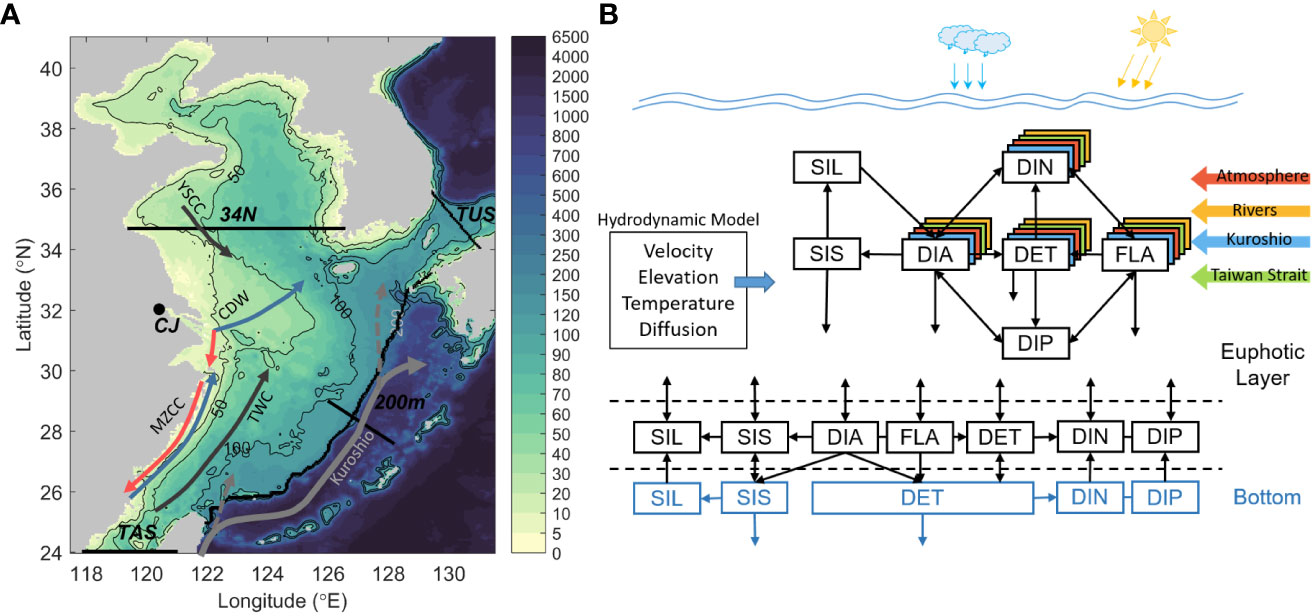
Figure 1 (A) Model domain and bathymetric map of the ECS. (B) Schematic illustration of the biological module. The black contour lines in (A) represent the isobaths. The black dot on the coast denotes the location of the inflow from the Changjiang River (CJ), which is the main source of the riverine DIN. The thin black lines show the positions of the Taiwan Strait (TAS), Tsushima Strait (TUS), 34.7° N section (34N), PN section, and designated 200-m isobath section. Black arrows denote the Kuroshio and its branches (dashed lines), the Taiwan Warm Current (TWC), and the Yellow Sea Coastal Current (YSCC). Blue and red arrows denote the summer and winter directions of the Min-Zhe Coastal Current (MZCC) and the Changjiang Diluted Water (CDW), respectively.

2.2 The tracking module

The second part is a tracking module following the methods of Ménesguen et al. (2006). Biological state variables from different external sources are separately calculated in this module rather than as a whole. Only DIN-related variables are tracked here. Because, in contrast to nearshore ECS, offshore ECS is the key region for export production and DIN is a limiting nutrient there. In addition, the input fluxes of the DIN from various sources in the ECS are comparable. Since the Kuroshio contributes a significantly greater amount to DIP than rivers and the atmosphere, DIP-related tracking may result in an expected Kuroshio-dominated result. The DIN from any external sources has the same physical and biogeochemical processes as the total DIN. The governing equations in the tracking module are the same as those in the first module. A complete subset of equations (Equations 1-4) is added to address the DIN-related tracking variables DIN, DIA, FLA, and DET for each source:

$\begin{array}{ll}\begin{array}{c}\frac{\mathbf{\partial }{\mathbf{\text{DIN}}}_{\mathbf{\text{i}}}}{\mathbf{\partial }\mathbf{\text{t}}}\mathbf{=}\mathit{d}\mathit{i}\mathit{f}\mathit{f}({\mathbf{\text{DIN}}}_{\mathbf{\text{i}}})\mathbf{-}\mathit{a}\mathit{d}\mathit{v}({\mathbf{\text{DIN}}}_{\mathbf{\text{i}}})\mathbf{+}\mathit{r}\mathit{e}\mathit{s}\mathit{p}(\mathbf{\text{FLA}})\mathbf{\times }\frac{{\mathbf{\text{FLA}}}_{\mathbf{\text{i}}}}{\mathbf{\text{FLA}}}\hfill \\ \mathbf{+}\mathit{r}\mathit{e}\mathit{s}\mathit{p}(\mathbf{\text{DIA}})\mathbf{\times }\frac{{\mathbf{\text{DIA}}}_{\mathbf{\text{i}}}}{\mathbf{\text{DIA}}}\mathbf{-}\mathit{p}\mathit{p}(\mathbf{\text{FLA}}\mathbf{+}\mathbf{\text{DIA}})\mathbf{\times }\frac{{\mathbf{\text{DIN}}}_{\mathbf{\text{i}}}}{\mathbf{\text{DIN}}}\mathbf{+}\mathit{r}\mathit{e}\mathit{m}\mathit{i}({\mathbf{\text{DET}}}_{\mathbf{\text{i }}})\hfill \end{array}& (1)\end{array}$

$\begin{array}{ll}\begin{array}{c}\frac{\mathbf{\partial }{\mathbf{\text{DIA}}}_{\mathbf{\text{i}}}}{\mathbf{\partial }\mathbf{\text{t}}}\mathbf{=}\mathit{d}\mathit{i}\mathit{f}\mathit{f}({\mathbf{\text{DIA}}}_{\mathbf{\text{i}}})\mathbf{-}\mathit{a}\mathit{d}\mathit{v}({\mathbf{\text{DIA}}}_{\mathbf{\text{i}}})\mathbf{+}\mathit{p}\mathit{p}(\mathbf{\text{DIA}})\mathbf{\times }\frac{{\mathbf{\text{DIN}}}_{\mathbf{\text{i}}}}{\mathbf{\text{DIN}}}\hfill \\ \mathbf{-}\mathit{r}\mathit{e}\mathit{s}\mathit{p}(\mathbf{\text{DIA}})\mathbf{\times }\frac{{\mathbf{\text{DIA}}}_{\mathbf{\text{i}}}}{\mathbf{\text{DIA}}}\mathbf{-}\mathit{m}\mathit{o}\mathit{r}\mathit{t}({\mathbf{\text{DIA}}}_{\mathbf{\text{i}}})\hfill \end{array}& (2)\end{array}$

$\begin{array}{ll}\begin{array}{c}\frac{\mathbf{\partial }{\mathbf{\text{FLA}}}_{\mathbf{\text{i}}}}{\mathbf{\partial }\mathbf{\text{t}}}\mathbf{=}\mathit{d}\mathit{i}\mathit{f}\mathit{f}({\mathbf{\text{FLA}}}_{\mathbf{\text{i}}})\mathbf{-}\mathit{a}\mathit{d}\mathit{v}({\mathbf{\text{FLA}}}_{\mathbf{\text{i}}})\mathbf{+}\mathit{p}\mathit{p}(\mathbf{\text{FLA}})\mathbf{\times }\frac{{\mathbf{\text{DIN}}}_{\mathbf{\text{i}}}}{\mathbf{\text{DIN}}}\hfill \\ \mathbf{-}\mathit{r}\mathit{e}\mathit{s}\mathit{p}(\mathbf{\text{FLA}})\mathbf{\times }\frac{{\mathbf{\text{FLA}}}_{\mathbf{\text{i}}}}{\mathbf{\text{FLA}}}\mathbf{-}\mathit{m}\mathit{o}\mathit{r}\mathit{t}({\mathbf{\text{FLA}}}_{\mathbf{\text{i}}})\hfill \end{array}& (3)\end{array}$

$\begin{array}{ll}\begin{array}{c}\frac{\mathbf{\partial }{\mathbf{\text{DET}}}_{\mathbf{\text{i}}}}{\mathbf{\partial }\mathbf{\text{t}}}\mathbf{=}\mathit{d}\mathit{i}\mathit{f}\mathit{f}({\mathbf{\text{DET}}}_{\mathbf{\text{i}}})\mathbf{-}\mathit{a}\mathit{d}\mathit{v}({\mathbf{\text{DET}}}_{\mathbf{\text{i}}})\mathbf{+}\mathit{m}\mathit{o}\mathit{r}\mathit{t}({\mathbf{\text{FLA}}}_{\mathbf{\text{i}}})\hfill \\ \mathbf{+}\mathit{m}\mathit{o}\mathit{r}\mathit{t}({\mathbf{\text{DIA}}}_{\mathbf{\text{i}}})\mathbf{-}\mathit{r}\mathit{e}\mathit{m}\mathit{i}({\mathbf{\text{DET}}}_{\mathbf{\text{i }}})\hfill \end{array}& (4)\end{array}$

where the subscript i represents the DIN from the ith source. The adv and diff represent the physical terms advection and diffusion. The resp, pp, remi, and mort indicate the biological terms respiration, primary production, remineralization, and mortality. The terms for biological processes are separated following the ratio of each source of DIN concentration to the total DIN concentration.

Four external DIN sources in the ECS are considered here, namely, the Kuroshio (K), the Taiwan Strait (T), atmospheric deposition (A), and rivers (R). The nitrogen cycle of each source is processed independently by independent equations. For example, the DIN_K denotes DIN from the Kuroshio. The phytoplankton assimilates DIN_K and produces CHL_K. Then CHL_K becomes DET_K after mortality. DET_K is further decomposed and regenerates DIN_K.

The DIN concentration, phytoplankton, and detritus of the four external sources are set to zero at the beginning of the model run. The input fluxes of DIN from ten main rivers were from published data (Zhang, 1996; Liu et al., 2009). The total riverine DIN flux into the ECS is 1.24 kmol s^-1. The DIN flux from the Changjiang River into the ECS is 0.89 kmol s^-1, which accounts for approximately 80% of the total and plays a dominant role among all the rivers. The climatology data of atmospheric wet and dry depositions was from observations (Zhang et al., 2011). The nutrient concentrations needed for the lateral boundary conditions are climatological mean of observation data for the Taiwan Strait (Huang et al., 2019) and from the Japan Meteorological Agency for the Kuroshio east of the Taiwan Island.

2.3 Model validation

The tracking module is run for over 5 years until it reaches equilibrium, and the outcomes in the final year are analyzed here. The physical-biological coupled model has been fully verified that it can reproduce the climatology features of physical and biological variables in the ECS (Zhao and Guo, 2011; Wang et al., 2019; Zhang et al., 2019; Shen et al., 2021).

We compared the modelled surface climatology temperature and salinity with Chen (2009). The model results are similar with those in Chen (2009). The circulation of the ECS from the model results can demonstrate the most well-known features in current field (Zhang et al., 2019). We also made comparison between the modeled and observed DIN and CHL concentration distributions at PN line and northern ECS (Wang et al., 2019; Zhang et al., 2019). Similar features were identified for DIN and CHL in both our model results and observations. The tracking module has been applied to evaluate the roles of multisource nutrients in primary production (Zhang et al., 2019) and the riverine nitrogen budgets in the ECS (Zhang et al., 2021). These factors are critical for the reliability of the tracking module.

Here, we compare the annual-mean density, velocity normal to the section, DIN and DIP concentrations, and DIN and DIP fluxes at the PN section in Figure 2 with the measurements described in (Guo et al., 2012, Figure 3) to validate the model’s capability. The location of the PN section is shown in Figure 1. The potential density increases from around 23 ${\sigma }_{\theta }$ at the surface layer to over 27 ${\sigma }_{\theta }$ at the bottom (Figure 2A). Both the range and isopycnal patterns match the measurement. The maximum velocity over 0.8 m s^-1 is located at the surface layer of the shelf break (Figure 2B) which is the same as the observation. The velocity core demonstrates the main axis of the Kuroshio, and the velocity decreases from the core to its flanks and depth. The DIN and DIP concentrations generally rise with depth (Figures 2C, D). While the concentrations in the upper 200 m are not as low as those from the measurements, the ranges of DIN (5~35 mmol m^-3) and DIP (0.5~2.5 mmol m^-3) concentrations are comparable to the observations. The product of the DIN or DIP concentration and the velocity normal to the section is used to determine the DIN and DIP fluxes (Figures 2E, F). In both model and observation results, the largest DIN and DIP fluxes are seen at a depth of around 400 m. The maximum DIN and DIP fluxes (>8.0 and >0.6 mmol m^-2s^-1) have magnitudes that are in agreement with the measurements (Figure 3 in Guo et al., 2012).

Figure 2

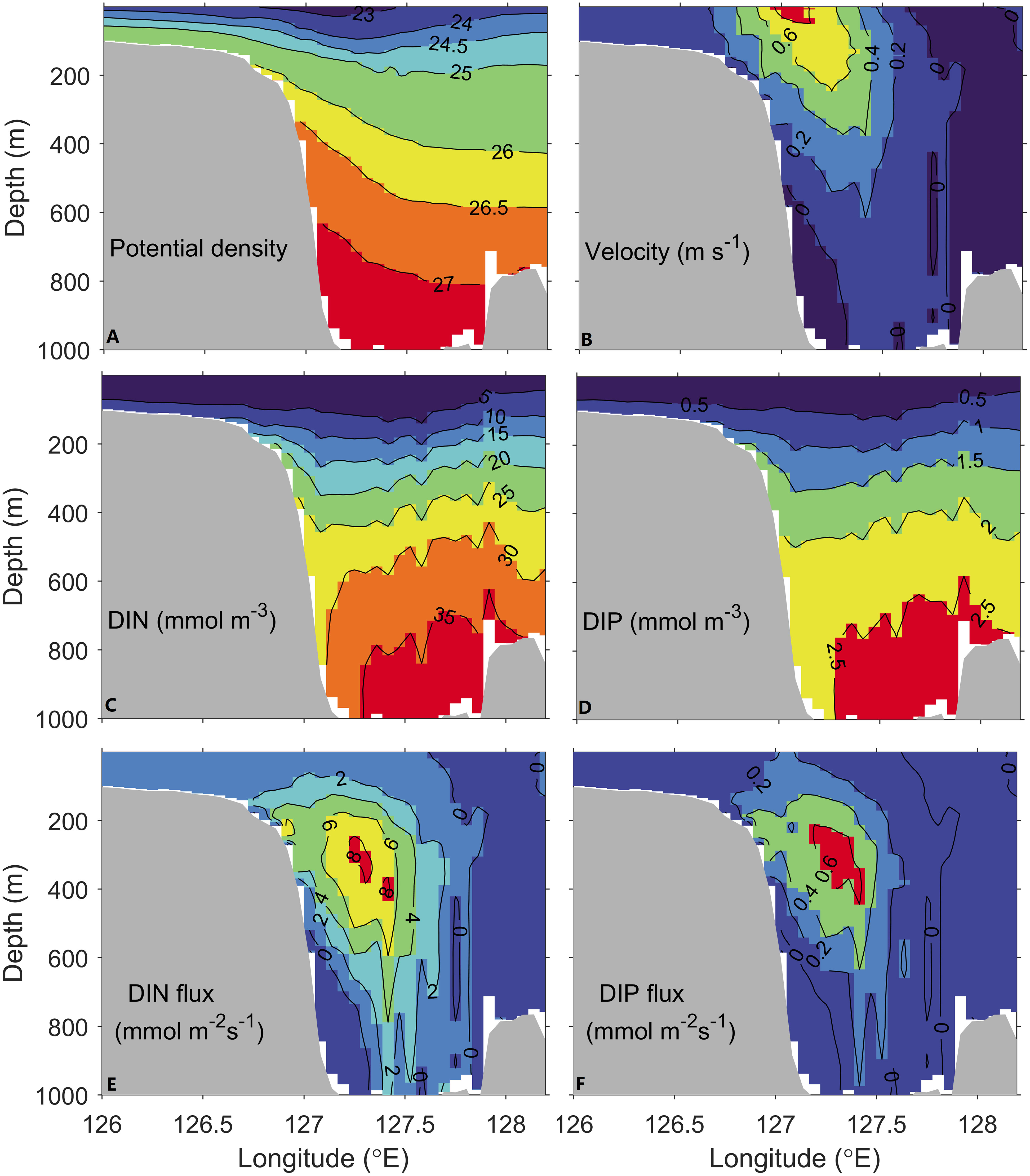
Figure 2 Annual-mean (A) potential density, (B) velocity normal to the section (m s^-1), (C) DIN and (D) DIP concentrations (mmol m^-3), (E) DIN and (F) DIP fluxes normal to the section (mmol m^-2s^-1) at the PN section from the model results.

Figure 3

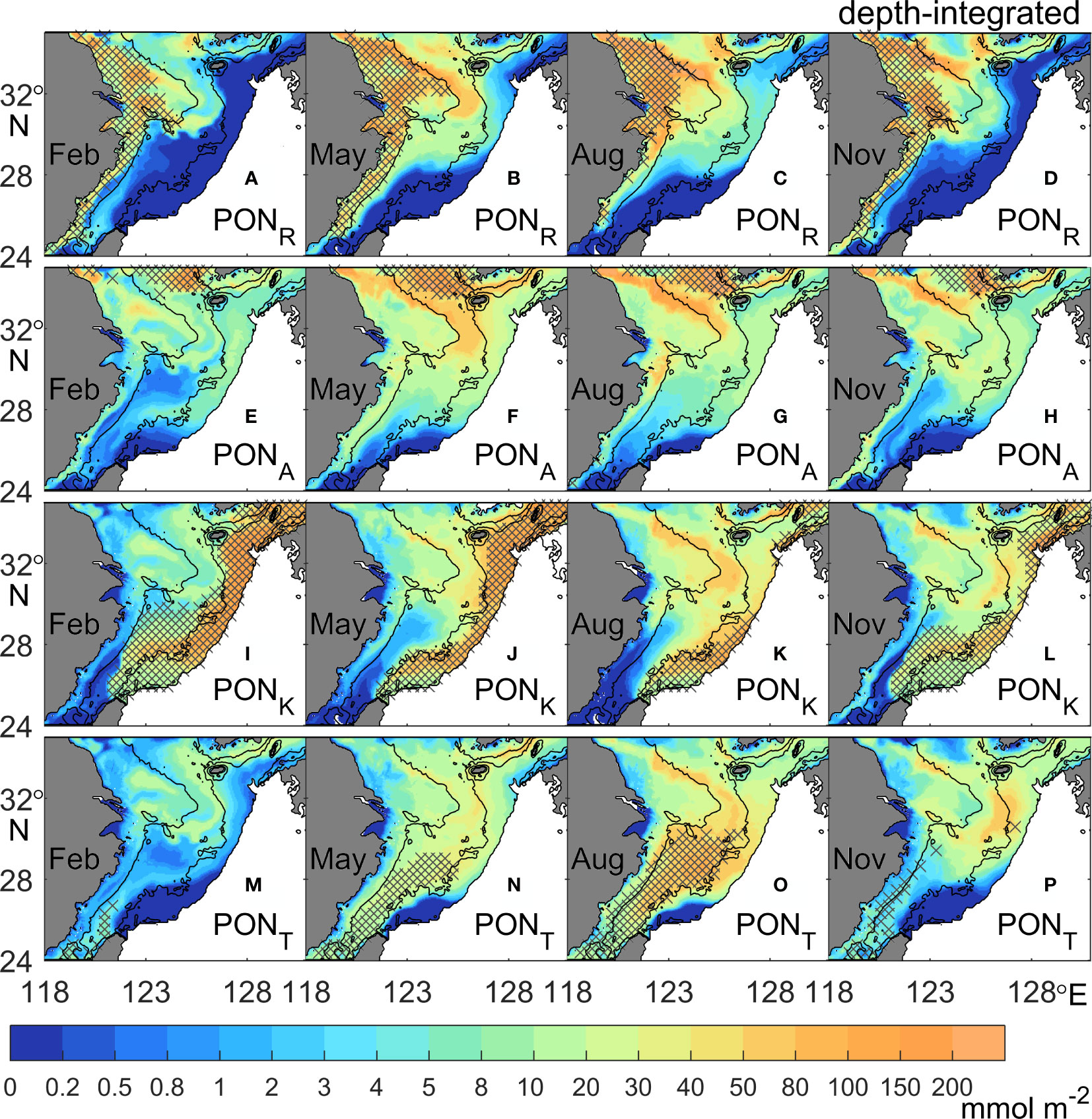
Figure 3 Seasonal distributions of depth-integrated PON concentrations (unit: mmol N m^-2) from different sources: (A–D) rivers (PON_R), (E–H) atmospheric deposition (PON_A), (I–L) the Kuroshio (PON_K), and (M–P) the Taiwan Strait (PON_T). The black contours denote the 50-m, 100-m, and 200-m isobaths. The concentration outside the shelf area is not shown. Cross hatching denotes that the PON concentration from a specific source comprises more than 50% of the total PON.

2.4 The calculation of DIN, CHL and DET inventories

The inventory is defined as the volume-integrated values for a variable concentration (Equation 5). Here we define the area shown in Figure 3 as our target region and calculate the monthly inventories of DIN, CHL, and DET, whose temporal variations are affected by biological and physical processes (Equation 6). Biological processes (denoted as Bio) are responsible for the transformation of DIN, CHL, and DET. The Bio term of DIN includes the remineralization of detritus, phytoplankton photosynthesis, and respiration (Equation 7). The Bio term for CHL involves respiration, mortality, and photosynthesis (Equation 8). The Bio term for DET includes its remineralization and phytoplankton mortality (Equation 9). The physical fluxes (denoted as Phy) include river input or atmospheric deposition (only for DIN), lateral transport across boundaries, and water–sediment flux at the sea bottom. A positive (negative) value of flux represents an increase (reduction) in the variable inventory. The time variation term (denoted by Tendency) refers to the sum of the physical and biological fluxes, which corresponds to the temporal change in inventory. The export production is based on the output flux of PON, which is referred to here as the sum of CHL and DET.

$\begin{array}{ll}inventor{\mathit{y}}_{\mathit{i}}\mathbf{=}\mathbf{\int }\mathbf{\int }\mathbf{\int }concentratio{\mathit{n}}_{\mathit{i}}\mathbf{·}dxdydz& (5)\end{array}$

$\begin{array}{ll}\begin{array}{c}\mathit{T}\mathit{e}\mathit{n}\mathit{d}\mathit{e}\mathit{n}\mathit{c}\mathit{y}\mathbf{ }\mathbf{=}\frac{\mathbf{\partial }inventor{\mathit{y}}_{\mathit{i}}}{\mathbf{\partial }\mathbf{\text{t}}}\mathbf{=}\mathit{P}\mathit{h}{\mathit{y}}_{\mathit{i}}\mathbf{+}\mathit{B}\mathit{i}{\mathit{o}}_{\mathit{i}}\hfill \\ \mathbf{=}\mathit{i}\mathit{n}\mathit{p}\mathit{u}\mathit{t}\mathbf{-}\mathit{o}\mathit{u}\mathit{t}\mathit{p}\mathit{u}\mathit{t}\mathbf{+}\mathit{b}\mathit{i}\mathit{o}\mathit{l}\mathit{o}\mathit{g}\mathit{i}\mathit{c}\mathit{a}\mathit{l}\mathit{s}\mathit{o}\mathit{u}\mathit{r}\mathit{c}\mathit{e}/\mathit{s}\mathit{i}\mathit{n}\mathit{k}\hfill \end{array}& (6)\end{array}$

$\begin{array}{ll}\begin{array}{c}Bio(DI{N}_{\mathit{i}})\mathbf{=}\mathbf{\int }\mathbf{\int }\mathbf{\int }(\mathit{r}\mathit{e}\mathit{s}\mathit{p}(F\mathbf{\text{LA}})\mathbf{\times }\frac{\mathbf{\text{FL}}{\mathbf{A}}_{\mathit{i}}}{\mathbf{\text{FLA}}}\mathbf{+}\mathit{r}\mathit{e}\mathit{s}\mathit{p}(\mathbf{\text{DIA}})\hfill \\ \mathbf{\times }\frac{{\mathbf{\text{DIA}}}_{\mathbf{\text{i}}}}{\mathbf{\text{DIA}}}\mathbf{-}\mathit{p}\mathit{p}(\mathbf{\text{FLA}}\mathbf{+}\mathbf{\text{DIA}})\mathbf{\times }\frac{{\mathbf{\text{DIN}}}_{\mathbf{\text{i}}}}{\mathbf{\text{DIN}}}\mathbf{+}\mathit{r}\mathit{e}\mathit{m}\mathit{i}({\mathbf{\text{DET}}}_{\mathbf{\text{i }}}))\mathbf{·}\mathbf{\text{dxdydz}}\hfill \end{array}& (7)\end{array}$

$\begin{array}{ll}\begin{array}{c}\mathbf{\text{Bio}}({\mathbf{\text{CHL}}}_{\mathit{i}})\mathbf{=}\mathbf{\int }\mathbf{\int }\mathbf{\int }(\mathit{p}\mathit{p}(\mathbf{\text{DIA}})\mathbf{\times }\frac{{\mathbf{\text{DIN}}}_{\mathbf{\text{i}}}}{\mathbf{\text{DIN}}}\mathbf{-}\mathit{r}\mathit{e}\mathit{s}\mathit{p}(\mathbf{\text{DIA}})\mathbf{\times }\frac{{\mathbf{\text{DIA}}}_{\mathbf{\text{i}}}}{\mathbf{\text{DIA}}}\hfill \\ \mathbf{-}\mathit{m}\mathit{o}\mathit{r}\mathit{t}({\mathbf{\text{DIA}}}_{\mathbf{\text{i}}})\mathbf{+}\mathit{p}\mathit{p}(\mathbf{\text{FLA}})\mathbf{\times }\frac{{\mathbf{\text{DIN}}}_{\mathbf{\text{i}}}}{\mathbf{\text{DIN}}}\mathbf{-}\mathit{r}\mathit{e}\mathit{s}\mathit{p}(\mathbf{\text{FLA}})\mathbf{\times }\frac{{\mathbf{\text{FLA}}}_{\mathbf{\text{i}}}}{\mathbf{\text{FLA}}}\hfill \\ \mathbf{-}\mathit{m}\mathit{o}\mathit{r}\mathit{t}({\mathbf{\text{FLA}}}_{\mathbf{\text{i}}}))\mathbf{·}\mathbf{\text{dxdydz}}\hfill \end{array}& (8)\end{array}$

$\begin{array}{ll}\begin{array}{c}\mathbf{\text{Bio}}({\mathbf{\text{DET}}}_{\mathit{i}})\mathbf{=}\mathbf{\int }\mathbf{\int }\mathbf{\int }(\mathit{m}\mathit{o}\mathit{r}\mathit{t}({\mathbf{\text{FLA}}}_{\mathbf{\text{i}}})\mathbf{+}\mathit{m}\mathit{o}\mathit{r}\mathit{t}({\mathbf{\text{DIA}}}_{\mathbf{\text{i}}})\hfill \\ \mathbf{-}\mathit{r}\mathit{e}\mathit{m}\mathit{i}({\mathbf{\text{DET}}}_{\mathbf{\text{i }}}))\mathbf{·}\mathbf{\text{dxdydz}}\hfill \end{array}& (9)\end{array}$

3 Results

3.1 Horizontal distributions of depth-integrated PON concentration

The detailed distributions of the depth-integrated PON concentrations from different sources are shown in Figure 3. The horizontal distributions of the depth-integrated DIN, CHL, and DET are shown in Supplementary Figures 1–3.

The PON_R is concentrated along the inner shelf (0~50 m) and plays a dominant role. The higher concentration of PON_R appears in the coastal areas north of the Changjiang Estuary in summer and autumn as the Changjiang Diluted Water (Figures 3C, D). The seasonal patterns of PON_R mainly follow those of DET_R (Supplementary Figure 3). The concentration of PON_A is higher on the northern middle shelf (50~100 m) and then decreases southward. It expands further in spring and summer (Figures 3F, G). Both PON_A and PON_R show the lowest concentrations in winter (Figures 3A, E).

The highest concentration of PON_K appears on the outer shelf (100~200 m) in winter (Figure 3I). In spring, the high-concentration area of PON_K narrows down to the southwest of Kyushu (Figure 3J). Unlike in winter and spring, the high-concentration area in summer appears northeast of Taiwan Island where the upwelling DIN_K can be converted to CHL_K and the DET_K effectively (Figure 3K and Supplementary Figures 2, 3). The obvious difference between the distributions of PON_K in winter and summer largely corresponds to seasonal variations in the Kuroshio intrusion, which flows onshore from the surface in winter and from the bottom in summer (Yang et al., 2012; Zhang et al., 2017). The pattern of PON_K in autumn is similar to that in summer but with a lower concentration (Figure 3L).

The concentration of PON_T is lowest among the four kinds of PON except in summer when the CHL_T and DET_T are largely produced (Supplementary Figures 2, 3) and has a maximum value on the southern middle shelf (Figure 3O). The high-concentration areas of PON_T mainly follow the Taiwan Warm Current and its branches (Liu et al., 2021).

3.2 Seasonal variations of inventories of DIN, CHL, and DET from each source

The seasonal variations of inventories of DIN, CHL, and DET are quite different between different sources (Figure 4). They are affected by biological and physical processes (bars in Figure 4, Equation 5). The inventory of DIN_R shows a peak value in March and a valley value in July (Figure 4A). The Bio term controls the variation of DIN_R and makes the inventory decrease in spring and summer. The enhancement of DIN_R from July to the next March is attributed to the reduced consumption by biological processes and gain from the river input in summer. The inventory of DIN_A shares similar seasonal patterns with DIN_R (Figure 4D). The correlation coefficient between DIN_A and DIN_R inventories is 0.97, which indicates a significant relationship. There was no significant correlation between the other DIN inventories.

Figure 4

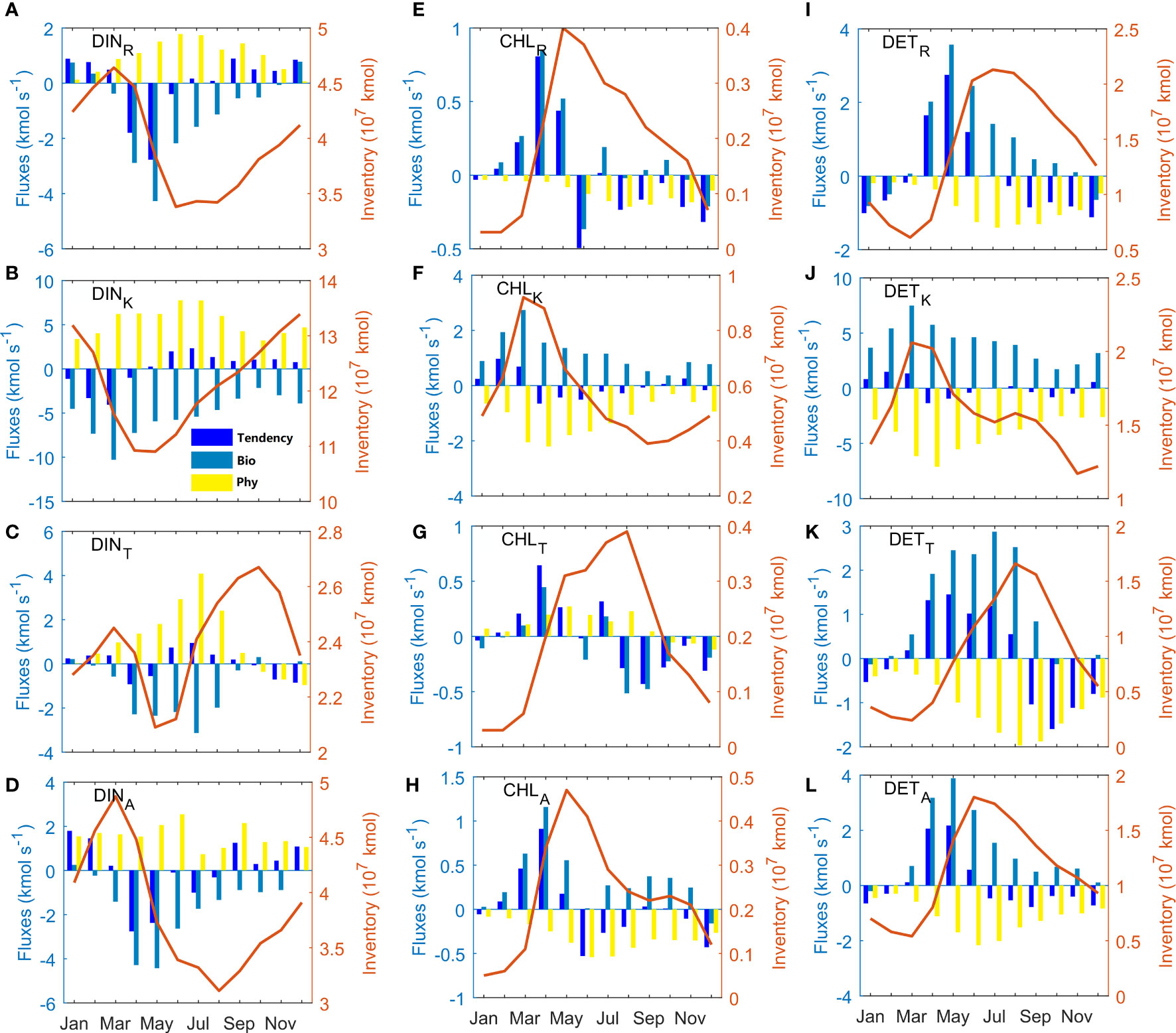
Figure 4 Monthly inventories (10⁷ kmol) of (A–D) DIN, (E–H) CHL, and (I–L) DET from sources of the rivers (R), the Kuroshio (K), the Taiwan Strait (T), and the atmospheric deposition (A) which are denoted by red lines. The blue, cyan, and yellow bars represent the time variation of inventory (Tendency), biological flux (Bio), and physical flux (Phy) with a unit of kmol s^-1. The biological and physical fluxes add up to the time variation of inventory. The positive (negative) value of flux induces an increase (decrease) in inventory.

The inventory of DIN_K plays a leading role in the quantity and seasonal amplitude (Figure 4B). It is highest in winter and lowest in April-May. The Bio term of DIN_K shows a negative value all year round, suggesting that the total biological processes spend the DIN_K. The seasonal variations of DIN_K follow its Bio term. The DIN_K inventory decreases from January to April due to the Bio term, then it increases sharply after May resulting from the physical flux.

The inventory of DIN_T is relatively low and changes weakly (Figure 4C). The DIN_T inventory reaches its maximum in October and its minimum in May-June. Unlike the Bio terms of the other sources with only one peak in spring, the Bio term of DIN_T has two peaks in April and July while the latter one is larger. The primary production supported by DIN_T mainly happens in the middle shelf resulting from the large volume transport and corresponding DIN_T input from the Taiwan Strait in summer (Zhang et al., 2019). The large DIN_T input in July makes its tendency term positive and increases the DIN_T inventory, even though the DIN_T consumption by biological processes also peaks.

The inventories of CHL_R and CHL_A change in phase with respect to DIN_A and DIN_R. Both of them peak in May and dissipate away in winter with a correlation coefficient of 0.95 (Figures 4E, H). The strong Bio terms of CHL_R and CHL_A dominate the time variations of their inventories. The CHL_K is still the largest among all the CHL at any time with a maximum in March and a minimum in autumn (Figure 4F). However, unlike CHL_R and CHL_A, the seasonal variations of the CHL_K inventory do not fully follow the Bio term, which is positive the whole year, even in winter. The strong Bio term of CHL_K gives a positive tendency term from January to March. But after April, the combined effects of enhanced Phy term and weakened Bio term make the tendency term of CHL_K below zero. The CHL_T inventory also shows low value in winter, and peaks in August (Figure 4G). It is significantly correlated to CHL_R and CHL_A with correlation coefficients of 0.91 and 0.77. The Bio term of CHL_T dominates the seasonal variations of tendency term, unlike the DIN_T situation.

The Bio term for DET comprises the mortality of phytoplankton and remineralization to DIN (Equation 9). The DET Bio term is positive most of the time, its peak time agrees with that of mortality of CHL (figure is not shown). The DET inventory from a specific source is markedly larger than the CHL inventory from the same source. The amplitudes of the four kinds of DET inventories are not much different. The superiority for Kuroshio source in DIN_K and CHL_K no longer exists in DET_K (Figure 4J). In March, the inventory of DET_K reaches its maximum, while the other three inventories of DET are the lowest. In the following June, July, and August, the maximum of DET_A, DET_R, and DET_T inventories appear one after another. The DET_R inventory is significantly large in summer and autumn due to the Bio term and then drops down with gradually increasing Phy term (Figure 4I). The Bio term of DET_R has the largest value in May, which is one month after the peak of CHL_R. In wintertime, the Bio term of DET_R is negative, indicating a stronger remineralization process than mortality. The Bio term of DET_T is largest in July when the CHL_T are produced in large numbers and a high temperature causes more mortality of phytoplankton (Figure 4K). The tendency term is therefore significantly above zero in spring and summer, which causes the DET_T inventory to increase and then drops to below zero in autumn. Comparing of these four kinds of DET, it is found that DET_R, DET_A and DET_T are correlated two by two, while DET_K is not correlated with any of the remaining three DET.

The annual means of each flux and inventory are shown in Supplementary Table 1. In the climatological model result, the inventories of the variables change little and the physical and biological fluxes are equivalent on a yearly basis. Over such a time scale, physical fluxes raise DIN inventories while biological activities reduce them. The CHL and DET, on the other hand, are produced by biological activities and exported by physical fluxes. Returning to seasonal variations, the peak times of Phy terms of CHL and DET lag those of Bio terms by one or a few months. That is because the outputs of the CHL and DET occur after a certain amount of accumulation of their inventory.

3.3 Seasonal variations of physical fluxes of DIN, CHL, and DET

The seasonal variations of each physical flux are shown in Figure 5. The physical fluxes include the DIN from rivers (Riv) and atmospheric deposition (Atm), the benthic fluxes (Bot), and the lateral transports across the Taiwan Strait (TAS), the 200-m isobath (200m), the Tsushima Strait (TUS) and the 34.7° N section (34N). The return of DIN from the sediment to the water column denotes the Bot flux of DIN, while that for CHL and DET is the net flux of resuspension and sinking.

Figure 5

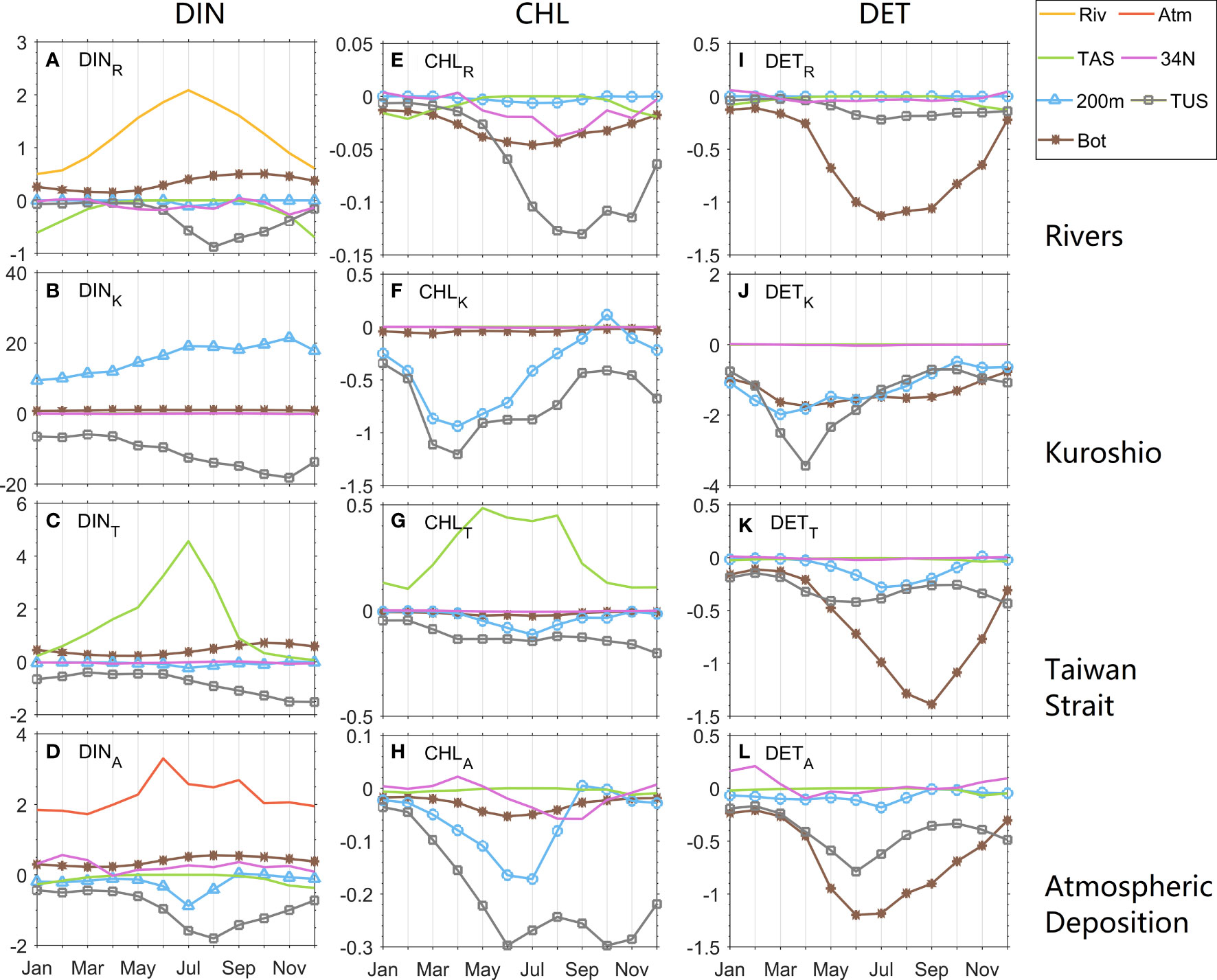
Figure 5 Monthly variations of physical fluxes of (A–D) DIN, (E–H) CHL, and (I–L) DET over the ECS shelf. The Riv and Atm terms refer to DIN input fluxes from rivers and the atmosphere. The fluxes across lateral sections are indicated by 200 m, TUS, TAS, and 34N (see Figure 1 for the position of each section). The flux across the water-sediment interface is denoted by Bot. Export production-related fluxes (200 m, TUS, and Bot) are shown by lines with markers. The positive (negative) value of flux induces an increase (decrease) in inventory.

The main physical flux of DIN_R is river input (Figure 5A). It is highest in summer like the river discharge. While benefiting from the large input from the river, the total inventory of DIN_R increases slowly after spring (Figure 4A). Meanwhile the high export of DIN_R to Tsushima Strait begins. The output flux of DIN_R through the Tsushima Strait is larger than other fluxes in the summer half year. The patterns of DIN_A fluxes are similar to those of DIN_R (Figure 5D) but it has a larger flux across 200-m isobath. The variation ranges of DIN_K fluxes are the largest among all the DIN sources (Figure 5B). The fluxes through the 200-m isobath and Tsushima Strait represent the main pathway of DIN_K, which intrudes across the 200-m isobath and exits via the Tsushima Strait. Therefore, their seasonal variations are almost in phase. Both reach a maximum in autumn when the Kuroshio onshore intrusion is highest (Guo et al., 2006; Zhao and Guo, 2011). The most prominent fluxes of DIN_T are input from the Taiwan Strait (Figure 5C).

From June to December, the CHL_R flux through the Tsushima Strait is distinct with a maximum in autumn (Figure 5E). The Bot flux of CHL_R is largest in summer with weak seasonal variation. The fluxes of CHL_K across the 200-m isobaths and the Tsushima Strait reach a maximum in April after the peak of the CHL_K inventory in March (Figures 4F, 5F). The flux through the Tsushima Strait is a little larger than that across 200-m isobaths throughout the year. The input of CHL_T from the Taiwan Strait is the dominant flux like the DIN_T situation (Figures 5C, G). It has two peaks in May and August. The maximum physical flux of CHL_A in summer results from the export through Tsushima Strait and 200-m isobath (Figure 5H).

The Bot terms show their important roles in all DET fluxes. The striking flux of DET_R is in the Bot terms (Figure 5I). The Bot term of the DET_R increases from April when the DET_R greatly increases. The largest two fluxes of DET_A are the Bot term and export to the Tsushima Strait (Figure 5L). Both the Bot term and export to the Tsushima Strait reach the maximum in June. The peak months of Bot fluxes of DET_R and DET_A are the same as those of their inventories. The Bot term of DET_T also plays a dominant role and it reaches the maximum one month after DET_T inventory peaks (Figure 5K). The seasonal variations in the DET_K fluxes are similar to those in the CHL_K fluxes except for a larger Bot flux (Figure 5J). The export fluxes of DET_K and CHL_K through three different exits (Bot, TUS, and 200m) show a comparable peak time in March or April.

3.4 Export production and e-ratio derived from different DIN sources over the ECS

In terms of long-term export production, the biogenic particles fluxes that are removed through the sediment and lateral boundaries to the open ocean are characterized as export production on the continental shelf. The main pathways of the export production over the ECS shelf are via the sediment and the Tsushima Strait to the Japan Sea and across the 200-m isobath to the northwest Pacific Ocean.

In the ECS, the particulate organic carbon to PON ratio approaches the Redfield ratio of 6.63, with a mean values ranging from 4 to 8 (Hung et al., 2000; Zhu et al., 2006). The PON fluxes may be utilized to estimate the organic carbon flux in this situation. The overall export production over the ECS is 6.83 kmol N s^-1 (=17.16 Tg C yr^-1) using a C/N ratio of 6.63, and ranging from 10.35-20.71 Tg C yr^-1 when considering a C/N ratio of 4~8. The export production is composed of net-Bot, TUS, and 200 m fluxes (Table 1). This value is slightly lower than the atmospheric CO₂ absorption of 23.3 ± 13.50 Tg C yr^-1 (Guo et al., 2015), suggesting that export to the open ocean and seafloor can reflect efficient carbon sequestration. The benthic flux of 1.40 kmol N s^-1 (44.15×10⁹ mol yr^-1) is less than the burial flux of organic nitrogen at 75×10⁹ mol N yr^-1 (Chen and Wang, 1999) because the benthic flux here considers only ocean-generated nitrogen and excludes the input of terrestrial organic nitrogen, because they only comprise small portions of the total Changjiang River nitrogen input flux (Zhang et al., 2003; Kwon et al., 2018). The 200 m flux of 1.95 kmol N s^-1 (=4.89 Tg C yr^-1) is between the reported POC output flux of 0.25~1.7 Tg C yr^-1 (Deng et al., 2006; Jiao et al., 2018; Yuan et al., 2018) and 12.61 Tg C yr^-1 (Chen and Wang, 1999). The net-Bot flux and the 200 m flux explain 20% and 29% of the total export production, respectively, while the TUS flux accounts for 51%. Consequently, approximately 80% of the total export production leaves by lateral transport. This value is consistent with the percentages of off-shelf transport and sediment burial of 80% and 20%, respectively, in eastern North America (Najjar et al., 2018), 70% and 30%, respectively, on the whole North American shelf (Fennel et al., 2019), and 60~100% and 40~0%, respectively, in northwest European continental shelf seas (Legge et al., 2020). However, this ratio varies among the PONs supported by four sources of nutrients, which is covered in the following subsection.

Table 1

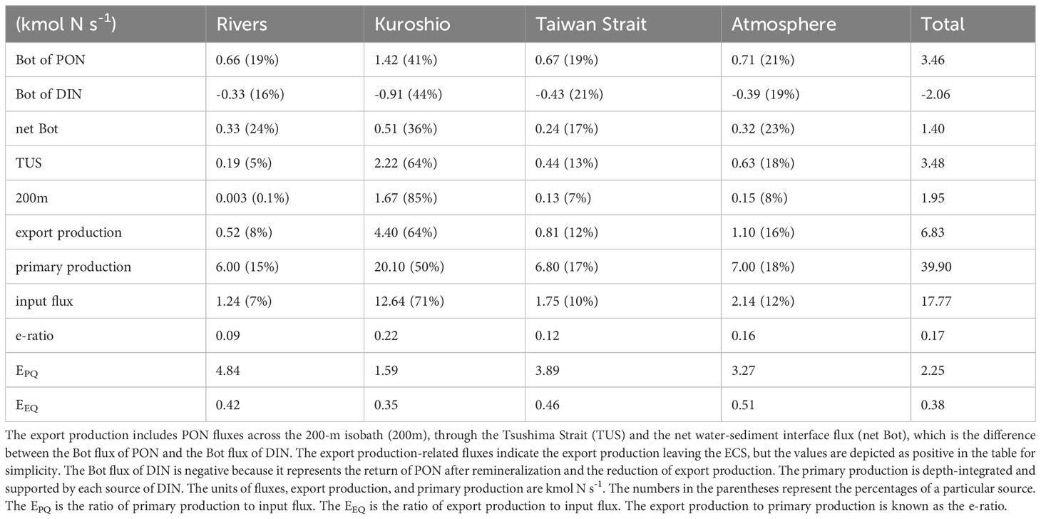
Table 1 Annual mean export production, primary production, and input fluxes from the four sources and their sum over the ECS.

The e-ratio is defined as the ratio of export production to primary production, which indicates the export efficiency of organic matter output from the generated carbon. The total primary production and export production are 39.9 and 6.83 kmol N s^-1, respectively, forming an e-ratio of 0.17. Our value is comparable to the result from the carbon budget based on a box model used by Chen and Wang (1999). They predicted an f-ratio of 0.15, which was supposed to balance the e-ratio in a steady state. Zuo et al. (2016) found that approximately 12% of the generated particulate nitrogen was exported between May and October in the ECS, which is less than our annual-averaged e-ratio due to the relatively high temperature and remineralization during their observation period. Based on corrected trap-collected POC fluxes, Hung et al. (2016) estimated an e-ratio of 0.59 nearshore and 0.16 offshore. The high e-ratio in the nearshore area demonstrated a significant vertical flux across the euphotic layer depth rather than efficient carbon export.

The export production values of PON from various sources have a wide range of features. The export production of PON_K is 4.40 kmol N s^-1, accounting for almost 64% of the total export production. The export production of PON_A is 1.10 kmol N s^-1, yet it accounts for 16%. The export production of PON_T accounts for 12%, while that of PON_R makes up only 8%. The PON_K net-Bot flux (0.51 kmol N s^-1) is the largest, accounting for nearly 36% of the overall net-Bot flux. The net-Bot fluxes of PON_R and PON_A are equivalent and account for approximately 23% of the total flux. The burial flux is larger in the coastal and shelf-break areas (Deng et al., 2006). Thus, the PON_T, which is mainly concentrated on the middle shelf, has a slightly lower net-Bot flux. The TUS flux of the PON_K has a fraction of 64%, whereas that of the PON_R has a fraction of 5%. The PON_K flux across the 200-m isobath accounts for 85% of the total, and the PON_R flux accounts for only 0.1%.

The primary export pathway for the PON_R is the sediment. The net-Bot flux of PON_R accounts for over 60% of the total export production of rivers. This ratio is disproportionate larger than the 20% for the total PON. The PON_R flux across the 200-m isobath is negligible. On a yearly basis, the impact of DIN_R and PON_R on the Kuroshio region is insignificant. The excess DIN_R and a small amount of PON_R may be exported through the Tsushima Strait (Isobe and Matsuno, 2008; Zhang et al., 2021). The PON_K flux is the largest through the Tsushima Strait, which benefits from the Kuroshio Branch Current west of Kyushu (Hsueh et al., 1996; Lie et al., 1998; Isobe, 2000) and the outflow through the Tsushima Strait to the Japan Sea (Isobe et al., 2002; Teague et al., 2003). The total lateral transport of PON_K (TUS and 200m) accounts for nearly 90% of the export production. The Tsushima Strait is also the principal export pathway for PON_T and PON_A, and the sediment is the second important export pathway. About 30% of the overall export production of PON_T and PON_A are made up of their net Bot fluxes, respectively. PON_T and PON_A are mostly found on the middle shelf (Figure 3), demonstrating a distinction between coastal PON_R and oceanic PON_K.

4 Discussion

We establish two other ratios to further compare the export efficiency of different sources. The E_PQ is defined as the ratio of primary production to the nitrogen input flux, and the E_EQ is the ratio of export production to the nitrogen input flux. The two ratios connect the input flux to the primary production responses and then to the final export production. The input flux of nitrogen is much smaller than that of primary production. The excess primary production is supported by recycled DIN rather than external input. Thus, the E_PQ denotes how many times the loaded DIN is assimilated for primary production (Takeoka, 1997). The annual mean nitrogen inventory over the ECS is almost unchanged in a climatological state, suggesting a balance between the input and output of nitrogen. Export production is an organic form of output. Most of the remaining material leaves the shelf in inorganic form. The E_EQ represents the ratio of organic export to input and is the product of the e-ratio and E_PQ.

Although the export production and primary production of different sources are fairly different, the e-ratio difference is not big. The primary production supported by DIN_K accounts for over half of the total. The remaining half is shared evenly among DIN_A, DIN_T, and DIN_R. The order of the primary production values supported by various DIN sources corresponds to the order of their export production values. The e-ratio of DIN_K is greatest at 0.22, followed by an e-ratio of DIN_A at 0.16. The DIN_T has a ratio of 0.12, whereas the DIN_R has a ratio of 0.09.

The unique oceanic sources of DIN_K and coastal sources of DIN_R provide the maximum and minimum e-ratios, respectively. The high e-ratio of DIN_K is due to its proximity to the outlets of the 200-m isobath and the Tsushima Strait, where the horizontal currents transport the PON_K off the shelf. The E_PQ and E_EQ values of DIN_K are both the lowest, most likely resulting from the notably large DIN_K input. The highest E_PQ of DIN_R (4.84) indicates that the input DIN_R is used by phytoplankton for nearly five times, and the generated PON_R is extensively recycled over the shelf and has difficulty reaching the lateral export pathways. This suggests that offshore rather than nearshore locations are usually great carbon sequestration sites.

A schematic representation of the different patterns of the nitrogen budgets from the Kuroshio and the rivers is shown in Figure 6. The cycle of DIN_K starts from the input from external sources the Kuroshio with a value of 12.64 kmol s^-1. A portion of DIN_K (5.31 kmol s^-1) is converted by biological processes into PON, while the remaining is exported through the Tsushima Strait (8.17 kmol s^-1). A value of 0.91 kmol s^-1 is provided to DIN_K by the benthic flux. The cycle of PON_K begins with the biological flux of 5.31 kmol s^-1. This value is equivalent to the sum of the fluxes through the sediment (1.42 kmol s^-1), the TUS (1.67 kmol s^-1), and 200m (2.22 kmol s^-1) fluxes. The fluxes of DIN_K and PON_K through other boundaries are negligible. The input of DIN_R (1.24 kmol s^-1) is only one-tenth of that from the Kuroshio and most of them (0.98 kmol s^-1) turn into PON_R. The primary exit of PON_R is the sediment rather than lateral boundaries.

Figure 6

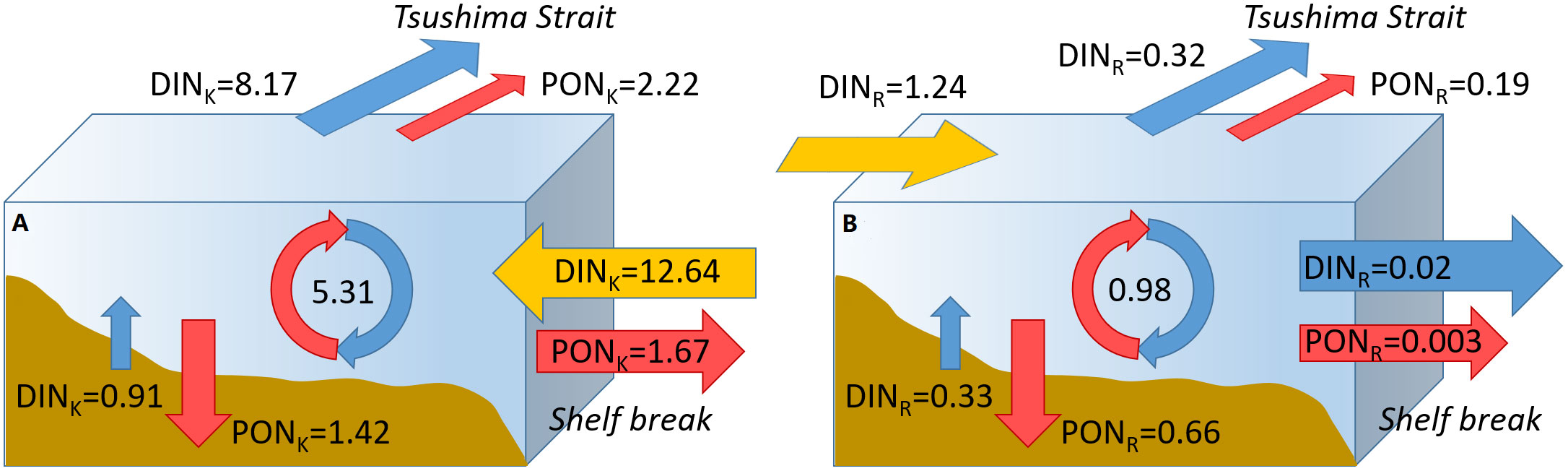
Figure 6 Annual-mean biological and export fluxes of (A) DIN_K and PON_K and (B) DIN_R and PON_R (unit: kmol s^-1). The yellow arrows represent the DIN input from the (A) Kuroshio and (B) rivers. The fluxes of DIN and PON through sediment, shelf break, and the Tsushima Strait are indicated by blue and red lines, respectively. The circles indicate the transformation from DIN to PON through biological activities.

The magnitudes of the E_PQ and e-ratio of DIN_A and DIN_T are between those of DIN_R and DIN_K. However, the E_EQ of DIN_A and DIN_T (0.51 and 0.46), which is the product of E_PQ and the e-ratio, is higher than that of DIN_R and DIN_K. These two DIN values have higher primary production efficiency (Zhang et al., 2019) and an e-ratio that is not too low, thus approximately 50% of the input DIN_A and DIN_T are exported in organic form. This suggests that the ECS shelf efficiently processes them. The increasing inputs of DIN from the Taiwan Strait and atmosphere may lead to more export production and carbon sequestration.

5 Conclusions

The export production values derived from various nitrogen sources over the ECS are assessed using a three-dimensional physical-biological coupled model and a tracking technique. We begin with the distributions of PON supported by different sources. PON_K and PON_R concentrate offshore and nearshore, respectively, and PON_A and PON_T are found on the middle shelf. The variations in DIN and PON inventories are the combined effects of physical and biological processes. Physical fluxes raise DIN inventories while biological activities reduce them. For PON, the situation is the exact reverse. The export fluxes of PON occur after a certain amount of accumulation of their inventory.

There are two ways in which the mechanism of export production in the shelf seas differs from that in the ocean. Initially, organic matter in the shelf seas should be exported through the sediment rather than through the bottom of the euphotic layer. Second, the shelf seas pump organic matter laterally into the ocean. We use the PON fluxes to the seafloor and open ocean (via the Tsushima Strait to the Japan Sea and the shelf break to the Northwestern Pacific Ocean) to calculate the export production over the ECS, and the result is 6.83 kmol N s^-1. This value is slightly lower than the atmospheric CO₂ absorption. The Tsushima Strait is the principal export route (51%) for PON, followed by the shelf break (29%) and sea bottom (20%), suggesting the important role of off-shelf transport.

The various roles of PON in export production and e-ratio are influenced by its distribution. The PON supported by the nutrients from the Kuroshio concentrates on the outer shelf and contributes to 64% of the overall export production, whereas the PON supported by the nutrients from rivers concentrates in the coastal area and accounts for only 8% of the overall export production, which demonstrates that offshore areas are vital locations for carbon sequestration.

Data availability statement

The raw data supporting the conclusions of this article will be made available by the authors, without undue reservation.

Author contributions

JZ: Writing – original draft. LeZ: Visualization, Writing – review & editing. XG: Conceptualization, Writing – review & editing. YW: Methodology, Writing – review & editing. JF: Writing – review & editing. LiZ: Conceptualization, Writing – review & editing.

Funding

The author(s) declare financial support was received for the research, authorship, and/or publication of this article. This word was supported by the National Natural Science Foundation of China [grant numbers 42006018, 41876018, 42176198]; Grants-in-Aid for Scientific Research [MEXT KAKENHI, grant numbers 22H05206]; the Tianjin Municipal Education Commission Scientific Research Project [grant number 2019KJ219]. JZ thanks the support of the Ministry of Education, Culture, Sports, Science and Technology, Japan (MEXT) under a Joint Usage/Research Center, Leading Academia in Marine and Environment Pollution Research (LaMer) Project.

Conflict of interest

The authors declare that the research was conducted in the absence of any commercial or financial relationships that could be construed as a potential conflict of interest.

Publisher’s note

All claims expressed in this article are solely those of the authors and do not necessarily represent those of their affiliated organizations, or those of the publisher, the editors and the reviewers. Any product that may be evaluated in this article, or claim that may be made by its manufacturer, is not guaranteed or endorsed by the publisher.

Supplementary material

The Supplementary Material for this article can be found online at: https://www.frontiersin.org/articles/10.3389/fmars.2024.1338835/full#supplementary-material

References

Chen C. (2003). Physical-biological sources for dense algal blooms near the Changjiang River. Geophys. Res. Lett. 30, 1–4. doi: 10.1029/2002GL016391

CrossRef Full Text | Google Scholar

Chen C. T. A. (2009). Chemical and physical fronts in the Bohai, Yellow and East China seas. J. Mar. Syst. 78, 394–410. doi: 10.1016/j.jmarsys.2008.11.016

CrossRef Full Text | Google Scholar

Chen C. T. A., Wang S. L. (1999). Carbon, alkalinity and nutrient budgets on the East China Sea continental shelf. J. Geophys. Res. Ocean. 104, 20675–20686. doi: 10.1029/1999jc900055

CrossRef Full Text | Google Scholar

Deng B., Zhang J., Wu Y. (2006). Recent sediment accumulation and carbon burial in the East China Sea. Global Biogeochem. Cycles 20, 1–12. doi: 10.1029/2005GB002559

CrossRef Full Text | Google Scholar

Doney S. C. (2010). The growing human footprint on coastal and open-Ocean biogeochemistry. Science 80-. ), 328. doi: 10.1126/science.1185198

CrossRef Full Text | Google Scholar

Eppley R. W., Peterson B. J. (1979). Particulate organic matter flux and planktonic new production in the deep ocean. Nature 282, 677. doi: 10.1038/282677a0

CrossRef Full Text | Google Scholar

Fennel K. (2010). The role of continental shelves in nitrogen and carbon cycling: Northwestern North Atlantic case study. Ocean Sci. 6, 539–548. doi: 10.5194/os-6-539-2010

CrossRef Full Text | Google Scholar

Fennel K., Alin S., Barbero L., Evans W., Bourgeois T., Cooley S., et al. (2019). Carbon cycling in the North American coastal ocean: A synthesis. Biogeosciences 16, 1281–1304. doi: 10.5194/bg-16-1281-2019

CrossRef Full Text | Google Scholar

Guo X., Hukuda H., Miyazawa Y., Yamagata T. (2003). A triply nested ocean model for simulating the kuroshio-roles of horizontal resolution on JEBAR. J. Phys. Oceanogr. 33, 146–169. doi: 10.1175/1520-0485(2003)033<0146:ATNOMF>2.0.CO;2

CrossRef Full Text | Google Scholar

Guo X., Miyazawa Y., Yamagata T. (2006). The kuroshio onshore intrusion along the shelf break of the East China Sea: The origin of the tsushima warm current. J. Phys. Oceanogr. 36, 2205–2231. doi: 10.1175/JPO2976.1

CrossRef Full Text | Google Scholar

Guo X. H., Zhai W. D., Dai M. H., Zhang C., Bai Y., Xu Y., et al. (2015). Air-sea CO2 fluxes in the East China Sea based on multiple-year underway observations. Biogeosciences 12, 5415–5514. doi: 10.5194/bg-12-5495-2015

CrossRef Full Text | Google Scholar

Guo X., Zhu X.-H. X. H., Wu Q. S. Q.-S., Huang D. (2012). The Kuroshio nutrient stream and its temporal variation in the East China Sea. J. Geophys. Res. Ocean. 117, C1026. doi: 10.1029/2011JC007292

CrossRef Full Text | Google Scholar

Hong Q., Peng S., Zhao D., Cai P. (2021). Cross-shelf export of particulate organic carbon in the northern South China Sea: Insights from a 234Th mass balance. Prog. Oceanogr. 193, 102532. doi: 10.1016/j.pocean.2021.102532

CrossRef Full Text | Google Scholar

Hsueh Y., Lie H. J., Ichikawa H. (1996). On the branching of the Kuroshio west of Kyushu. J. Geophys. Res. 101, 3851–3857. doi: 10.1029/95jc03754

CrossRef Full Text | Google Scholar

Huang T. H., Chen C. T. A., Lee J., Wu C. R., Wang Y. L., Bai Y., et al. (2019). East China Sea increasingly gains limiting nutrient P from South China Sea. Sci. Rep. 9, 5648. doi: 10.1038/s41598-019-42020-4

PubMed Abstract | CrossRef Full Text | Google Scholar

Hung C. C., Chen Y. F., Hsu S. C., Wang K., Chen J. F., Burdige D. J. (2016). Using rare earth elements to constrain particulate organic carbon flux in the East China Sea. Sci. Rep. 6, 33880. doi: 10.1038/srep33880

PubMed Abstract | CrossRef Full Text | Google Scholar

Hung J. J., Lin P. L., Liu K. K. (2000). Dissolved and particulate organic carbon in the southern East China Sea. Cont. Shelf Res. 20, 545–569. doi: 10.1016/S0278-4343(99)00085-0

CrossRef Full Text | Google Scholar

Isobe A. (2000). Two-layer model on the branching of the Kuroshio southwest of Kyushu, Japan. J. Phys. Oceanogr. 30, 2461–2476. doi: 10.1175/1520-0485(2000)030<2461:tlmotb>2.0.co;2

CrossRef Full Text | Google Scholar

Isobe A., Ando M., Watanabe T., Senjyu T., Sugihara S., Manda A. (2002). Freshwater and temperature transports through the Tsushima-Korea Straits. J. Geophys. Res. 107, 3065. doi: 10.1029/2000JC000702

CrossRef Full Text | Google Scholar

Isobe A., Matsuno T. (2008). Long-distance nutrient-transport process in the Changjiang river plume on the East China Sea shelf in summer. J. Geophys. Res. Ocean. 113, C04006. doi: 10.1029/2007JC004248

CrossRef Full Text | Google Scholar

Jiao N., Liang Y., Zhang Y., Liu J., Zhang Y., Zhang R., et al. (2018). Carbon pools and fluxes in the China Seas and adjacent oceans. Sci. China Earth Sci. 61, 1535–1563. doi: 10.1007/s11430-018-9190-x

CrossRef Full Text | Google Scholar

Kelly T. B., Goericke R., Kahru M., Song H., Stukel M. R. (2018). Spatial and interannual variability in export efficiency and the biological pump in an eastern boundary current upwelling system with substantial lateral advection. Deep. Res. Part I 140, 14–25. doi: 10.1016/j.dsr.2018.08.007

CrossRef Full Text | Google Scholar

Kwon H. K., Kim G., Hwang J., Lim W. A., Park J. W., Kim T. H. (2018). Significant and conservative long-range transport of dissolved organic nutrients in the Changjiang diluted water. Sci. Rep. 8, 1–7. doi: 10.1038/s41598-018-31105-1

PubMed Abstract | CrossRef Full Text | Google Scholar

Laruelle G. G., Cai W.-J., Hu X., Gruber N., Mackenzie F. T., Regnier P. (2018). Continental shelves as a variable but increasing global sink for atmospheric carbon dioxide. Nat. Commun. 9, 454. doi: 10.1038/s41467-017-02738-z

PubMed Abstract | CrossRef Full Text | Google Scholar

Legge O., Johnson M., Hicks N., Jickells T., Diesing M., Aldridge J., et al. (2020). Carbon on the Northwest European shelf: contemporary budget and future influences. Front. Mar. Sci. 7. doi: 10.3389/fmars.2020.00143

CrossRef Full Text | Google Scholar

Lie H. J., Cho C. H., Lee J. H., Niiler P., Hu J. H. (1998). Separation of the Kuroshio water and its penetration onto the continental shelf west of Kyushu. J. Geophys. Res. 103, 2963–2976. doi: 10.1029/97jc03288

CrossRef Full Text | Google Scholar

Liu G., Chai F. (2009). Seasonal and interannual variability of primary and export production in the South China Sea: A three-dimensional physical-biogeochemical model study. ICES J. Mar. Sci. 66, 420–431. doi: 10.1093/icesjms/fsn219

CrossRef Full Text | Google Scholar

Liu Z., Gan J., Hu J., Wu H., Cai Z., Deng Y. (2021). Progress on circulation dynamics in the East China Sea and southern Yellow Sea: Origination, pathways, and destinations of shelf currents. Prog. Oceanogr. 193, 102553. doi: 10.1016/j.pocean.2021.102553

CrossRef Full Text | Google Scholar

Liu S. M., Hong G. H., Zhang J., Ye X. W., Jiang X. L. (2009). Nutrient budgets for large Chinese estuaries. Biogeosciences 6, 2245–2263. doi: 10.5194/bg-6-2245-2009

CrossRef Full Text | Google Scholar

Ménesguen A., Cugier P., Leblond I. (2006). A new numerical technique for tracking chemical species in a multi-source, coastal ecosystem, applied to nitrogen causing Ulva blooms in the Bay of Brest(France). Limnol. Oceanogr. 51, 591–601. doi: 10.4319/lo.2006.51.1_part_2.0591

CrossRef Full Text | Google Scholar

Muller-Karger F. E., Varela R., Thunell R., Luerssen R., Hu C., Walsh J. J. (2005). The importance of continental margins in the global carbon cycle. Geophys. Res. Lett. 32, L01602. doi: 10.1029/2004GL021346

CrossRef Full Text | Google Scholar

Najjar R. G., Herrmann M., Alexander R., Boyer E. W., Burdige D. J., Butman D., et al. (2018). Carbon budget of tidal wetlands, estuaries, and shelf waters of Eastern North America. Global Biogeochem. Cycles 32, 389–416. doi: 10.1002/2017GB005790

CrossRef Full Text | Google Scholar

Noman M. A., Sun J., Gang Q., Guo C., Islam M. S., Li S., et al. (2019). Factors regulating the phytoplankton and tintinnid microzooplankton communities in the East China Sea. Cont. Shelf Res. 181, 14–24. doi: 10.1016/j.csr.2019.05.007

CrossRef Full Text | Google Scholar

Qiu Y., Laws E. A., Wang L., Wang D., Liu X., Huang B. (2018). The potential contributions of phytoplankton cells and zooplankton fecal pellets to POC export fluxes during a spring bloom in the East China Sea. Cont. Shelf Res. 167, 32–45. doi: 10.1016/j.csr.2018.08.001

CrossRef Full Text | Google Scholar

Shen J. W., Zhao L., Zhang H. H., Wei H., Guo X. (2021). Controlling factors of annual cycle of dimethylsulfide in the Yellow and East China seas. Mar. pollut. Bull. 169, 112517. doi: 10.1016/j.marpolbul.2021.112517

PubMed Abstract | CrossRef Full Text | Google Scholar

Simpson J. H., Sharples J. (2012). Introduction to the Physical and Biological Oceanography of Shelf Seas (Cambridge, United Kingdom: Cambridge University Press).

Google Scholar

Skogen M., Søiland H. (1998). A user’s guide to NORWECOM v2.0: The NORWegian ECOlogical Model system (Bergen, Norway: Institute of Marine Research). Available at: http://scholar.google.com/scholar?hl=en&btnG=Search&q=intitle:A+User+’+s+Guide+to+NORWECOM+v2+.+0+,+a+coupled+3+dimensional+Physical+Chemical+Biological+Ocean-model#2.

Google Scholar

Skogen M. D., Svendsen E., Berntsen J., Aksnes D., Ulvestad K. B. (1995). Modelling the primary production in the North Sea using a coupled three-dimensional physical-chemical-biological ocean model. Estuar. Coast. Shelf Sci. 41, 545–565. doi: 10.1016/0272-7714(95)90026-8

CrossRef Full Text | Google Scholar

Stukel M. R., Benitez-Nelson C. R., Decima M., Taylor A. G., Buchwald C., Landry M. R. (2015). The biological pump in the Costa Rica Dome: An open-ocean upwelling system with high new production and low export. J. Plankton Res. 38, 348–365. doi: 10.1093/plankt/fbv097

PubMed Abstract | CrossRef Full Text | Google Scholar

Takeoka H. (1997). “Comparison of the Seto Inland Sea with other enclosed seas around the world,” in Sustainable Development in the Seto Inland Sea, Japan—From the Viewpoint of Fisheries. Eds. Okaichi T., Yanagi T. (Tokyo, Japan: Terra Scientific Publishing Company), 223–247.

Google Scholar

Teague W. J., Jacobs G. A., Ko D. S., Tang T. Y., Chang K. I., Suk M. S. (2003). Connectivity of the Taiwan, Cheju, and Korea straits. Cont. Shelf Res. 23, 63–77. doi: 10.1016/S0278-4343(02)00150-4

CrossRef Full Text | Google Scholar

Tsunogai S., Watanabe S., Sato T. (1999). Is there a “continental shelf pump” for the absorption of atmospheric CO2? Tellus Ser. B Chem. Phys. Meteorol. 51, 701–712. doi: 10.3402/tellusb.v51i3.16468

CrossRef Full Text | Google Scholar

Wang Y., Guo X., Zhao L., Zhang J. (2019). Seasonal variations in nutrients and biogenic particles in the upper and lower layers of East China Sea Shelf and their export to adjacent seas. Prog. Oceanogr. 176, 102138. doi: 10.1016/j.pocean.2019.102138

CrossRef Full Text | Google Scholar

Yang D., Yin B., Liu Z., Bai T., Qi J., Chen H. (2012). Numerical study on the pattern and origins of Kuroshio branches in the bottom water of southern East China Sea in summer. J. Geophys. Res. Ocean. 117, 1–16. doi: 10.1029/2011JC007528

CrossRef Full Text | Google Scholar

Yuan D., Hao J., Li J., He L. (2018). Cross-shelf carbon transport under different greenhouse gas emission scenarios in the East China Sea during winter. Sci. China Earth Sci. 61, 659–667. doi: 10.1007/s11430-017-9164-9

CrossRef Full Text | Google Scholar

Zhang J. (1996). Nutrient elements in large Chinese estuaries. Cont. Shelf Res. 16, 1023–1045. doi: 10.1016/0278-4343(95)00055-0

CrossRef Full Text | Google Scholar

Zhang J., Guo X., Zhao L. (2019). Tracing external sources of nutrients in the East China Sea and evaluating their contributions to primary production. Prog. Oceanogr. 176, 102122. doi: 10.1016/j.pocean.2019.102122

CrossRef Full Text | Google Scholar

Zhang J., Guo X., Zhao L. (2021). Budget of riverine nitrogen over the East China Sea shelf. Environ. pollut. 289, 117915. doi: 10.1016/j.envpol.2021.117915

PubMed Abstract | CrossRef Full Text | Google Scholar

Zhang J., Guo X., Zhao L., Miyazawa Y., Sun Q., Zhang J., et al. (2017). Water Exchange across Isobaths over the Continental Shelf of the East China Sea. J. Phys. Oceanogr. 47, 1043–1060. doi: 10.1175/JPO-D-16-0231.1

CrossRef Full Text | Google Scholar

Zhang S., Ji H., Yan W., Duan S. (2003). Composition and flux of nutrients transport to the Changjiang Estuary. J. Geogr. Sci. 13, 3–12. doi: 10.1007/bf02873141

CrossRef Full Text | Google Scholar

Zhang J., Zhang G. S., Bi Y. F., Liu S. M. (2011). Nitrogen species in rainwater and aerosols of the Yellow and East China seas: Effects of the East Asian monsoon and anthropogenic emissions and relevance for the NW Pacific Ocean. Global Biogeochem. Cycles 25, GB3020. doi: 10.1029/2010GB003896

CrossRef Full Text | Google Scholar

Zhao L., Guo X. (2011). Influence of cross-shelf water transport on nutrients and phytoplankton in the East China Sea: A model study. Ocean Sci. 7, 27–43. doi: 10.5194/os-7-27-2011

CrossRef Full Text | Google Scholar

Zhu Z. Y., Zhang J., Wu Y., Lin J. (2006). Bulk particulate organic carbon in the East China Sea: Tidal influence and bottom transport. Prog. Oceanogr. 69, 37–60. doi: 10.1016/j.pocean.2006.02.014

CrossRef Full Text | Google Scholar

Zuo J., Song J., Yuan H., Li X., Li N., Duan L. (2016). Particulate nitrogen and phosphorus in the East China Sea and its adjacent Kuroshio waters and evaluation of budgets for the East China Sea Shelf. Cont. Shelf Res. 131, 1–11. doi: 10.1016/j.csr.2016.11.003

CrossRef Full Text | Google Scholar