Improved capabilities of global ocean reanalyses for analysing sea level variability near the Atlantic and Gulf of Mexico Coastal U.S.

Realistic representation of monthly sea level anomalies in coastal regions has been a challenge for global ocean reanalyses. This is especially the case in coastal regions where sea levels are influenced by western boundary currents such as near the U.S. Atlantic Coast and the Gulf of Mexico. For these regions, most ocean reanalyses compare poorly to observations. Problems in reanalyses include errors in data assimilation and horizontal resolutions that are too coarse to simulate energetic currents like the Gulf Stream and Loop Current System. However, model capabilities are advancing with improved data assimilation and higher resolution. Here, we show that some current-generation ocean reanalyses produce monthly sea level anomalies with improved skill when compared to satellite altimetry observations of sea surface heights. Using tide gauge observations for coastal verification, we find the highest skill associated with the GLORYS12 and HYCOM ocean reanalyses. Both systems assimilate altimetry observations and have eddy-resolving horizontal resolutions (1/12°). We found less skill in three other ocean reanalyses (ACCESS-S2, ORAS5, and ORAP6) with coarser, though still eddy-permitting, resolutions (1/4°). The operational reanalysis from ECMWF (ORAS5) and their pilot reanalysis (ORAP6) provide an interesting comparison because the latter assimilates altimetry globally and with more weight, as well as assimilating ocean observations over continental shelves. We find these attributes associated with improved skill near many tide gauges. We also assessed an older reanalysis (CFSR), which has the lowest skill likely due to its lower resolution (1/2°) and lack of altimetry assimilation. ACCESS-S2 likewise does not assimilate altimetry, although its skill is much better than CFSR and only somewhat lower than ORAS5. Since coastal flooding is influenced by sea level anomalies, the recent development of skilful ocean reanalyses on monthly timescales may be useful for better understanding the physical processes associated with flood risks.

1 Introduction

Monitoring and forecasting sea level conditions is increasingly needed to support climate change adaption, particularly as ongoing sea level rise is contributing to more coastal flooding (Sweet and Park, 2014; Vitousek et al., 2017; Sweet et al., 2018; Thompson et al., 2021; Dusek et al., 2022). The U.S. Southeast Coast, stretching from Cape Hatteras (North Carolina) to Key West (Florida), is especially susceptible to flooding events, which are increasing in occurrence and severity (Sweet and Park, 2014; Wdowinski et al., 2016; Sweet et al., 2018; Volkov et al., 2023). Coastal flooding is becoming worse during severe storms, and destructive impacts are also happening more often during fair weather days (Sweet et al., 2018). Currently, there is a lack of tools to accurately predict coastal flooding, especially with the months-to-years lead time needed for actionable mitigation, like resource preparation and road closure planning.

High-tide flooding, which is sometimes referred to as either sunny-day or nuisance flooding (Moftakhari et al., 2017), is occurring more frequently now along the U.S. Atlantic and Gulf of Mexico coastal regions compared to past decades due to rising sea levels (Sweet et al., 2022) and changes in ocean circulation (Volkov et al., 2023). Many of these areas, hereafter referred to as the East and Gulf Coasts, are experiencing faster sea-level rise than the global average (Sallenger et al., 2012; Valle-Levinson et al., 2017). Regional and local variations in relative sea-level rise can be attributed to the pattern of ocean thermal expansion (e.g., Widlansky et al., 2020) and the global fingerprint of melting land ice (Stammer et al., 2013), along with local land subsidence as is widespread in many coastal parts of Texas and Louisiana (e.g., Liu et al., 2020). The largest differences in relative sea-level rise along the East and Gulf Coasts result from vertical land motion (including glacial isostatic adjustment), with smaller differences from thermal expansion, and melt fingerprints contributing the least (Harvey et al., 2021). When the sea-level rise trend combines with above-normal monthly sea levels, together with recurring phenomena like high tides, storm surges, heavy rainfall, or river runoff, threats to coastal communities are compounded (Wahl et al., 2015). The threat of compounded ocean events is especially pronounced in low-lying, densely populated areas like Charleston (South Carolina), where high-tide flooding is already a common occurrence (Sweet et al., 2018).

With the increasing occurrence of high-tide flooding along the East and Gulf Coasts, there is a growing need for sea level information to support coastal management as well as strategic planning for adaptation to future hazards (Kleinosky et al., 2007; Stephens et al., 2018). Much of this needed information could come from climate models in the form of understanding the components of high-tide flooding (Li et al., 2022b), providing future outlooks of sea level anomalies (e.g., Dusek et al., 2022), and describing sea level rise under various greenhouse warming scenarios (e.g., Yin et al., 2009). The issue, however, is that many global climate models are unable to realistically simulate the coastal ocean conditions in the northwestern Atlantic Ocean and Gulf of Mexico (Piecuch et al., 2016; Long et al., 2021). Sea level trends and monthly-to-decadal variability in the models are especially biased compared to observations in these areas, as well as in other western boundary current regions of the world’s oceans (Long et al., 2021; Widlansky et al., 2023).

Unfortunately, in the current generation of climate models, there is no seasonal forecasting skill for monthly sea level anomalies along the East Coast, in contrast to the skilful forecast capability for much of the Pacific Ocean including the U.S. West Coast (Long et al., 2021). In the tropical Pacific Islands, seasonal forecasts from climate models are routinely used to augment water-level outlooks from tide predictions based on astronomical cycles. This is performed by adding a sea level anomaly outlook for the next six months to the long-term trend of the local observed sea level (Widlansky et al., 2017). Long et al. (2021) showed in an assessment of ten climate models that the lack of seasonal forecasting skills for the East Coast exists as early as the lead-0 month. Assessing retrospective forecasts during that first month, correlations are mostly below 0.5 when verified against observed sea level anomalies from tide gauges such as at Fort Pulaski in Georgia. By the lead-6 month, forecast correlations with tide gauges on the Southeast Coast are near zero. Poor skill in forecasting sea level anomalies during the lead-0 month is especially concerning because this is a forecast time immediately after the model initialization, which is when we would hope forecast skill to be the highest. Furthermore, some of the most sophisticated forecasting systems also include satellite altimetry-measured sea level anomalies in their ocean data assimilations (e.g., Balmaseda et al., 2013), although with varying success in improving seasonal prediction of sea level near the coast (Widlansky et al., 2023).

Perhaps the poor skill of forecasting monthly coastal sea level anomalies should not be a surprise, particularly near western boundary regions where many global models show large uncertainties in simulating strong ocean currents such as the Gulf Stream (Chi et al., 2018). Piecuch et al. (2016) showed that none of the four global ocean model reanalyses available at the time could realistically describe the sea level conditions measured by tide gauges south of Cape Hatteras. Each of the reanalyses had a correlation below 0.6 at the interannual timescale assessed. North of Cape Hatteras, some of the reanalyses showed slightly better performance describing tide gauge observations, although surprisingly only for the Simple Ocean Data Assimilation (SODA) reanalysis as well as a barotropic model that had correlations between 0.7–0.8 (see Figure 5 in Piecuch et al., 2016 for a summary of the assessment, which also included the GECCO2, ORAS4, and GODAS reanalyses).

Problems in that previous generation of reanalyses have been attributed to a multitude of issues pertaining to model dynamics, physics, and initial conditions, which collectively affect the simulation of ocean variability. These ocean reanalyses appeared problematic in the Gulf of Mexico and throughout the northwestern Atlantic, especially near the wide continental shelf regions, perhaps because of biases in simulating the Loop Current and Gulf Stream as well as interactions of the currents with complex bathymetry (Calafat et al., 2018; Li et al., 2022a). Since the success of seasonal forecasting systems, as measured by the accuracy of predicting future sea level anomalies, is associated with the quality of the ocean initial conditions (i.e., as represented by the reanalysis/analysis product or approximately during the lead-0 month forecast; Long et al., 2021), the performance of current-generation ocean reanalyses needs to be assessed for the East and Gulf Coasts.

Advancements in ocean modelling since the reanalysis assessment of Piecuch et al. (2016) and forecasting assessment of Long et al. (2021), particularly regarding finer spatial resolutions, are expected to improve the simulation near the coast. Resolutions of earlier ocean reanalyses were typically between 1° to 2° latitude-longitude. Here, we assess reanalyses that use ocean models with nominal resolutions of 1/2°, 1/4°, or 1/12°. The latter category of much higher resolution is used by two of the reanalyses that will be assessed (i.e., the GLORYS12 and HYCOM products). Such an enhancement in model resolution facilitates a more faithful representation of ocean circulations and small-scale ocean features having a significant influence on coastal sea level variability, especially in eddy-rich regions of the Gulf of Mexico and in the Atlantic Ocean adjacent to the Gulf Stream.

There have also been substantial improvements in ocean data assimilation since the assessments of Piecuch et al. (2016) and Long et al. (2021). Models including altimetry assimilation have shown higher skill when close to the time of initialization, compared to similar models with no sea level observations assimilated (Widlansky et al., 2023). Questions remain though about how much to weigh the altimetry observations in the assimilation, especially in relatively shallow areas near the coast. Recently, the European Centre for Medium-Range Weather Forecasts (ECMWF) re-tuned the weighting of observations in their ocean assimilation technique for a pilot ocean data assimilation system. This included improvements for shallow depths that were not well assimilated by their otherwise similar operational system for ocean reanalysis and forecasting (Zuo et al., 2021). We will assess both ECMWF ocean reanalyses in this study, along with four other reanalyses that either do or do not assimilate altimetry. These are GLORYS12 and HYCOM, as well as a product from NOAA and one from the Australian Bureau of Meteorology. All six reanalyses are described in the next section.

The rest of this paper is organized as follows: Section 2 describes the sea level observations, reanalysis products, and assessment methodologies. Results are presented in Section 3, which is subdivided into investigations of how well the reanalyses represent the observed long-term trend, monthly-to-decadal variability, and coastal coherence of the variability. We conclude the paper by summarizing the results before discussing the remaining questions and research opportunities. The outcome of this study documents the capabilities of the current-generation ocean reanalyses and provides a foundation of new information supporting improved capabilities for monitoring, understanding, and forecasting coastal sea levels.

2 Data and methods

We assess sea level conditions in observations and ocean model reanalyses for the Northwestern Atlantic Ocean and Gulf of Mexico (i.e., within a broad area bounded by 20–50°N, 60–100°W). Our focus is on the near-coastal conditions during 1994–2020, which is a region and period well observed by an extensive tide gauge network and, to some extent, also by satellite altimetry. The data sets and procedures for assessing characteristics of interest, which include the sea level trends, climatology, and monthly anomalies, are described below.

The sea level observations consist of measurements from tide gauges and satellite altimetry. For both observation types (i.e., hourly water levels from tide gauges and daily sea levels from altimetry), we calculated monthly averages of the data. For 39 tide gauge stations located on the East and Gulf Coasts (Figure 1), we obtained the manually reviewed and quality-controlled “verified” data from NOAA’s Centre for Operational Oceanographic Products and Services (CO-OPS) Tides and Currents Archive. All the tide gauges have at least 72% completeness of hourly data during the assessment period from which we calculated monthly means provided at least 15 days of data were available in each calendar month. In cases of missing monthly data, we retained a gap in the time series. For altimetry, we used the 1/4° gridded daily absolute dynamic topography provided by the Copernicus Marine and Environment Monitoring Service (CMEMS) in delayed and near-real-time modes (pre- and post-October 2019, respectively), which are level-4 products derived by combining along-track data from multiple satellite missions. We calculate the monthly sea level anomaly of the altimetry data by subtracting the mean dynamic topography. It is important to note that the altimetry-measured sea level anomaly is with respect to a fixed reference level, whereas each tide gauge measures water level with respect to the local land elevation, which can change over time. Unlike the tide gauge measurements, the inverse-barometer (IB) effect is not included in our monthly sea level anomaly calculation from altimetry because the CMEMS product includes a dynamic atmospheric correction (DAC) to minimize potential aliasing associated with the timescale of satellite measurements. Likewise, none of the reanalyses include the IB effect (see Long et al., 2021 for a discussion of the IB effect in the context of seasonal sea level forecasting).

Figure 1

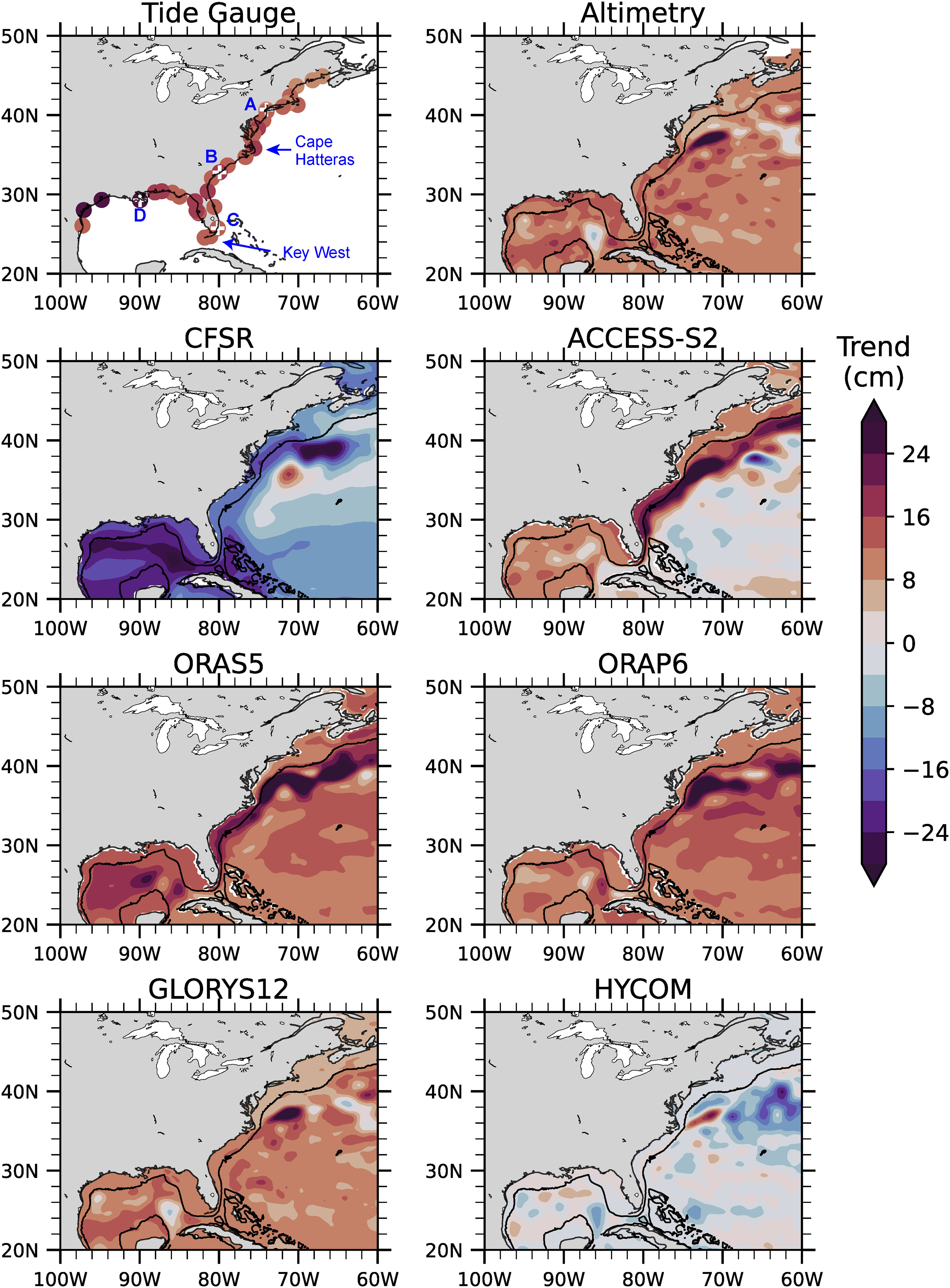
Figure 1 Linear trends of monthly sea level anomalies from the tide gauges, altimetry, and each of the reanalyses (cm; color bar). The 1994–2020 period is used throughout. In the tide gauge panel, filled dots with a plus marker (“+”) indicate the following locations: The Battery (A), Charleston (B), Virginia Key (C), and Grand Isle (D). Arrows point to Cape Hatteras and Key West. In the panels showing offshore results (throughout), the black contour indicates the 500 m isobath.

Monthly sea surface height (SSH) data acquired from six reanalysis products are compared with observations during the assessment period. Several of the datasets are combinations of reanalysis and analysis configurations (Table 1), with the latter being the real-time extension of the former, although we will refer to all the model data as reanalyses. Three reanalyses are based on modelling and assimilation systems that are also used for subseasonal-to-seasonal (S2S) forecasting: the National Centres for Environmental Prediction (NCEP) Climate Forecast System Reanalysis (CFSR; Saha et al., 2010, Saha et al., 2014), Australian Community Climate and Earth System Simulator-Seasonal version 2 (ACCESS-S2; Wedd et al., 2022) provided by the Bureau of Meteorology, and the Ocean ReAnalysis System 5 (ORAS5; Zuo et al., 2019) from ECMWF. We also include the Ocean ReAnalysis Pilot-6 (ORAP6; Zuo et al., 2021), which is a new product from ECMWF that uses a similar modelling configuration as ORAS5 (i.e., the same model and resolution) but has other major improvements, including updated atmospheric forcing, a new observation dataset, and improvements in the data assimilation method. Two noteworthy changes in the ORAP6 data assimilation system are that altimetry is given more weight globally in the assimilation and especially in coastal regions with water depth shallower than 500 m, which is where ocean observations were previously not assimilated. These changes in ORAP6 could significantly influence the simulation of coastal sea levels.

Table 1

Table 1 Description of the data products assessed in this study.

The remaining two reanalyses are not part of the S2S forecasting effort, but we include them because of their much higher-resolution ocean models: the HYCOM Global Ocean Forecasting System (GOFS 3.1; Metzger et al., 2014) and GLORYS12 global oceanic and sea ice reanalysis from CMEMS (Jean-Michel et al., 2021). Note that for HYCOM GOFS 3.1, data beyond February 2020 was excluded due to changes in the model grid, whereas all the other reanalyses are inclusive of the 1994–2020 period to overlap with the tide gauge and altimetry observations.

These six reanalyses have wide-ranging horizontal resolutions of their ocean models (Table 1). The ocean component of CFSR is the Modular Ocean Model (MOM) and it has the lowest horizontal resolution among the reanalyses (i.e., a 1/2° nominal resolution). ACCESS-S2, ORAS5, and ORAP6 use NEMO as their ocean model at a 1/4° eddy-permitting resolution. Both HYCOM GOF3.1 and GLORYS12 have a finer resolution at 1/12°, which should be sufficient to resolve most ocean eddy activity in our assessment region. GLORYS12 also uses the NEMO ocean model, whereas HYCOM GOFS 3.1 uses the HYCOM ocean model, which is how we will refer to that reanalysis.

The data assimilation systems are unique for each of the reanalyses. Altimetry assimilation is of particular importance for the consideration of sea level, especially in the subtropical and mid-latitude Atlantic where there is a relative scarcity of other observations such as subsurface temperature that could also capture the sea level variability (Widlansky et al., 2023). CFSR and ACCESS-S2 do not assimilate altimetry, whereas the other four reanalyses do (Table 1), although each assimilation system applies different weightings to the sea level observations. As mentioned above, ORAP6 includes altimetry assimilation in the shallower ocean compared to ORAS5, hence sea level observations closer to the coast have more weight in the newer reanalysis. We note that none of the reanalyses assimilate tide gauge observations, which is a potential opportunity for further improvement that we will discuss in Section 4.

We will be assessing measurements of coastal water levels (from tide gauges), sea levels (from altimetry), and SSH (from reanalyses). Throughout, we will refer to this data as describing the sea level. For all the monthly data during the 1994–2020 period, we calculated the linear trend, monthly climatology, and monthly anomalies. The latter calculation consists of subtracting the monthly climatology (i.e., annual cycle) and trend from the respective monthly data. For comparison with the Piecuch et al. (2016) assessment, we also calculated annual sea level anomalies by averaging monthly anomalies at coastal locations.

Performance, or skill, of the reanalyses as compared to observations will be measured using the following metrics. Differences of magnitude are used to compare the trends. Standard deviation (SD) indicates the amount of interannual variability. Anomaly correlation coefficient (ACC) indicates the association of variability between the observations and reanalyses. Root-mean-square error (RMSE) indicates the magnitude of errors, which are usually negatively associated with the ACC metric (i.e., typically greater errors when correlations with observations are weak). Note that errors in the sea levels from reanalyses are mostly normally distributed near the East and Gulf Coasts (i.e., skewness values are small; Supplementary Figures S1, S2 in Supplementary Material), thus the RMSE is a suitable metric for evaluating such errors (Hodson, 2022). These metrics are calculated location-wise for each grid point in the focus domain. In calculating the ACC and RMSE between altimetry and reanalyses, we used bilinear interpolation to re-grid the reanalyses to the altimetry grid. Otherwise, the altimetry and reanalyses are assessed on their native grids.

We also perform the skill assessment using time series to represent observations at or near tide gauges. Four locations will be considered as examples of the tide gauge observations: The Battery (New York), Charleston (South Carolina), Virginia Key (Florida), and Grand Isle (Louisiana). To compare the gridded data (altimetry and reanalyses) with in-situ data (tide gauges), we determine the three nearest-neighbour ocean grid points to each tide gauge and then calculate the average sea level using these points. We found this method to be rather insensitive to the chosen number of nearest grid points.

3 Results

Here, we report the results of assessing how well the reanalyses compare to the observed sea level. We will consider the long-term trend (Section 3.1), monthly-to-decadal variability (Section 3.2), and the coherence of variability along the coast (Section 3.3). We will describe the results regarding the open-ocean conditions as well as focusing on three parts of the U.S. Coast: Northeast, Southeast, and the Gulf. Cape Hatteras separates the former two coastlines, and Key West separates the latter (locations are labelled in Figure 1). We will thereby assess the ability of the reanalyses to depict the sea level conditions that affected the coastal U.S. from Maine to Texas.

3.1 Long-term trend

Figure 1 shows the long-term trends of sea level according to tide gauges, altimetry, and each of the reanalyses. The observations (i.e., tide gauges and altimetry) show that sea levels increased for the entire coast, and there is good agreement between the trends for most locations. The altimetry trend map also reveals increasing sea levels nearly everywhere assessed here (i.e., both near and away from the coast). One interesting difference between the tide gauge and altimetry trends is in the western Gulf of Mexico where the former has larger trends, which is explained by the different reference frames of these observations (see Section 2). Places where the tide gauge-measured trends are larger than the altimetry trends are likely to have experienced land subsidence (Kolker et al., 2011; Wöppelmann and Marcos, 2016; Ray et al., 2023), which is the case around many parts of the Texas and Louisiana Coasts. For example, during the 27-yr period, 26.2 cm of sea level rise was measured by the Grand Isle tide gauge but only 13.8 cm according to nearby altimetry observations, which are trends respectively equivalent to 9.70 mm/yr and 5.11 mm/yr. Supplementary Table S2 provides trend values for each of the 39 tide gauges, along with trends from the other datasets for these locations.

Overall, the spatial trends resemble that of the observations in only half of the reanalyses (ORAS5, ORAP6, and GLORYS12; Figure 1). Whereas all the reanalyses are produced using volume-conserving ocean models (i.e., preventing global mean sea level rise), the assimilation procedures of ORAS5, ORAP6, and GLORYS12 include adding a mass flux to match the altimetry-measured sea level rise (see Balmaseda et al., 2013 for the description of this process). The other three reanalyses (CFSR, ACCESS-S2, and HYCOM) do not include global sea level rise. CFSR has a negative trend of both global and regional sea levels due to unexplained drifts in the ocean density (Long et al., 2021). Even though global sea level rise is not included in ACCESS-S2, trends around the East Coast are much larger than observed (i.e., rising more than 24 cm near the Gulf Stream during the period). A similar trend bias is evident in ORAS5, and to some extent also in ORAP6, although the trend is clearly more realistic along the Southeast Coast in ORAP6. The trend pattern in HYCOM appears more reasonable compared to altimetry observations if the lack of global sea level rise is ignored. Of the six reanalyses, GLORYS12 shows the closest resemblance to the observed local sea level trends, particularly in comparison to altimetry (see again Supplementary Table S2 for results at specific locations).

3.2 Monthly-to-decadal variability

Sea level variability on monthly-to-decadal timescales contributes to the occurrence and severity of high-tide flooding (Dusek et al., 2022). The annual cycle dominates the sea level variability for the western boundary region of the Atlantic Ocean (Calafat et al., 2018), including in the Gulf of Mexico (Figure 2). Especially south of Cape Hatteras, the sea level annual cycles recorded by most tide gauges exceed 25 cm (i.e., the maximum minus minimum range of the monthly climatology). North of Cape Hatteras, the annual cycle ranges are smaller, and they are less than 10 cm north of Boston. The annual cycle range for altimetry near the coast shows a similar pattern as the tide gauges, although the ranges are somewhat smaller for altimetry, especially in the Gulf of Mexico as well as for the South Atlantic Bight, which extends from Cape Hatteras to the Upper Florida Keys.

Figure 2

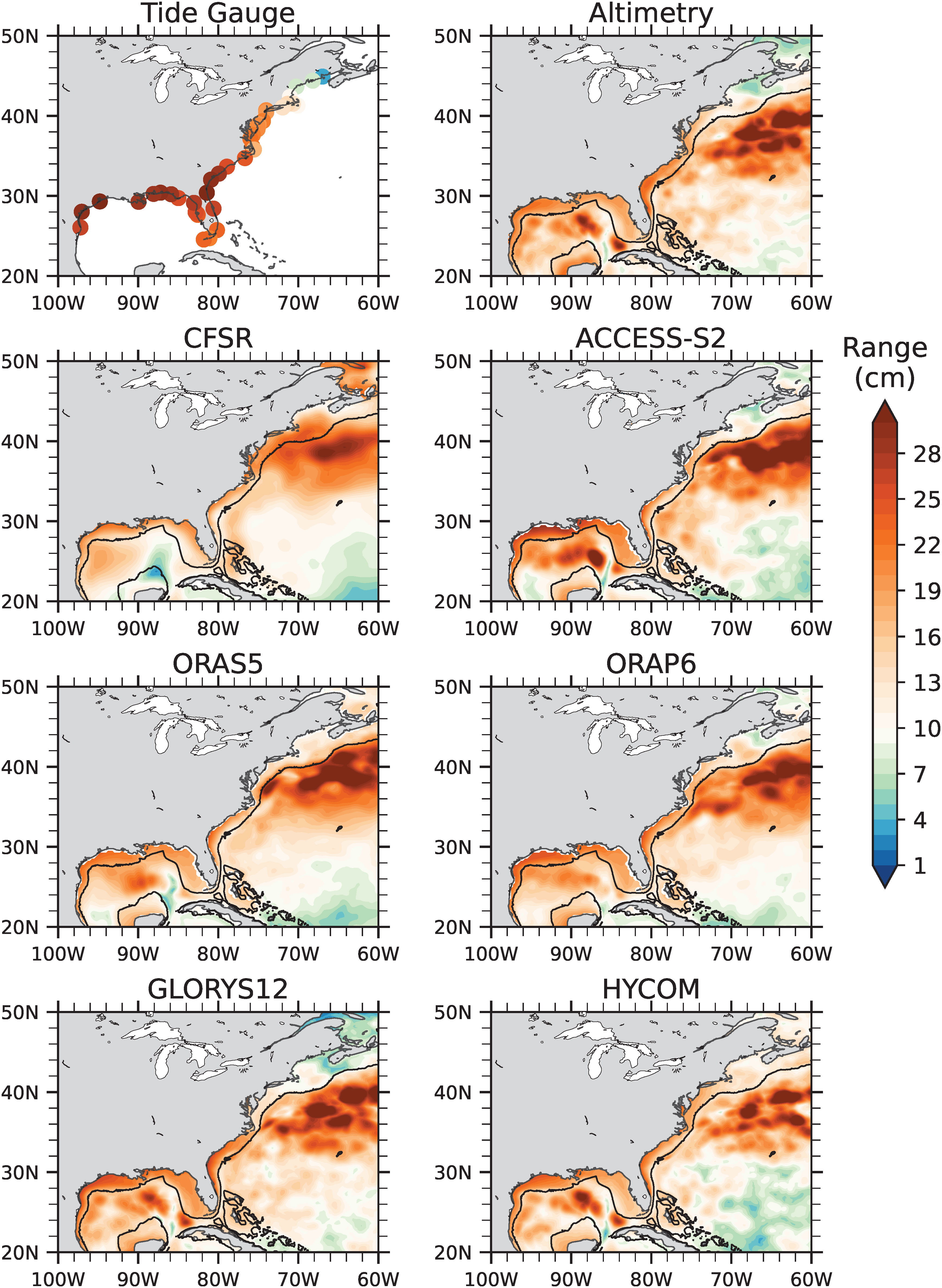
Figure 2 Range of sea level annual cycle from the tide gauges, altimetry, and each reanalysis (cm; color bar).

Comparison of the annual cycles in the reanalyses with either the tide gauges or altimetry observations reveals only subtle biases (Figure 2). All the reanalyses capture the observed sea level annual cycle pattern of ranges as well as timing (or seasonal phasing), both near the coast and offshore. Supplementary Figure S3 shows consistency in the peak months for sea levels across datasets, which typically occur either in September or October when the upper-ocean temperature is usually warmest for the East and Gulf Coasts. The sea level annual cycle in these places is mostly explained by thermal expansion (e.g., Widlansky et al., 2020). One notable bias is in CFSR, near the coast to the north of the typical Gulf Stream Extension region, where the annual cycle appears too large compared to the tide gauges and altimetry (Figure 2). Annual cycle biases in the other reanalyses are more subtle (Figure 2; see ACCESS-S2, ORAS5, ORAP6, GLORYS12, and HYCOM). This gives confidence that the sea level climatology is generally well resolved by the models and their assimilation of observations (primarily of the open ocean temperatures and, in the latter four assimilation systems, also sea levels from altimetry).

Figure 3 shows the amount of variability of the monthly sea level anomalies according to the SD metric described in Section 2. Everywhere along the coast, the SD magnitudes are below 10 cm, whereas there are offshore areas with more than three times as much variability (e.g., in the Loop Current System of the Gulf of Mexico as well as in the Gulf Stream Extension region). The largest coastal sea level variability recorded by tide gauges is in the Southeast and western Gulf regions (e.g., at Fort Pulaski and Galveston, respectively; see Supplementary Table S2). Similar patterns of variability are also observed in the altimetry observations. For most of the reanalyses, the sea level variability resembles observations, although the CFSR comparison is much weaker than for the others (e.g., too little variability south of Cape Hatteras and too much to the north). Overall, the variability pattern in higher-resolution reanalyses, especially GLORYS12 and HYCOM, appears more like the tide gauge and altimetry observations.

Figure 3

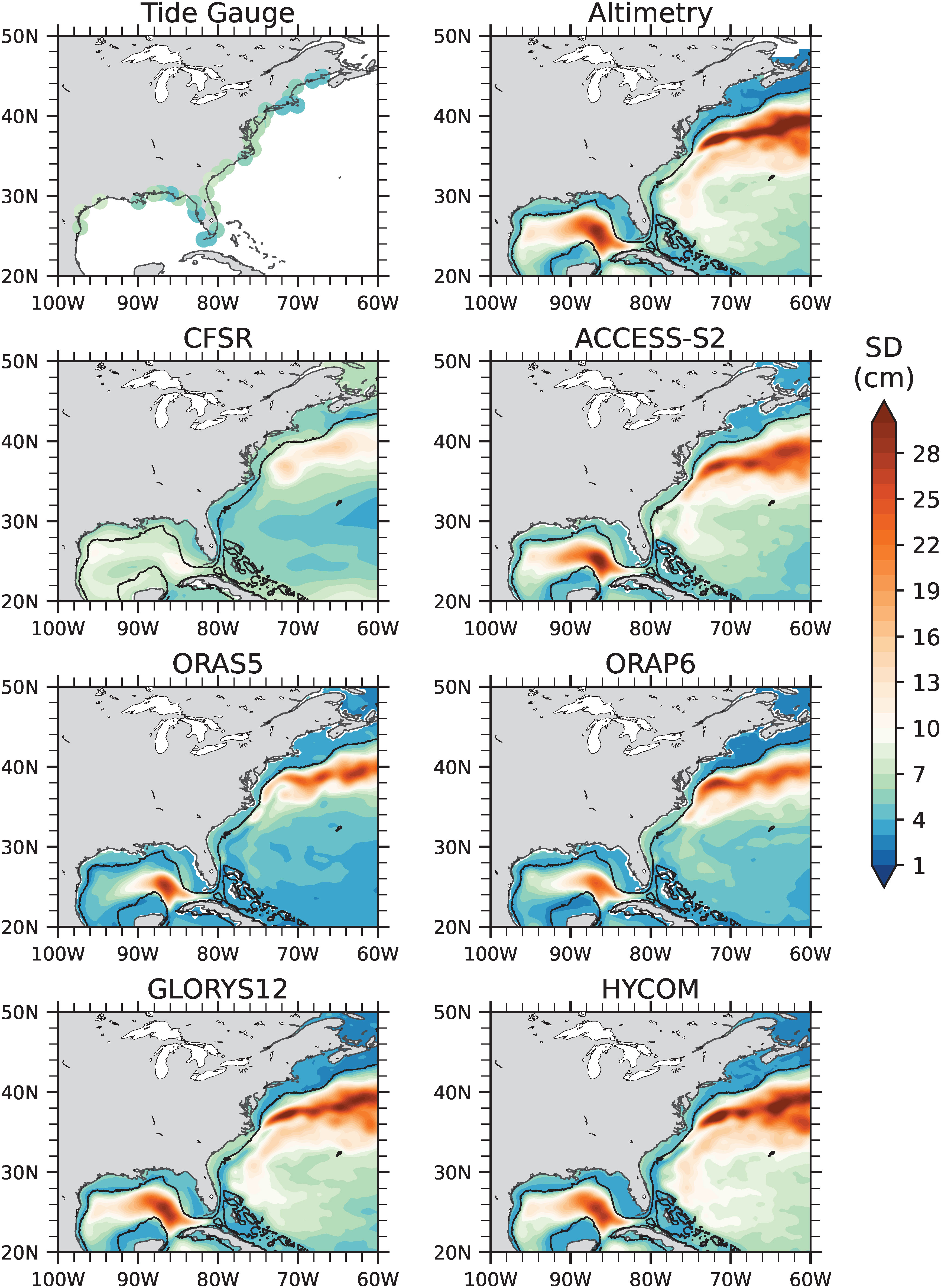
Figure 3 SD of monthly sea level anomalies from the tide gauges, altimetry, and each reanalysis (cm; color bar).

The quality of reanalyses in describing monthly sea level anomalies is revealed by comparing their correlations with observations and related errors (i.e., quantifying performances using ACC and RMSE metrics). We first use altimetry for the verification because this facilitates a comparison over the entire region (offshore and nearshore). Figures 4, 5 show the local ACC and RMSE, respectively, of each reanalysis compared with altimetry. Stark differences in the performance of the reanalyses are evident. Nearly everywhere, GLORYS12 and HYCOM clearly exhibit the highest ACC and the lowest RMSE. CFSR is the worst performing reanalysis, especially with regards to the ACC metric (Figure 4), although its RMSE is not noticeably different from ACCESS-S2, ORAS5, or ORAP6 in most places (coastal areas north of Cape Hatteras are an exception where all the reanalyses clearly perform better than CFSR; Figure 5).

Figure 4

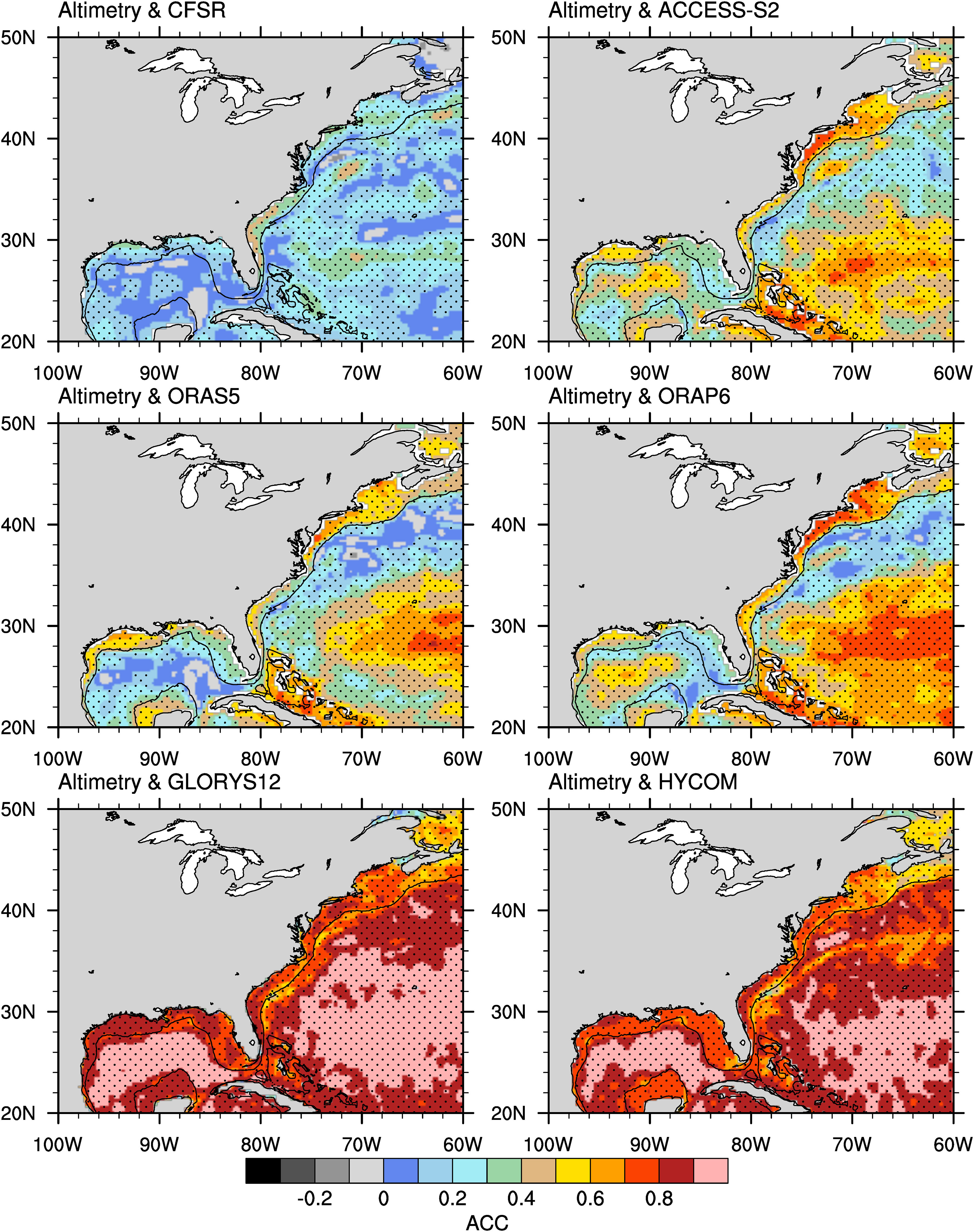
Figure 4 ACC of each reanalysis with altimetry monthly anomalies (color bar). Linear trends were removed from the data. Stippling indicates where the ACC is statistically significant at the 95% confidence level for 27 effective degrees of freedom.

Figure 5

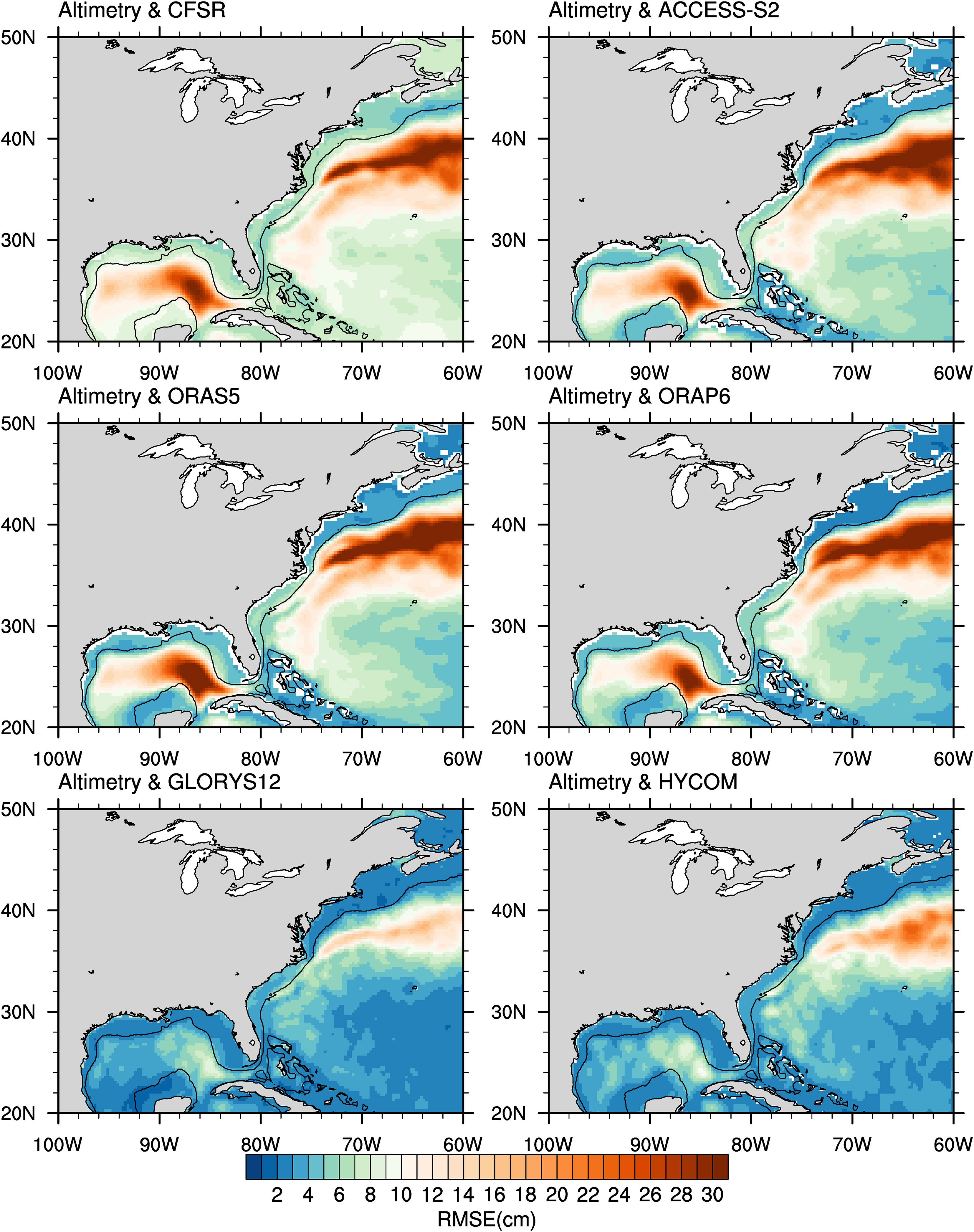
Figure 5 RMSE of each reanalysis relative to altimetry monthly anomalies (cm; color bar). Linear trends were removed from the data.

CFSR performs particularly poorly compared to the other reanalyses in most shallow regions near the coast, as outlined by the 500 m isobath in Figures 4, 5. One exception is for the South Atlantic Bight, where there is little difference between CFSR and ORAS5, despite the latter reanalysis having higher resolution and more advanced assimilation of observations, including altimetry away from the coast. ORAP6 applies more weight to altimetry in the ocean assimilation, including in areas shallower than 500 m, which is not the case for ORAS5. Comparisons of the ACC and RMSE metrics among these reanalyses (Figures 4, 5) suggest that ORAP6 is improved in most shallow areas near the East Coast, although differences for the Gulf Coast are more ambiguous. In any case, GLORYS12 and HYCOM compare most closely to altimetry, which is presumably because of their greater weighting of altimetry in ocean data assimilation and much higher resolutions compared to the other reanalyses.

Coastal sea levels are directly measured by tide gauges, and therefore are important observations for verifying the reanalyses. Figures 6, 7 present the ACC and RMSE relative to the tide gauges. The comparison reveals a strong association between altimetry and tide gauge observations, with an ACC of 0.88 for Charleston and similarly high values for most locations along the Southeast and Gulf Coasts. However, the ACC values are relatively lower north of Cape Hatteras (e.g., an ACC of 0.67 at The Battery and similar values for most of the Northeast Coast). The reason for this discrepancy between altimetry and tide gauges in the Northeast compared to the Southeast and Gulf Coasts is unclear. The IB effect explains a significant portion of the interannual sea level variability for the Northeast Coast (Piecuch and Ponte, 2015), which we also see by comparing the tide gauges with the DAC that was removed from the altimetry observations (Figures 6, 7). However, most of the reanalyses compare closer to the tide gauges along the Northeast Coast than the comparison with altimetry observations, even though neither the reanalyses nor the altimetry product includes the IB effect.

Figure 6

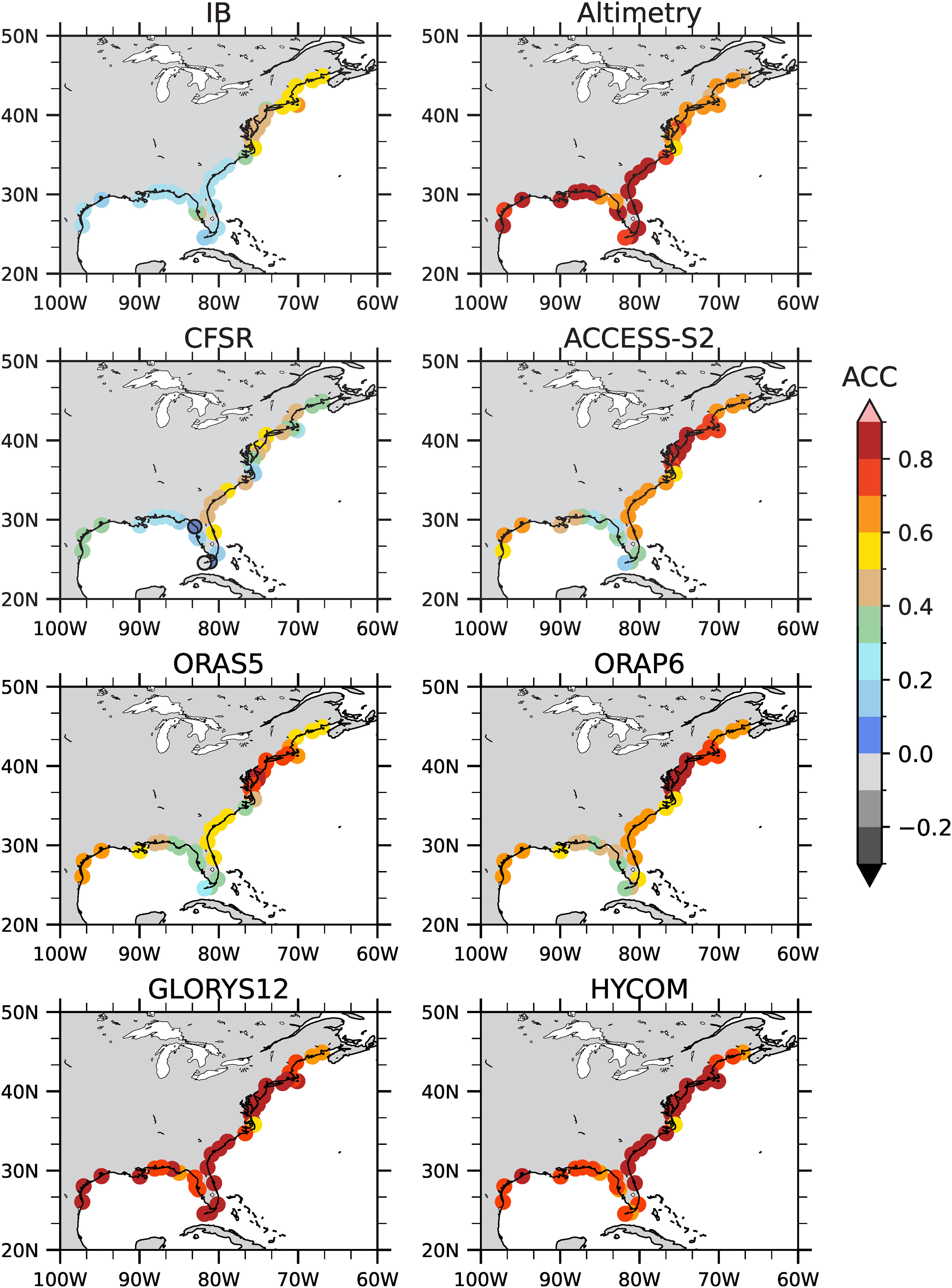
Figure 6 ACC of tide gauge monthly observations with the IB effect, altimetry, and each of the reanalyses (color bar). The IB effect is represented by the DAC that was applied to the altimetry measurements in making that product. All the ACC values are statistically significant at the 95% confidence level, except for the locations with outlined circles. Linear trends were removed from the data.

Figure 7

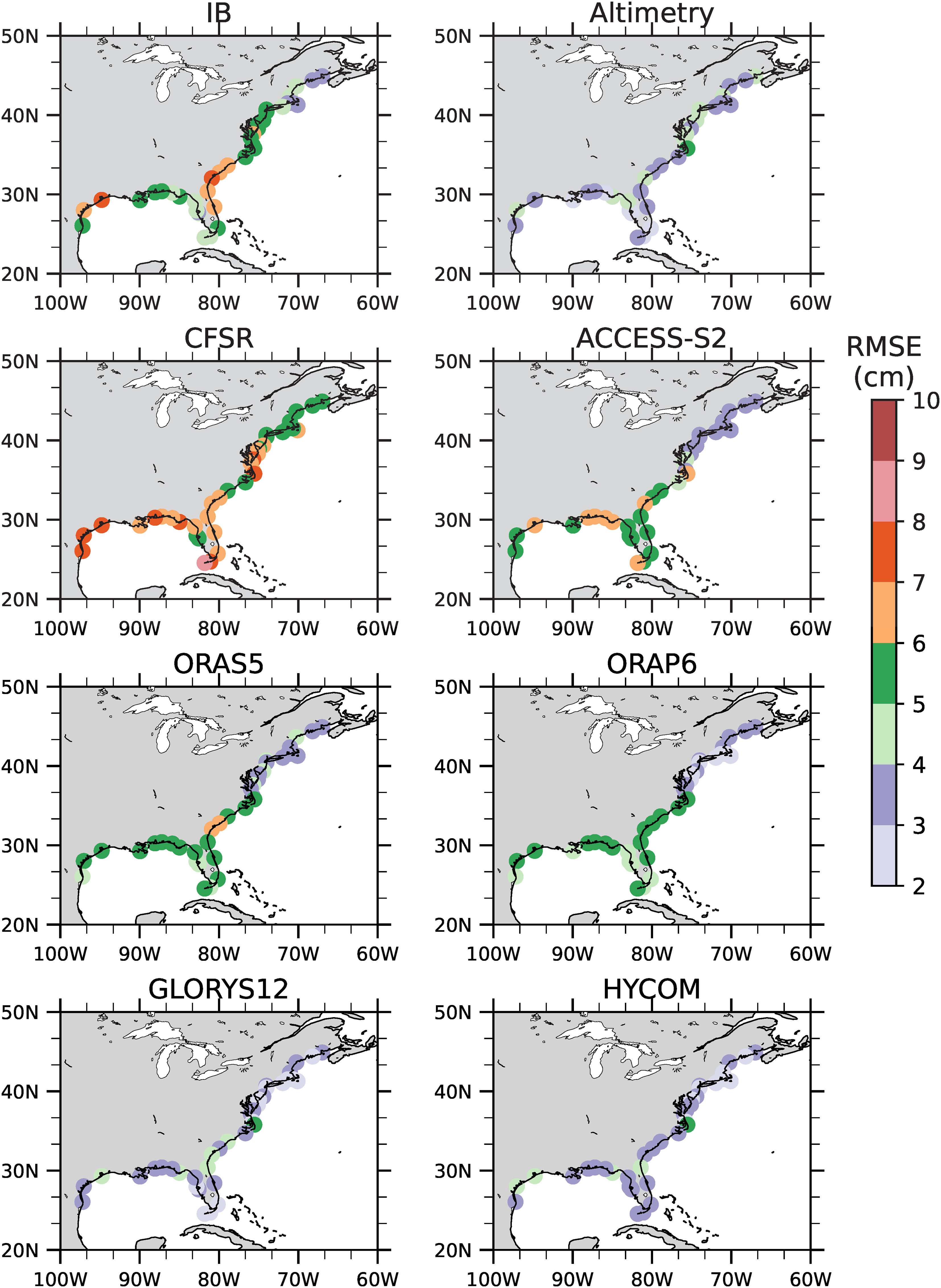
Figure 7 RMSE of tide gauge monthly observations with the IB effect, altimetry, and each of the reanalyses (color bar). Linear trends were removed from the data.

It is also important to note that high-resolution reanalysis products like GLORYS12 and HYCOM demonstrate comparable agreement with tide gauges as altimetry along the Southeast and Gulf Coasts, whereas the much lower-resolution CFSR shows the least skill there (Figures 6, 7). The medium-resolution reanalyses (i.e., those using eddy-permitting models; ACCESS-S2, ORAS5, and ORAP6) show similar spatial patterns, with high ACC (low RMSE) along the Northeast Coast and low ACC (high RMSE) along the Southeast and Gulf Coasts. However, there is a noticeable improvement for ORAP6 compared to ORAS5 at most tide gauge locations. Interestingly, ACCESS-S2 reproduces sea level variability well along the coast, despite not including altimetry assimilation. At a few locations such as in the eastern Gulf of Mexico (e.g., near tide gauges on the Florida West Coast), ACC is lower and RMSE is higher for ACCESS-S2 compared to ORAP6. Overall, according to these performance metrics, reanalyses with the highest resolutions and greatest weight in the assimilation of altimetry (i.e., GLORYS12, HYCOM, and to some extent ORAP6) produce the most realistic representation of coastal sea level variability at tide gauge locations.

We also assessed the temporal characteristics of monthly and annual sea level anomalies at specific locations (Figures 8, 9). At The Battery in New York Harbor, altimetry underestimates monthly variability (Figure 8, left panel; a SD of 3.4 cm compared to 6.0 cm from tide gauge observations), which appears to be partly explained by the absence of IB effect (SD of 2.4 cm). For the CFSR reanalysis, the amount of sea level variability has similar SD values as the tide gauge; however, its ACC is low (0.52) and the RMSE is high (6.0 cm). All other ocean reanalyses exhibit higher ACC and lower RMSE values than CFSR at this location, with GLORYS12 and HYCOM standing out as the most realistic reanalyses compared to this tide gauge (these reanalyses also compare closer than altimetry, again despite also not including the IB effect). On the annual timescale, differences between reanalyses become more pronounced at The Battery (Figure 8, right panels). GLORYS12 has the highest ACC of 0.85 and lowest RMSE of 1.8 cm, followed by ORAP6 (0.81 and 2.0 cm), which outperforms both ORAS5 (0.59 and 2.7 cm) and ACCESS-S2 (0.73 and 2.3 cm).

Figure 8

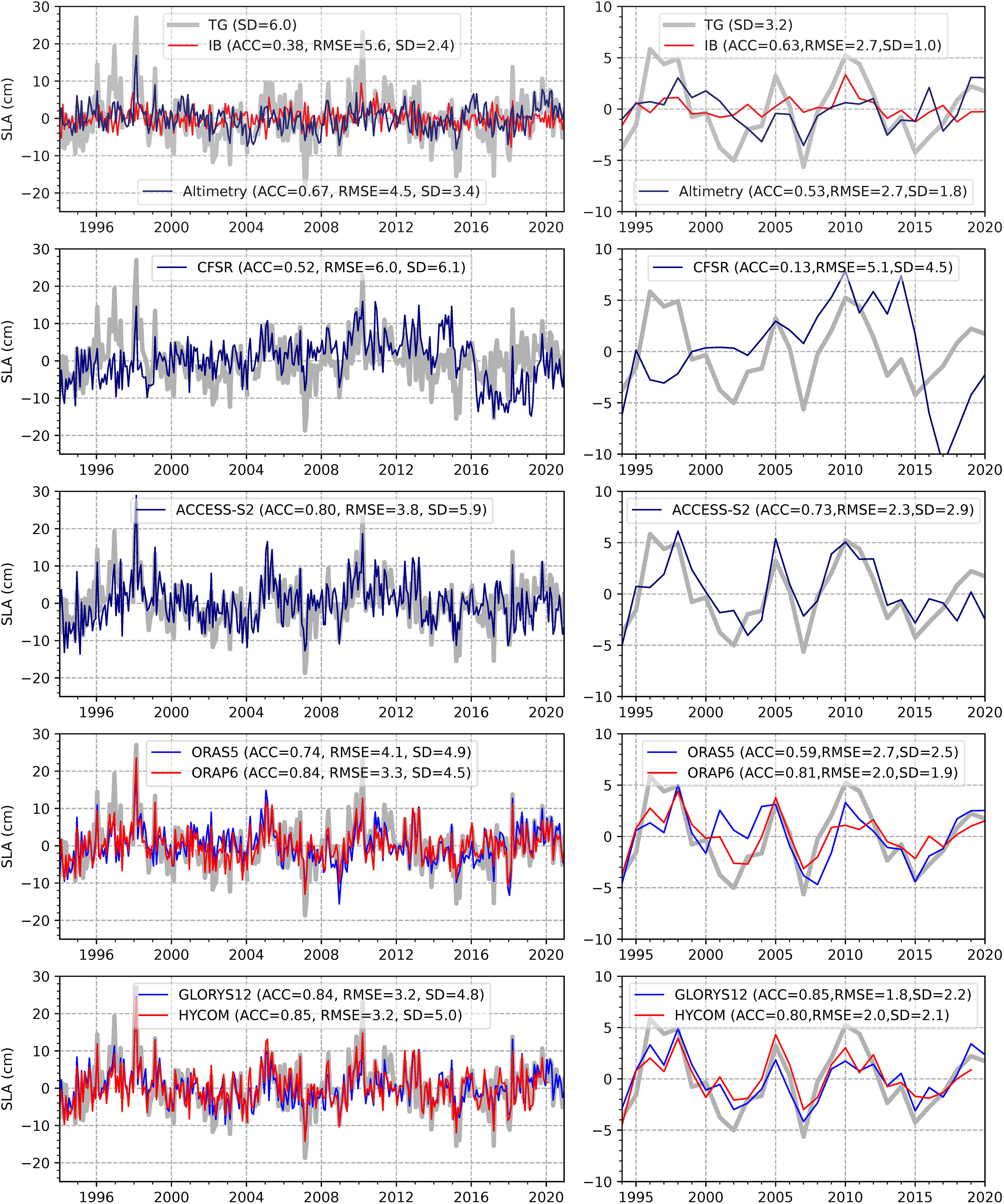
Figure 8 Time series of monthly and annual sea level anomalies at The Battery, NY for each of the observations (tide gauge, IB effect, and altimetry) as well as reanalyses (CFSR, ACCESS-S2, ORAS5, ORAP6, GLORYS12, and HYCOM) as labeled in the legends. Tide gauge observations are shown in all panels (gray lines). Also listed are the SD in cm, ACC, and RMSE in cm. Linear trends were removed from the data.

Figure 9

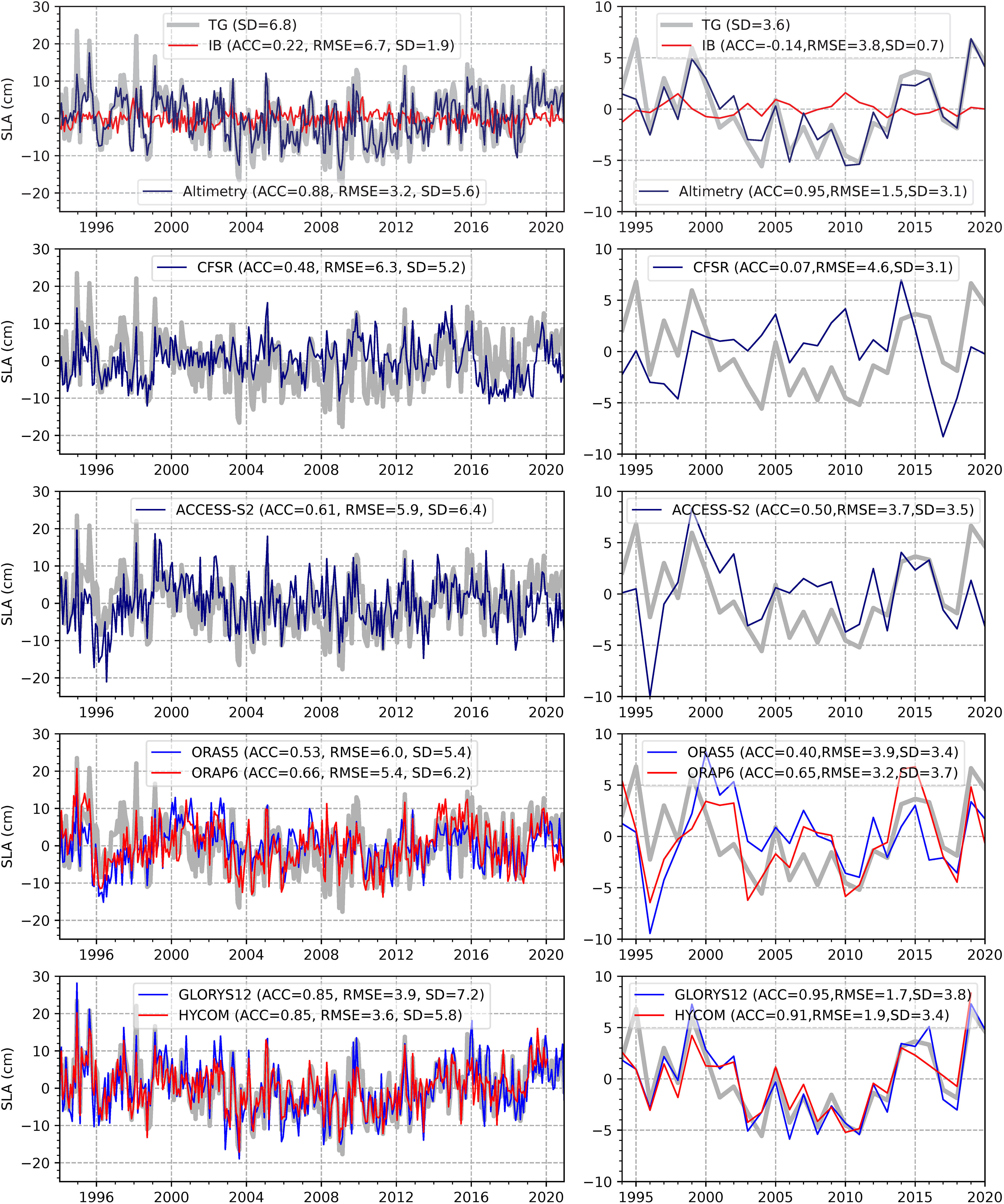
Figure 9 Same as Figure 8, but for Charleston, SC.

At Charleston, sea level variability aligns well between the tide gauge and altimetry observations, exhibiting an ACC of 0.88 on the monthly timescale and 0.95 on the annual timescale (Figure 9, left and right panels, respectively). The IB effect explains less of the tide gauge variability here. GLORYS12 and HYCOM also capture coastal sea level variability at Charleston, especially GLORYS12, which closely matches tide gauge observations on the monthly timescale. On the annual timescale, GLORYS12 performs even better, almost equivalent to altimetry in association with the tide gauge observations. CFSR, however, falls short, demonstrating a very low ACC in the annual mean sea level anomalies (0.07). At Charleston, like at The Battery, according to the ACC and RMSE metrics for the monthly variability, ORAP6 (0.66, 5.4 cm) again outperforms ORAS5 (0.53, 6.0 cm) and ACCESS-S2 (0.61, 5.9 cm). Results are similar at the annual timescale of variability. Additional examples of how the reanalyses perform for Virginia Key and Grand Isle are provided in the Supplementary Materials (Supplementary Figures S4, S5).

Our findings extend to the far southern Southeast and central Gulf Coasts where the results more clearly reveal limitations in eddy-permitting models (i.e., having resolutions of about 1/4°) to accurately simulate coastal sea level variability (Figures 4–7). Problems in the coarser-resolution reanalyses around the Gulf of Mexico emerge, particularly concerning the low-frequency (i.e., annual mean) component of the sea level variability. For example, the annual mean ACC values for ACCESS-S2 are only 0.17 and 0.30 at Virginia Key and Grand Isle, respectively. Reanalyses with altimetry assimilation and eddy-resolving resolution (i.e., 1/12DEGSYMBOL) have better performance around the Gulf of Mexico, as evidenced by higher ACC and lower RMSE values (Figures 4–7). However, the benefit of applying more weight to altimetry in the assimilation, as was done for ORAP6, is less pronounced along the Gulf Coast compared to most of the Southeast Coast. For instance, the annual mean ACC value at Grand Isle improves only marginally from 0.24 in ORAS5 to 0.37 in ORAP6. Similar results for the monthly variability are also seen for the Gulf Coast (e.g., ACC and RMSE values of 0.52 and 5.1 cm for ORAS5 versus 0.56 and 4.9 cm for ORAS6).

3.3 Coastal coherence of variability

Having delineated the role of model resolution, altimetry assimilation, and their limitations in capturing sea level variability on monthly-to-decadal timescales near the coast and at tide gauge locations, specifically, we now turn our attention to the spatial coherence patterns of the temporal variability. The coherence in time and space of coastal sea level variability observed for the East and Gulf Coasts has been widely reported (Thompson and Mitchum, 2014; Woodworth et al., 2014; Piecuch et al., 2016; Calafat et al., 2018). However, an assessment of the coastal coherence in current-generation reanalyses has not been conducted, especially in the context of newly available products with much higher resolution (i.e., GLORYS12 and HYCOM) than previously assessed by Piecuch et al. (2016). We earlier showed that these reanalyses well describe the sea level conditions around individual tide gauges. Here, we utilize the ACC metric with a focus on the spatial pattern of the sea level anomalies associated with monthly-to-decadal variability. We continue using the representative tide gauge locations—The Battery for the Northeast Coast and Charleston for the Southeast Coast—as examples of conditions in the respective regions. Additional insights are provided by similar assessments using Virginia Key and Grand Isle as examples for near and in the Gulf of Mexico (Supplementary Materials). Lastly, we will present a comparative assessment of the coherence of sea level variability between all the tide gauges on the East and Gulf Coasts, thereby taking a new look at how correlated the tide gauges are to each other as well as with altimetry and reanalyses.

Figures 10, 11 show the ACC spatial patterns in altimetry as related to the tide gauges for the Northeast and Southeast Coasts (i.e., considering The Battery and Charleston as the base points, respectively). Sea levels recorded at The Battery are correlated with altimetry throughout the Northeast, with a coherent pattern of ACC in the broad, shallow coastal region less than 500 m deep (Figure 10). The ACC pattern is consistent with descriptions in earlier studies that attribute the coherence near the coast to the dominant role of barotropic processes in the region (Andres et al., 2013; Piecuch et al., 2016). The ACC values diminish rapidly south of Cape Hatteras, indicating that sea levels at this one tide gauge in the Northeast (i.e., The Battery) are not usually related to conditions on the Southeast Coast. Most reanalyses, except for CFSR, capture this coherent pattern well for the Northeast Coast.

Figure 10

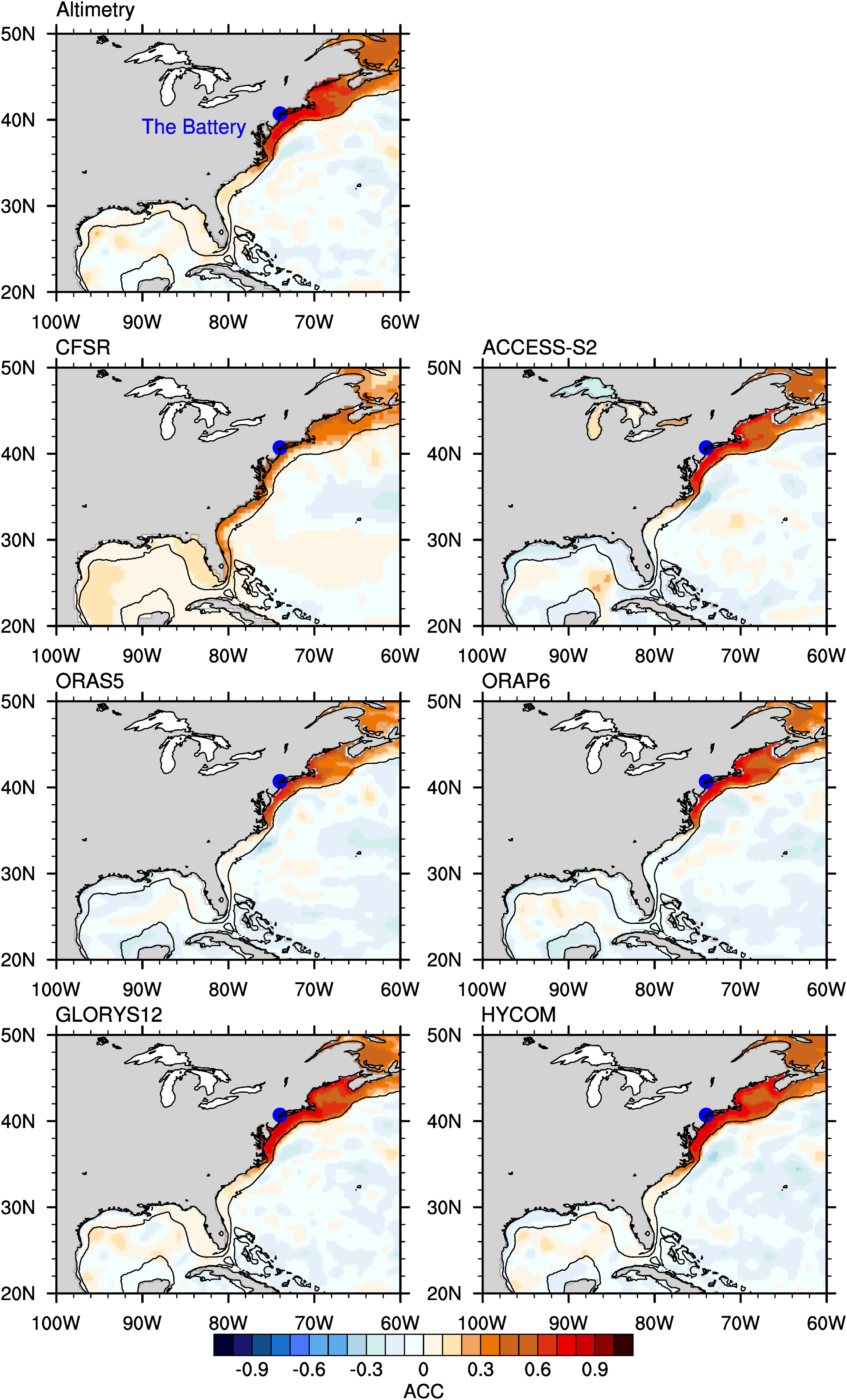
Figure 10 Spatial ACC of monthly sea levels at The Battery (blue dot) from tide gauge observations with altimetry, CFSR, ACCESS-S2, ORAS5, ORAP6, GLORYS12, and HYCOM. Linear trends were removed from the data.

Figure 11

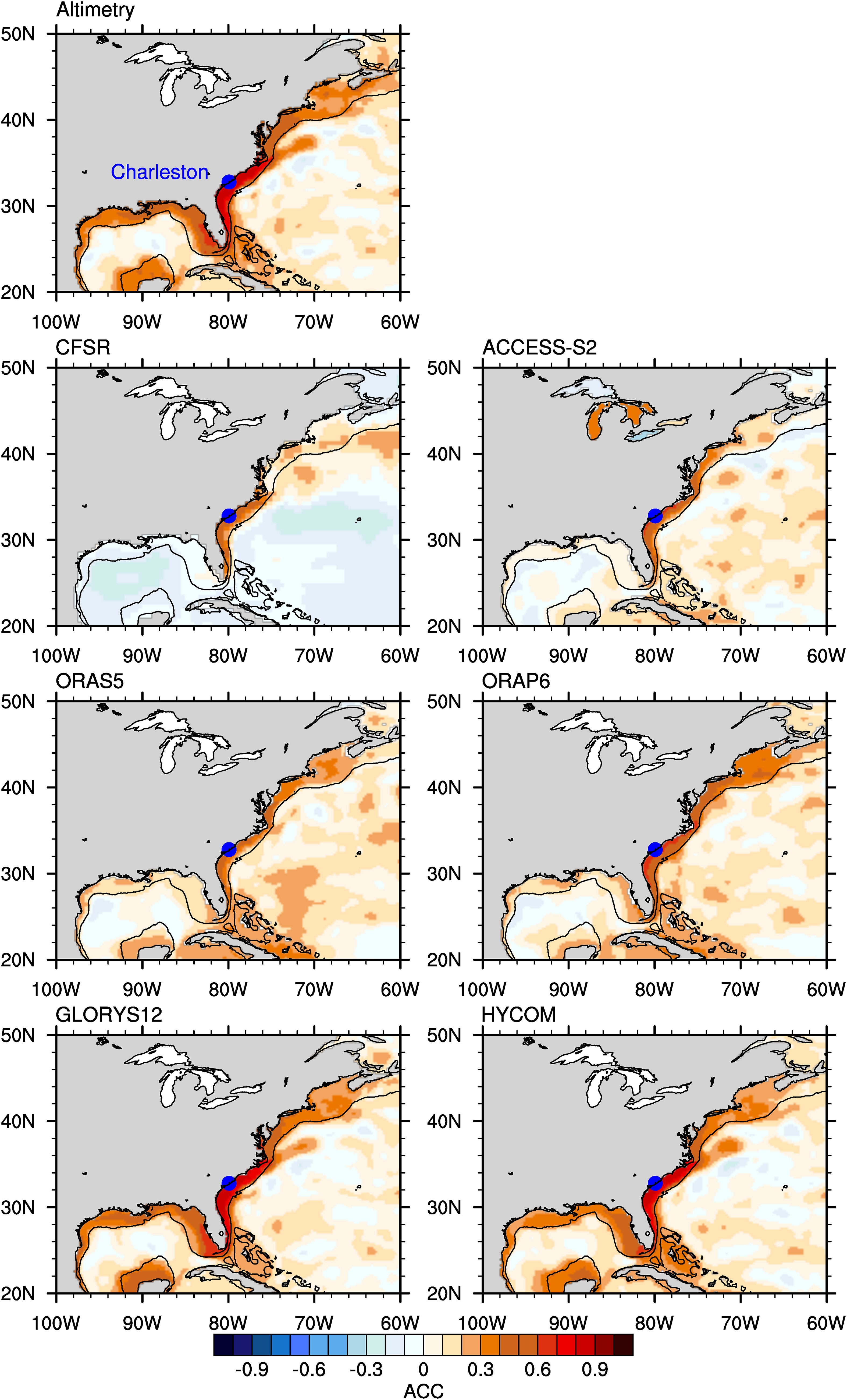
Figure 11 Same as Figure 10, but for Charleston, SC.

The ACC between sea levels at the Charleston tide gauge and altimetry is high along the Southeast Coast, and this correlation also extends into the Gulf of Mexico, though with a reduced magnitude (Figure 11). We see a noteworthy asymmetry in the coastal ACC pattern in that the Charleston tide gauge observations are correlated with monthly sea level anomalies near the Northeast Coast, but not vice versa (i.e., The Battery tide gauge is not strongly correlated with sea levels in the Southeast). Considering the ACC between tide gauges at Virginia Key and Grand Isle with altimetry (Supplementary Figures S6, S7), the coherence patterns are mostly like those seen at Charleston, perceivably due to the similar underlying sea level variability mechanisms (i.e., conversion of offshore planetary wave energy to coastal trapped signals propagating into the Gulf of Mexico; Calafat et al., 2018).

When comparing the reanalyses with altimetry, we find that the coherent pattern over the Northeast Coast is better captured than over the Southeast Coast by most of the models (Figures 10, 11). The eddy-resolving reanalyses (i.e., GLORYS12 and HYCOM) clearly outperform other reanalyses, especially in terms of ACC with the tide gauges at The Battery and Charleston. The reanalyses with lower resolutions (i.e., using eddy-permitting models such as ACCESS-S2, ORAS5, and ORAP6) generally display weaker coherence with both tide gauges, even though the overall spatial pattern mostly agrees with observations. CFSR performs the worst, with its coherent band of correlated sea levels limited to the Southeast Coast and no evidence of coherence along the Gulf Coast. It is promising that the adjustments made for ORAP6 seem to have improved its ACC patterns associated with The Battery and Charleston tide gauges versus what we see for ORAS5 (Figures 10, 11).

We note that the coastal coherence in altimetry observations and the reanalyses is much stronger when using sea levels from the respective products near the tide gauge locations, instead of the actual tide gauge observations, when calculating the ACC (e.g., Supplementary Figures S8, S9 for The Battery and Charleston, respectively). Also, differences between reanalyses in the ACC patterns for this method are smaller compared to if using tide gauge observations as the correlation base points (i.e., as compared to Figures 10, 11 as well as Supplementary Figures S6, S7). For the altimetry observations, the difference using this ACC method is most noticeable for The Battery location (comparing Supplementary Figures S8, 10), which is probably related to the weaker correlations between altimetry and tide gauges in the Northeast (Figure 6). Differences in the ACC patterns based internally or externally to the reanalyses are consistent with results from the multi-model forecasting assessment of Long et al. (2021). For the reanalyses, strong and similar internal correlation patterns are a result of their consistent simulation of ocean dynamic processes affecting sea levels, such as the Gulf Stream, irrespective of how the models actually represent coastal sea level variability observed by tide gauges.

To further understand how the reanalyses depict the coastal coherence of sea levels, we calculated cross-correlations between monthly anomalies at the tide gauge locations on the East and Gulf Coasts. Figure 12 begins by showing the ACC values between each of the 39 tide gauges and themselves. The most coherent signal is found in the Northeast Coast, where ACC values larger than 0.8 cover the area. Tide gauges in the Southeast and Gulf Coasts are also strongly correlated with one another, however, Cape Hatteras marks a sharp separation in the coherence of coastal sea level variability. These results closely match what was shown by Calafat et al. (2018) (cf. their Figure 1).

Figure 12

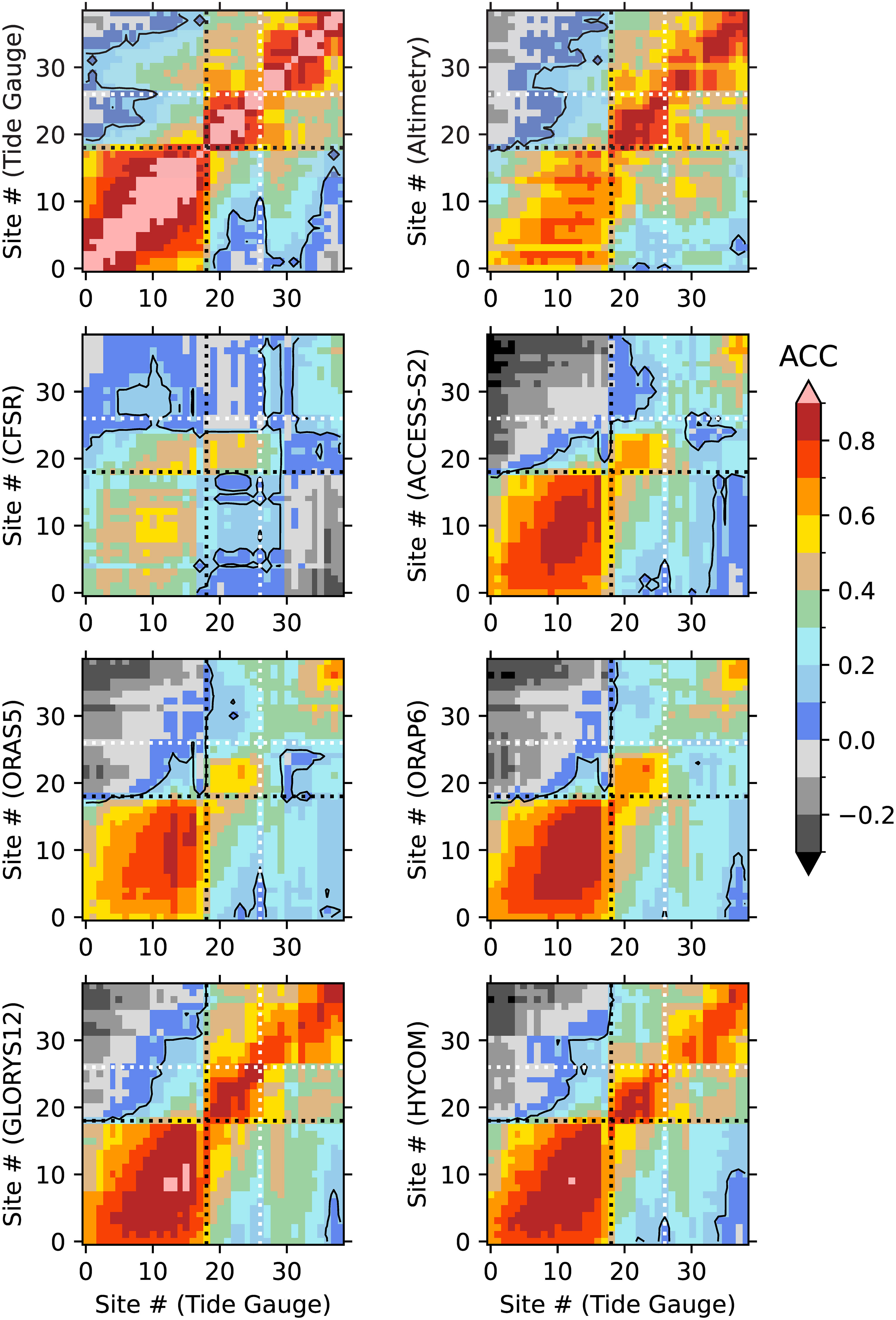
Figure 12 Spatial coherence of ACC (color bar). Tide gauge observations (x-axes) are compared with itself (y-axis; top left panel), altimetry and reanalyses (y-axes; other panels). Site numbers correspond to tide gauges along the East and Gulf Coasts starting in Maine (#0) and following a clockwise direction to Texas (#38). (Supplementary Table S1 lists the tide gauge station names and NOAA identification numbers.) The black (white) dotted lines denote Cape Hatteras (Key West). Black contours enclose non-significant ACC values at the 95% confidence level.

The highest-resolution reanalyses exhibit the best performance in reproducing these patterns of coherence in monthly anomalies (see the y-axis versus x-axis distinction in Figure 12 for GLORYS12 and HYCOM). For the Northeast Coast, the ACC coherence between the tide gauges and GLORYS12 as well as HYCOM is greater than with the altimetry observations. For the Southeast and Gulf Coasts, altimetry is more closely aligned with the tide gauges than is the case for the Northeast Coast, and the reanalyses vary in their performances (listing the coherence patterns from worst to best as compared to what we see for the tide gauges: CFSR, ORAS5, ACCESS-S2, ORAP6, HYCOM, and GLORYS12). Finally, focusing once more on the sea level variability along the Southeast Coast, we see evidence of the improvements that ECMWF made for ORAP6 as compared to ORAS5 (i.e., looking within the area bounded by black and white dotted lines in Figure 12). The best-performing current-generation ocean reanalyses (i.e., HYCOM and GLORYS12) are clearly able to depict the coastal coherence of monthly sea level variability for these parts of the Atlantic Ocean and Gulf of Mexico.

4 Summary and discussion

We evaluated the capability of six global ocean reanalysis products to reproduce monthly sea level variability along the East and Gulf Coasts during the era of near-continuous tide gauge and satellite altimetry observations (1994–2020). In comparing the sea level output from the reanalyses with observations from tide gauges and altimetry, we found substantial improvements in some of the reanalyses in depicting coastal sea level variability, compared to prior-generation reanalyses (Piecuch et al., 2016) as well as seasonal forecast models during the lead-0 month (Long et al., 2021), which have similar conditions as some of the reanalyses (CFSR, ACCESS-S2, and ORAS5). Improvement is particularly large in the two eddy-resolving reanalyses that we assessed (GLORYS12 and HYCOM), although the new assimilation procedure in ORAP6 is also associated with more realistic coastal sea levels, despite it only having eddy-permitting resolution. This section first summarizes our findings on ocean reanalyses and then discusses outstanding questions along with opportunities for enhancement. We will conclude with the implications of accessing global ocean reanalyses that more realistically simulate observed coastal sea level variability.

4.1 Summary

Long-term trends of the tide gauge and altimetry observations show a widespread increase in sea levels for the East and Gulf Coasts, as well as throughout the northwestern Atlantic Ocean (Figure 1). Three of the reanalyses have patterns of sea level rise that resemble the observations (i.e., ORAS5, ORAP6, and GLORYS12), however, the other three reanalyses have substantial differences (i.e., CFSR, ACCESS-S2, and HYCOM). For ACCESS-S2 and HYCOM, most of the trend differences from observations could be addressed by adding global mean sea level rise to the reanalyses. For CFSR, its regional trend bias (i.e., a large downward trend near the Gulf Stream; Figure 1) would make it more difficult to correct a posteriori. The trends in ORAS5 and ORAP6 are much more realistic, although the former reanalysis overestimates the positive trend around the Gulf Stream. This feature is also shared by ACCESS-S2 and is not completely understood. A potential cause of cross-shore gradients in sea level trends, such as those in ACCESS-S2 and ORAS5, is weakening of the Gulf Stream in recent decades (e.g., Piecuch and Beal, 2023). However, the observed weakening of the current would only correspond to cross-shore differences in sea level change of about 1 cm over the period considered here, which is far smaller than the trend biases in ACCESS-S2 and ORAS5. One possibility is that the insufficient resolution in these reanalyses makes variability in the circulation less chaotic and more organized than reality, amplifying long-term circulation changes. The GLORYS12 reanalysis, with its inclusion of global mean sea level rise and eddy-permitting resolution, has the most similar trend to observations, at least in the open ocean. Near the coast, however, the trends in GLORYS12 are smaller compared to the tide gauge observations, which can be explained at least for the western Gulf of Mexico by the effect of land subsidence that is unresolved by all the reanalyses.

High-tide flooding is increasing due to sea level rise, and variability on monthly-to-decadal timescales affects the occurrence and severity of impacts (Dusek et al., 2022; Volkov et al., 2023). The annual cycle is the largest mode of sea level variability for much of the northwestern Atlantic Ocean (e.g., Widlansky et al., 2020), especially near the East and Gulf Coasts (Figure 2). All reanalyses that we assessed capture the observed spatial pattern, range, and phasing of the annual cycle, both near the coast and offshore. We only noted subtle biases of the annual cycles in some of the reanalyses (e.g., in CFSR, the coastal variability is too large north of Cape Hatteras), which ideally should be addressed as any problems in the climatology will ultimately degrade the realism of monthly anomalies.

Monthly sea level anomalies are associated with much of the high-tide flooding that impacts the U.S. Coast (e.g., Dusek et al., 2022). While the greatest sea level variability is observed by altimetry to be in the offshore regions, especially around the Gulf Stream and Loop Current System, there is also substantial variability nearshore (i.e., SD values greater than 5 cm; Figure 3). Most of the tide gauges on the Southeast and the western Gulf Coasts indicate a similar amount of variability (Figure 3).

For the assessment of sea level variability, overall, we found the resemblance of reanalyses to observations to be greatest for GLORYS12 and smallest for CFSR, according to the SD patterns (Figure 3) as well as the ACC and RMSE metrics of temporal variability (Figures 4–9). We were somewhat surprised by how closely the monthly sea level anomalies in GLORYS12 aligned with most of the tide gauges (e.g., its ACC for Charleston is 0.85; see also Supplementary Table S2; Figure 6). The spatial coherence of coastal variability in the GLORYS12 reanalysis also most closely matched the observed pattern of strong correlations between tide gauges and regional altimetry anomalies (Figures 10–12). HYCOM performs nearly as well as GLORYS12 according to these metrics (e.g., its ACC at Charleston is also 0.85), whereas there are some deficiencies in each of the ACCESS-S2, ORAS5, and ORAP6 reanalyses especially for the Southeast Coast (e.g., the respective ACC values at Charleston are 0.61, 0.53, and 0.66). The CFSR performance was worst overall, although its ACC value at Charleston (0.48) is not much lower than ORAS5.

In assessing annual mean anomalies of the reanalyses, a much larger deficiency in CFSR is evident (Figures 8, 9). CFSR has only a 0.07 ACC with the Charleston tide gauge at the annual timescale. Piecuch et al. (2016) showed similar problems in annual mean sea level variability for some prior-generation ocean reanalyses. We also found degraded performance at the annual timescale, compared to monthly variability, for the ACCESS-S2 and ORAS5 reanalyses (ACC values of 0.50 and 0.40, respectively, at Charleston). The other three reanalyses (ORAP6, HYCOM, and GLORYS12) had similar or higher ACC values at the annual timescale compared to their performances for monthly variability. Again, GLORYS12 is the best-performing reanalysis for the locations we assessed (e.g., having annual mean ACC values of 0.85 and 0.95 for The Battery and Charleston, respectively; Figures 8, 9). The strong performance at the annual timescale of GLORYS12 as well as HYCOM, and to some extent also ORAP6, is evidence of a clear improvement over prior-generation capabilities analysing coastal sea level variability on annual timescales (Piecuch et al., 2016).

The results suggest that reanalyses with similar horizontal resolutions generally exhibit comparable skill levels in simulating sea level variations along the East and Gulf Coasts. While the skill levels can be grouped to some extent by the horizontal resolution of the ocean models used in these reanalyses, it is important to note that the sensitivity of sea levels to model resolution varies along different coastal regions. Specifically, sea levels near the Northeast Coast appear less sensitive to model resolution than those around the Southeast and Gulf Coasts. In the Northeast, the ACC for ACCESS-S2, ORAS5, and ORAP6 with altimetry ranges from 0.6–0.8, only marginally weaker than that of GLORYS12 and HYCOM, which ranges from 0.7–0.9 (Figure 4). At a few tide gauges between The Battery and Cape Hatteras, such as Atlantic City (New Jersey), ACCESS-S2 and ORAP6 achieve an ACC exceeding 0.8, which is comparable to that of GLORYS12 and HYCOM (Figure 6; see also Supplementary Table S2). Furthermore, the sea level coherence pattern for the Northeast Coast is nearly as accurately reproduced in ACCESS-S2, ORAS5, and ORAP6 as in GLORYS12 and HYCOM (Figure 10). The Southeast and Gulf Coasts show a more pronounced ACC difference between eddy-permitting and eddy-resolving reanalyses. For instance, eddy-resolving reanalyses like GLORYS12 and HYCOM typically show much higher correlations with tide gauge records (ACC values usually above 0.8) than do eddy-permitting reanalyses like ACCESS-S2, ORAS5, and ORAP6 (each with an ACC of around 0.6).

4.2 Interpretation and implications

Regional differences in the sensitivity of the reanalysis performances to horizontal resolution may be attributable to the dominant physical processes in each area. Previous studies suggest that along the Northeast Coast, sea level variability is associated with barotropic processes forced by alongshore wind stresses (Andres et al., 2013; Piecuch et al., 2016; Zhu et al., 2024). Such oceanic processes are not dependent on model resolution, at least for the 1/2° or finer grids considered here. Conversely, accurate simulation of the Gulf Stream and Loop Current—key drivers of sea level variability along the Southeast and Gulf Coasts—requires higher model resolution (Li et al., 2022a). Furthermore, model resolution can impact how well sea level variations are captured depending on whether bathymetry is adequately resolved. For example, oceanic Rossby waves can influence sea levels along the Southeast Coast (Hong et al., 2000; Dangendorf et al., 2023; Zhu et al., 2024), and then into the Gulf of Mexico by coastal-trapped waves passing through the narrow Florida Strait (Calafat et al., 2018). Given that the continental slope affects coastal wave characteristics, and the narrow strait influences wave energy entering the Gulf of Mexico, it is essential for models to have sufficient resolution to capture these bathymetric features accurately. Among the reanalyses assessed, CFSR had the worst performance, which may be attributed to its lower model resolution and associated inadequacies in simulating the Gulf Stream, or potential issues in the assimilation of ocean observations (Long et al., 2021).

In addition to model resolution, assimilation of altimetry and other ocean observations impact the sea level simulation in the reanalyses. For instance, ORAP6, which incorporates altimetry observations with more weight during the assimilation, demonstrates better performance in capturing monthly sea level fluctuations along the Southeast Coast compared to its predecessor, ORAS5 (Figures 4, 5). The latter reanalysis did not assimilate ocean observations in regions shallower than 500 m. In the absence of altimetry assimilation, ACCESS-S2’s performance is like that of ORAS5, but not as good as ORAP6, at most of the tide gauge locations along the East Coast (Figures 6, 7). Interestingly, the benefits of altimetry assimilation are less pronounced in the Gulf of Mexico for reanalyses at a 1/4° resolution, possibly due to unresolved physical processes in these models. The most substantial improvements for the Gulf Coast and everywhere else are in the higher-resolution 1/12° reanalyses, specifically GLORYS12 and HYCOM, which also have sophisticated assimilation systems that include altimetry.

Overall, our findings suggest an association between more accurate reanalyses and the use of higher-resolution ocean models along with robust data assimilation, at least as far as their ability to represent coastal sea level variability when compared to tide gauge and altimetry observations. While enhancing the weighting of observational data in the assimilation process appears to improve reanalyses of sea level (e.g., as was done for ORAP6), future research is needed to assess its implications for sea level forecasting as well as describing other ocean variables in reanalyses.

This study underscores the advancements in modelling techniques for accurately capturing observed sea level variability along coastal regions. We attribute the improvements in certain reanalyses to a combination of enhanced spatial resolutions and more effective assimilation of ocean observations, including satellite altimetry data. Among the best-performing reanalyses—GLORYS12 and HYCOM—we find instances where their fidelity to tide gauge observations surpasses even the altimetry products considered in this study (cf. Figures 6, 7). One notable example is the comparison with the tide gauge at The Battery where the GLORYS12 and HYCOM reanalyses outperform altimetry in capturing coastal sea level variability (Figure 8). This suggests that the dynamical processes modelled in these reanalyses offer insights beyond what can be achieved through objective analyses based solely on observations, like the gridded altimetry product we assessed. Further improvement in the realism of the reanalyses could be attained by including the IB effect on sea level (Piecuch and Ponte, 2015), such as by adding atmospheric surface pressure information to the ocean model output (cf. Figure 8 especially). Importantly, none of the reanalyses incorporate tide gauge observations, raising the question of whether such assimilation could yield even more accurate coastal sea level simulations.

High-quality ocean reanalyses are indispensable for advancing our understanding of coastal sea level variability and its ongoing changes. Given growing concern around sea level rise, the need for reliable coastal information is more pressing than ever, especially for forecasting sea level changes and assessing their potential societal impacts. This study contributes to the broader effort of enhancing our understanding of coastal sea levels, with the aim of improving both monitoring and forecasting systems, which has implications for coastal management and climate adaptation strategies. Our results highlight the necessity for further research to explore the causes of varying performance among different reanalyses. Moreover, this study prompts the development of innovative ocean reanalysis methods, such as incorporating tide gauge observations. Improving sea level forecasts is an urgent need for many coastal communities (Dusek et al., 2022), and enhanced ocean analyses could be a pivotal first step toward more skilful outlooks. While our study is focused on the East and Gulf Coasts, the insights gained are applicable to other coastal regions worldwide, which are similarly grappling with the challenges posed by sea level rise and extreme events.

Data availability statement

Tide gauge observations are available from the NOAA Tides and Currents Archive via the CO-OPS Data Retrieval API (https://api.tidesandcurrents.noaa.gov/api/prod/). Altimetry observations and the GLORYS12 reanalysis are available from the E.U. Copernicus Marine Service (https://data.marine.copernicus.eu/product/SEALEVEL_GLO_PHY_CLIMATE_L4_MY_008_057/ and https://data.marine.copernicus.eu/product/GLOBAL_MULTIYEAR_PHY_001_030/, respectively). The remaining reanalyses are available from the following sources: CFSR (https://www.ncei.noaa.gov/products/weather-climate-models/climate-forecast-system), ACCESS-S2 (https://dapds00.nci.org.au/thredds/catalogs/ux62/access-s2/access-s2.html), ORAS5 (https://cds.climate.copernicus.eu/), ORAP6 (forthcoming), and HYCOM (https://www.hycom.org/dataserver/gofs-3pt1/analysis). The DAC dataset used to calculate the IB effect is available from AVISO (https://www.aviso.altimetry.fr/en/data/products/auxiliary-products/dynamic-atmospheric-correction.html). Further inquiries can be directed to the corresponding authors.

Author contributions

XF: Conceptualization, Data curation, Formal analysis, Investigation, Methodology, Software, Visualization, Writing – original draft, Writing – review & editing. MW: Conceptualization, Funding acquisition, Methodology, Project administration, Resources, Supervision, Writing – original draft, Writing – review & editing. MB: Data curation, Methodology, Writing – review & editing. HZ: Data curation, Methodology, Writing – review & editing. CS: Data curation, Methodology, Writing – review & editing. GS: Methodology, Writing – review & editing. XL: Methodology, Writing – review & editing. PT: Methodology, Writing – review & editing. AK: Methodology, Writing – review & editing. GD: Methodology, Writing – review & editing. WS: Methodology, Writing – review & editing.

Funding

The author(s) declare financial support was received for the research, authorship, and/or publication of this article. This study was primarily supported by the NOAA Climate Program Office’s Modelling, Analysis, Predictions, and Projections (MAPP) program through grant NA22OAR4310138.

Acknowledgments

The authors thank the climate monitoring and prediction centres for making available their reanalyses. A large-language model (GPT4 from OpenAI) was used to organize and clarify the writing.

Conflict of interest

The authors declare that the research was conducted in the absence of any commercial or financial relationships that could be construed as a potential conflict of interest.

Publisher’s note

All claims expressed in this article are solely those of the authors and do not necessarily represent those of their affiliated organizations, or those of the publisher, the editors and the reviewers. Any product that may be evaluated in this article, or claim that may be made by its manufacturer, is not guaranteed or endorsed by the publisher.

Supplementary material

The Supplementary Material for this article can be found online at: https://www.frontiersin.org/articles/10.3389/fmars.2024.1338626/full#supplementary-material

References

Andres M., Gawarkiewicz G. G., Toole J. M. (2013). Interannual sea level variability in the western North Atlantic: Regional forcing and remote response. Geophys. Res. Lett. 40, 5915–5919. doi: 10.1002/2013GL058013

CrossRef Full Text | Google Scholar

Balmaseda M. A., Mogensen K., Weaver A. T. (2013). Evaluation of the ECMWF ocean reanalysis system ORAS4. Q. J. R. Meteorol. Soc 139, 1132–1161. doi: 10.1002/qj.2063

CrossRef Full Text | Google Scholar

Calafat F. M., Wahl T., Lindsten F., Williams J., Frajka-Williams E. (2018). Coherent modulation of the sea-level annual cycle in the United States by Atlantic Rossby waves. Nat. Commun. 9, 2571. doi: 10.1038/s41467-018-04898-y

PubMed Abstract | CrossRef Full Text | Google Scholar

Chi L., Wolfe C. L. P., Hameed S. (2018). Intercomparison of the Gulf Stream in ocean reanalyses: 1993–2010. Ocean Model. 125, 1–21. doi: 10.1016/j.ocemod.2018.02.008

CrossRef Full Text | Google Scholar

Dangendorf S., Hendricks N., Sun Q., Klinck J., Ezer T., Frederikse T., et al. (2023). Acceleration of U.S. Southeast and Gulf coast sea-level rise amplified by internal climate variability. Nat. Commun. 14, 1935. doi: 10.1038/s41467-023-37649-9

PubMed Abstract | CrossRef Full Text | Google Scholar

Dusek G., Sweet W. V., Widlansky M. J., Thompson P. R., Marra J. J. (2022). A novel statistical approach to predict seasonal high tide flooding. Front. Mar. Sci. 9. doi: 10.3389/fmars.2022.1073792

PubMed Abstract | CrossRef Full Text | Google Scholar

Harvey T. C., Hamlington B. D., Frederikse T., Nerem R. S., Piecuch C. G., Hammond W. C., et al. (2021). Ocean mass, sterodynamic effects, and vertical land motion largely explain US coast relative sea level rise. Commun. Earth Environ. 2. doi: 10.1038/s43247-021-00300-w

CrossRef Full Text | Google Scholar

Hodson T. O. (2022). Root-mean-square error (RMSE) or mean absolute error (MAE): when to use them or not. Geosci Model. Dev. 15, 5481–5487. doi: 10.5194/gmd-15-5481-2022

CrossRef Full Text | Google Scholar

Hong B. G., Sturges W., Clarke A. J. (2000). Sea level on the U.S. East Coast: Decadal variability caused by open ocean wind-curl forcing. J. Phys. Oceanogr. 30, 2088–2098. doi: 10.1175/1520-0485(2000)030<2088:SLOTUS>2.0.CO;2

CrossRef Full Text | Google Scholar

Jean-Michel L., Eric G., Romain B.-B., Gilles G., Angélique M., Marie D., et al. (2021). The copernicus global 1/12° Oceanic and sea ice GLORYS12 reanalysis. Front. Earth Sci. 9. doi: 10.3389/feart.2021.698876

CrossRef Full Text | Google Scholar

Kleinosky L. R., Yarnal B., Fisher A. (2007). Vulnerability of hampton roads, virginia to storm-surge flooding and sea-level rise. Nat. Hazards 40, 43–70. doi: 10.1007/s11069-006-0004-z

CrossRef Full Text | Google Scholar

Kolker A. S., Allison M. A., Hameed S. (2011). An evaluation of subsidence rates and sea-level variability in the northern Gulf of Mexico. Geophys. Res. Lett. 38. doi: 10.1029/2011GL049458

CrossRef Full Text | Google Scholar

Li D., Chang P., Yeager S. G., Danabasoglu G., Castruccio F. S., Small J., et al. (2022a). The impact of horizontal resolution on projected sea-level rise along US east continental shelf with the community earth system model. J. Adv. Model. Earth Syst. 14. doi: 10.1029/2021MS002868

PubMed Abstract | CrossRef Full Text | Google Scholar

Li S., Wahl T., Barroso A., Coats S., Dangendorf S., Piecuch C., et al. (2022b). Contributions of different sea-level processes to high-tide flooding along the U.S. Coastline. J. Geophys. Res. Ocean. 127, e2021JC018276. doi: 10.1029/2021JC018276

CrossRef Full Text | Google Scholar

Liu Y., Li J., Fasullo J., Galloway D. L. (2020). Land subsidence contributions to relative sea level rise at tide gauge Galveston Pier 21, Texas. Sci. Rep. 10, 17905. doi: 10.1038/s41598-020-74696-4

PubMed Abstract | CrossRef Full Text | Google Scholar

Long X., Widlansky M. J., Spillman C. M., Kumar A., Balmaseda M., Thompson P. R., et al. (2021). Seasonal forecasting skill of sea-level anomalies in a multi-model prediction framework. J. Geophys. Res. Ocean. 126, e2020JC017060. doi: 10.1029/2020JC017060

CrossRef Full Text | Google Scholar

Metzger E. J., Smedstad O. M., Thoppil P., Hurlburt H., Cummings J., Walcraft A., et al. (2014). US navy operational global ocean and arctic ice prediction systems. Oceanography 27, 32–43. doi: 10.5670/oceanog.2014.66

CrossRef Full Text | Google Scholar

Moftakhari H. R., AghaKouchak A., Sanders B. F., Matthew R. A. (2017). Cumulative hazard: The case of nuisance flooding. Earth’s Futur. 5, 214–223. doi: 10.1002/2016EF000494

CrossRef Full Text | Google Scholar

Piecuch C. G., Beal L. M. (2023). Robust weakening of the Gulf Stream during the past four decades observed in the Florida Straits. Geophys. Res. Lett. 50. doi: 10.1029/2023GL105170

CrossRef Full Text | Google Scholar

Piecuch C. G., Dangendorf S., Ponte R. M., Marcos M. (2016). Annual sea level changes on the North American northeast coast: influence of local winds and barotropic motions. J. Clim. 29, 4801–4816. doi: 10.1175/JCLI-D-16-0048.1

CrossRef Full Text | Google Scholar

Piecuch C. G., Ponte R. M. (2015). Inverted barometer contributions to recent sea level changes along the northeast coast of North America. Geophys. Res. Lett. 42, 5918–5925. doi: 10.1002/2015GL064580

CrossRef Full Text | Google Scholar

Ray R. D., Widlansky M. J., Genz A. S., Thompson P. R. (2023). Offsets in tide-gauge reference levels detected by satellite altimetry: Ten case studies. J. Geod. 97. doi: 10.1007/s00190-023-01800-7

PubMed Abstract | CrossRef Full Text | Google Scholar

Saha S., Moorthi S., Pan H.-L., Wu X., Wang J., Nadiga S., et al. (2010). The NCEP climate forecast system reanalysis. Bull. Am. Meteorol. Soc 91, 1015–1058. doi: 10.1175/2010BAMS3001.1

CrossRef Full Text | Google Scholar

Saha S., Moorthi S., Wu X., Wang J., Nadiga S., Tripp P., et al. (2014). The NCEP climate forecast system version 2. J. Clim. 27, 2185–2208. doi: 10.1175/JCLI-D-12-00823.1

CrossRef Full Text | Google Scholar

Sallenger A. H., Doran K. S., Howd P. A. (2012). Hotspot of accelerated sea-level rise on the Atlantic coast of North America. Nat. Clim. Change 2, 884–888. doi: 10.1038/nclimate1597

CrossRef Full Text | Google Scholar

Stammer D., Cazenave A., Ponte R. M., Tamisiea M. E. (2013). Causes for contemporary regional sea level changes. Ann. Rev. Mar. Sci. 5, 21–46. doi: 10.1146/annurev-marine-121211-172406

PubMed Abstract | CrossRef Full Text | Google Scholar

Stephens S. A., Bell R. G., Lawrence J. (2018). Developing signals to trigger adaptation to sea-level rise. Environ. Res. Lett. 13. doi: 10.1088/1748-9326/aadf96

CrossRef Full Text | Google Scholar

Sweet W. V., Dusek G., Obeysekera J., Marra J. (2018). Patterns and projections of high tide flooding along the U.S. coastline using a common impact threshold. NOAA Technical Report NOS CO-OPS 086 (Silver Spring, MD: National Oceanic and Atmospheric Administration, National Ocean Service), 44 pp. doi: 10.7289/V5/TR-NOS-COOPS-086

CrossRef Full Text | Google Scholar

Sweet W. V., Hamlington B. D., Kopp R. E., Weaver C. P., Barnard P. L., Bekaert D., et al. (2022). Global and Regional Sea Level Rise Scenarios for the United States: Updated Mean Projections and Extreme Water Level Probabilities Along U.S. Coastlines. NOAA Technical Report NOS 01 (Silver Spring, MD: National Oceanic and Atmospheric Administration, National Ocean Service), 111 pp.

Google Scholar

Sweet W. V., Park J. (2014). From the extreme to the mean: Acceleration and tipping points of coastal inundation from sea level rise. Earth’s Futur. 2, 579–600. doi: 10.1002/2014EF000272

CrossRef Full Text | Google Scholar

Thompson P. R., Mitchum G. T. (2014). Coherent sea level variability on the North Atlantic western boundary. J. Geophys. Res. Ocean. 119, 5676–5689. doi: 10.1002/2014JC009999

CrossRef Full Text | Google Scholar

Thompson P. R., Widlansky M. J., Hamlington B. D., Merrifield M. A., Marra J. J., Mitchum G. T., et al. (2021). Rapid increases and extreme months in projections of United States high-tide flooding. Nat. Clim. Change 11, 584–590. doi: 10.1038/s41558-021-01077-8

CrossRef Full Text | Google Scholar

Valle-Levinson A., Dutton A., Martin J. B. (2017). Spatial and temporal variability of sea level rise hot spots over the eastern United States. Geophys. Res. Lett. 44, 7876–7882. doi: 10.1002/2017GL073926

CrossRef Full Text | Google Scholar

Vitousek S., Barnard P. L., Fletcher C. H., Frazer N., Erikson L., Storlazzi C. D. (2017). Doubling of coastal flooding frequency within decades due to sea-level rise. Sci. Rep. 7, 1399. doi: 10.1038/s41598-017-01362-7

PubMed Abstract | CrossRef Full Text | Google Scholar

Volkov D. L., Zhang K., Johns W. E., Willis J. K., Hobbs W., Goes M., et al. (2023). Atlantic meridional overturning circulation increases flood risk along the United States southeast coast. Nat. Commun. 14. doi: 10.1038/s41467-023-40848-z

CrossRef Full Text | Google Scholar

Wahl T., Jain S., Bender J., Meyers S. D., Luther M. E. (2015). Increasing risk of compound flooding from storm surge and rainfall for major US cities. Nat. Clim. Change 5, 1093–1097. doi: 10.1038/nclimate2736

CrossRef Full Text | Google Scholar

Wdowinski S., Bray R., Kirtman B. P., Wu Z. (2016). Increasing flooding hazard in coastal communities due to rising sea level: Case study of Miami Beach, Florida. Ocean Coast. Manage. 126, 1–8. doi: 10.1016/j.ocecoaman.2016.03.002

CrossRef Full Text | Google Scholar

Wedd R., Alves O., de Burgh-Day C., Down C., Griffiths M., Hendon H. H., et al. (2022). ACCESS-S2: the upgraded Bureau of Meteorology multi-week to seasonal prediction system. J. South. Hemisph. Earth Syst. Sci. 72, 218–242. doi: 10.1071/ES22026

CrossRef Full Text | Google Scholar

Widlansky M. J., Long X., Balmaseda M. A., Spillman C. M., Smith G., Zuo H., et al. (2023). Quantifying the benefits of altimetry assimilation in seasonal forecasts of the upper ocean. J. Geophys. Res. Ocean. 128. doi: 10.1029/2022JC019342

CrossRef Full Text | Google Scholar

Widlansky M. J., Long X., Schloesser F. (2020). Increase in sea level variability with ocean warming associated with the nonlinear thermal expansion of seawater. Commun. Earth Environ. 1, 9. doi: 10.1038/s43247-020-0008-8

CrossRef Full Text | Google Scholar

Widlansky M. J., Marra J. J., Chowdhury M. R., Stephens S. A., Miles E. R., Fauchereau N., et al. (2017). Multimodel ensemble sea level forecasts for tropical Pacific Islands. J. Appl. Meteorol. Climatol. 56, 849–862. doi: 10.1175/JAMC-D-16-0284.1

CrossRef Full Text | Google Scholar

Woodworth P. L., Maqueda M. Á.M., Roussenov V. M., Williams R. G., Hughes C. W. (2014). Mean sea-level variability along the northeast American Atlantic coast and the roles of the wind and the overturning circulation. J. Geophys. Res. Ocean. 119, 8916–8935. doi: 10.1002/2014JC010520

CrossRef Full Text | Google Scholar

Wöppelmann G., Marcos M. (2016). Vertical land motion as a key to understanding sea level change and variability. Rev. Geophys. 54, 64–92. doi: 10.1002/2015RG000502

CrossRef Full Text | Google Scholar

Yin J., Schlesinger M. E., Stouffer R. J. (2009). Model projections of rapid sea-level rise on the northeast coast of the United States. Nat. Geosci. 2, 262–266. doi: 10.1038/ngeo462

CrossRef Full Text | Google Scholar

Zhu Y., Han W., Alexander M. A., Shin S.-I. (2024). Interannual sea level variability along the U.S. East coast during satellite altimetry era: local versus remote forcing. J. Clim. 37, 21–39 doi: 10.1175/JCLI-D-23-0065.1

CrossRef Full Text | Google Scholar

Zuo H., Alonso Balmaseda M., de Boisseson E., Tietsche S., Mayer M., de Rosnay P. (2021). The ORAP6 ocean and sea-ice reanalysis: description and evaluation. (EGU General Assembly 2021), EGU21–E9997. doi: 10.5194/egusphere-egu21-9997

CrossRef Full Text | Google Scholar

Zuo H., Balmaseda M. A., Tietsche S., Mogensen K., Mayer M. (2019). The ECMWF operational ensemble reanalysis–analysis system for ocean and sea ice: a description of the system and assessment. Ocean Sci. 15, 779–808. doi: 10.5194/os-15-779-2019

CrossRef Full Text | Google Scholar