Seasonal variability of coastal pH and CO2 using an oceanographic buoy in the Canary Islands

Ocean acidification, caused by the absorption of carbon dioxide (CO₂) from the atmosphere into the ocean, ranks among the most critical consequences of climate change for marine ecosystems. Most studies have examined pH and CO₂ trends in the open ocean through oceanic time-series research. The analysis in coastal waters, particularly in island environments, remains relatively underexplored. This gap in our understanding is particularly important given the profound implications of these changes for coastal ecosystems and the blue economy. The present study focuses on the ongoing monitoring effort that started in March 2020 along the east coast of Gran Canaria, within the Gando Bay, by the CanOA-1 buoy. This monitoring initiative focuses on the systematic collection of multiple variables within the CO₂ system, such as CO₂ fugacity (fCO₂), pH (in total scale, pH_T), total inorganic carbon (C_T), and other hydrographic variables including sea surface salinity (SSS), sea surface temperature (SST) and wind intensity and direction. Accordingly, the study allows the computation of the CO₂ flux (FCO₂) between the surface waters and the atmosphere. During the study period, stational (warm and cold periods) behavior was found for all the variables. The lowest SST values were recorded in March, with a range of 18.8-19.3°C, while the highest SST were observed in September and October, ranging from 24.5-24.8°C. SST exhibited an annual increase with a rate of 0.007°C yr^-1. Warmer months increased SSS, while colder periods, influenced by extreme events like tropical storms, led to lower salinity (SSS=34.02). The predominant Trade Winds facilitated the arrival of deeper water, replenishing seawater. The study provided insights into atmospheric CO₂. Atmospheric fCO₂ averaged 415 ± 4 µatm (2020-2023). Surface water fCO_2sw presented variability, with the highest values recorded in September and October, peaking at 437 µatm in September 2021. The lowest values for fCO_2sw were found in February 2021 (368 µatm). From 2020 to 2023, surface water fCO_2sw values displayed an increasing rate of 1.9 µatm yr^-1 in the study area. The assessment of fCO_2sw decomposition into thermal and non-thermal processes revealed the importance of SST on the fCO_2sw. Nevertheless, in the present study, it is crucial to remark the impact of non-thermal factors on near-shallow coastal regions. Our findings highlight the influence of physical factors such as tides, and wind effect to horizontal mixing in these areas. The C_T showed a mean concentration of 2113 ± 8 μmol kg^-1 and pH at in-situ temperature (pH_T,IS) has a mean value of 8.05 ± 0.02. The mean FCO₂ from 2020 to 2023 was 0.34 ± 0.04 mmol m^-2 d^-1 (126 ± 13 mmol m^-2 yr^-1) acting as a slight CO₂ source. In general, between May and December were the months when the area was a source of CO₂. Extrapolating to the entire 6 km² of Gando Bay, the region sourced 33 ± 4 Tons of CO₂ yr^-1.

1 Introduction

Over the past two centuries, there has been an exponential increase in atmospheric CO₂ concentrations as a result of anthropogenic activities (Denman et al., 2007; Takahashi et al., 2009; Lynas et al., 2021; Friedlingstein et al., 2022), also indicated in the 6^th IPCC Report (IPCC, 2022; IPCC is the Intergovernmental Panel on Climate Change). A substantial portion of this anthropogenic CO₂ is directly transferred to the ocean, accounting for about 26% of the total anthropogenic CO₂ emissions (Friedlingstein et al., 2022). The ocean’s capacity to absorb CO₂, has exhibited an increase from 1.0 ± 0.3 gigatons of carbon per year (Gt C yr^-1) in 1960 to 2.5 ± 0.6 Gt C yr^-1 in the 2010 to 2019 period (Friedlingstein et al., 2020). This transfer of CO₂ from the atmosphere to the ocean has profound repercussions on the marine chemistry and ecosystems (Wollast and Mackenzie, 1989; Walsh, 1991; Falkowski and Wilson, 1992), for example influencing the potential acidification of coastal marine waters (Borges and Gypensb, 2010; Wallace et al., 2014; Carstensen and Duarte, 2019). The oceanic pH has decreased by 0.1 units since the onset of the Industrial Revolution, representing a 26% increase in ocean acidification over the past two centuries (Doney et al., 2009). Projections suggest that the global CO₂ concentration will increase by more than 500 parts per million (ppm) by the end of this century, leading to a pH decrease of 0.4 units from the preindustrial values (Orr et al., 2005; Jiang et al., 2023).

To comprehend the evolution of any variable, such as temperature, atmospheric and oceanic CO₂, pH, sea level, etc., and their relationship to climate change, the establishment of long-term time series is essential. It is widely acknowledged that observing stations, particularly fixed stations, constitute the most reliable data source for investigating and estimating CO₂ fluxes between the atmosphere and the ocean (Takahashi et al., 2014; Bates and Johnson, 2020; Skjelvan et al., 2022). An important development in this regard is the Global Ocean Acidification Network (GOA-ON; http://www.goa-on.org/), which aims to coordinate, promote, and sustain long-term observations of the carbonate system at both local and national scales. Measurements of the CO₂ system have predominantly focused on open waters, while coastal regions are underrepresented in the Global Carbon Budget (Friedlingstein et al., 2022) due to limited observational data, insufficient high-frequency monitoring, and the complexity of modelling these diverse environments (Takahashi et al., 2002; González Dávila et al., 2005; González-Dávila et al., 2007; Santana-Casiano et al., 2007; Bates, 2012; Bates et al., 2014; González-Dávila and Santana-Casiano, 2023).

The European Time Series in the Ocean at the Canary Islands (ESTOC), situated in the Northeast Atlantic at 29°10’N - 15°30’ W, where the ocean reaches 3600 meter depth, has been instrumental in collecting hydrographic and CO₂ system measurements for more than 25 years (Santana-Casiano et al., 2007; González-Dávila et al., 2010; Bates et al., 2014; Takahashi et al., 2014; González-Dávila and Santana-Casiano, 2023). Since 1995, ESTOC has observed a consistent increase in seawater salinity-normalized inorganic carbon (NC_T), fugacity of CO₂ (fCO₂), and anthropogenic CO₂ at rates of 1.17 ± 0.07 μmol kg^-1, 2.1 ± 0.1 μatm yr^-1, and 1.06 ± 0.11 mmol kg^-1 yr^-1, respectively (González-Dávila and Santana-Casiano, 2023). For the same period, pH_T normalized to 21°C has declined at a rate of 0.002 ± 0.0001 pH units yr^-1 within the top 100 meters of the water column. ESTOC has provided valuable insights into the impact of Trade Winds on the atmosphere-ocean CO₂ transfer, resulting in seasonal variability in the CO₂ system (González-Dávila et al., 2003).

While these CO₂ trends have been studied in the open ocean, there is a lack of extensive information on coastal zones, which, despite covering only 7-10% of the total ocean surface area and less than 0.5% of the ocean volume (Laruelle et al., 2013), serve as a critical interface between land, atmosphere, and ocean (Bauer et al., 2013). Coastal zones concentrate up to 30% of the primary production and organic matter remineralization in coastal shelf areas (Walsh et al., 1988; de Haas et al., 2002; Bauer et al., 2013). Consequently, they exhibit high uptake and release of dissolved inorganic carbon and partial pressure of CO₂ (pCO₂ or fCO₂) (Thomas et al., 2005).

The behavior of coastal zones with respect to CO₂ exchange is complex and depends on several factors (Walsh and Dieterle, 1994; Chen, 2004; Borges, 2005; Borges et al., 2005, 2006; Cai et al., 2006; McNeil, 2010; Shaw and McNeil, 2014; Terlouw et al., 2019; Gac et al., 2020). Existing studies highlight the need for long-term coastal time series data, as many estimates have extrapolated values from specific coastal regions to a global scale (Borges, 2005; Borges et al., 2005; Cai et al., 2006; Chen et al., 2013). There are latitudinal variations in coastal regions, with mid- and high-latitude shelf systems generally functioning as net CO₂ sinks (-0.33 Pg C yr^-1), while low-latitude shelf systems tend to act as net CO₂ sources (0.11 Pg C yr^-1) (Borges et al., 2005; Cai et al., 2006; Chen et al., 2013). In broad terms, the global continental shelves exhibit a net CO₂ uptake, with estimates ranging from approximately -0.25 (Cai, 2011) to -0.4 Pg C yr^-1 (Chen et al., 2013). Shallow near-shore coastal areas including estuaries, salt marshes, coral reefs, coastal upwelling systems, and mangroves, act as sources of CO₂ to the atmosphere (Bouillon et al., 2008; Chen and Borges, 2009), with estuaries being the major contributors to this ocean-atmosphere CO₂ flux. Coastal ecosystems are particularly characterized by substantial and variable inputs of nutrients discharged by rivers. These inputs trigger strong seasonal and interannual variability in the carbonate system (Gypens et al., 2009, 2011).

Further research is needed to acquire additional CO₂ data for scaling air-water CO₂ fluxes in outer estuaries, which may exert a substantial influence on the overall flux of estuarine systems (Borges and Frankignoulle, 2002; Borges, 2005). The same is true for near-shallow coastal areas on islands, where data is lacking and where the CO₂ system is intricately linked to biological activities, physical processes, wind regimes, precipitation patterns and the significant input of nutrients and carbon from the land via rivers and runoff. Moreover, the coastal ocean, which extends from the open ocean to the continental margins, is one of the most biogeochemically active domains within the biosphere (Gattuso et al., 1998).

Despite all the previously reported studies, information on CO₂ monitoring in islands are scarce. This study represents the first scientific effort dedicated to monitoring the CO₂ system within coastal areas of the Canary Islands, employing a time series approach. While global studies on coastal areas exist, islands such as the Canary Islands offer natural laboratories conducive to monitoring the transfer of CO₂ between the atmosphere and the ocean. Moreover, according to the 6^th IPCC report, islands are one of the most vulnerable regions to the impact of climate change. The main objective of this study was to quantify variations in CO₂ fugacity (fCO₂), pH (at total scale), Total Inorganic Carbon (C_T), and atmosphere-ocean CO₂ flux (FCO₂) in Gando Bay, a coastal region located to the east of the island of Gran Canaria. This study covers the first three years of observations, with a particular focus on elucidating the diverse processes governing the atmosphere-ocean CO₂ transfer and studying the first seasonal variability of the CO₂ system in the coastal waters of the Gando Bay to have a preliminary trend of each variable.

2 Materials and methods

2.1 Study area

The CanOA-1 buoy is located within the Canary Islands, on the eastern side of the island of Gran Canaria (Figure 1), off the northwest coast of Africa and in shallow coastal waters (27.930°N; 15.365°W; at 12 m depth), within a military area that prevents vandalism with controlled access. This geographical location places the islands between two important oceanic features: the African upwelling to the east and the oligotrophic waters of the North Atlantic Subtropical Gyre. The Canary Islands are also influenced by the Canary Current, which delineates the eastern boundary of the subtropical gyre (Knoll et al., 2002). The prevailing winds are the Trade Winds.

Figure 1

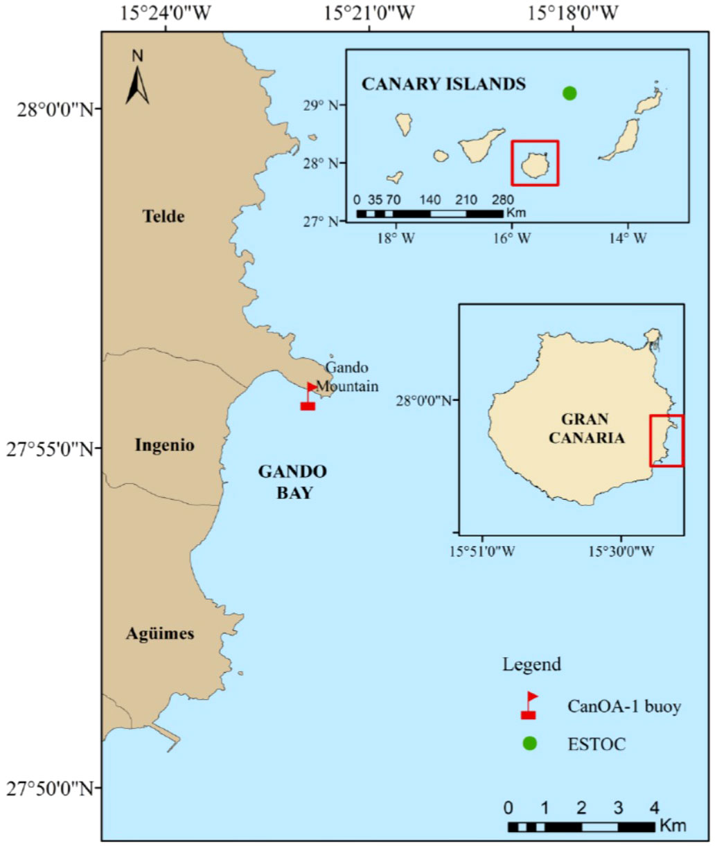
Figure 1 Study area map. The Gando Bay belongs to Gran Canaria Island. Red flag represents the location of buoy and green point, the ESTOC station.

2.2 Data collection

The CanOA-1 buoy structure is equipped with an array of seven sensors, including sea surface temperature and salinity (SST and SSS respectively; SBE 37-SI/SIP Thermosalinometer MicroCAT sensor manufactured by Sea-Bird Scientific –accuracy for SST is ±0.002°C and for SSS is ±0.01 units), fluorescence (Cyclops-7F from Turner Designs with a detection limit of 0.03 µg L^-1), dissolved oxygen concentration (Optode 4835 Oxymeter, manufactured by Aanderaa with an accuracy<0.1 µmol L^-1), photometric pH (SAMI-pH meter from Sunburst, precision<0.003 ppm and accuracy ±0.01 units), pCO₂ (partial pressure of CO₂, here expressed as fugacity of CO₂ – fCO₂; measured with a CO₂-pro CV sensor from PrOceanus - precision ±0.01 ppm and accuracy ±0.5%, using a Non-Dispersive Infrared Detector - NDIR) operating on a three-hour schedule, measuring the molar fraction of CO₂ (xCO₂) and converted internally to pCO₂ in seawater using a CO₂-permeable membrane. An external Sea-Bird Scientific pump (SBE-5) supplies seawater from outside the buoy body (60 cm), including copper-intake tubing to reduce biofouling effects. An internal zero determination is made every 24 hours to eliminate any signal drift. The pCO₂ was also measured using a Battelle system (model 635108H1010), which assesses the xCO₂ in both seawater and the atmosphere every three hours using equilibration-CO₂ Infrared detection. Atmospheric xCO₂ data from the Battelle system at 2.5 m above sea level, were calculated to 10 m (Hsu et al., 1994) and compared with those obtained at the ICOS Izaña Atmospheric Research Station (Tenerife, Canary Islands) and provided by the Agencia Estatal de Meteorología (AEMET). The agreement was better than ± 3 ppm. After the first year of work, the Batelle system had to be repaired so the Izaña data was used. Various meteorological variables (wind speed, wind direction, air temperature, humidity, atmospheric pressure, precipitation, solar radiation, and GPS coordinates – Gill MaxiMet GMX 501 GPS) were measured. All the sensors were installed at a depth of 1.5 m depth except for the meteorological station that was located 2.5 m above sea level. All data are free and the last 2000 data are available in real-time on the free Telegram app under Boya Morgan (@QUIMAbot).

Despite all the sensors installed on the buoy, the pH, chlorophyll and oxygen data have not been used due to their low stability and biofouling problems. In this sense, the pH sensor showed high variability and the pH data used in the manuscript were computed from total alkalinity to salinity relationship.

The buoy was visited every 2-3 months for inspection and maintenance. In addition, to determine the sensitivity and accuracy of the sensors, 23 surface water samples (with duplicates) were collected throughout the observation period. These samples were analyzed in the laboratory for total alkalinity (A_T), total dissolved inorganic carbon (C_T), and oxygen concentration. A_T and C_T were determined using the VINDTA 3C system (Mintrop et al., 2000) with Certified Reference Material (CRM) from batches 108, 122, 163, 177 and 196, provided by A. Dickson (Scripps Institute of Oceanography, University of South California, San Diego, United States) with allowed accuracy of ±1.5 μmol kg^-1 for both C_T and A_T. Oxygen was measured using the Winkler method (Granéli and Granéli, 1991). These laboratory measurements were subsequently used to verify the response of the various sensors (see below) and to establish relationships with continuous salinity data. Additionally, each measurement of CO₂ obtained by the Battelle sensor was calibrated every 3-hours prior to analysis using a zero and an external CO₂ gas cylinder with a known concentration of 553.35 ± 0.02 ppm traceable to the World Meteorological Organization.

2.3 Data treatment

The Battelle sensor provides xCO₂ values while the PrOceanus sensors provide pCO₂. The xCO₂ data were converted to pCO₂ (pCO_2,equ; Dickson et al., 2007) (Equation 1). The pCO_2,equ is the partial pressure of CO₂ in the equilibrator, P_atm (atm) is the atmospheric pressure and the expression for water vapor (pH₂O) is given in Equation 2. SST (K) is the sea surface temperature and SSS is the measured salinity. Once pCO₂ was obtained, the fCO₂ was calculated (Equation 3). The coefficients $B_{CO2}$ (cm³ mol^-1) and ${\delta }_{CO2}$ are given by Equations 4 and 5, respectively.

$\begin{array}{ll}pC{O}_{2,equ}=xC{O}_2\times (P_{atm}-p{H}_{2}O)& (1)\end{array}$

$\begin{array}{ll}p{H}_{2}O=e^{24.4543-67.4509\times \frac{100}{SST (K)}}-4.8489\times \ln \left(\frac{SST}{100}\right)-5.4\times {10}^{-4}\times SSS& (2)\end{array}$

$\begin{array}{ll}fC{O}_2=pC{O}_2\times EXP\lceil \frac{(B_{CO2}+2\times {((1-xC{O}_2))}^2\times {\delta }_{CO2})\times P_{equ}}{R\times SST}\rceil & (3)\end{array}$

$\begin{array}{ll}{B}_{CO2}=-1636.75+12.0408\times SST(K)-{3.2795710}^{-2}\times SS{T}^2(K)+{3.1652810}^{-5}\times SS{T}^3(K) & (4)\end{array}$

$\begin{array}{ll}{\delta }_{CO2}=57.7-0.118\times SST(K) & (5)\end{array}$

To determine the CO₂ flux (FCO₂) between the atmosphere and the sea surface water, Equations 6 and 7 were used:

$\begin{array}{ll}FC{O}_2=0.24\times S\times k\times \mathrm{\Delta }fC{O}_2 & (6)\end{array}$

$\begin{array}{ll}k=0.251\times w^2\times {\left(\frac{Sc}{600}\right)}^{-0.5} & (7)\end{array}$

where 0.24 is a conversion factor to have the flux in mmol m^-2 d^-1, S is the CO₂ solubility in mol dm^-3 atm^-1 (Weiss, 1970), and ΔfCO₂ is the difference between fCO₂ in seawater and atmosphere (fCO_{2 SW}-fCO_{2 atm}). k is the gas transfer velocity given by Wanninkhof (2014), where w is the wind velocity in m s^-1 (at 10 m height), Sc is the Schmidt number which considers the kinematic viscosity of seawater divided by the gas diffusion coefficient (Wanninkhof, 2014). The FCO₂ flux depends on the difference between fCO₂ in the seawater and the atmosphere, the temperature, and the wind speed. If the flux is negative, the ocean acts as a sink, and if it is positive, it acts as a source. Wind speeds were averaged from two hours before and two hours after each study point.

The fCO_2Tmean was calculated at the approximate annual mean temperature (21°C) (Takahashi, 1993) to obtain the temperature-independent fCO₂ (Equation 8). Hence, the annual non-thermal effect is obtained by the difference of the minimum and the maximum values obtained in Equation 9. The same process was followed to know the thermal effect (Equation 10) on the average observed fCO₂. The annual thermal effect was determined by the difference of the minimum and maximum values (Equation 11).

$\begin{array}{ll}fC{O}_{2Tmean}=fC{O}_{2Tobs}\times e^{[0.0423(T_{mean}-T_{obs})]} & (8)\end{array}$

$\begin{array}{ll}\mathrm{\Delta }{(fC{O}_2)}_{non-therm}={[fC{O}_{2Tmean}]}_{max}- {[fC{O}_{2Tmean}]}_{min} & (9)\end{array}$

$\begin{array}{ll}fC{O}_{2Tobs}=fC{O}_{2Tmean}\times e^{[0.0423(T_{obs}-T_{mean})]} & (10)\end{array}$

$\begin{array}{ll}\mathrm{\Delta }{(fC{O}_2)}_{therm}={[fC{O}_{2Tobs}]}_{max}- {[fC{O}_{2Tobs}]}_{min} & (11)\end{array}$

The thermal to non-thermal ratio (T/NT) shows the importance of both (physical and biological) effects. It was calculated by dividing the terms in Equations 9 and 11 ($\mathrm{\Delta }{(fC{O}_2)}_{therm}/\mathrm{\Delta }{(fC{O}_2)}_{non-therm}$ indicating that when the ratio is greater than 1, the temperature effect dominates over the other effects.

Total dissolved inorganic carbon (C_T), pH at in situ temperature (pH_T,IS) and normalized to a mean temperature of 21°C (pH_{T, T=21°C}) were calculated with the Excel program CO₂sys (Pierrot et al., 2021) using total alkalinity (computed from salinity) and the measured pCO₂ in seawater. The carbonic acid dissociation constants of Lueker et al. (2000), the HSO₄^- dissociation constant of Dickson (1990) and the value of [B]_I determined by Lee et al. (2010) were used.

Alkalinity concentrations used in the calculations (data not shown) were obtained from in situ samples (n=23, collected every 2-3 months) and normalized to a salinity (SSS) of 35 (NA_T = A_T/SSS·35). A constant value for NA_T = 2292.3 ± 2.8 μmol kg^-1 was obtained (similar to that obtained at the ESTOC site, located 60 miles north of the buoy site, González-Dávila et al., 2010), confirming that alkalinity is controlled by salinity variability and is not affected by atmospheric CO₂ increase or spring-summer primary productivity. In addition, since the SAMI sensor failed due to bubbles in the tubing, the pH was calculated in the total scale (pH_T) with alkalinity determined from salinity and pCO₂ variables.

The A_T-C_T pair of discrete data were used to test pCO₂ sensor values (23 pairs) and other carbonate system variables. The computed pCO₂ values and those provided by the sensor for the same day and time of the day were within ± 6 μatm. Calculated pH_T values from the A_T-C_T discrete values pair and those from A_T from salinity and sensor pCO₂ data were within ± 0.01 pH units. Moreover, discrete C_T concentrations (n = 23) and those determined from A_T from salinity and sensor pCO₂ data were within ± 3 μmol kg^-1.

The surface water displacement was calculated using the Ekman Equations 12 and 13, which include variables such as DE (Ekman depth), z (depth of interest, in this case, 8 meters), f (Coriolis parameter), and Az (turbulent viscosity coefficient). The solution to this equation yields a displacement angle of 45° when z is 0, meaning that the surface current flows at an angle of 45° to the right of the wind direction (Pond and Pickard, 1983). This calculated value was then added to the measured wind direction for further analysis.

$\begin{array}{ll}t=\left(\frac{\pi }{4}+\frac{\pi }{D_E}\right)exp\left(\frac{\pi }{D_E}\times z\right) & (12)\end{array}$

$\begin{array}{ll}{D}_{E=}\pi {\left(\frac{2A_z}{\left|f\right|}\right)}^{\frac{1}{2}} & (13)\end{array}$

2.4 Seasonal detrending of data

The trend analysis performed on the observed data includes inherent seasonal variability, which is influenced by sampling irregularities throughout the study period. To mitigate this seasonality, a seasonal detrending approach was implemented, in line with methodologies used in other time series analyses (e.g., Bates, 2012; González-Dávila and Santana-Casiano, 2023). The data were organized into corresponding monthly bins, spanning the time series from 2020 to 2023. Within each month, the mean and standard deviation were computed. Anomalies were then determined by subtracting the monthly mean from each data point within the dataset. This procedure effectively mitigated the temporal non-uniformity present in the data. Furthermore, a harmonic fitting technique was applied, similar to methods previously used in studies such as those conducted at the ESTOC site (González-Dávila et al., 2010). This fitting allows the determination, in a single step, of both seasonal effects (terms c, d, e, f) and interannual trends (b, Equation 14) as a function of time for the variable considered (y), expressed as an annual fraction (x). The results of this harmonic fitting analysis gave trends that closely aligned with those obtained within the estimated error margins for each considered parameter.

$\begin{array}{ll}\text{y}=\text{a}+\text{b }(\text{x}-2020)+\text{c sin }(2\pi \text{ x})+\text{d cos }(2\pi \text{ x})+\text{e sin }(4\pi \text{ x})+\text{f cos }(4\pi \text{ x})& (14)\end{array}$

3 Results

3.1 Hydrographic variability

The study area is characterized by a seasonal amplitude of SST as depicted in Figure 2A, with a range of approximately 5-6°C, fluctuating between 19°C and 24.8°C. The lowest SST were recorded in March, ranging from 18.8 - 19.3°C, while the highest SST were observed in September-October, ranging from 24.5 - 24.8°C. It is noteworthy that the minimum SST was registered in the year 2022, with SST reaching 18.8°C. During the period from 2020 to 2023, the average SST was 21.2 ± 1.6°C. Even if three years of data are not enough to obtain a significant trend analysis, it is observed that the surface waters in the study area exhibit a warming trend at a rate of 0.007°C yr^-1 (Table 1; SupplementaryFigure SI-1), a value that is consistent with solid trends shown by 25 years of ESTOC data (i.e. González-Dávila and Santana-Casiano, 2023). It is worth noting that there is a seasonal shift in SST, with the warmest temperatures typically occurring in July and August, comparable to the usually warmer months of September and October (Curbelo-Hernández et al., 2021; González-Dávila and Santana-Casiano, 2023), indicating that factors other than warming are acting on these coastal waters.

Figure 2

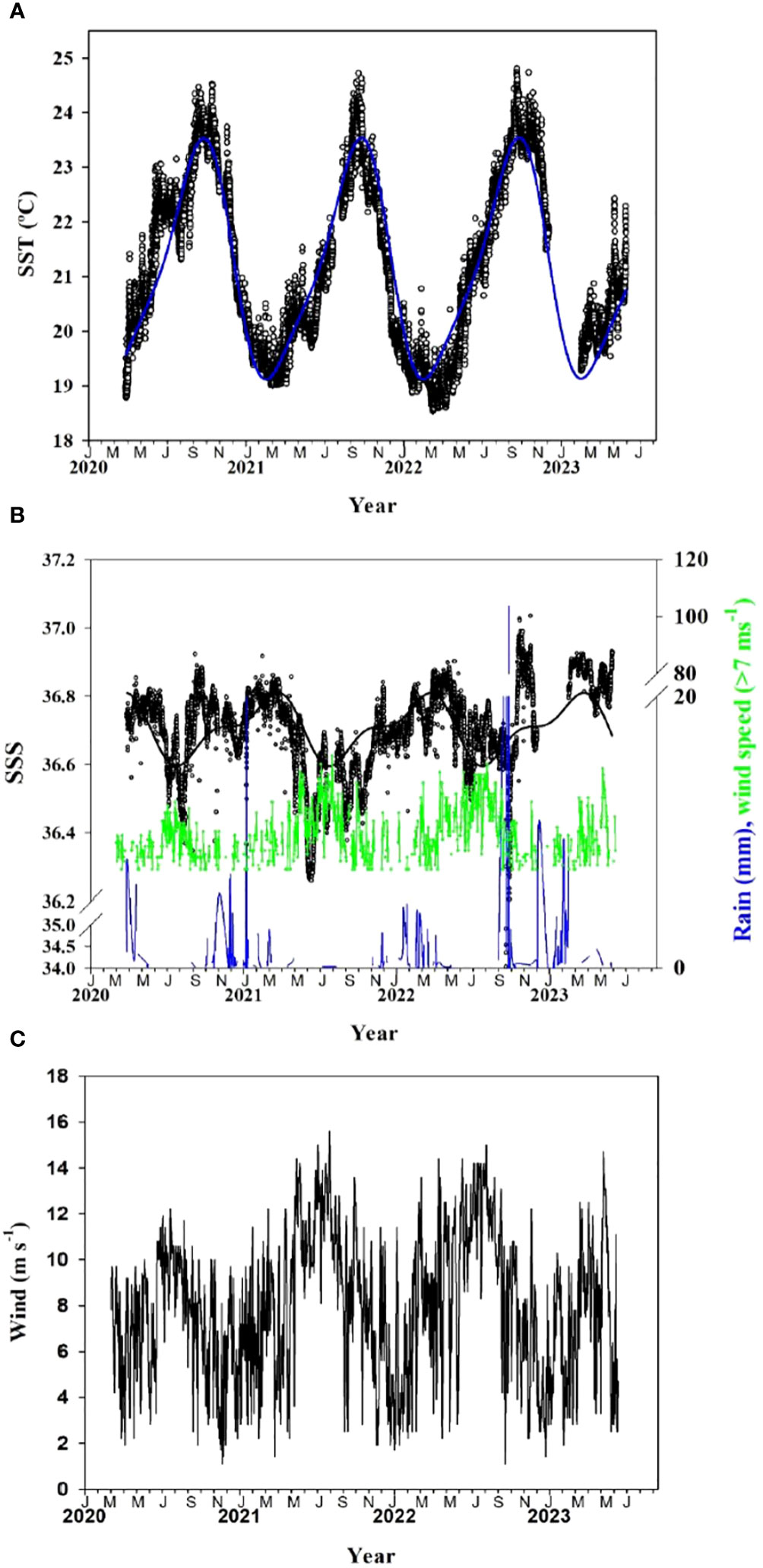
Figure 2 Sea Surface Temperature (SST, °C) (A), Sea Surface Salinity, rain (mm) and wind speed (m s^-1) for the stronger winds > 7 m s^-1 (B), and all the wind data [(C), m s^-1] recorded at the CanOA-1 site. The lines in (A) and (B) correspond to the harmonic fit of the observed data.

Table 1

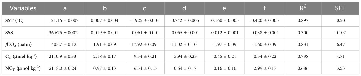
Table 1 Variables for the equations of interannual trend of the different variables monitored in the Gando Bay, according with Equation 14 where x is the year fraction of each observation y.

The SSS exhibited distinct characteristics during the 2020-2023 period (Figure 2B). The SSS reached its maximum salinities, ranging from 36.92 to 37.04, during the months of September and October. At certain time points, the SSS dropped to as low as 34 (e.g., SSS = 34.02 in September 2022), coinciding with periods of heavy rainfall (Figure 2B). The mean SSS observed throughout the study period was 36.71 ± 0.14. It was also observed that coinciding with the dominance of the Trade Winds from May to September (Figure 2B, green data, and Figure 2C), when the wind speed was above 7 m s^-1, low anomalous salinities were registered with respect to those described by the harmonic fit. The salinity has increased by 0.02 ± 0.001 during the observed period (Table 1; Figure 2B; Supplementary Figure SI-1).

3.2 Seasonality of the carbon system

Figure 3A shows that both CO₂ sensors provided highly consistent data (linear relationship with r² = 0.962, where the root mean square deviation (RMSD) was 2.9 µatm, n = 4600). The temporal overview of the fCO₂ in both the atmosphere and surface water within the study area is shown in Figure 3A. The average atmospheric fCO_2,atm was 415 ± 4 µatm. Surface water fCO_2sw showed variability, with the highest values occurring in September and October, reaching a maximum of 444 µatm (in September 2021). Conversely, the lowest fCO_2sw values were observed during the coldest months, particularly in February and March, when they hovered around 368 µatm. Consequently, a more pronounced seasonal fCO_2sw amplitude of about 55 - 60 µatm, was observed in the surface water compared to the atmosphere (about 12 µatm). Remarkably, in March 2023, the fCO_2sw values did not reach the lowest values observed in previous years, only decreasing to 384 µatm. This trend suggests that the surface water is undersaturated with CO₂ relative to the atmosphere in cold months, whereas it becomes oversaturated in warm months. As mentioned above, three years of data provide only a first estimate of any trend, including the fact that more local events are acting on coastal areas than in open ocean waters making more complex the calculation of a definitive trend. Nevertheless, the fCO_2sw values for the period 2020-2023 increase with an annual rate of 1.9 ± 0.1 µatm yr^-1 (Table 1) in the study area, considering both the harmonic fitting (Equation 14; Figure 3A; Table 1) and the detrended calculation (Supplementary Figure SI-1). This value is similar to that observed at the ESTOC site (González-Dávila and Santana-Casiano, 2023), which supports the values observed during these three years in Gando Bay.

Figure 3

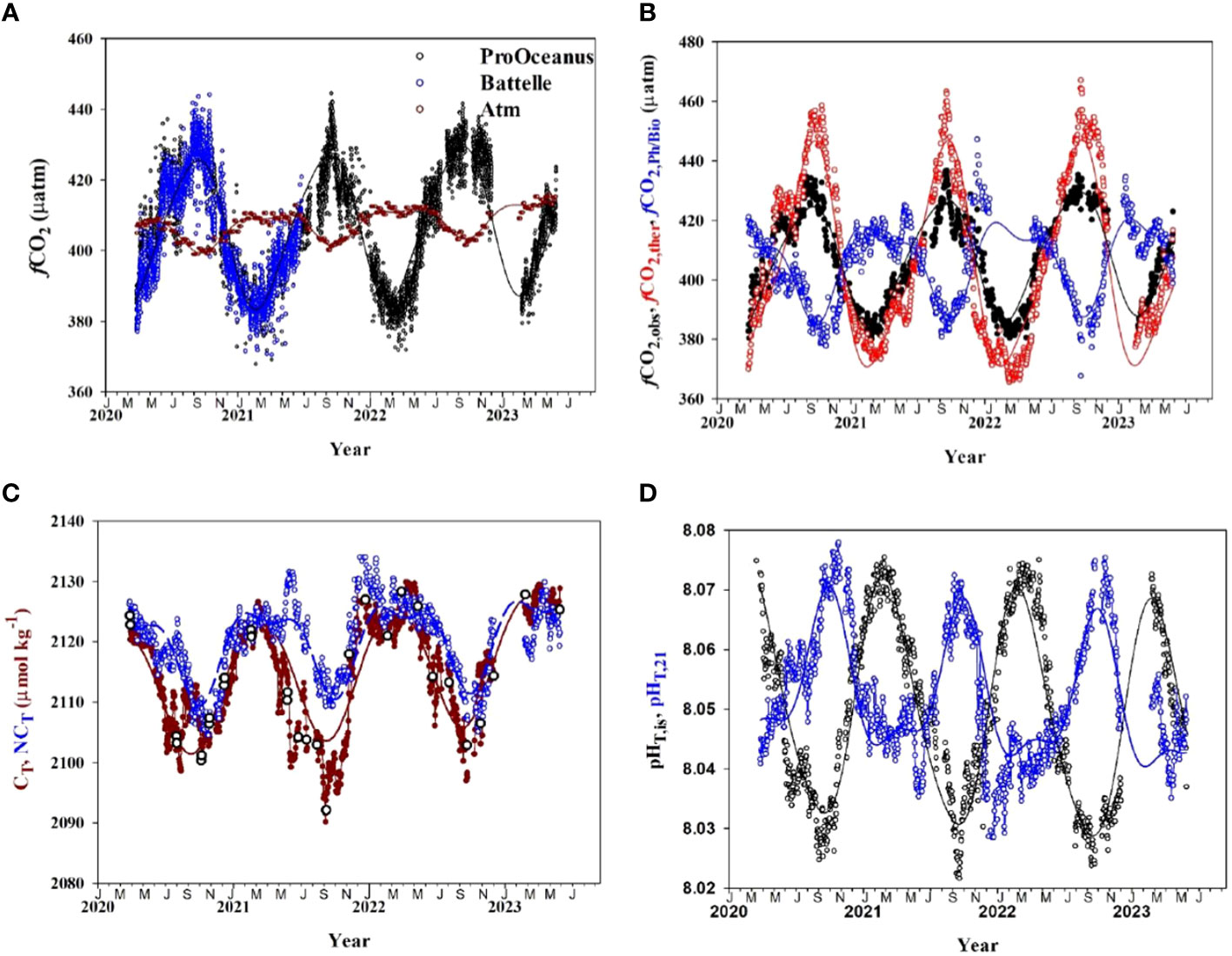
Figure 3 Evolution of fCO₂ in the atmosphere and ocean (A), the components of the fCO_2sw, considering the thermal (fCO_2,therm) and non-thermal processes (fCO_{2,non−therm}) (B), the total inorganic carbon (C_T) (estimated in red and measured in black) and seawater salinity-normalized inorganic carbon (NC_T) at SSS= 36.8 (C), and the pH at total scale, both at in situ temperature (pH_T,IS) and at constant temperature of 21°C (pH_T,21) (D), in the CanOA-1 site. The lines correspond to the harmonic fit of the data.

Figure 3B shows the decomposition of fCO_2sw together with the observed values (black dots) to assess the influence of thermal and non-thermal processes. In this study area, SST appears to control fCO_2sw, although the contributions of other physical mixing processes and biological factors should not be overlooked.

Figure 3C shows C_T measured with discrete samples and the C_T estimated from fCO₂ and A_T derived from SSS, in the study area. Concentrations decreased from colder to warmer months, with an average concentration of 2113 ± 8 μmol kg^-1 (Figure 3C). Maximum C_T typically occurred from mid-March to April, averaging 2123 ± 7 μmol kg^-1. Minimum concentrations were observed at the end of October, with an average of 2101 ± 3 μmol kg^-1. These observations suggest a seasonal amplitude of about 20 μmol kg^-1. During the observation period, C_T showed an increase of 2.2 ± 0.2 μmol kg^-1 yr^-1 (Table 1). However, when the C_T data were normalized to a constant salinity of 36.8 (NC_T = C_T/SSS·36.8) (Figure 3C), which removes precipitation and evaporation effects, the rate of increase was reduced to 1.0 ± 0.1 μmol kg^-1 yr^-1, a value similar to the oceanic ESTOC site (González-Dávila and Santana-Casiano, 2023).

The computed pH measurements, both in situ (pH_T,IS) and calculated at a constant temperature of 21°C (pH_T,21), are shown in Figure 3D. The pH_T,IS displayed a decreasing trend from winter to summer, with a mean value of 8.05 ± 0.02, for the studied period. The maximum pH_T,IS was typically recorded between February and March, with a mean of 8.07 ± 0.01, while minimum pH_T,IS occurred between September and October, averaging 8.03 ± 0.01. This variation represents a decrease of about 0.04 units from winter to summer. Characterizing a rate of change in a variable such as pH will need an extended time series of data. However, when detrended pH data at ESTOC site (period 1995-2023, Gonzalez-Dávila and Santana-Casiano, 2023) and those at the CanOA-1 site are plotted together (Figure 4), it is shown the coastal pH values are following the same pH trend than that at oceanic waters, this last one decreasing at 0.002 ± 0.0002 units yr^-1 (Figure 4; Supplementary Figure SI-1). It is also consistent with other oceanic carbon time series (Bates et al., 2014).

Figure 4

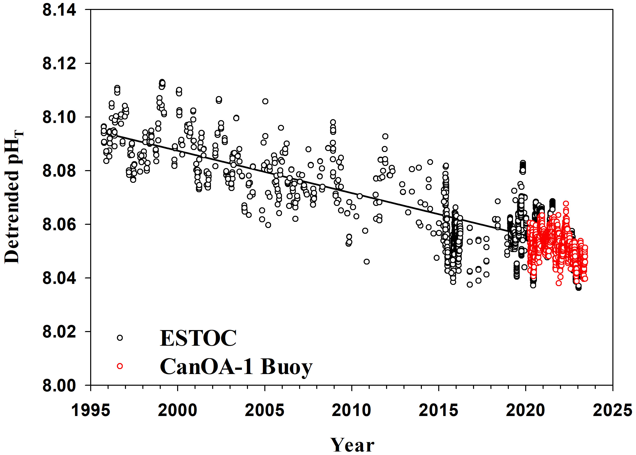
Figure 4 Detrended pH data in total scale measured at ESTOC (in black, González-Dávila and Santana-Casiano, 2023) and CanOA sites (in red).

Examination of the variability of fCO_2sw and the corresponding CO₂ flux (Figure 5) revealed periods of oversaturation (higher levels of fCO_2sw than those in fCO_2atm) from May and June to November and December, approximately. During these months, the coastal zone acted as a source of CO₂, releasing it from the ocean into the atmosphere. Conversely, during the rest of the year, the coastal zone acted as a carbon sink. It is noteworthy that on average ΔfCO₂ is lower during the period June to November than during the period December to June (Figure 3A). However, the highest FCO₂ coincided with the June to November period, indicating the effect of the increased wind intensity. In this region, the prevailing Trade Winds exhibit their maximum strength in July and August, with wind speeds reaching 16 m s^-1 (Figure 2C). During this period, it is common for wind speeds to consistently exceed 7 m s^-1 each year (Santana-Casiano et al., 2007).

Figure 5

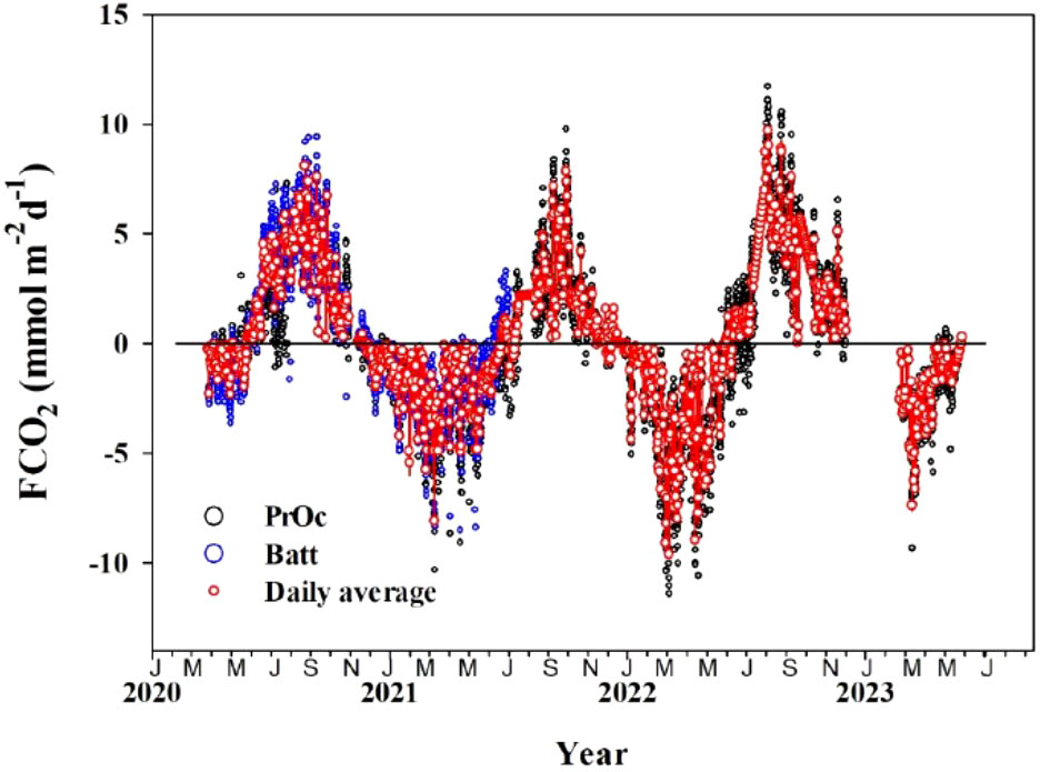
Figure 5 CO₂ flux (FCO₂) in the CanOA-1 site measured with two sensors as described in the experimental section. PrOc referred to the ProOceanus sensor and Batt is to the Battle sensor.

The mean annual flux of FCO₂ showed different patterns in the studied years when considered from March to March, with values of 0.70 ± 0.03 mmol m^-2 d^-1 (2020), -0.22 ± 0.04 mmol m^-2 d^-1 (in 2021), and 0.55 ± 0.04 mmol m^-2 d^-1 (in 2022). The average flux from 2020 to 2023 was 0.34 ± 0.04 mmol m^-2 d^-1 (126 ± 13 mmol m^-2 yr^-1), acting as a slight CO₂ source. The years 2020 and 2022 were registered as CO₂ sources with 255 mmol m^-2 yr^-1 and 202 mmol m^-2 yr^-1, respectively. Year 2021 acted as a slight sink of 79 mmol m^-2 yr^-1, related to lower SST in the area during winter months (Figure 2A). When extrapolated to the entire 6 km² area of Gando Bay (Figure 1), the region acted as a slight CO₂ source for the entire 2020-2022 period, quantified at 33 ± 3 tons of CO₂ yr^-1.

4 Discussion

Long-term time series data of CO₂ variables in coastal ecosystems are a rare but essential resource for assessing their response to climate change. In particular, time-series data that include at least two carbonate system variables are essential for understanding the underlying processes governing observed trends. In regions close to the coastline, such as the studied area, which has a depth of approximately 10 meters, variables such as wind intensity and direction, SST, and primary production exert certain influence.

In the context of this specific study, it is evident that forcing factors such as strong winds and precipitation events, such as tropical storms Theta (November 2020), Filomena (January 2021), and Hermine (September 2022), have a discernible impact on sea surface salinity (SSS, Figure 2B). Wu et al. (2021) previously demonstrated the influence of extreme events, such as typhoons, on the net atmosphere-ocean CO₂ exchange in the East China Sea, due to the water mixing and biological drawdown. In addition, the increase in SST, and also the atmospheric temperature due to extreme events such as heat waves occurring in the Canary Islands (Suárez-Molina and Sanz, 2022) also affects the CO₂ system through the dependence of fCO₂ on SST. In this sense, the Canary Islands have experienced several heat waves (AEMET, 2023): three in 2021 (11 days, 5 in August and 3 + 3 in September), two in 2022 (3 + 3 in July) and 26 days in 2023 (5 + 5 days in August and 16 days in October).

The study area, a coastal region with a natural barrier in the form of Mountain Gando (Figure 1), approximately 100 meters in height (IDE Canarias - https://visor.grafcan.es/), experiences fluctuations in wind intensity and direction, particularly within a few meters (approximately 50 meters) above the surface. These wind-related variations influence the water circulation patterns within the Gando Bay, resulting in lower SSS (Figure 2B) during periods of strong winds or winds blowing from certain directions. In this regard, a comprehensive analysis of the prevailing winds in the region and the surface water direction (Supplementary Figure SI-2) shows maximum wind speeds of 15 m s^-1 and an average of 8.2 ± 2.1 m s^-1 throughout the study period. The Trade Winds, which blow from the northeast direction (Van Camp et al., 1991), shift to the north-northwest in the study area due to the sheltering effect of the prominent Gando Mountain, forming a small peninsula that changes the wind direction (Supplementary Figure SI-2). These prevailing winds lead to a surface water column displacement of up to 8 meters in the W-SW direction at times. The calculation of this surface water displacement was achieved using the Ekman Equations (see experimental section).

Consistent findings, as established by Pond and Pickard (1983), confirm that surface currents in the Northern Hemisphere flow at an angle of 45° to the right of the prevailing wind direction. This displacement of surface water instigates the upward movement of deep water to compensate for the lost volume, a phenomenon elucidated by Kämpf and Chapman (2016). The replenishing seawater from deeper areas outside of the bay (about 150 m water depth), exhibits specific characteristics, with an average temperature of 22°C, a mean salinity of 36.4, a substantial C_T concentration of 2117 μmol kg^-1, and a mean pH_T,IS of 8.03 (Curbelo-Hernández et al., 2023). Notably, these values differ from the typical surface conditions in the bay during June-August, which include SST of 23.5°C, SSS reaching up to 36.7, C_T concentrations of 2105 μmol kg^-1, and a pH_T,IS of 8.04. In this sense, it was observed every year that there was no increase in SST from June to September, but the SST was relatively constant or even decreased by July-August consisting with the strongest predominant Trade winds blowing in the area that favored the entrance of deeper water from outside of the bay. Depending on the wind strength and the moment when that force is exerted, it is observed that the increase in SST does not consistently rise but rather slows down due to the arrival of colder water and increased surface mixing. During these periods of decreasing SST, an increase in SSS variability was observed, also related to the arrival of deeper water with lower salinity and pH and higher C_T (Figure 2B).

Efforts were made to discern any potential correlation with tidal intensity throughout the lunar period (SupplementaryFigure SI-3). Although some instances of alignment between full and new moon phases and variations in SSS were identified, these occurrences lacked temporal consistency. Consequently, while tidal effects may exert some influence, they do not appear to constitute a primary or determinative factor within this particular environment. Nonetheless, it is worth noting that tidal height plays a crucial role in carbon exchange within estuaries and river mouth regions, as highlighted in previous studies (Ortega et al., 2005; Bauer et al., 2013).

The hydrographic features of Gando Bay are manifested in the seasonal and interannual variability of the CO₂ variables. The interannual increase of fCO_2sw, quantified at 1.9 µatm yr^-1 (Table 1; Figures 3A, B), considering only three years of data is close to the observed value at the oceanic station ESTOC of 2.1 ± 0.1 µatm yr^-1 (González-Dávila and Santana-Casiano, 2023), indicating the important control of the increased atmospheric CO₂ concentrations in the seawater concentration. Further years of observation are required to confirm this trend in Gando Bay. During the year, thermodynamic effects control the observed variability (Figure 3B) with a T/NT ratio of 2.0 ± 0.1, but other physical and biological effects should not be ignored. From February to November (Figure 3B, black dots), the increase in SST led to an increase in measured fCO_2sw (a slope of 10 ± 0.2 μatm °C^-1 was calculated). According to Takahashi (1993), the theoretical change should be 17 μatm °C^-1 (indicated by the red dots in Figure 3B). The observed lower slope in Gando Bay includes both the effects of the arrival of deeper, less saline water with highly variable fCO_2sw content and changes in the productivity of the area (blue dots in Figure 3B). Oxygen data from the sensor (data not shown) were strongly affected by biofouling during the early years of study until a flow system with a copper intake located far from the buoy body was included. However, there is not enough oxygen data to decompose the nonthermal component between biological and water mixing processes. Moreover, there is a seagrass bed (locally known as sebadales) in the vicinity of the buoy which is known for its robust biological activity characteristics (Duarte and Krause-Jensen, 2017; Serrano et al., 2021). As mentioned above, the study area is impacted by the influence of the Trade Winds (wind direction and intensity), and the presence of the nearby mountain, all of which contribute to its unique characteristics, especially during the summer months period. The physical factors should also consider the influence of tides, wind, and horizontal mixing (Xue et al., 2016) on the impact of mixing processes between coastal and open ocean waters, mainly driven by horizontal advection, leading to changes in SSS and productivity, a phenomenon that should also affect the present study.

This outcome differs from the prevailing pattern in coastal regions, where changes in C_T due to non-thermal forcings are expected to dominate, especially in mid-latitudes (Cao et al., 2020; Torres et al., 2021). This unexpected result can be attributed to the shallow nature and low productivity of the coastal area studied (Arístegui et al., 2001), which differs from the conditions reported by these authors. Moreover, in the northern region of Gran Canaria (station 16.5°W), research by Curbelo-Hernández et al. (2021) revealed a T/NT ratio of 2.1, comparable to the results obtained in Gando Bay. Therefore, it can be inferred that in Gando Bay, despite the impact of non-thermal processes including encompassing biological activity and advective mixing, the thermal component controls the observed seasonality in the fCO_2sw. These climatological results parallel findings from other coastal studies, such as those conducted in Hawaii and Australian regions, where temperature dominantly controls fCO_2sw (Shaw and McNeil, 2014; Terlouw et al., 2019). In the northern coastal regions of the Atlantic Ocean, non-thermal processes control the fCO_2sw (Gac et al., 2020).

According to the observations, the decrease in pH_T,IS at the CanOA-1 site followed the same behavior as that at the oceanic ESTOC site, (Figure 4), and was comparable to other coastal areas such as SOMLIT-Brest, where pH decreased by -0.0026 ± 0.0004 yr^-1. The observed diurnal variation is linked with the diel biological cycle, such as in the Bay of Brest and the tidal cycles in Roscoff (Gac et al., 2020, 2021), and was of a similar magnitude to the seasonal variability. These results are consistent with previous studies of coastal seas in NW Europe that estimated ocean acidification based on seasonal cruises or voluntary observing ship surveys (Clargo et al., 2015; Ostle et al., 2016; Omar et al., 2019). Ocean acidification rates in North Sea surface waters ranged from -0.0022 yr^-1 (period 2001–2011; Clargo et al., 2015) to -0.0035 yr^-1 (period 1984–2014; Ostle et al., 2016), with a recent estimate of -0.0024 yr^-1 in the northern North Sea (Omar et al., 2019). When the temperature effect is eliminated, pH_T,21 shows an average of 8.05 ± 0.02 and follows an inverse pattern compared to pH_T,IS. pH_T,21 increases from February to September (mean of 8.07 ± 0.01) related to the increase of biological activity and decreases from September to February (mean of 8.03 ± 0.01) due to vertical mixing with deeper seawater from out of the bay and possible with higher nutrient concentrations. Unfortunately, we did not measure the biological activity, the nutrient concentration in the buoy location and oxygen data are not enough accurate to estimate this component. Despite its status as a coastal zone, the biodiversity in the area appears to be insufficient to absorb excess atmospheric CO₂ due to the results of T/NT ratio. Consequently, this leads to acidification levels in the region that are similar to those observed at the ESTOC oceanic station in the Northeast Atlantic, characterized by an interannual variability of -0.002 pH units yr^-1 (Santana-Casiano et al., 2007; González-Dávila et al., 2010; González-Dávila and Santana-Casiano, 2023).

The recorded C_T with an average of 2113 ± 8 μmol kg^-1 (for the study period) were close to the observed concentrations at the ESTOC station for the years 1995-2020 with an average of 2109.5 ± 9.6 μmol kg^-1. These concentrations converge if the observed annual C_T increase at ESTOC of 1.09 ± 0.10 μmol kg^-1 yr^-1 is applied (Bates et al., 2014). However, the observed trend of increase in C_T over the three-year period studied (2.2 ± 0.4 μmol kg^-1 yr^-1) is twice that observed in open oceanic waters at ESTOC. When the NC_T data are considered (Figure 3C, blue open circles), the trend is reduced to 1 ± 0.1, as that observed in ESTOC. Therefore, we assume that most of the anomalies with respect to the harmonic function are related to the arrival of deeper waters into the area, which could bring more remineralized (positive anomalies) or more productive (negative anomalies) waters. As a result, the NC_T does not decrease after the end of March, but keeps relatively constant concentrations until July, when the productivity of the area compensates the physical processes. The detectable seasonal amplitude of 15 μmol kg^-1 in NC_T after July (Figure 3C) is associated with CO₂ consumption by organisms for the production of organic matter and the exchange of CO₂ between the atmosphere and the surface layer. In this coastal area, the influence of the Trade Winds seems to be more important due to horizontal advection and seawater renewal in the bay.

The variability of fCO₂ in both the atmosphere and seawater describes the studied system as an overall CO₂ source. The surface water was undersaturated from late October to mid-June. For the rest of the year, the surface water was supersaturated and the system acted as a source. The calculated mean FCO₂ over the study period is 0.35 ± 0.04 mmol m^-2 d^-1 (126 ± 13 mmol m^-2 yr^-1), with peak outgassing occurring between August and November, and maximum ingassing observed between February and March. This shift from a sink to a source role coincides temporally with the onset of Trade Winds, which typically blow at high and constant velocity in the Canary Islands from mid-June. This climatology is consistent with previous coastal studies, such as those conducted in the Hawaiian region, where the influence of Trade Winds is prominent and affects the CO₂ system in coastal waters (Terlouw et al., 2019). The occurrence and strength of the dominant northeast and east Trade Winds between 1973 and 2009 have been previously studied (Garza et al., 2012) and reported velocities ranging from 0.8 to 8.2 m s^-1, with summer being the period of higher intensity. Furthermore, the significance of winds and mixing processes becomes clear when comparing these results with coastal studies along the East Australian coast, where mixing processes are relatively low (McNeil, 2010; Shaw and McNeil, 2014), or along the Northwest coast of the North Atlantic Ocean, where coastal systems act as CO₂ sinks primarily due to SST effects at higher latitudes (Boehme et al., 1998).

The FCO₂ results here are comparable to other coastal stations such as in Brest (France, Gac et al., 2020) and Hawaii (Terlouw et al., 2019). In Brest, at higher latitudes than the Canary Islands, the authors estimated fluxes of 0.18 ± 0.10, 0.11 ± 0.12, and 0.39 ± 0.08 mol m^–2 yr^–1 in three coastal stations. In Hawaii, it is also important to highlight how the coastal areas could be a strong source of CO₂ from the ocean with 1.24 ± 0.33 mol m⁻² yr⁻¹, and close to the equilibrium with 0.05 ± 0.02 and 0.00 ± 0.03 mol m⁻² yr⁻¹ at the other two coastal stations. In the coastal waters of the Mediterranean Sea, the coastal waters of the Gulf of Trieste act as a CO₂ sink in winter, especially in the presence of strong wind events (FCO₂ up to −11.9 mmol m⁻² d⁻¹; Cantoni et al., 2012; Ingrosso et al., 2016). In the Gando Bay region, with a net annual outgassing flux of 0.26 mol m^-2 yr^-1 (period 2020-2022), with values of 0.20 mol m^-2 yr^-1 for the years 2020 and 2022, but ingassing CO₂ at -0.08 mol m^-2 yr^-1 for the year 2021 due to lower winter SST values, the influence of Trade Winds is responsible for a temporary increase in fluxes, causing the mean values to remain positive (0.13 ± 0.01 mol m^-2 yr^-1), a phenomenon also observed at the ESTOC station (González-Dávila et al., 2003; Santana-Casiano et al., 2007; González-Dávila and Santana-Casiano, 2023). Additionally, Curbelo-Hernández et al. (2021) reported an average FCO₂ of -0.25 ± 0.04 mol m^-2 yr^-1 for the oceanic waters near Gran Canaria, which is consistent with the behavior observed in the Northeast Atlantic Ocean (-0.6 mol m^-2 yr^-1) (Takahashi et al., 2009).

Considering the mean flux determined at the coastal buoy site within Gando Bay (6 km²), a net annual outgassing flux of 33 ± 4 Tons of CO₂ per year through the bay is calculated, which is close to equilibrium. If we consider the values determined in the open ocean waters of the Canary Islands (Curbelo-Hernández et al., 2021), where a CO₂ sink of -0.24 ± 0.04 mol m^-2 yr^-1 was calculated, that is, -170 Tons of CO₂ yr^-1 for the entire coastal area of the Canary Islands. Coastal areas located in the easternmost part of the archipelago are affected by the arrival of Northwest African coastal waters (Curbelo-Hernández et al., 2021). The Gando Bay, with an area of only 6 km², causes the amount of CO₂ absorbed by the Canary region to decrease by 9%.

Coastal regions at lower latitudes typically act as sources of CO₂ to the atmosphere, while high latitudes tend to act as sinks (Chen, 2004; Cao et al., 2020). Notably, the boundary for this behavior typically occurs around 30°N (Cai et al., 2006), placing the study area in the transition zone between low and high latitudes. Consequently, it is consistent with the result that this coastal area of the Canary Islands acts as a source while it is almost in equilibrium. The flux depends on several factors such as SST, ΔfCO₂, and wind speed. This makes different mixing processes and biological activity in both the coastal and open ocean environments crucial influencers of the carbonate system parameters and controllers of the CO₂ air-sea exchange. In the case of this study area, it remains relatively unaffected by rivers, agriculture, or other anthropogenic activities that could disrupt the biological activity and the physical processes that control the carbonate system in the region.

The findings of this research clearly emphasize the need to explore additional coastal areas, since the hydrodynamic and CO₂ system-altering phenomena exhibit pronounced locality. Their effects vary from one area to another. In addition, studies should also extend the observations for at least 10 years to allow more accurate estimates of rates of change.

5 Conclusion

The coastal zones of islands require vigilant monitoring to accurately quantify the carbon balance and its consequences as an essential tool for effective governance. The economic well-being of these islands is significantly intertwined with the health of their coastal zones.

Within the Canary Islands, the CanOA-1 station, an integral part of the international GOA-ON network, is located in the eastern region of Gran Canaria, specifically in the Bay of Gando. Data from this station show a discernible seasonal pattern in the variables defining the CO₂ system. This study highlights the importance of physical processes, especially horizontal mixing, biological influences (hypothesis because no biological data are collected), and sea surface temperature, in facilitating the transfer of CO₂ from the atmosphere to the ocean.

The three-year data allow us to know that the sea surface temperature (SST) shows seasonal fluctuations, with the highest temperatures occurring in September-October and the lowest in March. The contributions of both thermal and non-thermal processes to the seasonal fCO₂ were investigated with vertical mixing, wind stress, and biological forcing as principal components. The T/NT ratio of 2.0 ± 0.1 implies that SST plays a controlling role in modulating fCO_2sw, although the influence of other factors should not be neglected. fCO_2sw increases at a rate of 1.91 µatm yr^-1, which is consistent with the observed increase in NC_T in these coastal waters. The CO₂ transfer from the atmosphere to the surface waters causes a decrease of pH_T,IS in the region. Furthermore, the concentration of total inorganic carbon (NC_T) showed an annual increase of 1.0 μmol kg^-1 yr^-1 in the surface waters of the bay. The occurrence of extreme events, such as tropical storms, and the most persistent Trade Winds direction, which are modified by the geological structure of the bay, affect the physico-chemical properties of the region, renewing the bay waters with deeper seawater, affecting SSS, pH, fCO₂, and C_T.

According to the data collected at the CanOA-1 site, the Gando Bay is almost in equilibrium, with a total CO₂ release from the ocean to the atmosphere between 2020 and 2023, of 33 ± 4 Tons of CO₂ yr^-1, with the year 2021 acting as a slight sink. Small changes in SST between years, together with variability related to the prevailing strength of the Trade Winds, which affect both water exchange and CO₂ fluxes, control the Gando Bay site. This underscores the critical importance of continuous monitoring and quantification of CO₂ concentrations in seawater, especially in coastal regions and on islands worldwide, in order to estimate the CO₂ contribution of coastal regions to the global ocean.

Data availability statement

The raw data supporting the conclusions of this article will be made available by the authors, without undue reservation.

Author contributions

AG: Data curation, Formal analysis, Funding acquisition, Investigation, Writing – original draft. AA-R: Formal analysis, Writing – review & editing. DG-S: Formal analysis, Investigation, Writing – review & editing. MG-D: Conceptualization, Formal analysis, Funding acquisition, Investigation, Writing – review & editing. JC: Formal analysis, Funding acquisition, Investigation, Writing – review & editing.

Funding

The author(s) declare that financial support was received for the research, authorship, and/or publication of this article. This study was supported by the Government of the Canary Islands the Loro Parque Foundation through the CanBIO project, CanOA subproject (2019-2023) and the CARBOCAN agreement (Consejería de Transición Ecológica, Lucha contra el Cambio Climático y Planificación Territorial, Gobierno de Canarias). Discrete sampling and maintenance were also supported by the FeRIA project (PID2021-123997NB-100), the Spanish Ministerio de Ciencia e Innovación.

Acknowledgments

Special thanks go to the Mando Aéreo de Canarias (MACAN), its officers and all the members of the Base Aérea de Gando, and to all the marine supporting members for providing support (personnel and boats), assistance and surveillance.

Conflict of interest

The authors declare that the research was conducted in the absence of any commercial or financial relationships that could be construed as a potential conflict of interest.

Publisher’s note

All claims expressed in this article are solely those of the authors and do not necessarily represent those of their affiliated organizations, or those of the publisher, the editors and the reviewers. Any product that may be evaluated in this article, or claim that may be made by its manufacturer, is not guaranteed or endorsed by the publisher.

Supplementary material

The Supplementary Material for this article can be found online at: https://www.frontiersin.org/articles/10.3389/fmars.2024.1337929/full#supplementary-material

References

AEMET (2023). “Olas de calor en España desde 1975,” in Área de Climatología y Aplicaciones Operativas. Spain: AEMET. Available at: https://www.aemet.es/es/conocermas/recursos_en_linea/publicaciones_y_estudios/estudios/detalles/olascalor.

Google Scholar

Arístegui J., Hernández-León S., Montero M. F., Gómez M. (2001). The seasonal planktonic cycle in coastal waters of the Canary Islands. Scientia Marina 65, 51–58. doi: 10.3989/scimar.2001.65s151

CrossRef Full Text | Google Scholar

Bates N. R. (2012). Multi-decadal uptake of carbon dioxide into subtropical mode water of the North Atlantic Ocean. Biogeosciences 9, 2649–2659. doi: 10.5194/bg-9-2649-2012

CrossRef Full Text | Google Scholar

Bates N. R., Astor Y. M., Church M. J., Currie K., Dore J. E., González-Dávila M., et al. (2014). A time-series view of changing surface ocean chemistry due to ocean uptake of anthropogenic CO₂ and ocean acidification. Oceanography 27, 126–141. doi: 10.5670/oceanog.2014.16

CrossRef Full Text | Google Scholar

Bates N. R., Johnson R. J. (2020). Acceleration of ocean warming, salinification, deoxygenation and acidification in the surface subtropical North Atlantic Ocean. Commun. Earth Environ. 1, 33. doi: 10.1038/s43247-020-00030-5

CrossRef Full Text | Google Scholar

Bauer J. E., Cai W. J., Raymond P. A., Bianchi T. S., Hopkinson C. S., Regnier P. A. G. (2013). The changing carbon cycle of the coastal ocean. Nature 504, 61–70. doi: 10.1038/nature12857

PubMed Abstract | CrossRef Full Text | Google Scholar

Boehme S. E., Sabine C. L., Reimers C. E. (1998). CO₂ fluxes from a coastal transect: A time-series approach. Mar. Chem. 63, 49–67. doi: 10.1016/S0304-4203(98)00050-4

CrossRef Full Text | Google Scholar

Borges A. V. (2005). Do we have enough pieces of the jigsaw to integrate CO₂ fluxes in the coastal ocean? Estuaries 28, 3–27. doi: 10.1007/BF02732750

CrossRef Full Text | Google Scholar

Borges A. V., Delille B., Frankignoulle M. (2005). Budgeting sinks and sources of CO₂ in the coastal ocean: Diversity of ecosystem counts. Geophys. Res. Lett. 32, 1–4. doi: 10.1029/2005GL023053

CrossRef Full Text | Google Scholar

Borges A. V., Frankignoulle M. (2002). Distribution of surface carbon dioxide and air-sea exchange in the upwelling system off the Galician coast. Global Biogeochem. Cycles 16, 13–11. doi: 10.1029/2000GB001385

CrossRef Full Text | Google Scholar

Borges A. V., Gypensb N. (2010). Carbonate chemistry in the coastal zone responds more strongly to eutrophication than ocean acidification. Limnol. Oceanogr. 55, 346–353. doi: 10.4319/lo.2010.55.1.0346

CrossRef Full Text | Google Scholar

Borges A. V., Schiettecatte L. S., Abril G., Delille B., Gazeau F. (2006). Carbon dioxide in European coastal waters. Estuarine Coast. Shelf Sci. 70, 375–387. doi: 10.1016/j.ecss.2006.05.046

CrossRef Full Text | Google Scholar

Bouillon S., Borges A. V., Castañeda-Moya E., Diele K., Dittmar T., Duke N. C., et al. (2008). Mangrove production and carbon sinks: a revision of global budget estimates. Global biogeochem. cycles 22, 1–12. doi: 10.1029/2007GB003052

CrossRef Full Text | Google Scholar

Cai W. J. (2011). Estuarine and coastal ocean carbon paradox: CO₂ sinks or sites of terrestrial carbon incineration? Annu. Rev. Mar. Sci. 3, 123–145. doi: 10.1146/annurev-marine-120709-142723

CrossRef Full Text | Google Scholar

Cai W. J., Dai M., Wang Y. (2006). Air-sea exchange of carbon dioxide in ocean margins: A province-based synthesis. Geophys. Res. Lett. 33, 1–4. doi: 10.1029/2006GL026219

CrossRef Full Text | Google Scholar

Cantoni C., Luchetta A., Celio M., Cozzi S., Raicich F., Catalano G. (2012). Carbonate system variability in the gulf of Trieste (north Adriatic sea). Estuarine Coast. Shelf Sci. 115, 51–62. doi: 10.1016/j.ecss.2012.07.006

CrossRef Full Text | Google Scholar

Cao Z., Yang W., Zhao Y., Guo X., Yin Z., Du C., et al. (2020). Diagnosis of CO₂ dynamics and fluxes in global coastal oceans. Natl. Sci. Rev. 7, 786–797. doi: 10.1093/nsr/nwz105

PubMed Abstract | CrossRef Full Text | Google Scholar

Carstensen J., Duarte C. M. (2019). Drivers of pH variability in coastal ecosystems. Environ. Sci. Technol. 53, 4020–4029. doi: 10.1021/acs.est.8b03655

PubMed Abstract | CrossRef Full Text | Google Scholar

Chen C. A. (2004). Exchanges of carbon in the coastal seas. Eds. Field C. B., Raupach M. R. SCOPE. Washington DC: Island Press, 62.

Google Scholar

Chen C. T. A., Borges A. V. (2009). Reconciling opposing views on carbon cycling in the coastal ocean: Continental shelves as sinks and near-shore ecosystems as sources of atmospheric CO₂. Deep Sea Res. Part II: Topical Stud. Oceanogr. 56, 578–590. doi: 10.1016/j.dsr2.2009.01.001

CrossRef Full Text | Google Scholar

Chen C. A., Huang T. H., Chen Y. C., Bai Y., He X., Kang Y. (2013). Air-sea exchanges of the coin the world’s coastal seas. Biogeosciences 10, 6509–6544. doi: 10.5194/bg-10-6509-2013

CrossRef Full Text | Google Scholar

Clargo N. M., Salt L. A., Thomas H., De Baar H. J. (2015). Rapid increase of observed DIC and pCO₂ in the surface waters of the North Sea in the 2001-2011 decade ascribed to climate change superimposed by biological processes. Mar. Chem. 177, 566–581. doi: 10.1016/j.marchem.2015.08.010

CrossRef Full Text | Google Scholar

Curbelo-Hernández D., González-Dávila M., González A. G., González-Santana D., Santana-Casiano J. M. (2021). CO₂ fluxes in the Northeast Atlantic Ocean based on measurements from a surface ocean observation platform. Sci. Total Environ. 775, 145804. doi: 10.1016/j.scitotenv.2021.145804

PubMed Abstract | CrossRef Full Text | Google Scholar

Curbelo-Hernández D., González-Dávila M., Santana-Casiano J. M. (2023). The carbonate system and air-sea CO2 fluxes in coastal and open-ocean waters of the Macaronesia. Front. Mar. Sci. 10, 1094250. doi: 10.3389/fmars.2023.1094250

CrossRef Full Text | Google Scholar

de Haas H., van Weering T. C., de Stigter H. (2002). Organic carbon in shelf seas: sinks or sources, processes and products. Continent. Shelf Res. 22, 691–717. doi: 10.1016/S0278-4343(01)00093-0

CrossRef Full Text | Google Scholar

Denman K. L., Brasseur G. P., Ciais P., Cox P. M. (2007) Couplings between changes in the climate system and biogeochemistry. Available online at: https://www.researchgate.net/publication/224942928.

Google Scholar

Dickson G. (1990). The standard potential of the reaction: AgCl_(s) + 1 2H_2(g) = Ag(s) + HCl_(aq), and the standard acidity constant of the ion HSO₄^- in synthetic seawater from 273.15 to 318.15 K. J. Chem. Thermodynam. 22, 113–127. doi: 10.1016/0021-9614(90)90074-Z

CrossRef Full Text | Google Scholar

Dickson A. G., Sabine C. L., Christian J. R., (eds) (2007). Guide to best practices for ocean CO₂ measurements. (Sidney, British Columbia: North Pacific Marine Science Organization), 191. (PICES Special Publication 3; IOCCP Report 8). doi: 10.25607/OBP-1342

CrossRef Full Text | Google Scholar

Doney S. C., Fabry V. J., Feely R. A., Kleypas J. A. (2009). Ocean acidification: The other CO₂ problem. Annu. Rev. Mar. Sci. 1, 169–192. doi: 10.1146/annurev.marine.010908.163834

CrossRef Full Text | Google Scholar

Duarte C. M., Krause-Jensen D. (2017). Export from seagrass meadows contributes to marine carbon sequestration. Front. Mar. Sci. 4. doi: 10.3389/fmars.2017.00013

CrossRef Full Text | Google Scholar

Falkowski P. G., Wilson C. (1992). Phytoplankton productivity in the North Pacific ocean since 1900 and implications for absorption of anthropogenic CO₂. Nature 358, 741–743. doi: 10.1038/358741a0

CrossRef Full Text | Google Scholar

Friedlingstein P., O’Sullivan M., Jones M. W., Andrew R. M., Gregor L., Hauck J., et al. (2022). Global carbon budget 2022. Earth Syst. Sci. Data 14, 4811–4900. doi: 10.5194/essd-14-4811-2022

CrossRef Full Text | Google Scholar

Friedlingstein P., O’Sullivan M., Jones M. W., Andrew R. M., Hauck J., Olsen A., et al. (2020). Global carbon budget 2020. Earth Sys. Sci. Data 12, 3269–3340. doi: 10.5194/essd-12-3269-2020

CrossRef Full Text | Google Scholar

Gac J. P., Marrec P., Cariou T., Grosstefan E., Macé É., Rimmelin-Maury P., et al. (2021). Decadal dynamics of the CO₂ system and associated ocean acidification in coastal ecosystems of the north east Atlantic Ocean. Front. Mar. Sci. 8. doi: 10.3389/fmars.2021.688008

CrossRef Full Text | Google Scholar

Gac J. P., Marrec P., Cariou T., Guillerm C., Macé É., Vernet M., et al. (2020). Cardinal buoys: an opportunity for the study of air-sea CO₂ fluxes in coastal ecosystems. Front. Mar. Sci. 7. doi: 10.3389/fmars.2020.00712

CrossRef Full Text | Google Scholar

Garza J. A., Chu P. S., Norton C. W., Schroeder T. A. (2012). Changes of the prevailing trade winds over the islands of Hawaii and the North Pacific. J. Geophys. Res.: Atmos. 117, 1–18. doi: 10.1029/2011JD016888

CrossRef Full Text | Google Scholar

Gattuso J. P., Frankignoulle M., Wollast R. (1998). Carbon and carbonate metabolism in coastal aquatic ecosystems. Annu. Rev. Ecol. System. 29, 405–434. doi: 10.1146/annurev.ecolsys.29.1.405

CrossRef Full Text | Google Scholar

González-Dávila M., Santana-Casiano J. M. (2023). Long-term trends of pH and inorganic carbon in the Eastern North Atlantic: the ESTOC site. Front. Mar. Sci. 10. doi: 10.3389/fmars.2023.1236214

CrossRef Full Text | Google Scholar

González-Dávila M., Santana-Casiano J. M., González-Dávila E. F. (2007). Interannual variability of the upper ocean carbon cycle in the northeast Atlantic Ocean. Geophys. Res. Lett. 34, 1–7. doi: 10.1029/2006GL028145

CrossRef Full Text | Google Scholar

González Dávila M., Santana-Casiano J. M., Merlivat L., Barbero-Muñoz L., Dafner E. V. (2005). Fluxes of CO₂ between the atmosphere and the ocean during the POMME project in the northeast Atlantic Ocean during 2001. J. Geophys. Res. C: Oceans 110, 1–14. doi: 10.1029/2004JC002763

CrossRef Full Text | Google Scholar

González-Dávila M., Santana-Casiano J. M., Rueda M. J., Llinás O. (2010). The water column distribution of carbonate system variables at the ESTOC site from 1995 to 2004. Biogeosciences 7, 3067–3081. doi: 10.5194/bg-7-3067-2010

CrossRef Full Text | Google Scholar

González-Dávila M., Santana-Casiano J. M., Rueda M. J., Llinás O., González‐Dávila E. F. (2003). Seasonal and interannual variability of sea‐surface carbon dioxide species at the European Station for Time Series in the Ocean at the Canary Islands (ESTOC) between 1996 and 2000. Global Biogeochem. Cycles 17 (3).

Google Scholar

Granéli W., Granéli E. (1991). Automatic potentiometric determination of dissolved oxygen. Mar. Biol. 108, 341–348. doi: 10.1007/BF01344349

CrossRef Full Text | Google Scholar

Gypens N., Borges A. V., Lancelot C. (2009). Effect of eutrophication on air–sea CO₂ fluxes in the coastal Southern North Sea: a model study of the past 50 years. Global Change Biol. 15, 1040–1056. doi: 10.1111/j.1365-2486.2008.01773.x

CrossRef Full Text | Google Scholar

Gypens N., Lacroix G., Lancelot C., Borges A. V. (2011). Seasonal and inter-annual variability of air–sea CO₂ fluxes and seawater carbonate chemistry in the Southern North Sea. Prog. oceanogr. 88, 59–77. doi: 10.1016/j.pocean.2010.11.004

CrossRef Full Text | Google Scholar

Hsu S. A., Meindl E. A., Gilhousen D. B. (1994). Determining the power-law wind-profile exponent under near-neutral stability conditions at sea. J. Appl. Meteorol. Climatol. 33, 757–765. doi: 10.1175/1520-0450(1994)033<0757:DTPLWP>2.0.CO;2

CrossRef Full Text | Google Scholar

Ingrosso G., Giani M., Comici C., Kralj M., Piacentino S., De Vittor C., et al. (2016). Drivers of the carbonate system seasonal variations in a Mediterranean gulf. Estuarine Coast. Shelf Sci. 168, 58–70. doi: 10.1016/j.ecss.2015.11.001

CrossRef Full Text | Google Scholar

IPCC (2022). “Climate Change 2022: Impacts, Adaptation, and Vulnerability,” in Contribution of Working Group II to the Sixth Assessment Report of the Intergovernmental Panel on Climate Change. Eds. Pörtner H.-O., Roberts D. C., Tignor M., Poloczanska E. S., Mintenbeck K., Alegría A., Craig M., Langsdorf S., Löschke S., Möller V., Okem A., Rama B. (Cambridge University Press, Cambridge, UK and New York, NY, USA). 3056 pp. doi: 10.1017/9781009325844

CrossRef Full Text | Google Scholar

Jiang L. Q., Dunne J., Carter B. R., Tjiputra J. F., Terhaar J., Sharp J. D., et al. (2023). Global surface ocean acidification indicators from 1750 to 2100. J. Adv. Model. Earth Syst. 15, e2022MS003563. doi: 10.1029/2022MS003563

CrossRef Full Text | Google Scholar

Kämpf J., Chapman P. (2016). “Upwelling Systems of the World,” in Upwelling Systems of the World. Switzerland: Springer Cham. doi: 10.1007/978-3-319-42524-5

CrossRef Full Text | Google Scholar

Knoll M., Hernández-Guerra A., Lenz B., López Laatzen F., Machín F., Müller T. J., et al. (2002). The eastern boundary current system between the Canary islands and the African coast. Deep-Sea Res. Part II: Topical Stud. Oceanogr. 49, 3427–3440. doi: 10.1016/S0967-0645(02)00105-4

CrossRef Full Text | Google Scholar

Laruelle G. G., Dürr H. H., Lauerwald R., Hartmann J., Slomp C. P., Goossens N., et al. (2013). Global multi-scale segmentation of continental and coastal waters from the watersheds to the continental margins. Hydrol. Earth Sys. Sci. 17, 2029–2051. doi: 10.5194/hess-17-2029-2013

CrossRef Full Text | Google Scholar

Lee K., Kim T. W., Byrne R. H., Millero F. J., Feely R. A., Liu Y. M., et al (2010). The universal ratio of boron to chlorinity for the North Pacific and North Atlantic oceans. Geochimica et Cosmochimica Acta 74 (6), 1801–1811.

Google Scholar

Lueker T. J., Dickson A. G., Keeling C. D. (2000). Ocean pCO₂ calculated from dissolved inorganic carbon, alkalinity, and equations for K₁ and K₂: Validation based on laboratory measurements of CO₂ in gas and seawater at equilibrium. Mar. Chem. 70, 105–119. doi: 10.1016/S0304-4203(00)00022-0

CrossRef Full Text | Google Scholar

Lynas M., Houlton B. Z., Perry S. (2021). Greater than 99% consensus on human caused climate change in the peer-reviewed scientific literature. Environ. Res. Lett. 16, 114005. doi: 10.1088/1748-9326/ac2966

CrossRef Full Text | Google Scholar

McNeil B. I. (2010). Diagnosing coastal ocean CO₂ interannual variability from a 40-year hydrographic time-series station off the east coast of Australia. Global Biogeochem. Cycles 24, 1–17. doi: 10.1029/2010GB003870

CrossRef Full Text | Google Scholar

Mintrop L., Pérez F. F., González-Dávila M., Santana-Casiano J. M., Körtzinger A. (2000). Alkalinity determination by potentiometry: Intercalibration using three different methods. Cienc. Marinas 26, 23–37. doi: 10.7773/cm.v26i1.573

CrossRef Full Text | Google Scholar

Omar A. M., Thomas H., Olsen A., Becker M., Skjelvan I., Reverdin G. (2019). Trends of ocean acidification and pCO₂ in the northern North Sea 2003–2015. J. Geophys. Res.: Biogeosci. 124, 3088–3103. doi: 10.1029/2018JG004992

CrossRef Full Text | Google Scholar

Orr J. C., Fabry V. J., Aumont O., Bopp L., Doney S. C., Feely R. A., et al. (2005). Anthropogenic ocean acidification over the twenty-first century and its impact on calcifying organisms. Nature 437, 681–686. doi: 10.1038/nature04095

PubMed Abstract | CrossRef Full Text | Google Scholar

Ortega T., Ponce R., Forja J., Gómez-Parra A. (2005). Fluxes of dissolved inorganic carbon in three estuarine systems of the Cantabrian Sea (north of Spain). J. Mar. Syst. 53, 125–142. doi: 10.1016/j.jmarsys.2004.06.006

CrossRef Full Text | Google Scholar

Ostle C., Willliamson P., Artioli Y., Bakker D. C., Birchenough S. N. R., Davis C. E., et al. (2016). Carbon dioxide and ocean acidification observations in UK waters. Synthesis report with a focus on 2010–2015. doi: 10.13140/RG.2.1.4819.4164

CrossRef Full Text | Google Scholar

Pierrot D., Epitalon J.-M., Orr J. C., Lewis E., Wallace D. W. R. (2021). Excel program developed for CO2 system calculations – version 3.0. GitHub repository.

Google Scholar

Pond S., Pickard G. (1983). Introductory dynamical oceanography. 2nd ed (Oxford: Pergramon Press), 9–159.

Google Scholar

Santana-Casiano J. M., González-Dávila M., Rueda M. J., Llinás O., González-Dávila E. F. (2007). The interannual variability of oceanic CO₂ parameters in the northeast Atlantic subtropical gyre at the ESTOC site. Global Biogeochem. Cycles 21, 1–16. doi: 10.1029/2006GB002788

CrossRef Full Text | Google Scholar

Serrano O., Gómez-López D. I., Sánchez-Valencia L., Acosta-Chaparro A., Navas-Camacho R., González-Corredor J., et al. (2021). Seagrass blue carbon stocks and sequestration rates in the Colombian Caribbean. Sci. Rep. 11, 11067. doi: 10.1038/s41598-021-90544-5

PubMed Abstract | CrossRef Full Text | Google Scholar

Shaw E. C., McNeil B. I. (2014). Seasonal variability in carbonate chemistry and air-sea CO₂ fluxes in the southern Great Barrier Reef. Mar. Chem. 158, 49–58. doi: 10.1016/j.marchem.2013.11.007

CrossRef Full Text | Google Scholar

Skjelvan I., Lauvset S. K., Johannessen T., Gundersen K., Skagseth Ø. (2022). Decadal trends in ocean acidification from the Ocean Weather Station M in the Norwegian Sea. J. Mar. Syst. 234, 103775. doi: 10.1016/j.jmarsys.2022.103775

CrossRef Full Text | Google Scholar

Suárez-Molina D., Sanz R. (2022). Episodios cálidos y olas de calor en Canarias durante los meses de junio a septiembre (JJAS) de 2021. Rev. Tiempo y Clima 5, 13–15.

Google Scholar

Takahashi T., Olafsson J., Goddard J. G., Chipman D. W., Sutherland S. C. (1993). Seasonal variation of CO2 and nutrients in the high‐latitude surface oceans: A comparative study. Global Biogeochem. Cycles 7 (4), 843–878. doi: 10.1029/93GB02263

CrossRef Full Text | Google Scholar

Takahashi T., Sutherland S. C., Chipman D. W., Goddard J. G., Ho C., Newberger T., et al. (2014). Climatological distributions of pH, pCO₂, total CO₂, alkalinity, and CaCO₃ saturation in the global surface ocean, and temporal changes at selected locations. Mar. Chem. 164, 95–125. doi: 10.1016/j.marchem.2014.06.004

CrossRef Full Text | Google Scholar

Takahashi T., Sutherland S. C., Sweeney C., Poisson A., Metzl N., Tilbrook B., et al. (2002). Global sea-air CO₂ flux based on climatological surface ocean pCO₂, and seasonal biological and temperature effects. Deep-Sea Res. Part II: Topical Stud. Oceanogr. 49, 1601–1622. doi: 10.1016/S0967-0645(02)00003-6

CrossRef Full Text | Google Scholar

Takahashi T., Sutherland S. C., Wanninkhof R., Sweeney C., Feely R. A., Chipman D. W., et al. (2009). Climatological mean and decadal change in surface ocean pCO₂, and net sea-air CO₂ flux over the global oceans. Deep-Sea Res. Part II: Topical Stud. Oceanogr. 56, 554–577. doi: 10.1016/j.dsr2.2008.12.009

CrossRef Full Text | Google Scholar

Terlouw G. J., Knor L. A. C. M., De Carlo E. H., Drupp P. S., Mackenzie F. T., Li Y. H., et al. (2019). Hawaii coastal seawater CO₂ Network: A statistical evaluation of a decade of observations on tropical Coral Reefs. Front. Mar. Sci. 6. doi: 10.3389/fmars.2019.00226

CrossRef Full Text | Google Scholar

Thomas H., Bozec Y., Elkalay K., De Baar H. J. W., Borges A. V., Schiettecatte L. S. (2005). Controls of the surface water partial pressure of CO₂ in the North Sea. Biogeosciences 2, 323–334. doi: 10.5194/bg-2-323-2005

CrossRef Full Text | Google Scholar

Torres O., Kwiatkowski L., Sutton A. J., Dorey N., Orr J. C. (2021). Characterizing mean and extreme diurnal variability of ocean CO₂ system variables across marine environments. Geophys. Res. Lett. 48, 1–12. doi: 10.1029/2020GL090228

CrossRef Full Text | Google Scholar

Van Camp L., Nykjaer L., Mittelstaedt E., Schlittenhardt P. (1991). Upwelling and boundary circulation off Northwest Africa as depicted by infrared and visible satellite observations. Prog. Oceanogr. 26, 357–402. doi: 10.1016/0079-6611(91)90012-B

CrossRef Full Text | Google Scholar

Wallace R. B., Baumann H., Grear J. S., Aller R. C., Gobler C. J. (2014). Coastal ocean acidification: The other eutrophication problem. Estuarine Coast. Shelf Sci. 148, 1–13. doi: 10.1016/j.ecss.2014.05.027

CrossRef Full Text | Google Scholar

Walsh J. J. (1991). Importance of continental margins in the marine biogeochemical cycling of carbon and nitrogen. Nature 350, 53–55. doi: 10.1038/350053a0

CrossRef Full Text | Google Scholar

Walsh J. J., Biscaye P. E., Csanady G. T. (1988). The 1983–1984 shelf edge exchange processes (SEEP)—I experiment: hypotheses and highlights. Continent. Shelf Res. 8, 435–456. doi: 10.1016/0278-4343(88)90063-5

CrossRef Full Text | Google Scholar

Walsh J. J., Dieterle D. A. (1994). CO₂ cycling in the coastal ocean. I–A numerical analysis of the southeastern Bering Sea with applications to the Chukchi Sea and the northern Gulf of Mexico. Prog. Oceanogr. 34, 335–392. doi: 10.1016/0079-6611(94)90019-1

CrossRef Full Text | Google Scholar

Wanninkhof R. (2014). Relationship between wind speed and gas exchange over the ocean revisited. Limnol. Oceanogr. 12, 351–362. doi: 10.4319/lom.2014.12.351

CrossRef Full Text | Google Scholar

Weiss R. F. (1970). The solubility of nitrogen, oxygen and argon in water and seawater. Deep-Sea Res. Oceanogr. Abst. 17, 721–735. doi: 10.1016/0011-7471(70)90037-9

CrossRef Full Text | Google Scholar

Wollast R., Mackenzie F. T. (1989). “Global biogeochemical cycles and climate,” in Climate and Geo-Sciences: A Challenge for Science and Society in the 21st Century (Springer Netherlands, Dordrecht), 453–473.

Google Scholar

Wu Y., Dai M., Guo X., Chen J., Xu Y., Dong X., et al. (2021). High-frequency time-series autonomous observations of sea surface pCO₂ and pH. Limnol. Oceanogr. 66, 588–606. doi: 10.1002/lno.11625

CrossRef Full Text | Google Scholar

Xue L., Cai W. J., Hu X., Sabine C., Jones S., Sutton A. J., et al. (2016). Sea surface carbon dioxide at the Georgia time series site, (2006–2007): Air–sea flux and controlling processes. Prog. Oceanogr. 140, 14–26. doi: 10.1016/j.pocean.2015.09.008

CrossRef Full Text | Google Scholar