 Weishuai Xu1
 Lei Zhang
94% of researchers rate our articles as excellent or good
Learn more about the work of our research integrity team to safeguard the quality of each article we publish.
Find out more
ORIGINAL RESEARCH article
Front. Mar. Sci., 25 January 2024
Sec. Ocean Observation
Volume 11 - 2024 | https://doi.org/10.3389/fmars.2024.1337234
This article is part of the Research TopicDeep Learning for Marine Science, volume IIView all 27 articles
The convergence zone holds significant importance in deep-sea underwater acoustic propagation, playing a pivotal role in remote underwater acoustic detection and communication. Despite the adaptability and predictive power of machine learning, its practical application in predicting the convergence zone remains largely unexplored. This study aimed to address this gap by developing a high-resolution ocean front-based model for convergence zone prediction. Out of 24 machine learning algorithms tested through K-fold cross-validation, the multilayer perceptron–random forest hybrid demonstrated the highest accuracy, showing its superiority in predicting the convergence zone within a complex ocean front environment. The research findings emphasized the substantial impact of ocean fronts on the convergence zone’s location concerning the sound source. Specifically, they highlighted that in relatively cold (or warm) water, the intensity of the ocean front significantly influences the proximity (or distance) of the convergence zone to the sound source. Furthermore, among the input features, the turning depth emerged as a crucial determinant, contributing more than 25% to the model’s effectiveness in predicting the convergence zone’s distance. The model achieved an accuracy of 82.43% in predicting the convergence zone’s distance with an error of less than 1 km. Additionally, it attained a 77.1% accuracy in predicting the convergence zone’s width within a similar error range. Notably, this prediction model exhibits strong performance and generalizability, capable of discerning evolving trends in new datasets when cross-validated using in situ observation data and information from diverse sea areas.
In typical deep-sea environments, when the source and receiver are at shallower depths than the channel axis, the sound line experiences inversion or reflection, oscillating away from and toward the channel axis. This phenomenon creates the convergence zone (CZ), marked by periodic high acoustic intensity dispersion, crucial for underwater target detection and long-range acoustic communication (Hanrahan, 1987). The characteristics of the CZ, such as its location, gain, and energy distribution, are closely tied to the deep-sea acoustic velocity profile (Wu et al., 2023)., as mesoscale oceanographic phenomena, ocean fronts significantly affect sound propagation, thereby affecting CZ properties and underwater acoustic transmission (Chen et al., 2017; Ozanich et al., 2022; Shafiee Sarvestani, 2022). Accurate identification and prediction of CZ within ocean fronts hold paramount importance for communication, detection, and localization in deep-sea environments.
Extensive research has delved into the observation vicinity, influencing factors, and analytical modeling of deep-sea CZ. Yang et al. (2018) examined experimental data from the South China Sea, studying the influence of seafloor slope on the CZ. They noted that the seafloor slope brings the CZ closer to the sound source. Additionally, there’s a trend for the CZ to broaden with increased depth of the sound source. Zhang et al. (2021), leveraging the Modular Ocean Data Assimilation System (MODAS), made CZ predictions and evaluated prediction accuracy using Monte Carlo sampling. Their prediction model performs well in mesoscale eddy environments. Wu et al. (2022), by gathering experimental data from different seasons in the East Indian Ocean and the South China Sea, highlighted the significant impact of varied marine environments’ sound velocity profiles on the CZ. In the East Indian Ocean, the CZ width is roughly 2 km narrower in summer compared to spring. Employing fuzzy clustering to group sea surface sound velocity in the Kuroshio Extension (KE), Liu et al. (2022) developed a sound velocity field model of the KE front (KEF). They predicted the CZ depth with a root mean square error of 43.3 m. Building on the Riemannian geometric modeling foundation for underwater acoustic ray propagation, Ma et al. (2023) formulated a physical model of deep-sea CZ on a curved fluid. They validated the model’s accuracy using the Munk sound velocity profile as an example.
As the exploration of CZ dynamics progresses, researchers are delving into the influence of deep-sea mesoscale phenomena, such as mesoscale eddies, internal waves, and ocean fronts, on CZ propagation. Utilizing ARGO and reanalysis data, Chen et al. (2017) identified anisotropy in underwater acoustic propagation within the KEF environment. They noted a discrepancy in the initial CZ distances in different directions, reaching up to 10 km when the source lies south of the KEF and exceeding 20 km when located north of it. Zhang et al. (2020) computed the propagation loss of a linear internal wave using a ray model and simulated the uncertainty of the resultant CZ acoustic field via the Monte Carlo method. The propagation loss experienced notable variation as the internal wave traversed the CZ, and the uncertainty in the acoustic field grew with the CZ range. In a study based on simulations using in-situ observation data from the Eighth Scientific Expedition of China, Xue et al. (2021) observed that Arctic fronts modify CZ characteristics, influencing their distance and width within a specific range. Additionally, Xiao et al. (2021) developed a theoretical model of the acoustic field under the influence of ocean mesoscale eddies using finite element analysis. They observed a reduction in the CZ’s distance and width when the source was within a cold eddy, while the CZ’s distance and width increased when the source was situated in a warm eddy. Liu et al. (2021), utilizing ray modeling, arrived at the same conclusion, which was subsequently validated by Chen et al. (2019) through simulations using in-situ oceanographic data with both the ray model and the UMPE (University of Miami Parabolic Equation) model.
Upon deeper exploration of the underwater acoustic environment and advancements in computer science, machine learning has seen extensive utilization in detecting, classifying, and localizing underwater sound sources and targets in underwater acoustics due to its adaptability and predictive capabilities (Yang et al., 2020), Niu et al. (2019), and Lin et al. (2020) leveraged ResNet for depth and distance estimation of target sound sources using a single hydrophone. Niu et al. (2019) proposed a two-step prediction strategy, showing superior performance across various environments, slowly varying source levels, and conditions with a high signal-to-noise ratio. Doan et al. (2020) introduced an underwater target identification method based on a dense convolutional neural network (CNN) model, achieving an impressive overall accuracy of 98.85% under 0 dB signal-to-noise ratio conditions. Lagrois et al. (2022) delved into machine learning’s application in enhancing the efficiency of underwater acoustic computation, employing XGBoost models to predict agent-based models. They achieved a 90% accuracy in predicting periodic output values with a sound pressure level error averaging 3.23 ± 3.76 dB. Mccarthy et al. (2023) computed propagation loss in various water depth environments off the coast of Southern California based on Bellhop and devised a prediction model for propagation loss using a decision tree, demonstrating the effectiveness of this method.
CZ waveguides, serving as the primary mode of acoustic propagation in deep ocean waters, constitute a significant research area in underwater acoustics. Presently, predicting CZ waveguides relies on physical modeling with complete ocean data, necessitating high-quality data and significant time investment. Yet, accurately predicting CZ waveguides in specific marine environments with limited ocean data remains a challenge. Machine learning shows promise in addressing this issue, but its full potential in this realm remains untapped. This study aimed to explore machine learning’s capacity in modeling the nonlinear relationship between ocean frontal environmental features and CZ properties. High-resolution reanalysis data were utilized to extract ocean and CZ features (Section 2). Multiple machine learning algorithms were employed to determine the optimal model for learning and predicting 2D and 3D CZ features (Sections 3 and 4), using in situ observational data and data beyond the training set. Cross-validation (Section 5) was performed to validate the models’ superiority and generalizability in this study.
The study concentrates on analyzing the CZ waveguide amidst sound velocity fronts spanning the period from 1993 to 2022. To establish a predictive model, 24 regression algorithms were evaluated, encompassing a range of techniques: traditional methods such as linear and ridge regression, integrated approaches such as SVR and random forest (RF), deep learning techniques including CNN and long-short-term memory, and hybrid models such as multilayer perceptron–RF (MLP-RF) and CNN-GRU. Each algorithm was chosen based on its unique strengths and potential to provide high predictive accuracy. The research aimed for robustness and reliability by thoroughly exploring these diverse methodological approaches. After rigorous testing and comparison, the algorithm with the highest accuracy was selected to build the final predictive model, illustrated in Figure 1 and described as follows:
(1) Firstly, horizontal sound velocity gradients of ocean fronts were computed using a 0.01 m/s/km criterion. Following this, deep-sea regions that frequently featured ocean fronts were selected for detailed investigation. To optimize the model’s practicality and reduce environmental monitoring costs, oceanic acoustic fronts and underwater acoustic environmental characteristics were extracted from the acoustic profiles of two stations. These stations, situated in the study area’s highest intensity ocean fronts (within the frontal zone) and positioned 1° apart (outside the frontal zone), served as inputs for the model;.
(2) Ray model simulations, CZ distances, and widths were determined, serving as outputs for the model;.
(3) Various algorithms were employed to construct multivariate regression models aimed at extracting environmental features relevant to oceanic fronts. The model’s output depended on these extracted oceanic front characteristics;.
(4) The final step involved constructing multiple regression prediction networks based on the extracted features using several algorithms. The optimal prediction model was identified through K-fold cross-validation. Its relevance was assessed using correlation analysis and feature importance measurement, contributing to the development of a predictive model for CZ characteristics in the oceanic frontal environment.
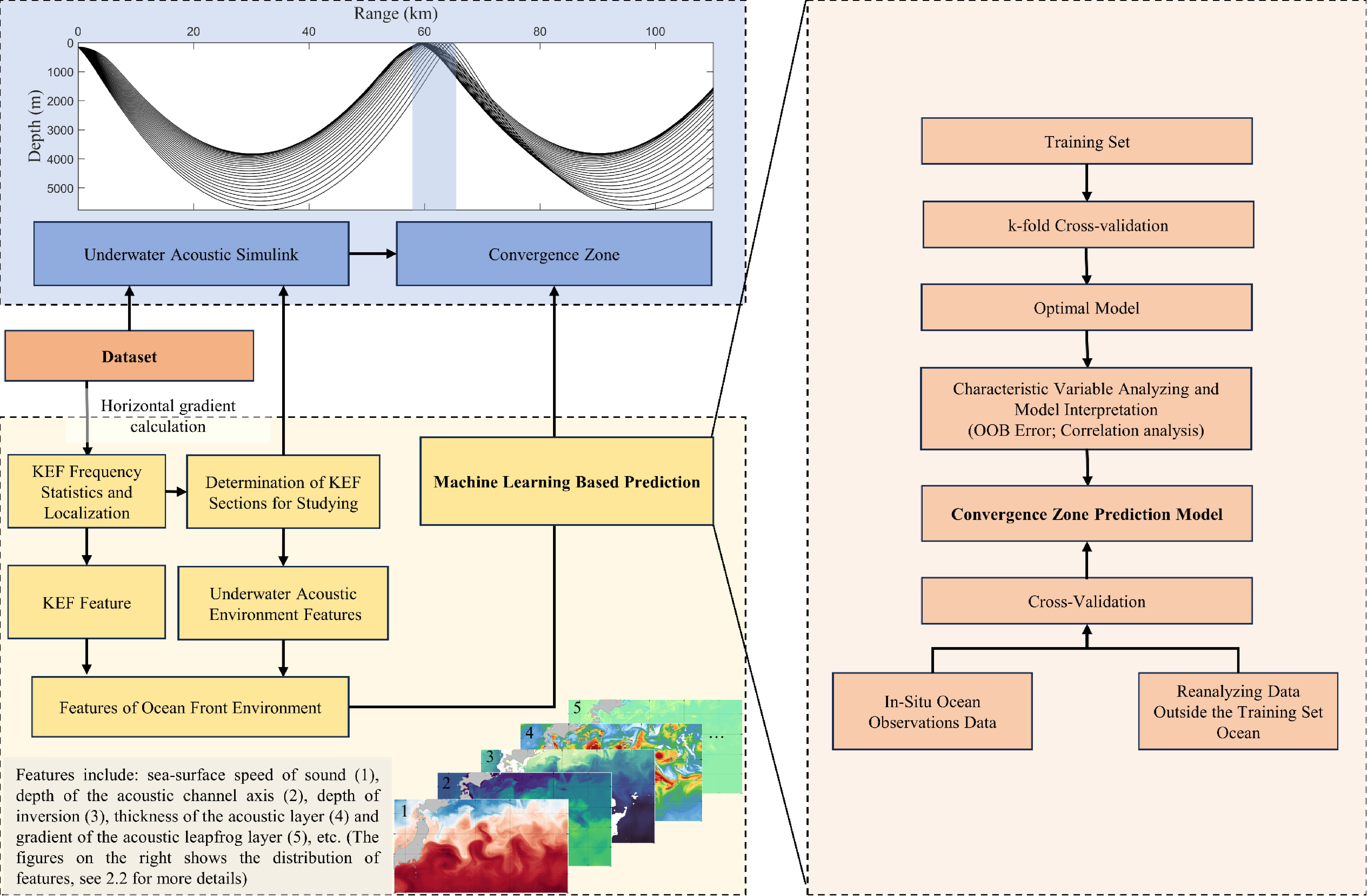
Figure 1 Flow of predictive model building for clustered areas.
Due to spatial limitations, the predictive model primarily focuses on the CZ waveguide propagating outward from the sound source in the frontal zone. Notably, the current methodology does not encompass the waveguide propagating from outside to inside the frontal zone, although the methodology remains applicable for future considerations.
The northwestern Pacific Ocean’s Kuroshio Extension (KE) has gained significant attention in recent research due to its unique geographic features and dynamic oceanic processes (Qiu et al., 2014). This region stands out as a notable source of marine energy and exhibits extensive biogeochemical cycling, rendering it an area of great scientific interest. The KE area not only serves as a significant source of marine and airborne energy (Zhou and Cheng, 2022; Yu et al., 2023)but also facilitates rich biogeochemical cycling (Tozuka et al., 2022). Consequently, this subject has been a focus of intense research in recent years. The transition zone where high-temperature, high-salinity KE waters mix with low-temperature, low-salinity pro-tides, known as KEF (Xi et al., 2022), represents one of the most significant mesoscale phenomena in the northwestern Pacific. Our study delves into the CZ waveguide within the KEF environment, employing high-resolution re-analysis JCOPE2M (Japan Coastal Ocean Predictability Experiment 2 Modified) data from the Japan Agency for Marine-Earth Science and Technology (JAMEST). This dataset offers a daily temporal resolution, 1/12° horizontal resolution, and encompasses 46 σ-layers (Miyazawa et al., 2017; Miyazawa et al., 2019). The dataset used in this study was obtained by assimilating multiple sources of information, including in-situ observations and high-resolution satellite data. This series of data has been widely utilized in the investigation of mesoscale phenomena and flow fields in the Kuroshio basin (Chang et al., 2018; Liu et al., 2019; Zheng et al., 2023).
For topographic information, our study utilized data from ETOPO1, a comprehensive seafloor topographic model with a 1′× 1′ grid size, released by the National Geophysical Data Center (NGDC) and the National Oceanic and Atmospheric Administration (NOAA). This model amalgamates global land topography and ocean depth data, drawing from numerous correlation models and specific regional measurements (Amante and Eakins, 2009), primarily derived from the Scripps Institution of Oceanography (SIO), USA, for oceanic bathymetry and GTOPO30 for global land topography. The study area, delineated by oceanic front frequency statistics, spans 146°-150°E and 35°-37°N, as depicted in Figure 2.
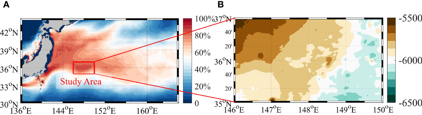
Figure 2 Overview of the study area: (A) Relative frequency of the occurrence of oceanic fronts (discrimination criterion 0.1 (m/s)/km, depth 300 m); (B) Water depth in the study area.
In-situ observations for model cross-validation were obtained from the KE System Study (KESS), an extensive observational program funded by the National Science Foundation. KESS, involving collaborations among the University of Rhode Island, the University of Hawaii, and the Woods Hole Oceanographic Institution, aims to discern and quantify the kinetic and thermodynamic processes governing the variability and interplay between the KE and its recirculating eddies (Donohue et al., 2008). Within this project, five continuous sections highlighting prominent KEF characteristics were identified using CTD data from an in-situ oceanographic survey conducted by the Research Vessel Melville in June-July 2006 as part of this initiative.
Oceanic fronts cause substantial changes in the underwater acoustic environment, resulting in notable shifts in attributes such as sound channel depth, acoustic layer thickness, and surface sound velocity on either side of the front (Etter, 2013). This study considers six specific categories of oceanic underwater acoustic environmental characteristics, evaluating features 2 through 6 both within and outside the frontal zone. Consequently, the CZ prediction model comprises 11 input features, detailed and calculated as follows:
(1) Horizontal Sound Speed Gradient (HSSG): This is defined as the ratio of the variance in sound speed at the same depth as the horizontal distance separating sites within and beyond the front, measured in (m/s)/km.
(2) Surface Sound Speed (SSS): The speed of sound at a site’s sea surface, recorded in m/s.
(3) Sound Channel Axis Depth (SCAD): Represents the depth where the sound speed reaches its minimal value, expressed in meters.
(4) Sonic Layer Depth (SLD): The deepest point in seawater where the sound velocity gradient remains positive near the surface, expressed in meters.
(5) Transition Layer of Sound Speed: The vertical sound speed gradient existing between the sound channel axis and the sonic layer, quantified in (m/s)/m.
(6) Turning Depth (TD): The depth at which the sound ray undergoes inversion below the sound channel axis. The sound speed at the TD (ci) complies with the subsequent Equation 1, where c0 denotes the sound velocity at the origin point, and αi represents the emission angle.
This research distinguishes the CZ by considering the initial CZ’s width and the separation from the origin, taking into account the ocean front’s magnitude and its range of influence. The Bellhop ray model, rooted in geometric and physical transmission principles, encompasses various ray types, including Gaussian beams(Porter, 2011). Yang et al. (2018) determined that the Bellhop model closely matches the recorded CZ distances in precise underwater acoustic examinations. Hence, it is utilized for simulating underwater acoustic propagation in this context, using the modeled CZ distances and expanses as prediction model outputs. A prerequisite for establishing a CZ is not only the existence of a sound speed’s minimal value but also the assurance that the emitted sound waves, at a minimum horizontally, are capable of reverting on the seafloor plane. This necessity stipulates that the sound speed of seawater at the boundary of the seafloor is represented as cn, as shown in Equation 2.
It is pertinent to note that, among numerous sound waves projected from a non-directional source, only those contributing to the CZ sound field are considered significant. This consideration allows determining the maximal emission angle required from the sound source for CZ formation, obtained as Equation 3.
When a sound line of encounters the seafloor, it undergoes reflection, leading to seafloor reflection propagation.
(1) Convergence Zone Distance (CZ Distance).
The CZ distance is typically defined as the cyclical distance from the 0° swept angle sound line reversal point due to the presence of focal dispersion lines near this point (Ma et al., 2023). To minimize the influence of surface waveguides, the sound source is positioned 150 m beneath the sea surface within the frontal zone. The CZ distance, measured in kilometers, is the horizontal distance from the source to the first CZ created by the source’s horizontally reversed acoustic rays.
(2) Convergence Zone Width (CZ Width).
Additionally, significant differences in CZ distances result from the large disparities in swept angles depicted in Figure 1. To establish consistent criteria and enhance prediction precision, this research computes the CZ distances for emission angles of 0° and θ, using the disparity as the CZ’s width in kilometers. The Bellhop model parameters, including the sound source parameter, are detailed in Table 1, which also lists the acoustic parameters of the seafloor substrate, taken from Hamilton (1980).
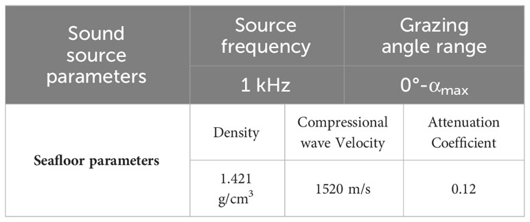
Table 1 Bellhop ray model parameter settings.
Evaluation metrics for model performance encompass mean absolute error (MAE), mean absolute percentage error (MAPE), root mean square error (RMSE), and accuracy. It is crucial to highlight that accuracy serves as a predominant measure in classification tasks. In this study’s context, accuracy represents the ratio of predicted values within a specified range of true values to the total samples. This definition is pivotal as it underscores the predictive capacity of the convergence zone feature model, establishing it as a significant indicator within our research. Lower MAE, MAPE, and RMSE values, coupled with higher accuracy, signify reduced variance between the model’s predictions and actual values, indicating superior predictive ability. The calculation methods for these indicators are illustrated in Equations 4–7.
where, “y” represents the original value of the CZ prediction, ascertained through Bellhop model simulation, while “ “ denotes the predicted value, i.e., the CZ characteristics derived from the prediction model.
This research employs 24 distinct regression algorithms to predict CZ, with their principal parameter configurations outlined in Table 2. Focusing on the waveguide of CZ, where the sound source originates in the frontal zone and progresses southward, the extracted feature dataset is divided into training, validation, and test sets at an 8:1:1 ratio before commencing sample training. Normalization of features is applied to expedite model convergence and improve feature interpretability. Additionally, alongside the 17 individual models detailed in Table 2, this study introduces 7 integrated learning strategies by combining two individual models, determining their output weights based on accuracy assessment metrics. Integrated learning strategies, through weighted model combinations, generally exhibit superior generalization performance compared to individual models.
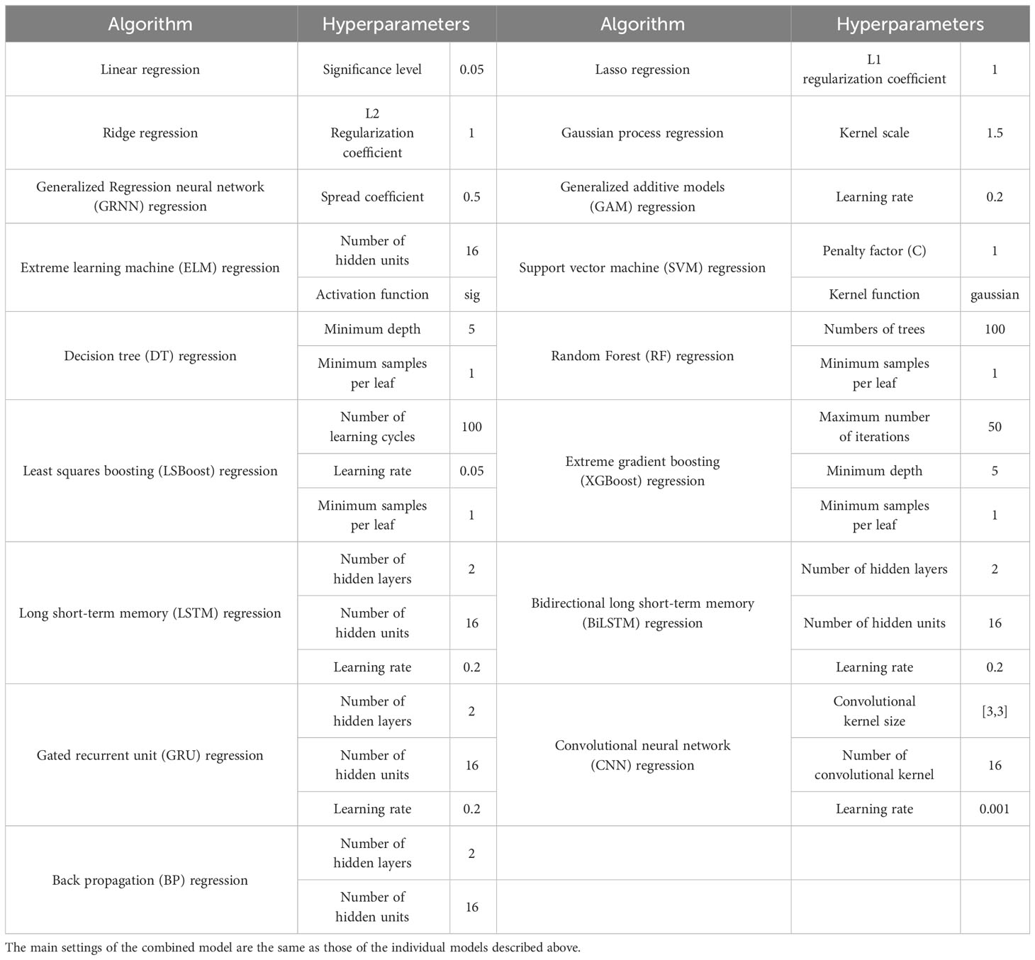
Table 2 Multiple regression model with the main parameter settings.
Subsequently, the 30a dataset is divided into ten segments using k-fold cross-validation, each containing approximately 1095 samples of 3a. From each segment, designated 3a samples form the test set, preceding 3a samples create the validation set, and the remaining 24a serve as the training set. The model undergoes training using the training set and testing with the test set, iterating this process ten times. The average outcomes from the ten models establish the final benchmark for assessing generalization accuracy, calculated using Equation 8.
where Ei is the model evaluation index observed throughout each training iteration. Post-training and evaluation, accuracy results are depicted in Figure 3. It is observed that conventional regression methods produce inferior results, often exhibiting MAPE exceeding 5%. Conversely, integrated learning strategies, assigning weights to samples and learners, demonstrate significantly improved generalization performance compared to individual learners. Specifically, integrated learning combined models such as MLP-RF and MLP-DT achieve an accuracy (1 km) surpassing 81%.

Figure 3 Comparison of the predictive accuracy of the models.
Considering the influential parameters in deep learning affecting performance, this study combines the Sparrow Search Algorithm (Xue and Shen, 2020) with four specific single deep learning network structures from Table 3 to predict the convergence zone distance within a defined hyperparameter space. The CNN hyperparameters are set as follows: number of feature maps (1-100) and stride (1-10); while the LSTM, GRU, and BiLSTM hyperparameters are set as: number of hidden layers (1-10), number of hidden units (1-100), and dropout rate (0.001-0.5). While there is an observed improvement in predictive accuracy after optimization for these algorithms, the overall enhancement is not substantial. Despite deep learning’s widespread application in numerous domains(Rajendra Kumar and Manash, 2019), in this study, due to limited features and data volume, its predictive accuracy lags behind other models. Consequently, after evaluating four metrics, MLP-RF is chosen as the optimal algorithm for predicting convergence zone features in this study. This model demonstrates high efficacy, with an average prediction error of less than 1 km in 82.16% of cases after K-fold cross-validation.
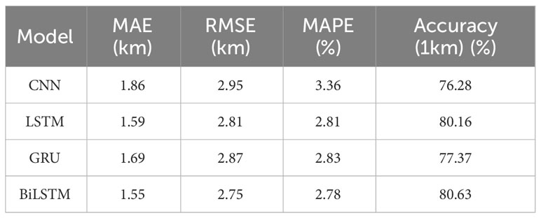
Table 3 Assessment of the predictive accuracy of convergence zone distance based on SSA and deep learning methods.
The initial step involves segmenting the complete dataset into training, validation, and test sets. The training set is utilized independently to train both the MLP (a feed-forward neural network comprising multiple neurons and layers designed for nonlinear relationship handling and complex feature learning) and the RF model (an ensemble learning algorithm with numerous decision trees, providing final predictions via voting or averaging of base classifier predictions). To enhance model performance, this study introduces distinct hyperparameter selection spaces. These models are then trained on the training set and evaluated on the validation set. This iterative process occurs within the hyperparameter space to identify the best model configuration, optimizing predictive accuracy. The Mean Absolute Error (MAE) is calculated to determine the weights of the combined MLP-RF model, using specific hyperparameter configurations detailed in Table 4.
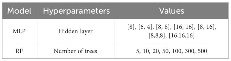
Table 4 Hyperparameter selection space for MLP-RF.
In cases where significant algorithmic differences between the models arise from the validation set, the accuracy of the combined model is expected to be intermediate. Hence, a threshold value θ (θ = 0.1) is established. If the model variation exceeds this threshold, the combination is discarded, favoring the model with the lower error as the final choice. However, if the error differential between the models falls below a specific threshold, they are merged with respective weights. The final prediction is the weighted sum of predicted values from both models, as defined in Equation 9.
where Y is the distance to the CZ predicted by different models, and W is the weight of the model, and W is the calculation method. The MLP-RF model building process is shown in Figure 4.
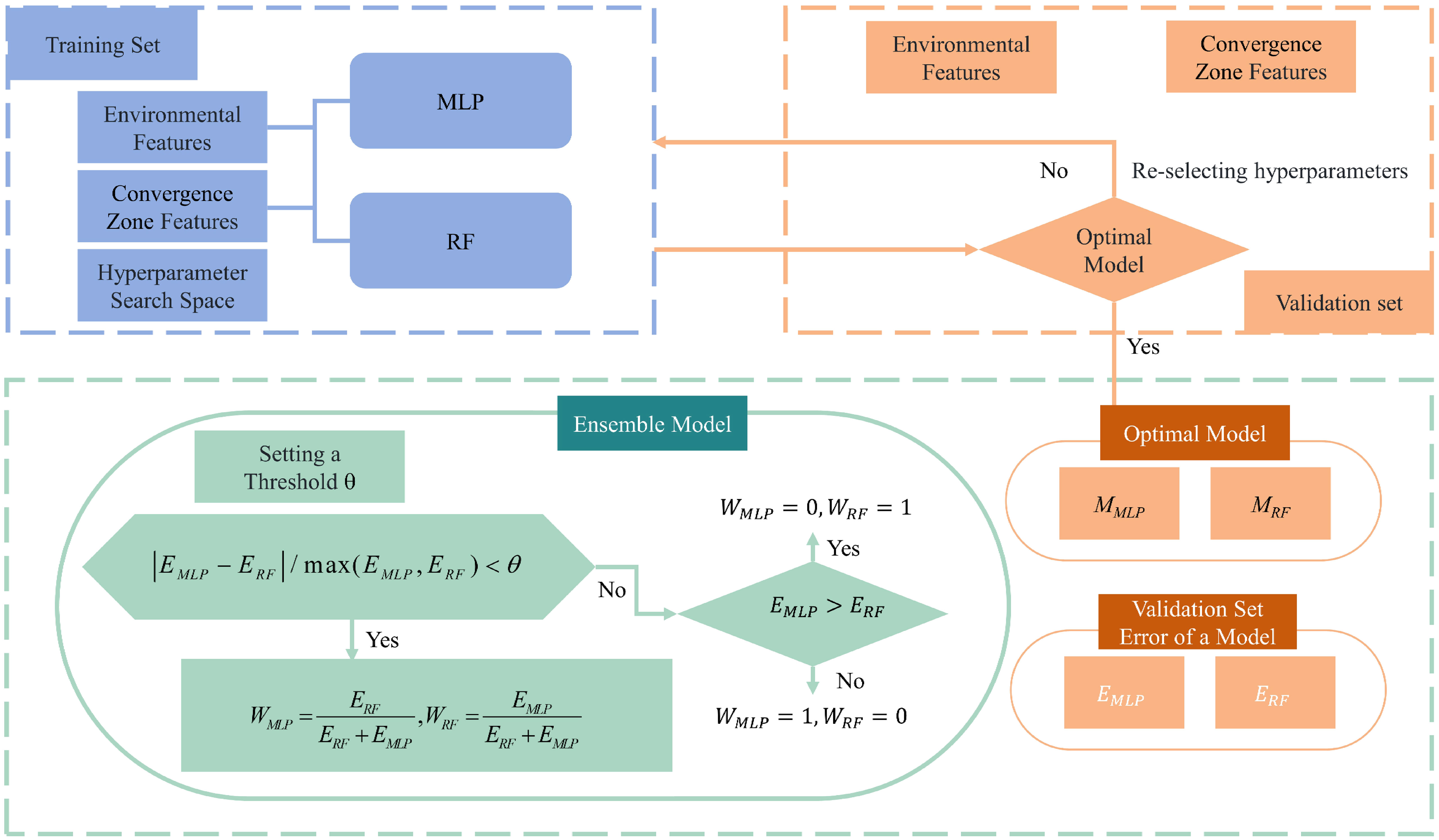
Figure 4 MLP-RF model construction process.
After multiple prediction cycles, the optimal parameters for the prediction model are determined: the MLP employs hidden layers set at [8,8] with a prediction weight of 0.51, while the RF model utilizes 300 random trees with a prediction weight of 0.49.
Given that the extracted marine features might not exhibit linear correlation with CZ features, this study utilizes Spearman correlation to analyze the mutual influence between each element. Furthermore, the Random Forest algorithm is employed to assess the relative importance of feature variables using the out-of-bag (OOB) error. This method enables the determination of how much each marine feature impacts CZ characteristics through hypothetical sampling and superimposed noise, gauging the influence of each marine feature on CZ features (Mitchell, 2011).
This analysis involves the calculation of the horizontal sound velocity gradient between two points within each water layer in the study area. Subsequently, it illustrates the correlation between the sound velocity gradient and the distance to each water layer’s CZ, as shown in Figure 5A. Notably, within the 100- to 600-m range, the intensity of KEF significantly surpasses that of other water layers. Simultaneously, the correlation between the horizontal sound velocity gradient and the distance to the CZ typically demonstrates an initial increase followed by a decrease, peaking at 150 m—a depth directly associated with the selected sound source. Consequently, the 150-m horizontal sound velocity gradient, both inside and outside the frontal zone delineated by 1°, serves as a parameter representing ocean fronts. This parameter, along with others detailed in section 2.2.1, correlates with the distance to the CZ, analyzing the importance of each oceanic condition, as depicted in Figure 5B. The results indicate that TD is crucial for the distance to the CZ, contributing over 25% among the 11 feature categories, followed by SLD2 and HSSG at 11% and 9%, respectively.
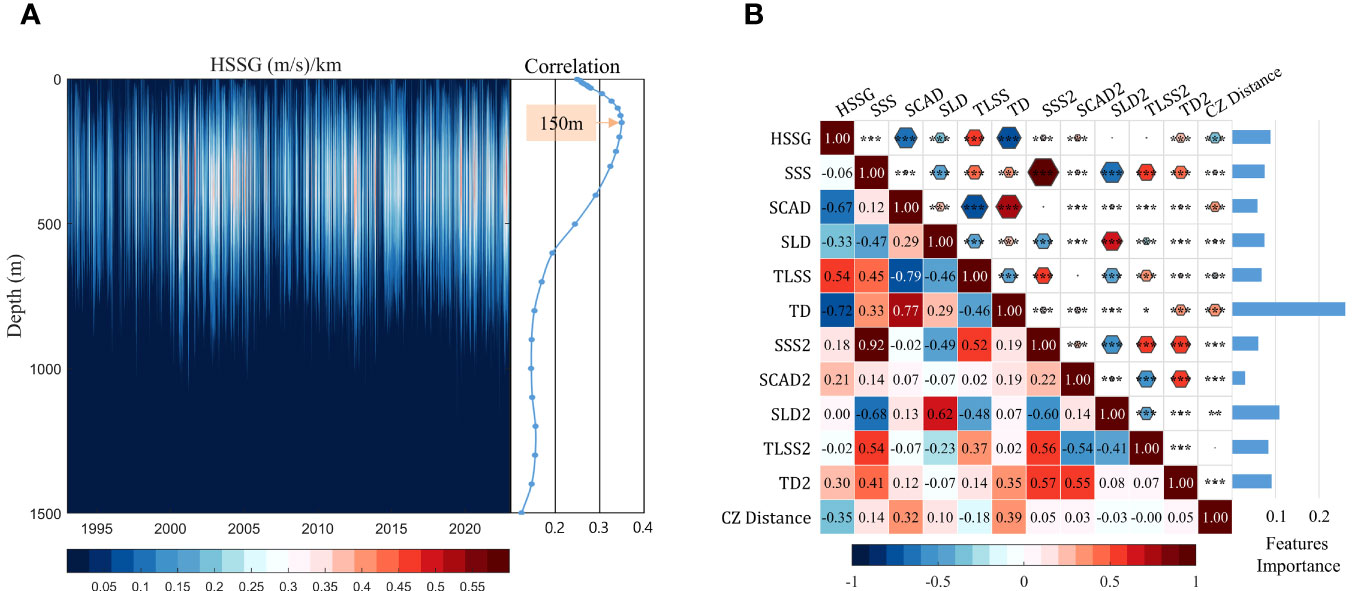
Figure 5 (A) Plot of KEF intensity versus depth and correlation with distance from the convergence zone; (B) Plot of the correlation between the marine environment and distance from the convergence zone and significance of features (*** for 99.9% significance test, ** for 99% significance test, * for 95% significance test, sites marked with “2” in the oceanic features are outside the frontal zone, and the reverse is true for stations within the frontal zone).
Snell’s law elucidates the importance of turning depth in determining the distance to the CZ. When the source is located , the horizontal distance a sound line traverses with an initial outgoing angle from the source is expressed in integral form Equation 10.
where CZ Distance (Snell) is the horizontal distance that the sound line passes through, is the depth of the sound source, is the refractive index, and z is the turning depth. The turning depth determines the maximum depth at which the sound line bends downward and determines the horizontal distance of the convergence zone.
The distance of the CZ: When the sound source is located in the frontal zone adjacent to relatively colder water, intensified ocean fronts amplify the environmental differences on either side. This results in both a shallower acoustic channel depth (with a correlation between HSSG and SCAD of −0.67) and turning depth (correlation between HSSG and TD of −0.72) on the source’s side. This enables sound rays from the source to reach the CZ more quickly. Thus, the emitted sound rays can reach the turning depth faster, bringing the CZ closer to the source. Similarly, in this study, when the source is located at high latitudes for underwater acoustic propagation—i.e., on the warmer water side—the stronger the ocean front, the deeper the acoustic channel (correlation between HSSG and SCAD is −0.69), and the shallower the turning depth (correlation between HSSG and TD is −0.77) tends to be on the source side. This delays sound rays from reaching the turning depth and pushes the CZ further from the source.
Although turning depth plays a pivotal role in predicting the CZ, this study reveals that relying solely on turning depth cannot fully capture the oceanographic features of the cross-section during K-fold cross-validation. The resultant CZ prediction model lacks robustness; for instance, prediction accuracy dips below 70% when using years such as 1993-1995 and 2018-2020 as the test set. Contrastingly, incorporating multiple oceanic parameters offers a more comprehensive view of the cross-section. Utilizing several factors as input variables for predicting CZ distances consistently yields a prediction accuracy exceeding 80% in test sets, thus enhancing generalization.
The distance and width of the CZ between 2020 and 2022 have been predicted using the optimal model evaluated in the previous section. Due to space limitations in the graph, Figures 6A, C only depict the CZ’s distance and width for 2022, respectively. Scatter density maps for the years 2020 to 2022 are shown in Figures 6B, D. The MLP-RF-based model, utilized for CZ distance prediction, demonstrates an accuracy of 82.43% (within 1 km) and an MAE of 1.56 km. Figure 6 highlights the model’s proficiency in predicting CZ distances, aligning effectively with the CZ trend. Variations in prediction results, up to 10 km in CZ despite similar seasons, may be attributed to marine environmental factors, such as the acoustic layer impacting underwater acoustic propagation. Additionally, since this study aims to predict CZ in a specific sea area that experiences shifts with the KE jets, the model primarily adapts to the correlation between marine environmental factors and CZ characteristics. Consequently, predictive efficacy slightly diminishes when these uncertain elements heavily influence the CZ. Figure 6B illustrates that predicted distances closely match original distances, clustering near the 1:1 line, with more dispersed points at the edges.

Figure 6 (A) Comparison of the 2022 projections with the original convergence zone distances; (B) Scatter density plot between the 2020-2022 projections and the original convergence zone distances; (C) Comparison of the 2022 projections with the original convergence zone widths; (D) Scatter density plot between the 2020-2022 projections and the original convergence zone widths.
The CZ width is determined from the horizontal outgoing ray and two acoustic rays emitted at the maximum outgoing angle. Predicting these rays leads to compounded errors, resulting in a marginally lower width prediction accuracy compared to distance, at 77.10% (within 1 km) and an MAE of 1.77 km. Nevertheless, Figures 6C, D showcase the model’s ability to accommodate fluctuations in the CZ’s width, with dispersion points concentrated around the 1:1 line. Upon further evaluation, the model’s accuracy in predicting a width error of less than 3 km exceeds 90%, highlighting its practical application value.
In Section 3, the sound source is positioned in the frontal zone for underwater acoustic propagation directed south. A 3D model predicting the CZ was developed by simulating underwater acoustic propagation in four distinct directions: south, north, west, and east. A 1° cross-section in each direction was extracted, utilizing the same data retrieval method as the previous section to compile datasets on marine environmental and CZ features. Predictions for underwater acoustic propagation in these four directions within the KE frontal zone from 2020 to 2022 were carried out. The averaged CZ distance and width in each direction serve as the predicted CZ. Figure 7 illustrates the simulation map and the predicted CZ using the machine learning model, depicted by two red solid lines and a red fill with 0.5 transparency, contrasted against the Bellhop3D model’s simulation results. The sound field environment mirrors that of the 2D section, with a focal depth of 150 m and the circle’s center as the central point, fixed at a display depth of 150 m. The primary CZ is identified as the circular region with low propagation loss surrounding the circle’s center. This study affirms the machine learning-based approach’s efficacy in accurately predicting the 3D CZ, exhibiting a high degree of overlap between the predicted and simulated zones.
Figure 7 Comparison of machine learning–based 3D convergence zone prediction and simulation results (labels in the upper left corner are date and sound source location).
The evaluation of CZ characteristics in four directions focused on predicting accuracy using five evaluation metrics (Table 5). Results demonstrated improved performance in CZ prediction across all directions. Specifically, distance prediction accuracy (1 km) consistently exceeded 70%, with accuracy (3 km) consistently surpassing 80%. Regarding width prediction, accuracy (1 km) typically exceeded 60%, while accuracy (3 km) consistently went beyond 80%. Remarkably, the highest accuracy was observed when the sound source directed southward, aligning with the KEF’s near parallelism to the latitude line and its northward inclination (Wang et al., 2020). This study strategically positioned the sound source cloth at the critical KEF location, significantly enhancing model interpretability. By deriving ocean environment features from the physical structure of ocean fronts, the prediction accuracy for the southward-propagating CZ model outperformed the other three directions. This resulted in a maximum accuracy increase of 8.43% for distance prediction (1 km) and 16.42% for width prediction (1 km).
Table 5 Assessment of the predictive accuracy of convergence zone features in four directions.
Predictive models constructed within an ocean front environment, incorporating specified inputs and consistent environmental features, should exhibit robust generalization capabilities. To broaden the model’s applicability, ocean data from in situ observations and neighboring sea areas were integrated as a new test set for cross-validating the CZ prediction model.
To address uncertainty regarding the precise location of in-situ observation data, adjustments were made to the feature extraction method. This involved placing the sound source cloth at the initial observation site near the section’s northern edge and utilizing acoustic profile information from the section’s final site to extract out-of-frontal features. The dataset created for predicting in-situ observations significantly deviates from this study’s original training set, with a maximum distance of nearly 190 km between in-front and out-of-front stations, compared with approximately 110 km in the training set. Despite these discrepancies and a specific anomaly in data collection direction, the proposed predictive model maintains its efficacy. Figures 8A, B illustrate the correlations between site distribution and in-situ observation prediction outcomes, indicating the model’s proficiency in delineating CZ distance trends. Prediction errors for cross sections 2-5 range between 0 and 3 km, while cross-section 1 experiences an approximate 4-km error due to substantial directional and distance deviations from the training set.
Figure 8 (A) Five cruises of the KESS project during June-August 2006 (the bottom panel shows the sound speed in m/s on June 8); (B) comparison of the original convergence zone distances of the five cruises with the results of the model prediction; (C) schematic representation of the location of cross-validation sea area I; (D) line graph of the distance of the original convergence zones in the sea area I in 2022 compared with the results of the model prediction; (E) schematic representation of the location of cross-validation sea area II; and (F) line graph of the distance of the original convergence zones in sea area II in 2022 compared with the results of the model prediction.
The structural similarity of ocean fronts theoretically allows machine learning-based CZ prediction methods to be applicable in all ocean front environments under deep-sea conditions. To further validate the universality and stability of the model, this study employed two sea areas as cross-validation regions. Cross-validation area I lies outside the training area of the Kuroshio Extension (150°-154°E, 35°-37°N) and aims to verify whether the trained model can be applied to similar sea areas. Cross-validation area II, the sub-Arctic front area (146°-150°E, 39°-41°N) (Kida et al., 2015), aims to verify the method’s applicability to ocean front regions with thermohaline structures and influence depths differing from the Kuroshio Extension Front. The network trained in the Kuroshio Extension training area in section 4.1 was used to predict the convergence zone distance in sea area I for the year 2022 (Figures 8C, D). Results showed that the predictive model effectively captured the variation trend of the convergence zone distance. Although there are differences between the ocean front characteristics in sea area II and the Kuroshio Extension Front, this study utilized the MLP-RF algorithm to predict the convergence zone distance based on extracted sub-Arctic frontal ocean features (Figures 8E, F). This achieved excellent results with an MAE of 1.28 km and an accuracy (1 km) of 86.6%, further confirming the practicality and robustness of this convergence zone prediction method.
In this investigation, high-resolution 30a reanalysis data was utilized to examine a 1° cross-section spanning from inside to outside of the frontal zone within a deep-sea area known for frequent ocean front occurrences. Out of 24 machine learning algorithms assessed, the most accurate models successfully learned and predicted six classes, 11 marine environmental features, and two CZ features. The findings highlighted the pivotal role of turning depth in the CZ prediction model, contributing over 25% according to OOB error, followed by SLD2 and HSSG at 11% and 9%, respectively. This study sheds light on the critical significance of turning depth in understanding the characteristics of the CZ within ocean front environments, employing fundamental principles of ray acoustics. Specifically, the study elucidates that a stronger or weaker ocean front, when the sound source is on the colder water side, impacts the CZ’s proximity to or distance from the sound source. Conversely, when the source is on the warmer water side, a stronger or weaker ocean front pushes the CZ farther from or nearer to the sound source.
The MLP-RF algorithm, identified as the most accurate through K-fold cross-validation, was employed to build the CZ prediction model. This model exhibited an 82.43% accuracy in predicting the CZ within a 1 km error margin in the 2D section, alongside an MAE of 1.56 km. While slightly less precise in predicting the CZ width, the model achieved a 77.1% accuracy for errors under 1 km, with an MAE of 1.77 km. Application of this model to the 3D marine environment showed promising alignment between predicted and simulated CZ, with notably higher accuracy observed for CZ propagation toward the south compared with other directions. Furthermore, the model’s performance was evaluated against in-situ ocean data and reanalysis data from adjacent ocean areas through cross-validation, demonstrating its ability to accurately predict trends in new datasets, thus confirming its robust performance and generalizability.
Given the absence of long-term sound field measurements in the marine environment, this study primarily relies on reanalysis data and ray models to predict the CZ, potentially resulting in deviations from actual conditions. However, the model construction approach suggested here is adaptable to information obtained from in-situ observations, highlighting machine learning’s ability to effectively capture the nonlinear relationship between the marine environment and the CZ in underwater acoustic predictions, offering significant practical potential. Future research should consider exploring integrating marine environment numerical predicting and physical ocean front modeling into the machine-learning prediction model to enhance its applicability and interpretability.
The original contributions presented in the study are included in the article/Supplementary Material. Further inquiries can be directed to the corresponding author.
WX: Data curation, Investigation, Methodology, Software, Visualization, Writing – original draft. LZ: Conceptualization, Methodology, Writing – review & editing. HW: Conceptualization, Funding acquisition, Project administration, Writing – review & editing.
The author(s) declare financial support was received for the research, authorship, and/or publication of this article. This project was funded by the North Pacific Deep Sound Zoning Study (DJYSYF2020-008) and Scientific Research and Development Fund of Dalian Naval Academy.
The authors express their sincere gratitude to the Japan Agency for Marine-Earth Science and Technology for their support in providing the JCOPE2M data (https://www.jamstec.go.jp/jcope/htdocs/distribution/index.html), particularly to Mr. RuoChao Zhang for his assistance with processing of the JCOPE2M data. The authors are also grateful to the NGDC, NOAA, and KESS for providing bathymetric data (https://www.ncei.noaa.gov/products/etopo-global-relief-model) and in situ data (https://uskess.whoi.edu/). The authors also acknowledge the reviewers for their constructive comments, which have improved the paper.
The authors declare that the research was conducted in the absence of any commercial or financial relationships that could be construed as a potential conflict of interest.
All claims expressed in this article are solely those of the authors and do not necessarily represent those of their affiliated organizations, or those of the publisher, the editors and the reviewers. Any product that may be evaluated in this article, or claim that may be made by its manufacturer, is not guaranteed or endorsed by the publisher.
Amante C., Eakins B. W. (2009). ETOPO1 arc-minute global relief model: procedures, data sources and analysis. NOAA Tech. memorandum NESDIS NGDC 24, 1–19. doi: 10.7289/V5C8276M
Chang Y.-L. K., Miyazawa Y., Béguer-Pon M., Han Y.-S., Ohashi K., Sheng J. (2018). Physical and biological roles of mesoscale eddies in Japanese eel larvae dispersal in the western North Pacific Ocean. Sci. Rep. 8 (1), 1–11. doi: 10.1038/s41598-018-23392-5
Chen X., Hong M., Zhu W., Mao K., Ge J., Bao S. (2019). The analysis of acoustic propagation characteristic affected by mesoscale cold-core vortex based on the UMPE model. Acoustics Aust. 47 (12), 33–49. doi: 10.1007/s40857-019-00149-2
Chen C., Yang K., Duan R., Ma Y. (2017). Acoustic propagation analysis with a sound speed feature model in the front area of Kuroshio Extension. Appl. Ocean Res. 68 (5), 1–10. doi: 10.1016/j.apor.2017.08.001
Doan V.-S., Huynh-The T., Kim D.-S. (2020). Underwater acoustic target classification based on dense convolutional neural network. IEEE Geosci. Remote Sens. Lett. 19, 1–5. doi: 10.1109/LGRS.2020.3029584
Donohue K. A., Watts D. R., Tracey K. L., Wimbush M. H., Park J.-H., Bond N. A., et al. (2008). Program studies the kuroshio extension. Eos Trans. Am. Geophysical Union (New York: CRC Press) 89, 161–162. doi: 10.1029/2008EO170002
Hamilton E. L. (1980). Geoacoustic modeling of the sea floor. J. Acoustical Soc. America 68 (5), 1313–1340. doi: 10.1121/1.385100
Hanrahan J. J. (1987). Predicting Convergence Zone Formation in the Deep Ocean, Progress in Underwater Acoustics (Boston, MA: Springer), 361–370.
Kida S., Mitsudera H., Aoki S., Guo X., Ito S.i., Kobashi F., et al. (2015). Oceanic fronts and jets around Japan: a review. J. Oceanography 71, 469–497. doi: 10.1007/978-4-431-56053-1_1
Lagrois D., Bonnell T. R., Shukla A., Chion C. (2022). The gradient-boosting method for tackling high computing demand in underwater acoustic propagation modeling. J. Mar. Sci. Eng. 10 (7), 899. doi: 10.3390/jmse10070899
Lin Y., Zhu M., Wu Y., Zhang W. (2020). “Passive source ranging using residual neural network with one hydrophone in shallow water,” in 2020 IEEE 3rd International Conference on Information Communication and Signal Processing (ICICSP), Shanghai, China. 122–125 (IEEE).
Liu Y., Meng Z., Chen W., Liang Y., Chen W., Chen Y. (2022). Ocean fronts and their acoustic effects: A review. J. Mar. Sci. Eng. 10 (12), 2021. doi: 10.3390/jmse10122021
Liu Z. J., Nakamura H., Zhu X. H., Nishina A., Guo X., Dong M. (2019). Tempo-spatial variations of the Kuroshio current in the Tokara Strait based on long-term ferryboat ADCP data. J. Geophysical Research: Oceans 124 (8), 6030–6049. doi: 10.1029/2018JC014771
Liu J., Piao S., Gong L., Zhang M., Guo Y., Zhang S. (2021). The effect of mesoscale eddy on the characteristic of sound propagation. J. Mar. Sci. Eng. 9 (8), 787. doi: 10.3390/jmse9080787
Ma S., Guo X., Zhang L., Lan Q., Huang C. (2023). Riemannian geometric modeling of underwater acoustic ray propagation · Application——Riemannian geometric model of convergence zone in the deep ocean. Acta Physica Sin. 72 (4), 108–120. doi: 10.7498/aps.72.20221495
Mccarthy R. A., Merrifield S. T., Sarkar J., Terrill E. (2023). Machine learning of acoustic propagation models for sound aware autonomous systems. J. Acoustical Soc. America 153 (3_supplement), A175. doi: 10.1121/10.0018570
Mitchell M. W. (2011). Bias of the random forest out-of-bag (OOB) error for certain input parameters. Open J. Stat 1 (3), 205–211. doi: 10.4236/ojs.2011.13024
Miyazawa Y., Kuwano-Yoshida A., Nishikawa H., Narazaki T., Fukuoka T., Sato K. (2019). Temperature profiling measurements by sea turtles improve ocean state estimation in the Kuroshio-Oyashio Confluence region. Ocean Dynamics 69 (2), 267–282. doi: 10.1007/s10236-018-1238-5
Miyazawa Y., Varlamov S. M., Miyama T., Guo X., Hihara T., Kiyomatsu K., et al. (2017). Assimilation of high-resolution sea surface temperature data into an operational nowcast/forecast system around Japan using a multi-scale three-dimensional variational scheme. Ocean Dynamics 67 (6), 713–728. doi: 10.1007/s10236-017-1056-1
Niu H., Gong Z., Ozanich E., Gerstoft P., Wang H., Li Z. (2019). Deep-learning source localization using multi-frequency magnitude-only data. J. Acoustical Soc. America 146, 211–222. doi: 10.1121/1.5116016
Ozanich E., Gawarkiewicz G. G., Lin Y.-T. (2022). Study of acoustic propagation across an oceanic front at the edge of the New England shelf. J. Acoustical Soc. America 152 (6), 3756–3767. doi: 10.1121/10.0016630
Porter M. B. (2011). The bellhop manual and user’s guide: Preliminary draft. Heat, Light, and Sound Research (CA, USA: Inc., La Jolla). Tech. Rep 260.
Qiu B., Chen S., Schneider N., Taguchi B. (2014). A coupled decadal prediction of the dynamic state of the kuroshio extension system. J. Climate 27 (4), 1751–1764. doi: 10.1175/JCLI-D-13-00318.1
Rajendra Kumar P., Manash E. B. K. (2019). Deep learning: a branch of machine learning. J. Physics: Conf. Ser. 1228 (1), 12045. doi: 10.1088/1742-6596/1228/1/012045
Shafiee Sarvestani R. (2022). Acoustic propagation analysis in the front of saline water mass in the Gulf of Aden. J. Oceanography 13 (50), 45–58. doi: 10.52547/joc.13.50.45
Tozuka T., Sasai Y., Yasunaka S., Sasaki H., Nonaka M. (2022). Simulated decadal variations of surface and subsurface phytoplankton in the upstream Kuroshio Extension region. Prog. Earth Planetary Sci. 9, 1–14. doi: 10.1186/s40645-022-00532-0
Wang J., Mao K., Chen X., Zhu K. (2020). Evolution and structure of the kuroshio extension front in spring 2019. J. Mar. Sci. Eng. 8 (7), 502. doi: 10.3390/jmse8070502
Wu S., Li Z., Qin J., Wang M., Li W. (2022). The effects of sound speed profile to the convergence zone in deep water. J. Mar. Sci. Eng. 10 (3), 424. doi: 10.3390/jmse10030424
Wu S., Qin J., Li Z. (2023). Effect of sound speed profile on the structure of acoustic pulse and the convergence zone in deep water. J. Acoustical Soc. America 154 (4_supplement), A355. doi: 10.1121/10.0023782
Xi J., Wang Y., Feng Z., Liu Y., Guo X. (2022). Variability and intensity of the sea surface temperature front associated with the kuroshio extension. Front. Mar. Sci. 9. doi: 10.3389/fmars.2022.836469
Xiao R., Lei F., Zhu H., Chen C., Xue Y. (2021). Influence of mesoscale vortex on underwater low-frequency sound propagation. J. Physics: Conf. Ser. 1739 (1), 12018. doi: 10.1088/1742-6596/1739/1/012018
Xue J., Shen B. (2020). A novel swarm intelligence optimization approach: sparrow search algorithm. Syst. Sci. Control Eng. 8 (1), 22–34. doi: 10.1080/21642583.2019.1708830
Xue R., Yang Y., Weng J., Wen H., Chen H., Lin L. (2021). Modelling convergence zone propagation under the influence of arctic front 2021 OES China ocean acoustics (COA). Harbin China, 229–233. doi: 10.1109/COA50123.2021.9520075
Yang H., Lee K., Choo Y., Kim K. (2020). Underwater acoustic research trends with machine learning: general background. J. Ocean Eng. Technol. 34 (2), 147–154. doi: 10.26748/KSOE.2020.015
Yang K., Lu Y., Xue R., Sun Q. (2018). Transmission characteristics of convergence zone in deep-sea slope. Appl. Acoustics 139, 222–228. doi: 10.1016/j.apacoust.2018.05.004
Yu P., Yang M., Zhang C., Li Y., Zhang L., Chen S. (2023). Response of the north pacific storm track activity in the cold season to multi-scale oceanic variations of kuroshio extension system: A statistical assessment. Adv. Atmospheric Sci. 40 (3), 514–530. doi: 10.1007/s00376-022-2044-z
Zhang L., Chen W.-j., Liu D.-q. (2020). Uncertain effects of linear internal waves on convergence zone propagation in deep water. J. Coast. Res. 99 (sp1), 296–309. doi: 10.2112/SI99-042.1
Zhang Y., Zhang S., Zhu F., Hu Z., Gao S., Chen Q. (2021). Effect of MODAS data on convergence zone distance prediction 2021 OES China ocean acoustics (COA). IEEE Harbin China, 148–151. doi: 10.1109/COA50123.2021.9519957
Zheng J., Guo X., Miyazawa Y., Yang H., Yang M., Mao X., et al. (2023). Diagnostic analysis of the response of volume transport through the tsushima strait to the eddy-induced variations in the kuroshio region. J. Phys. Oceanography 53 (11), 2597–2617. doi: 10.1175/JPO-D-22-0164.1
Keywords: convergence zone, machine learning, Kuroshio extension front, environmental feature extraction, multiple regression prediction
Citation: Xu W, Zhang L and Wang H (2024) Machine learning–based feature prediction of convergence zones in ocean front environments. Front. Mar. Sci. 11:1337234. doi: 10.3389/fmars.2024.1337234
Received: 14 November 2023; Accepted: 10 January 2024;
Published: 25 January 2024.
Edited by:
Haiyong Zheng, Ocean University of China, ChinaReviewed by:
Feng Gao, Ocean University of China, ChinaCopyright © 2024 Xu, Zhang and Wang. This is an open-access article distributed under the terms of the Creative Commons Attribution License (CC BY). The use, distribution or reproduction in other forums is permitted, provided the original author(s) and the copyright owner(s) are credited and that the original publication in this journal is cited, in accordance with accepted academic practice. No use, distribution or reproduction is permitted which does not comply with these terms.
*Correspondence: Lei Zhang, c3RvbmUzMzNAdG9tLmNvbQ==
Disclaimer: All claims expressed in this article are solely those of the authors and do not necessarily represent those of their affiliated organizations, or those of the publisher, the editors and the reviewers. Any product that may be evaluated in this article or claim that may be made by its manufacturer is not guaranteed or endorsed by the publisher.
Research integrity at Frontiers
Learn more about the work of our research integrity team to safeguard the quality of each article we publish.