Utilizing residual networks for remote sensing estimation of total nitrogen concentration in Shandong offshore areas

Nitrogen is one of the critical factors in water pollution and eutrophication, so applying the deep learning method in remote sensing inversion of nitrogen can provide basic information for environmental management. This paper proposes a two-step feature extraction method to solve the problem that the number of bands in water quality inversion is insufficient and the deep learning method cannot be fully exploited. Firstly, manual feature extraction is completed through the fusion between bands to obtain a set of high-latitude shallow factors, which make the features rich and diverse. Then, a one-dimensional convolutional residual network (ResNet-1D) is constructed, and the deep features are automatically extracted through convolution operations of the model, where the residual learning is used to reduce the training difficulty. The full connection is established through depth features. The comparison of models shows that the Mean Relative Error (MRE) is decreased by at least 10% in both test and validation datasets. Finally, the spatiotemporal distribution of total nitrogen concentration (TNC) in the coastal waters of Shandong is explored. In general, the spatial distribution is that the concentration near the coast is higher than the far. The temporal variation is that the monthly mean of the TNC is low in March, moderate in May and August, and high in October; the annual average value of TNC is 0.3mg/L, which has decreased slightly year by year since 2014.

1 Introduction

The deterioration of surface water quality and eutrophication has become a serious pollution problem in many countries over recent decades due to the increasing amount of nutrients discharged into water by various pollution sources (Smith et al., 1999; Yu et al., 2016). Of all nutrients, nitrogen is required to support aquatic plant growth and is the crucial limiting nutrient in most aquatic and terrestrial ecosystems (Guildford and Hecky, 2000; Conley et al., 2009). So, it is closely related to the ecological balance of aquatic organisms and eutrophication (Sagan et al., 2020). Therefore, effectively monitoring nitrogen concentration is essential for evaluating the water environment (Qin et al., 2006). Traditional water quality monitoring methods can monitor nitrogen element concentration, providing accurate and detailed water quality parameter information at monitoring points (Sun et al., 2014). Still, it is difficult to reflect the spatial distribution of water quality, and it consumes many resources (Mohammad et al., 2016).

Water quality remote sensing monitoring is a technology that uses spaceborne sensors to obtain image data, constructs a water quality parameter inversion model based on image reflectance, and calculates water environment factors (Wagle et al., 2020). It explores the internal relationship between spectral reflectance and water composition (Harvey et al., 2015). The method has the advantages of a wide range and long-term dynamics, which can make up for the shortcomings of traditional water quality monitoring methods (Shen et al., 2020). The inversion model is the core, and the data is the key to the process (Uudeberg et al., 2020). The water quality remote sensing inversion method can be divided into empirical and analytical methods. The former is widely used due to its superior accuracy and easy construction, but the universality is low (Soomets et al., 2020). Therefore, it is necessary to establish a specific empirical model suitable for the study area.

Nitrogen is not only an essential factor that contributes to the formation of bloom but also an indicator of water eutrophication (Chen, 2006). Therefore, monitoring its spatial and temporal distribution characteristics using remote sensing data is highly critical to preventing nitrogen pollution and strengthening water ecological environment governance (Muhammad et al., 2020; Muhammad et al., 2022). Compared with chlorophyll-a and total suspended solids, TN does not have significant spectral responses, making remote sensing retrieval difficult. Carpenter and Serwan constructed a linear regression model in the study area using Landsat data to invert water quality parameters (Carpenter and Carpenter, 1983; Serwan, 1993). However, linear models can only reflect the linear relationship between spectral data and water quality parameters. Due to the limitations of watercolor remote sensing detection technology and the complexity of water dynamics, the two types of data exhibit complex nonlinear relationships (Wagle et al., 2020), such as exponent, logarithm, power function, polynomial, etc (Reilly and Werdell, 2019). The above models are simple and have explicit mapping relationships, making them common methods for inverting water quality parameters (Liu et al., 2015; Li, 2020; Zhang et al., 2021). However, these methods require the sample population to have specific distribution characteristics, resulting in small applicability, low prediction accuracy, and poor generalization performance (Fang et al., 2019).

With the development of machine learning, nonparametric and nonlinear models represented by random forests (Shen et al., 2020), support vector machines (SVM) (Sheng et al., 2021), and neural networks (Zhu et al., 2017; Pahlevan et al., 2020) have the characteristics of broad applicability, high accuracy, and strong reliability and are favored by many scholars. Based on measured hyperspectral data, Liu manually selected sensitive bands and used SVM models to invert the surface TNC of rivers in arid areas (Liu et al., 2020) and so on (Dong et al., 2023; Yin et al., 2023a; Yin et al., 2023b; Wen et al., 2024). Amiri and Liu fitted the distribution of TNC in the study area using artificial neural networks and multiple linear regression methods (Amiri and Nakane, 2009; Liu et al., 2015). The results showed that the former had higher accuracy. The input factors of the above machine learning models are the original band or artificially designed combination band, and the number is relatively small. The model is calculated by these limited shallow features, with slight accuracy improvement (Song et al., 2012; Sun et al., 2023). Moreover, the spectral characteristics of nitrogen-containing water bodies are comprehensively influenced by chlorophyll, suspended solids, and colored soluble organic matter in the water. Hence, the inversion model involves multiple and complex variables (Mohammad et al., 2016).

Deep learning can automatically extract deep features and achieve complex non-linear mapping (Lecun et al., 2015). Simultaneously possessing the ability to process high-dimensional data, it is widely used in fields such as computer vision (Le, 2013), natural language processing (Li, 2018), remote sensing image classification (Marmanis et al., 2016), and remote sensing water quality parameter inversion (Yu, 2019; Han et al., 2023). Convolutional neural networks (CNN) are one of the most widely used methods in deep learning models (Zhao and Du, 2016). Pu constructed a multilayer CNN to invert water quality parameters (Pu et al., 2019). Yu first used CNN to build a global ocean Chla concentration inversion model and demonstrated its superiority in solving inversion problems (Yu et al., 2020). However, with increased depth, CNN will experience gradient explosion or disappearance, resulting in abnormal training. The residual network solves the problem that the deep network is challenging to train by adding residual learning units (He et al., 2016).

The measured hyperspectral data is adopted due to rich bands in water quality remote sensing monitoring, which can accurately capture the subtle differences between water quality parameters (Pyo et al., 2018). However, such data is challenging, expensive, and has a small coverage range. In contrast, multispectral data is widely used because of its easy acquisition, low cost, and comprehensive coverage (Mohammad et al., 2016). However, this type of data has a wide and limited number of bands, which limits its application in deep learning (Cao et al., 2020; Cao et al., 2022). So, spaceborne hyperspectral data is a perfect choice.

The sample points of TN and synchronous MODIS image data are used in the paper. The multiple original bands are fused into a set of high-dimensional feature factors through operation, which gets diverse features. The ResNet-1D is employed as the inversion model to mine the deep features between high-dimensional factors automatically. The residual learning is used to reduce the training difficulty of the network, and the remote sensing monitoring model of TNC is established. Compared with the BP, PSO-BP, and CNN models, the result shows that the MRE of the ResNet-1D is decreased by at least 10% on the two data. The temporal and spatial variation characteristic of TNC in the coastal waters of Shandong is explored.

2 Study area and data

2.1 Study area

The coastal water of the Shandong Peninsula is the research object, whose latitude and longitude range is 117° 50′ ~123°30′E, 34°50′~38°40′N, as shown in Figure 1. The mudflat in the region accounts for about 15% of the country, and the coastline starts from the Zhang Weixin River in the north and ends at the Xiuzhen River in the south, with a total length of 3345km. Over 300 rivers emptying into the sea, including the Yellow and Weihe Rivers, continuously transport fresh water and terrestrial materials to the nearshore waters. These rivers flow through different regions and carry various types of land-sourced pollutants. Consequently, the research area has been continuously injected with terrestrial materials, especially inorganic nitrogen and active phosphate, which have exacerbated the eutrophication of seawater. In addition, there are numerous aquaculture areas in the region. Human activities have intensified with the continuous development and utilization of marine resources, seriously affecting the nearshore water quality. Ecological and environmental problems are prominent, with frequent occurrences of red tide, green tide, and other disasters affecting ship traffic and marine fishery, causing substantial economic losses.

Figure 1

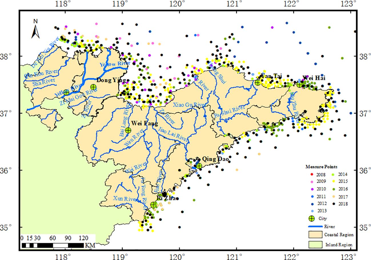
Figure 1 Research area and monitor points.

2.2 Measured data

To explore the water quality around the Shandong Peninsula, the Beihai Branch of the Natural Resources Ministry carried out continuous water quality testing from 2008 to 2018. The weather was clear during the measurement, and the water surface was calm. Water samples are collected from 10:00 to 14:00. One water sample is obtained at each monitor point, stored at a low temperature, and moved to the laboratory to measure the TNC. A total of 1276 points were received over the past 11 years. Figure 1 shows the spatial distribution of measure points, with more points near-shore than far shore and more in the northern part of the Peninsula than in the eastern and southeastern parts.

The statistics result of the measured TNC in each year is shown in Table 1, which demonstrates that the maximum TNC value is 1.47mg/L, and the minimum is 0.001mg/L, indicating a significant dispersion.

Table 1

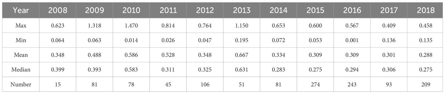
Table 1 Statistical table of measured TNC data.

Figure 2 is the boxplot of the measured TN data. The white dots in the boxes symbolize the respective mean, and the horizontal lines represent the median. The above two do not coincide in some years. The bottom and top line of each box are the 25th percentile (Q1) and 75th percentile (Q2), respectively, so that the difference between Q1 and Q2 builds the interquartile range (IQR). The bottom line of the whisker is the larger value between Q1-1.5*IQR and the minimum value of the annual measured data, and the top line of the whisker is the smaller value between Q2 + 1.5*IQR and the maximum value of the data. The points outside the whisker are treated as singular points. These points may lead to an immense loss function of the model, resulting in excessive weight adjustment and unreasonable weight value in the optimization process, which reduces the stability and generalization ability of the model. Therefore, the singularities should be deserted.

Figure 2

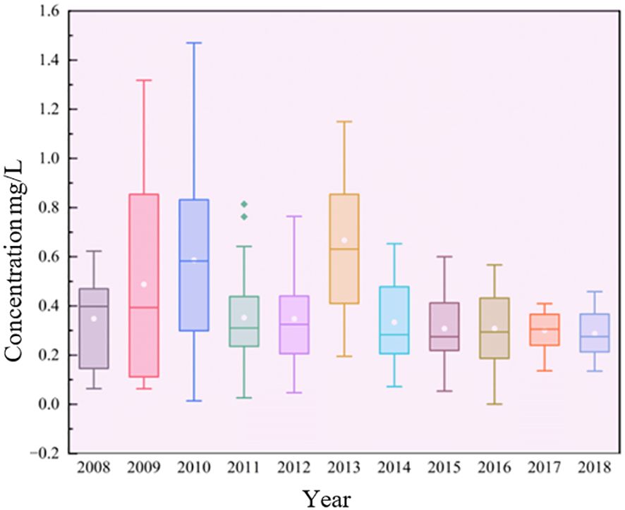
Figure 2 Box plot of measured TN data.

As shown in Figure 2, except in 2008, the median of the measured data is less than or equal to the mean value, indicating that the data number in the low-value area is more than that in the high-value area. From 2008 to 2013, the height of the box was high, and the distance between the top line and the bottom line was large. From 2014 to 2018, the height of the box was low, and the distance between the top line and the bottom line was small. This indicates that the measured data value of the latter was lower than that of the former, and the difference between the data was minor.

2.3 Satellite image data

The MODIS, SeaWiFS, MERIS, VIIRS, GOCI, COCTS, MSI, etc., are commonly used water quality remote sensing monitoring sensors, whose parameters are shown in Table 2. In contrast, MODIS has significant advantages in resolution and band number; therefore, it is used as the data source.

Table 2

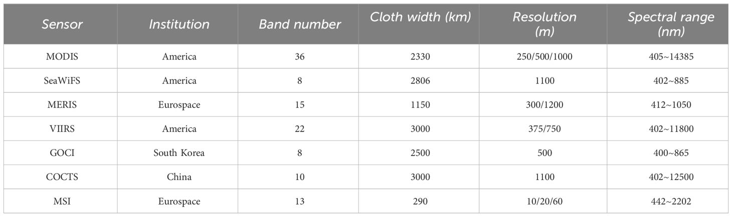
Table 2 Common sensor parameters for water quality remote sensing.

The spatial resolutions of MODIS are 250m, 500m, and 1000m, and the number of corresponding bands is 2, 5, and 29, respectively. The former has a high resolution, but the band number is small, while the latter has a large number of bands, but the resolution is too low. Considering the band number, resolution, and research area size, bands with resolutions of 250m and 500m are selected as the data sources shown in Table 3.

Table 3

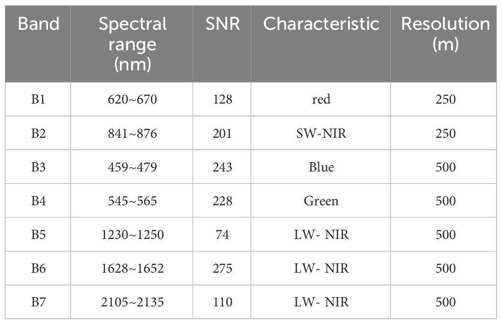
Table 3 MODIS data band information.

Considering tides, ocean currents, and so on, 43 cloudless or slightly cloudy remote sense images were downloaded based on the actual sampling date and with a time window of ± 6 hours. The image dates are shown in Table 4.

Table 4

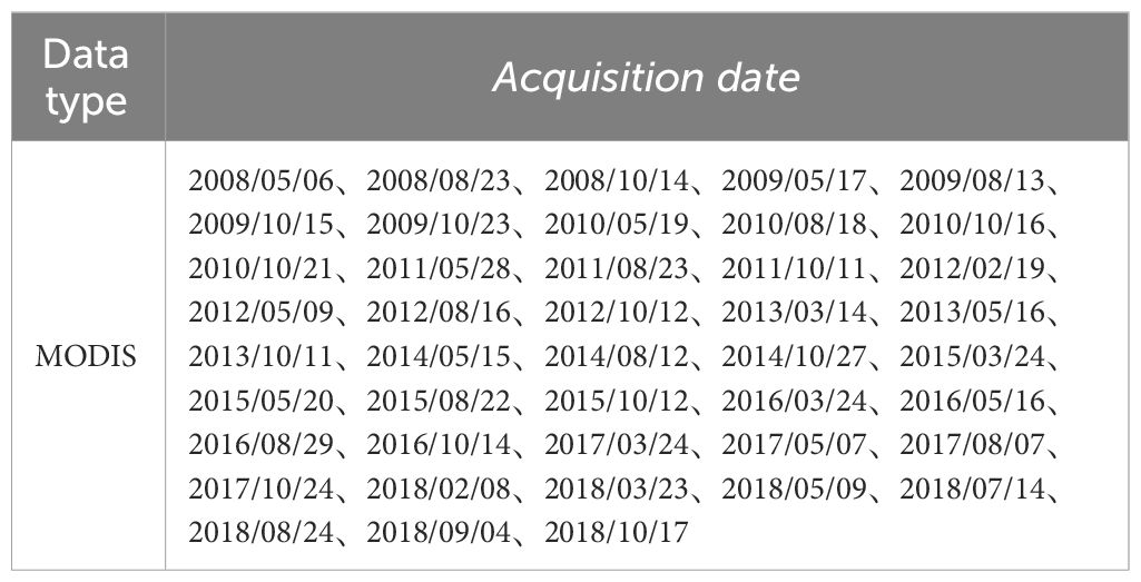
Table 4 Image date information.

To reduce the processing time, each image is cropped first. Because the measured points are located in the sea within 60 km of the coastline, a unilateral buffer is generated by extending 60km from the shoreline to the ocean. The buffer zone crops the image to retain the nearshore area only. Then, radiation calibration, geometric correction, atmospheric correction, and other preprocessing work are carried out to obtain remote sensing reflectance data. Finally, based on the spectral differences of water in the green and near-infrared bands, the Normalized Water Index (NDWI) is applied to suppress non-water interference and extract water information. The calculation formula is shown in Equation 1.

$\begin{array}{ll}\mathit{\text{NDWI}}=\frac{({\mathit{\text{ρ}}}_{GREEN}-{\mathit{\text{ρ}}}_{NIR})}{({\mathit{\text{ρ}}}_{GREEN}+{\mathit{\text{ρ}}}_{NIR})}& (1)\end{array}$

${\rho }_{GREEN}$、 ${\rho }_{NIR}$ is the pixel reflectance in the green and near-infrared band.

2.4 Data preprocess

The water quality remote sensing inversion model is inseparable from high-quality data, so the measured water TN data and the extracted image reflectance data must be preprocessed.

Due to human operational errors and instrument factors, points with the same acquisition time and close position are regarded as repeated points, and the mean value is calculated. The nutrient-rich freshwater carried by rivers flows into the sea at the estuary, and feed is used in aquaculture. So, the river estuary and aquaculture are rich in nutrients, and the measured TNC values in these areas are significantly higher, which are singular points and will be excluded (Chen et al., 2019). After preprocessing the measured points, the corresponding pixels on the image are searched based on the acquisition time and position.

The pixels of the sea-land junction in the image are mixtures due to the spatial resolution limitation. The image has several mixed pixels of clouds and water affected by weather with a composite reflectivity value. At the same time, factors such as cloud cover, astigmatism, and flares lead to low-quality pixels in the image. If the monitoring point corresponds to the above pixels in the image, there is a lack of accurate reflectance data. The above pixel points and corresponding measured points will be deleted to improve the data quality, ensuring that only high-quality pure water pixel reflectance values are used in the inversion model. To further reduce the impact of singular values, taking the pixel corresponding to the measured point as the center, the mean value of the 3×3 neighborhood pixel is calculated as the remote sensing reflectivity sample data.

After the above processing, 301 measured points are ultimately selected as the model inversion sample data. To understand the status of the sample data, indicators such as the minimum, maximum, average, and standard deviation of TNC are calculated, as shown in Table 5. We can see that the dispersion is smaller than the original data.

Table 5

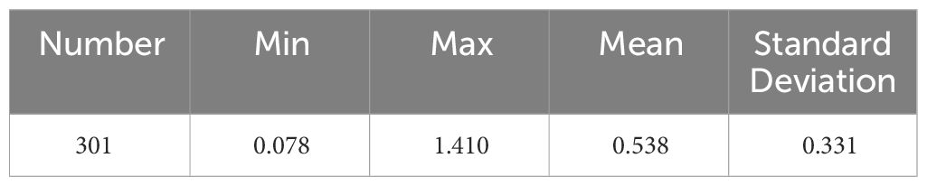
Table 5 Statistical table of sample TNC data.

3 Research methods

3.1 Correlation analysis and evaluation indicator

The band sensitivity analysis of spectral reflectance data and water quality parameter concentration data is carried out to screen out the bands or band combinations that significantly correlate with TNC. Taking them as the input factors is the premise of establishing the inversion model and improving the inversion accuracy.

The correlation coefficient (r) is a quantitative indicator that measures the linear relationship between two variables, which can be calculated through Pearson analysis, as shown in Equation 2. The value is between -1 and +1, and the larger the deal, the stronger the linear relationship. A positive value indicates a positive correlation, a negative value indicates a negative correlation, and a value of 0 indicates a non-correlation.

The coefficient of determination (R²) is an evaluation index of the agreement degree between the regression value and the actual observed value. It is used to determine the fit degree of the regression model, as shown in Equation 3. The greater the R², the higher the interpretation of the independent variable to the dependent variable. In addition, the MRE is used to evaluate the accuracy of the inversion model, as shown in Equation 4.

$\begin{array}{ll}{r}_j=\frac{{\sum }_{i=1}^n(x_{ij}-\overline{x})(y_i-\overline{y)}}{\sqrt{{\sum }_{i=1}^n{(x_{ij}-\overline{x})}^2\sum {(y_i-\overline{y})}^2}}& (2)\end{array}$

$\begin{array}{ll}{\mathit{\text{R}}}^{\mathbf{2}}=\frac{{\sum }_{i=1}^n(y_{ipre}-{\overline{y)}}^2}{{\sum }_{i=1}^n(y_i-{\overline{y)}}^2}& (3)\end{array}$

$\begin{array}{ll}\mathit{\text{MRE}}=\frac{\mathbf{1}}{\mathit{\text{n}}}{\sum }_{\mathit{\text{i}}=\mathbf{1}}^{\mathit{\text{n}}}\left|\frac{{\mathit{\text{y}}}_{\mathit{\text{ipre}}-}{\mathit{\text{y}}}_{\mathit{\text{i}}}}{{\mathit{\text{y}}}_{\mathit{\text{i}}}}\right|\times \mathbf{100}\%& (4)\end{array}$

$r_j$ is the correlation coefficient; $j$ is the band number; $n$ is the number of samples; $x_{ij}$ is the spectral reflectance of the i sample in the j band; $\overline{x}$, $\overline{y}$ is the mean of reflectance and TNC respectively; $y_i$, $y_{ipre}$ is the measured and predicted value of TNC of i sample respectively.

According to Equations 2 and 3, we can see that correlation coefficient and determination coefficient are different indicators. When two variables have a linear relationship, then ${\mathit{\text{R}}}^{\mathbf{2}}={\mathit{\text{r}}}^{\mathbf{2}}$.

3.2 One-dimensional convolutional network

CNN automatically extracts features through multilayer convolution and pooling operations. Compared with explicit feature extraction methods, the obtained deep features are more abstract and compelling, making essential breakthroughs in machine learning (Sun et al., 2023). The convolution operation can be represented by Equation 5.

$\begin{array}{ll}{v}_{i,j}^x=f\left(\sum _m\sum _{p=0}^{p_i-1}{w}_{i,j,m}^p{v}_{(i-1),m}^{x+p}+b_{i,j}\right)& (5)\end{array}$

$v_{i,j}^x$ is the value at position x in the j feature map of the i layer; f is the activation function; m is the index of layer i and i-1; $p_i$ represents the length of a one-dimensional convolutional kernel; $w_{i,j,m}^p$ is the weight of position p connected to the m feature map; $v_{(i-1),m}^{x+p}$ is the value at position x+p in the m feature map of the i-1 layer; $b_{i,j}$ is the offset on the j feature map of the i layer.

According to the dimensions of the convolutional kernel, the CNN is divided into three types: one-dimensional, two-dimensional, and three-dimensional. The reflectance data of the remote sensing image is one-dimensional spectral data, and the one-dimensional convolutional network (1D CNN) has shown promising results in analyzing spectral data, which is used in the environmental classification task (Riese and Keller, 2019) and Chl-a simulation training (Maier et al., 2021). So, it was adopted in the study. 1D CNN with a feature graph and a convolution kernel length of 3 can be represented in Figure 3.

Figure 3

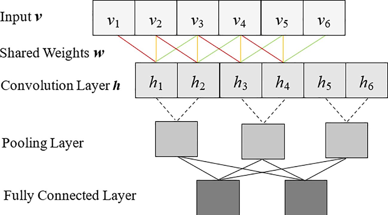
Figure 3 Structure diagram of the 1D convolution process.

3.3 Residual network

Generally speaking, the deeper the neural network is, the more abstract features are extracted, and the better the network performance will get. However, if there are too many layers in applications, the gradient explosion or disappearance may occur, making it difficult to train and optimize the network. The Residual Net (ResNet) makes it possible to train the deep network, profoundly impacting deep learning (He et al., 2016).

ResNet set up a residual module based on convolutional neural networks, composed of residual mapping and identity mapping, as shown in Figure 4. The dashed box in the figure is the residual mapping, consisting of convolutional layers, activation functions, and convolutional layers, which is the main path of the module. The curve part is the identity mapping, a shortcut that directly skips the middle part of the convolution layer and fuses with the main path. Thus, identity mapping imports the module’s input directly into the output.

Figure 4

Figure 4 Structure diagram of the residual module.

Assuming that the input of the module is x and the function to be fitted is $h(x)$, the identity mapping directly outputs x, while the residual mapping outputs $f(x)$, the total output $h(x)$ is the sum of the shortcut x and the main path $f(x)$. Before adding the identity mapping, the module needs to learn the function $h(x)$, while after adding the identity map, the function $f(x)$ that the residual mapping needs to learn is equivalent to $h(x)-x$, whose complexity has been reduced, so the learning difficulty of the main path is cut down.

The setting of the shortcut does not introduce additional parameters, which cannot affect the complexity of the original network. The network can still be trained and solved by the existing deep-learning methods. In the training process, the error of the bottom layer can be propagated to the up layer fast through the shortcut, which weakens the influence of gradient disappearance caused by too many layers and improves the training accuracy.

4 Experiments and results

There are differences in the response to electromagnetic waves due to different types and components of ground objects. The TNC of measured points and reflectance of images are acquired in the paper. According to the spatial distribution of sample points, some are selected for model training, while the remaining are used for model validation. A quantitative inversion model is constructed, and long-term inversion is carried out in the coastal waters of Shandong. The specific technical route is shown in Figure 5.

Figure 5

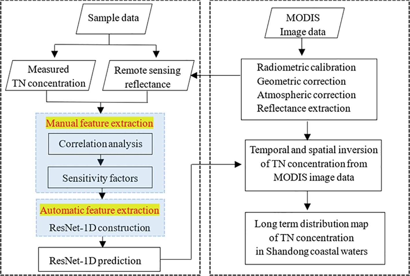
Figure 5 Technical roadmap.

4.1 Manual extraction and analysis of band features

There are only seven bands in MODIS data with spatial resolutions of 250 m and 500 m, which are too few to meet the inversion requirements. Therefore, it is necessary to integrate the original bands and construct new factors to make the features more diverse. The research shows that the band ratio can partially compensate for the influence of the atmosphere and effectively eliminate the interference of water surface roughness and environmental noise (Mohammad et al., 2016). Therefore, 21 factors are constructed through band ratio, combined with 7 original bands, and 28 characteristics are obtained. So, the correlations between 28 factors and TNC are analyzed, and the correlation coefficients are calculated, as shown in Figure 6.

Figure 6

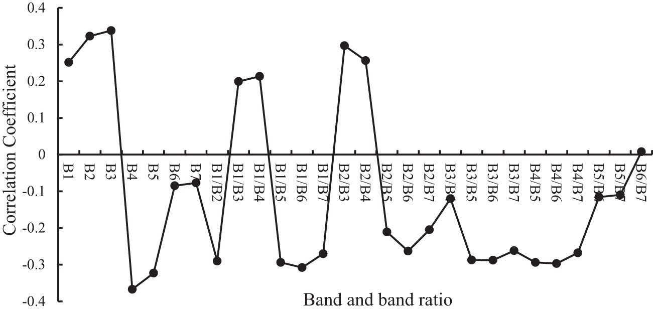
Figure 6 Correlation coefficient plot of band and band ratio.

Figure 6 shows that the correlation coefficients of all factors are between ± 0.4, indicating a weak linear correlation. The absolute values of the correlation coefficients of 5 elements are more significant than 0.3, ranging from high to low as B4, B3, B2, B5, and B1/B6. At the same time, the values of 13 factors are between 0.25 and 0.3, including B1/B2, B1/B5, B1/B7, B2/B3, B2/B4, B3/B5, B2/B6, B3/B5, B3/B6, B3/B7, B4/B5, B4/B6, and B4/B7, which are better than that of B6 and B7 band. In summary, with the help of band operation methods, the proportion bands with high correlation have been detected, enriching the feature information and providing a basis for selecting feature factors.

4.2 Construction of the ResNet-1D

With the gradual enhancement of layers in the deep learning network, the model parameters increase, so the required computational performance and the training difficulty of the model also augment accordingly. Considering that only a few of the 301 sample data exist, the network structure should not be too complex to avoid overfitting and challenging training. So, selecting a ResNet with fewer layers and appropriate feature factors is necessary. Therefore, the ResNet-18 is chosen in the paper, and 18 elements with a correlation greater than 0.25 are screened out as input factors of the one-dimensional residual network to inverse the TNC, which is recorded as the ResNet-1D model. The network structure and parameters are shown in Figure 7 and Table 6.

Figure 7

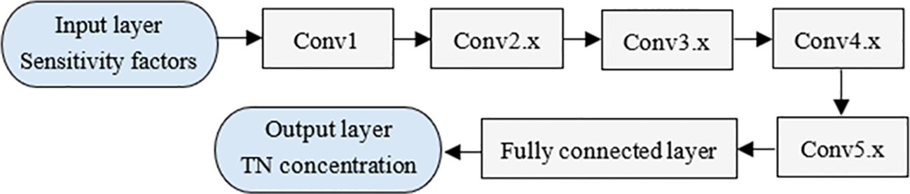
Figure 7 ResNet-1D structure diagram.

Table 6

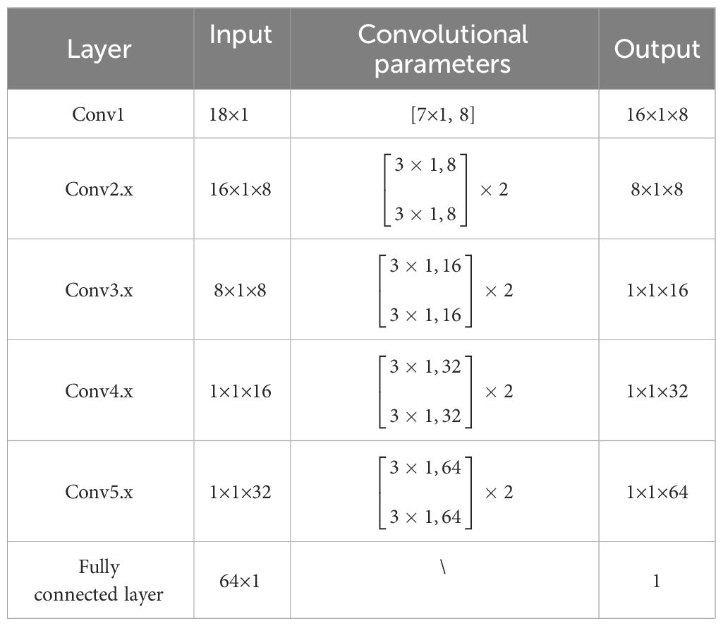
Table 6 Primary structure and parameters of the ResNet-1D.

The ResNet-1D model consists of an input layer, five convolutional layers, a fully connected layer, and an output layer. Among them, the input layer is composed of 18 nodes, the output layer is one node of the regression value., Conv1 involves only one convolution operation, Conv2.x~ Conv5.x contains two residual modules respectively; eight residual modules constitute four convolution layers. Because one residual module contains two convolution operations with the same depth, the ResNet-1D model contains 17 convolution operations, with convolution kernel sizes of 7, 3, 1, and step size of 1. The number of convolution kernels in each layer is 8, 8, 16, 32, and 64, respectively.

The input layer is one-dimensional data with 18 nodes, which is relatively small, so the pooling layers in the ResNet-18 have been removed. Meanwhile, after nine convolution operations in the former three convolutional layers, the number of nodes has been reduced to one, and the view field has expanded globally. Therefore, the eight convolution operations in convolutional layers 4 and 5 perform fully connected point convolutions.

After the convolution operations, all features are flattened into column vectors and inputted into the fully connected layer. The batch normalization operations are added before the activation function, which can weaken the gradient disappearance and improve the network’s generalization ability. Due to simplicity, the ReLU function is selected as the network’s activation function.

MRE is selected as the cost function. Considering the first and second moment estimation, the Adam algorithm is adopted to calculate the update step size. The initial learning rate is 9×10^-4, the learning rate attenuation factor is 0.6, the maximum train number is 200, and the batch size is 1. The early stop method is used to weaken the impact of overfitting.

The sample dataset is divided into train, validation, and test sets in a 6:2:2 ratio. When the train loss drops to 0.080, the mean absolute error of the train and validation set is about 0.215mg/L and 0.265mg/L, respectively, and the MRE of the test set is 39.64%. The R² of the train and test data is 0.84 and 0.72, respectively. The measured and inverted values of some points are shown in Figure 8.

Figure 8

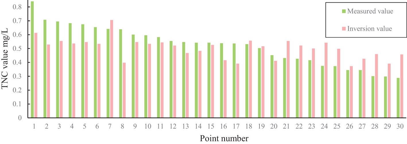
Figure 8 Results of inverted and measured values at test points.

Figure 8 shows that the measured values have a significant dispersion, with an average of 0.52 mg/L. By comparison, the inversion values have a small degree of distribution, with a mean of 0.50 mg/L. The absolute error increases gradually from the center of point 19 to both sides. Generally speaking, for measuring points with values greater than 0.5, the inversion value is smaller than the measured value. In contrast, the inversion value is more significant for measuring points with values less than 0.5.

The points of 8, 1, 2 in the high-value area and 21, 24, and 30 in the low-value area have relatively higher absolute error with values of 0.24, 0.22, 0.17, 0.16, 0.16, and 0.15, respectively. The corresponding MREs are 37.6%, 27.1%, 25.2%, 58.5%, 44.4%, and 52.6%. The points in the low-value area have significant relative errors due to the low-measured TNC values. It shows that the inversion ability of the ResNet-1D is weaker in the low value.

4.3 Preponderance analysis of the ResNet-1D

To compare with the ResNet-1D, the traditional BP neural network model (BP model), the particle swarm optimization BP neural network model (PSO-BP model), and the shallow convolutional network model (CNN model) are constructed. The datasets are divided into train and test sets in a 4:1 ratio in the first two models. The dataset partition of the CNN is the same as ResNet-1D.

The BP model is a fully connected neural network consisting of input, hidden, and output layers. To reduce parameters, the node number in the input and output layers is set to 5 and 1, respectively. The five factors with absolute correlation coefficients greater than 0.3 are input data, and the TNC values are output data. After repeated experiments, the number of hidden layer nodes is 8, the learning rate is 0.001, the expected error is 0.005, and the maximum number of training sessions is 3000. The Tansig and Purelin functions are used in the implicit and output layers, and the training function is Trainlm. The results show that the R² of the train and test data is 0.71 and 0.50, respectively. The latter is significantly lower than the former. The MREs are 45.64% and 62.86%. In conclusion, the BP model has low accuracy and poor generalization ability. Given this, the particle swarm algorithm is used to optimize the BP model, denoted as the PSO-BP model.

The PSO-BP model’s model structure remains unchanged, while the population size and evolution numbers are 10,100, and C1 and C2 are 2. The results show that the R² of the train and test data is 0.72 and 0.58, and the MRE is 46.99% and 49.25%. The PSO-BP model has the same effect as the BP model on the train set and performs better on the test.

The CNN model consists of four layers: one input layer, two convolution layers, and one output layer. The shape of the input layer is the same as the BP model. The parameters are optimized through a large number of experiments. The size and number of convolution kernels are 3 and 8; the sliding step size is 1, and the same convolution method is adopted. The results showed that the mean absolute error of the train set was about 0.270 mg/L when the train loss decreased to 0.135. The verification loss is about 0.195, and the MRE of the verification set and test set are about 0.350 mg/L and 51.66%, respectively, much lower than the BP model but slightly higher than the PSO-BP model. The R² is 0.76 and 0.65 for the two datasets.

From the BP to the CNN model, the number of network layers deepens from 3 to 4, and one full-connection operation in feature extraction is replaced by two convolution operations. As a result, the latter’s accuracy on the test and verification set is better than that of the former.

The precisions of the four models are listed in Table 7. In the train set, the MRE of the ResNet-1D model is the lowest, only 35.75%, while the MRE of the other three models is almost identical, about 46%. In the test set, the MREs of the four models are quite different. The ResNet-1D has the lowest MRE of 39.64%, and the BP model has the highest MRE of 62.86%. The PSO-BP and CNN models rank third and fourth, with 49.25% and 51.66%, respectively.

Table 7

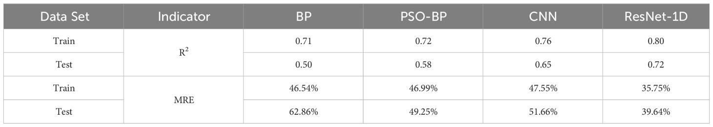
Table 7 Model comparison.

Whether in the train or test set, ResNet-1D has the lowest MRE and the highest R² of the four models, which is the optimal model with the highest accuracy and strongest generalization ability. The PSO-BP and CNN models are suboptimal, while the BP model is the worst. From the BP, CNN to ResNet-1D model, the number of feature factor nodes has increased, the network depth has deepened, and the model performance has improved.

5 Analysis

5.1 Analysis of spatiotemporal characteristics of TNC based on ResNet-1D

The ResNet-1D is used to invert the spatiotemporal characteristics of TNC in Shandong offshore. Since the model can only process one-dimensional data, pixel-by-pixel prediction is required for a two-dimensional image. After converting the image into one-dimensional data, the image pixels are inputted into the model in batches to achieve rapid processing. The corrosion and expansion operations are used to avoid fragmentation. Affected by the sampling time and the quality of satellite images, 34 spatiotemporal distribution maps of TNC were obtained in the Shandong coastal waters from 2008 to 2018, as shown in Figure 9. There are 6, 10, 10, and 8 periods in March, May, August, and October, respectively.

Figure 9

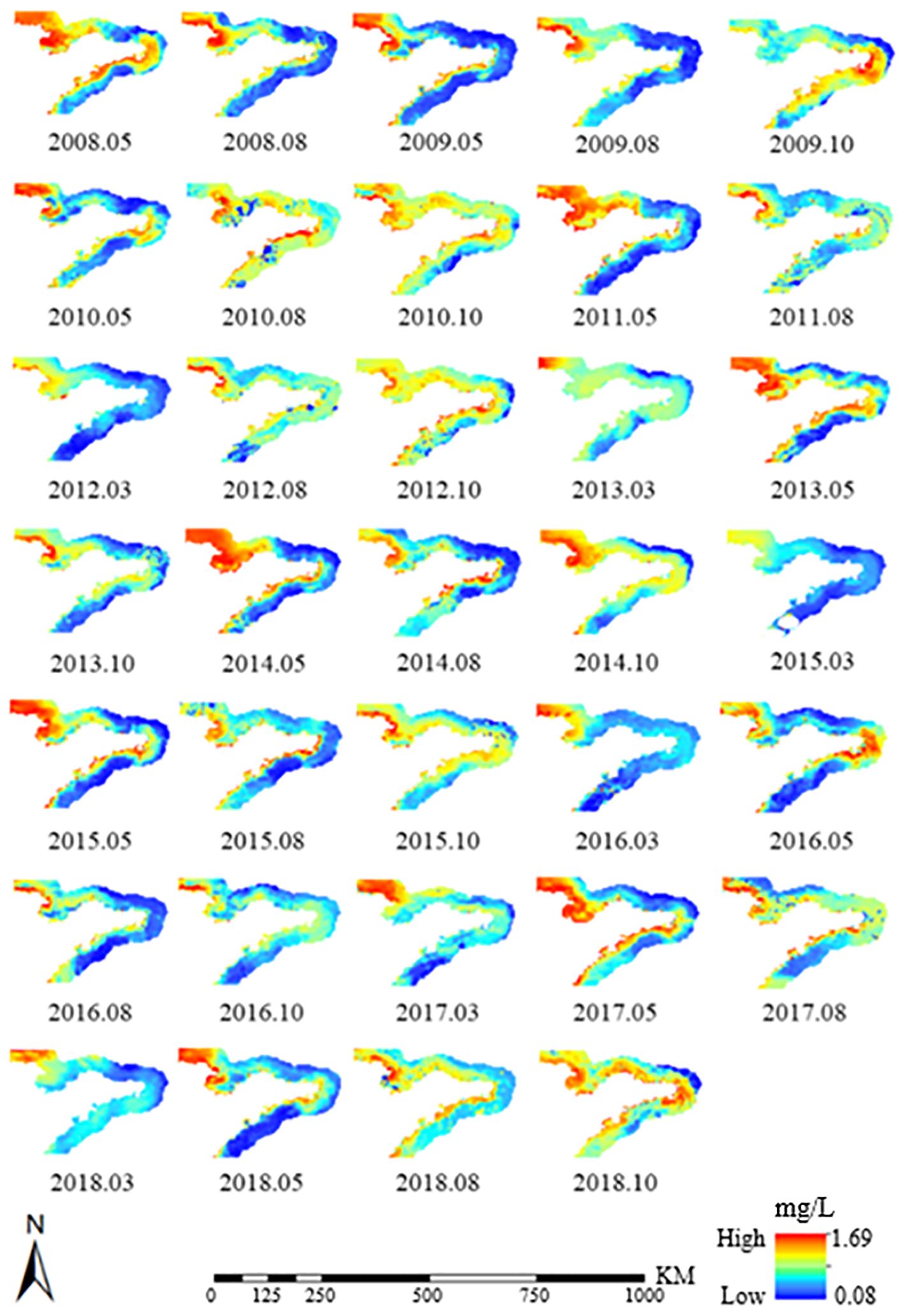
Figure 9 Distribution Map of TNC in Shandong Offshore from 2008 to 2018.

Regarding spatial distribution, the TNC in the coastal waters shows an overall trend of high inshore and low offshore, between 0.08 mg/L and 1.69 mg/L. The southern part of Bohai Bay and the northwestern part of Laizhou Bay are areas with high TNC, which occur more frequently. The frequency of the high-value area in the southeast of Weihai and the coastal waters of Qingdao is relatively low.

Based on Figure 9 and the measured data in Table 1, the seasonal variation chart of TNC in Shandong offshore was made, as shown in Figure 10. The picture shows that the overall concentration was lowest in March, medium in May and August, and highest in October, when the distribution of high-value areas expanded from land to sea compared with other months.

Figure 10

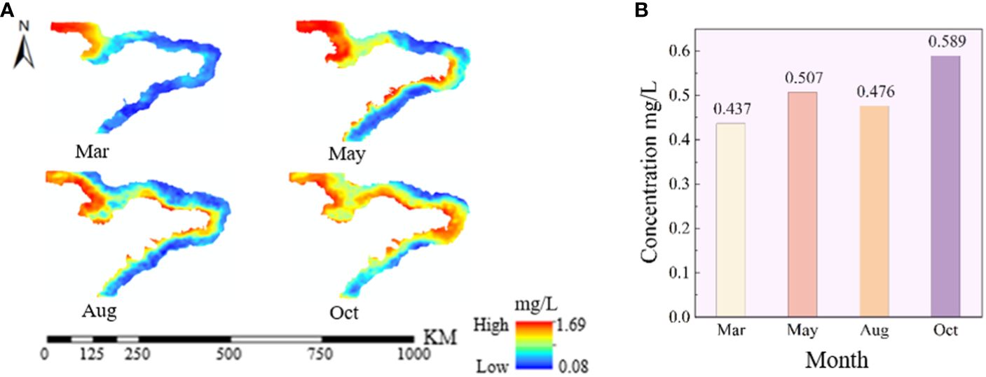
Figure 10 Seasonal variation of TNC in Shandong offshore. (A) Spatial distribution diagram of TNC inversion data. (B) Histogram of TNC measured data.

Regarding spatiotemporal distribution, the significant values of TNC in all seasons emerged in the southern area of Bohai Bay and the northwestern area of Laizhou Bay, which had the widest distribution and highest value in May, followed by October. The TNC was generally low in the coastal waters of the Peninsula in March. A banded high-value area appeared in the southern waters of the peninsula in May, which extended to the northern waters in August. In October, the high-value area further expanded from the above coastal waters to the far waters, among which the eastern waters of Weihai had the most apparent phenomenon.

The Shandong Peninsula is in the Jiaodong Economic Circle, which has muscular economic strength. It has many counties and more than 300 rivers flowing into the sea. The total area exceeds 50,000 km², accounting for about 30% of Shandong Province, and the entire population surpasses 30 million. Therefore, many high-intensity human and industrial activities, as well as the eutrophic water bodies injected into the coastal waters, will strongly affect the quality of the coastal waters. The tides cause water exchange, resulting in solid turbulence of the shallow coastal waters, impacting coastal water quality. Compared with coastal water, offshore water is less affected by human activities and surface runoff, has a relatively stable marine environment, and has a lower TNC.

Many rivers that carry eutrophic fresh water, such as the Yellow River and the Weihe River, flow into the sea at Laizhou Bay and Bohai Bay. As a result, the TNC in the above two regions is higher than in other areas, especially in May and August, when precipitation is abundant.

The Shandong Peninsula has a warm, temperate, humid monsoon climate. The annual precipitation is 650 to 850 mm. The summer precipitation is abundant, accounting for about 60% of the annual precipitation, while the spring and autumn precipitation is less. The annual humidity changes are severe, with dry and windy spring, high humidity in summer, and monsoons prevalent in winter. In addition, due to the influence of the physical properties of land and sea, the environment in some areas is complex and variable. The above factors jointly affect the change in the water environment in Shandong’s coastal waters.

In summary, the overall change in TNC is closely related to human activities, industrial and agricultural production, climate, precipitation, surface runoff into the sea, and tides.

5.2 Analysis of interannual variation characteristics of TNC based on measured data

The image amounts of each year are inconsistent, and the distribution of TNC in each month is quite different, so the interannual change trend of TNC based on Figure 9 is not apparent. In this paper, measured data were used to carry out this study, and the average chart of TNC for each year is shown in Figure 11, which visually shows the interannual variation of TNC in the study area from 2008 to 2018.

Figure 11

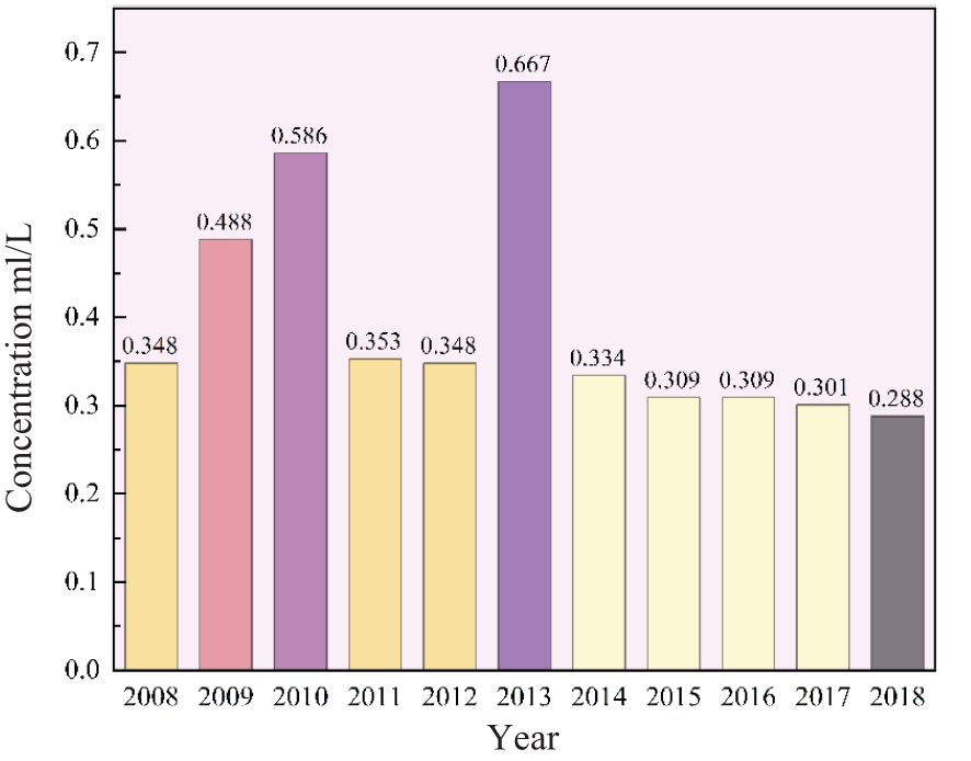
Figure 11 Annual mean value histogram of TNC measured data.

Figure 11 shows that the interannual variation of TNC can be clearly divided into two periods: the variation period of the broken line from 2008 to 2014 and the constant period of the approximate straight line from 2015 to 2018. In the previous period, the TNC had a distribution trend of two liters and two drops. In the later period, it had a stable and slightly reduced distribution characteristic.

Shandong province has implemented a drainage basin pollution control system. Taking small drainage basins as control units, pollution prevention, cyclic utilization, and ecological protection were implemented, and the aquatic environment quality has been significantly improved. By the end of 2010, fish growth had recovered in 58 heavily polluted rivers, and the water quality indexes of major rivers basically met the requirements of Case V Waters (Zhou and Ji, 2016). The regulation and improvement of rivers entering the sea were completed. In 2016, China put forward the Blue Bay Action. The goal is to improve the marine environment quality and enhance the ecological functions of the coast, marine, and island.

Therefore, the TNC in the coastal waters of Shandong has been less than 0.35 since 2011 and slightly decreased because of measures such as controlling the discharge of land pollutants into the sea, reducing ecological damage, implementing ecological protection and restoration, and comprehensive prevention and ecological environment control of land, shore, and marine. The environmental treatment of coastal waters in Shandong Province has been successful. Nevertheless, the high value in 2013 may be a singular value.

6 Discussion

(1) The spectral data is commonly used in water quality parameter inversion models. However, the number of bands is limited sometimes, and some correlate poorly with water quality parameters. Therefore, band features can be manually extracted by band ratio to extend the sensitive factors, which can eliminate the influence of the atmosphere and environment. Pearson analysis calculates the correlation between each factor and TNC. Although this method cannot describe nonlinear relationships, the research has shown that the Pearson correlation coefficients of some ratio factors are more significant than those of single bands. The factors with large correlation coefficients can be used as input factors of the inversion model, thereby improving the model’s accuracy.

(2) There is a type II water body in the coastal area whose optical properties are much more complex than those of ocean water. The absorption and scattering regions of chlorophyll, suspended sediment, and dissolved organic matter overlap in the spectrum. The relationship between TNC and remote sensing reflectance is non-linear and complex. In this study, the correlations between index factors and TNC are less than 0.4, which may indicate a significant nonlinear mapping relationship between various factors and TNC from the other side. Therefore, the selection of a nonlinear inversion model is crucial.

(3) Because the nonlinear model has the double ability of both linear and nonlinear fitting, five factors with high correlation coefficients can be selected as the input of BP, PSO-BP, and CNN models, and 18 factors can be chosen as the input of the ResNet-1D model. The calculation result shows that the accuracy of the first three models on the train set is almost identical. On the test set, the precision of the PSO-BP and CNN models is roughly the same, but it is significantly higher than that of the BP model. That is, the CNN and BP models have the same input, and the network structure of the former is more than that of the latter; the accuracy is higher. The ResNet-1D model has the most input factors and the deepest layers. With the increase of indicator factors and the depth of the model, the automatic feature extraction ability is further enhanced, and the performance is the best on both the test and train set, making it the optimal model in this article.

(4) Many composite variables are used in the ResNet-1D model, derived from specific operations between different bands, demonstrating that the estimation of TNC is affected by many complex factors. Therefore, machine learning models such as BP, PSO-BP, and CNN are challenging to match the accuracy of the ResNet-1D due to the small number and the single type of variables. Therefore, the remote sensing inversion of TNC requires the participation of multiple and polytype variables.

(5) The ResNet-1D model has added 13 indicator factors and is deepened to 18 layers compared with the BP, PSO-BP, and CNN models. Although the Pearson coefficients of the factors are low, the model improves the inversion accuracy and generalization performance by increasing network depth to automatically extract deep features, back-propagation to update weights, and setting identity mapping to make the model easy to optimize. Therefore, the MRE on both datasets is decreased by at least 10%, and the nonlinear relationship between the two data types is fully fitted in the ResNet-1D model.

(6) The quantitative research of water quality parameters mainly focuses on estimating light-sensitive variables, such as total suspended solids, chlorophyll-a, and turbidity. In contrast, some non-photosensitive indicators, such as TN, pH, dissolved phosphorus, etc., have no significant spectral response in the visible and near-infrared regions, and the inversion accuracy is significantly lower than the above light-sensitive parameters (Mohammad et al., 2016; Liu et al., 2020). Although the ResNet-1D is the optimal inversion model constructed in this paper, its R² on the two data sets is 0.8 and 0.72, which are reasonable. However, the MRE is only 35.7% and 39.6%, which are large, and there is still a significant gap in the practical application. However, theoretical approaches such as increasing the number of input factors, deepening network layers, extracting deep features, and using nonlinear inversion models are discussed in this article in the case of a few satellite band data and low correlation coefficients of constructed indicators. The result shows that the MRE of the ResNet-1D is reduced by 23% compared to the traditional BP model and nearly 10% compared to the suboptimal PSO-BP model. This has a specific guiding significance for the inversion of non-photosensitive substances in the water body. Although the inversion accuracy of the ResNet-1D model is only 60%, the TN concentration map inverted by the model can reflect the spatiotemporal trend and has a certain reference value.

(7) Through a series of convolution operations, the deep residual network transforms the features of samples in the original space into the new feature space and automatically obtains the hierarchical feature representation. The training difficulty of the network is reduced by adding residual learning units to the convolutional layer, and the network automatically updates the weights through backpropagation in the residual network (He et al., 2016). Because of these merits, it is widely used in data analysis. Among them, in one-dimensional spectral data analysis, Lu employed the measured hyperspectral data as the data source and the one-dimensional residual network as the inversion model to obtain the haze monitoring results in Suzhou City (Lu et al., 2017). In 2D image data processing, Li proposed a multi-scale edge detection algorithm for medical ultrasonic images based on a two-dimensional deep ResNet (Li et al., 2021); Wang and Duan had combined a two-dimensional deep ResNet with wavelet transform for image super-resolution (Duan et al., 2019; Wang et al., 2022). In this study, ResNet-1D was applied to the inversion of TNC in the coastal waters of Shandong. Compared with the traditional model, it showed higher inversion accuracy due to the automatic extraction of deep features, automatic updating of weights, and automated determination of optimal thresholds. This study has provided a scientific method that extends a limited set of field observation data to areas or times where field data are not available. However, the applicability of this method in other sea areas needs to be further verified.

7 Conclusion

The TN inversion in Shandong coastal waters is set as the research object. The measured TNC and MODIS remote sensing image’s reflectance are data sources. The two-step feature extraction is adopted as a means, and the ResNet-1D is constructed as an inversion model. The spatial and temporal distribution characteristics of TNC from 2008 to 2018 are explored. The main conclusions are as follows:

(1) The ResNet-1D can automatically extract the deep features based on manually extracted features and improve the inversion model’s accuracy. Based on the operation between bands, the shallow features are extended. The correlation analysis between all the shallow factors and TNC is carried out. Five factors with significant correlation coefficients are screened out as the input of the BP, PSO-BP, and CNN models, and 18 factors are used as the input of the ResNet-1D to extract the deep features. The results show that the ResNet-1D has the highest accuracy, indicating that the deep model automatically extracts deep features and realizes complex nonlinear mapping with increased input factors and model layers.

(2) The ResNet-1D can inverse the spatiotemporal distribution characteristics in the coastal waters of Shandong Province from 2008 to 2018. The research indicates that the TNC in the region is between 0.08 mg/L and 1.69 mg/L. Regarding spatial distribution, the near-shore concentration is higher than the far-shore. The frequency of high-value areas on the peninsula’s north coast is higher than on the southeast. Regarding time distribution, the overall concentration is low in spring, middle in summer, and high in autumn. The distribution range of high-value areas is expanded in autumn compared with other seasons. In terms of interannual variation, TNC had a trend of two increases and two decreases in the first seven years and characteristic of stable and slightly reduced distribution in the last four years. Although the inversion accuracy of the ResNet-1D model is only 60%, the TNC map inverted by the model can reflect the spatiotemporal trend and has a certain reference value.

The inversion of TNC is still in the exploratory stage, limited by the number of sampling points, satellite image resolution, regional conditions, and inversion models. In the future, expanding the sampling point, increasing the spectral index factor, fusing images of different resolutions, extending the spatiotemporal monitoring range, and improving inversion models will be necessary.

Data availability statement

The raw data supporting the conclusions of this article will be made available by the authors, without undue reservation.

Author contributions

HZ: Writing – review & editing, Data curation, Investigation. YW: Conceptualization, Visualization, Writing – original draft. HH: Methodology, Resources, Writing – review & editing. JW: Investigation, Methodology, Resources, Validation. SL: Funding acquisition, Project administration, Resources, Supervision, Writing – review & editing. MX: Project administration, Validation, Visualization, Writing – original draft. JC: Formal analysis, Investigation, Methodology, Resources, Supervision, Writing – review & editing. MY: Writing – review & editing.

Funding

The author(s) declare financial support was received for the research, authorship, and/or publication of this article. This research was funded by the National Natural Science Foundation of China, grant numbers U1906217 and 62071491, and the Fundamental Research Funds for the Central Universities, grant numbers 22CX01004A-4 and 22CX01004A-5.

Acknowledgments

The authors would like to take this opportunity to thank the editors and the reviewers for their detailed comments and suggestions.

Conflict of interest

Author YW were employed by the company Wei chai Power Co., Ltd.

The remaining authors declare that the research was conducted in the absence of any commercial or financial relationships that could be construed as a potential conflict of interest.

Publisher’s note

All claims expressed in this article are solely those of the authors and do not necessarily represent those of their affiliated organizations, or those of the publisher, the editors and the reviewers. Any product that may be evaluated in this article, or claim that may be made by its manufacturer, is not guaranteed or endorsed by the publisher.

References

Amiri B. J., Nakane K. (2009). Comparative prediction of stream water total nitrogen from land cover using artificial neural network and multiple linear regression approaches. Polish J. Environ. Stud. 18, 151–160.

Google Scholar

Cao Z. G., Ma R. H., Duan H. T. (2020). A machine learning approach to estimate chlorophyll-a from Landsat-8 measurements in inland lakes. Remote Sens. Environ. 248, 111974. doi: 10.1016/j.rse.2020.111974

CrossRef Full Text | Google Scholar

Cao Z. G., Ma R. H., Melack J. M. (2022). Landsat observations of chlorophyll-a variations in Lake Taihu from 1984 to 2019. Int. J. Appl. Earth Observation Geoinf. 106, 102642. doi: 10.1016/j.jag.2021.102642

CrossRef Full Text | Google Scholar

Carpenter D. J., Carpenter S. M. (1983). Modeling inland water using Landsat data. Remote Sens. Environ. 13, 345–352. doi: 10.1016/0034-4257(83)90035-4

CrossRef Full Text | Google Scholar

Chen Q. (2006). Effects of nitrogen and phosphorus on the occurrence of water blooms. Bull. Biol. 41, 12–14.

Google Scholar

Chen S. L., Hu C. M., Brian B. B. (2019). A machine learning approach to estimate surface ocean pCO2 from satellite measurements. Remote Sens. Environ. 228, 203–226. doi: 10.1016/j.rse.2019.04.019

CrossRef Full Text | Google Scholar

Conley D. J., Paerl H. W., Howarth R. W. (2009). Controlling eutrophication: Nitrogen and phosphorus. Science 323, 1014–1015. doi: 10.1126/science.1167755

PubMed Abstract | CrossRef Full Text | Google Scholar

Dong W., Yang Y., Qu J., Xiao S., Li Y. (2023). Local information enhanced graph-transformer for hyperspectral image change detection with limited training samples. IEEE Trans. Geosci. Remote Sens. 61, 1–14. doi: 10.1109/TGRS.2023.3269892

CrossRef Full Text | Google Scholar

Duan L. J., Wu C. L., En Q. (2019). Deep residual network in wavelet domain for image super-resolution. J. Softw. 30, 941–953. doi: 10.13328/j.cnki.jos.005663

CrossRef Full Text | Google Scholar

Fang X. R., Wen Z. F., Chen J. L. (2019). Remote sensing estimation of suspended sediment concentration based on random forest regression model. J. Remote Sens. 23, 756–772. doi: 10.11834/jrs.20197498

CrossRef Full Text | Google Scholar

Guildford S. J., Hecky R. E. (2000). Total nitrogen, total phosphorus, and nutrient limitation in lakes and oceans: Is there a common relationship? Limnol. Oceanogr. 45, 1213–1223. doi: 10.4319/lo.2000.45.6.1213

CrossRef Full Text | Google Scholar

Han B. H., Zhao Q. C., Chang R. (2023). Chlorophyll-a concentration inversion model: Stacked auto-encoder particle swarm optimization BP neural network. J. Geo-inf. Sci. 25, 1882–1893. doi: 10.12082/dqxxkx.2023.230144

CrossRef Full Text | Google Scholar

Harvey E. T., Kratzer S., Philison P. (2015). Satellite-based water quality monitoring for improved spatial and temporal retrieval of chlorophyll-a in coastal waters. Remote Sens. Environ.: Interdiscip. J. 158, 417–430. doi: 10.1016/j.rse.2014.11.017

CrossRef Full Text | Google Scholar

He K. M., Zhang X. Y., Ren S. Q. (2016). “Deep residual learning for image recognition,” in IEEE Computer Society Conference on computer Vision and Pattern Recognition, Las Vegas, NY, USA. 770–778.

Google Scholar

Le Q. V. (2013). “Building high-level features using large-scale unsupervised learning,” in EEE International Conference on Acoustics, Speech, and Signal Processing, Vancouver, BC, Canada, 8595–8598.

Google Scholar

Lecun Y., Bengio Y., Hinton G. (2015). Deep learning. Nature 521, 14539. doi: 10.1038/nature14539

CrossRef Full Text | Google Scholar

Li H. (2018). Deep learning for natural language processing: advantages and challenges. Natl. Sci. Rev. 5, 24–26. doi: 10.1093/nsr/nwx110

CrossRef Full Text | Google Scholar

Li E. (2020). Research on inversion method of Nitrogen and Phosphorus content based on UAV hyperspectral remote sensing (Dalian: Dalian Maritime university).

Google Scholar

Li X. F., Li D., Wang Y. W. (2021). Multi-scale edge detection algorithm for medical ultrasonic image based on deep residual network. J. Jilin Univ. (Sci. Ed.) 59, 900–908. doi: 10.13413/j.cnki.jdxblxb.2020169

CrossRef Full Text | Google Scholar

Liu C. J., Zhang F., Ge X. Y. (2020). Measurement of total nitrogen concentration in surface water using hyperspectral band observation method. Water 12, 1842. doi: 10.3390/w12071842

CrossRef Full Text | Google Scholar

Liu J. M., Zhang Y. J., Yuan D. (2015). Empirical estimation of total nitrogen and phosphorus concentration of urban water bodies in China using high-resolution IKONOS multispectral imagery. Water 7, 6551–6573. doi: 10.3390/w7116551

CrossRef Full Text | Google Scholar

Lu Y. S., Li Y. X., Liu B. (2017). Hyperspectral data haze monitoring based on deep residual network. Acta Optica Sin. 37, 1128001. doi: 10.3788/AOS201737.1128001

CrossRef Full Text | Google Scholar

Maier P. M., Sina K., Stefan H. (2021). Deep learning with WASI simulation data for estimating Chlorophyll a concentration of inland water bodies. Remote Sens. 2021, 718. doi: 10.3390/rs13040718

CrossRef Full Text | Google Scholar

Marmanis D., Datcu M., Esch T. (2016). Deep learning earth observation classification using image net pre-trained networks. IEEE Geosci. Remote Sens. Lett. 13, 105–109. doi: 10.1109/LGRS.2015.2499239

CrossRef Full Text | Google Scholar

Mohammad G., Assefa M., Lakshmi R. (2016). A comprehensive review on water quality parameters estimation using remote sensing techniques. Sensors 16, 1298–1340. doi: 10.3390/s16081298

PubMed Abstract | CrossRef Full Text | Google Scholar

Muhammad Y., Sheng H., Fan H. (2020). Automatic coastline extraction and changes analysis using remote sensing and GIS technology. IEEE Access 8, 180156–180170. doi: 10.1109/ACCESS.2020.3027881

CrossRef Full Text | Google Scholar

Muhammad Y., Wan J. H., Liu S. W. (2022). Coupling of deep learning and remote sensing: a comprehensive systematic literature review. Int. J. Remote Sens. 44, 157–193. doi: 10.1080/01431161.2022.2161856

CrossRef Full Text | Google Scholar

Pahlevan N., Smith B., Schalles J. (2020). Seamless retrievals of chlorophyll-a from Sentinel-2 (MSI) and Sentinel-3 (OLCI) in inland and coastal waters: A machine-learning approach. Remote Sens. Environ. 240, 111604. doi: 10.1016/j.rse.2019.111604

CrossRef Full Text | Google Scholar

Pu F. L., Ding C. J., Chao Z. Y. (2019). Water-quality classification of inland lakes using Landsat 8 images by convolutional neural networks. Remote Sens. 11, 1674. doi: 10.3390/rs11141674

CrossRef Full Text | Google Scholar

Pyo J. C., Ligaray M., Kwon Y. S. (2018). High-spatial resolution monitoring of phycocyanin and chlorophyll-a using airborne hyperspectral imagery. Remote Sens. 10, 1180. doi: 10.3390/rs10081180

CrossRef Full Text | Google Scholar

Qin B. Q., Yang L. Y., Chen F. Z. (2006). Mechanism and control technology of lake eutrophication and its application. Chin. Sci. Bulletin 51, 1857–1866. doi: 10.1007/s11434-006-2096-y

CrossRef Full Text | Google Scholar

Reilly J. E., Werdell P. J. (2019). Chlorophyll algorithms for ocean color sensors-OC4, OC5 & OC6. Remote Sens. Environ. 229, 32–47. doi: 10.1016/j.rse.2019.04.021

PubMed Abstract | CrossRef Full Text | Google Scholar

Riese F. M., Keller S. (2019). “Soil texture classification with 1D convolutional neural networks based on hyperspectral data,” in ISPRS Annals of the potogrammetry, Remote Sensing and Spatial Information Sciences, Enschede, Netherlands. 615–621.

Google Scholar

Sagan V., Perterson K. T., Maimaitijiang M. S. (2020). Monitoring inland water quality using remote sensing: potential and limitations of spectral indices, bio-optical simulations, machine learning, and cloud computing. Earth-Sci. Rev. 205, 103187. doi: 10.1016/j.earscirev.2020.103187

CrossRef Full Text | Google Scholar

Serwan M. J. (1993). Detecting water quality parameters in the Norfolk Broads, U.K., using Landsat imagery. Int. J. Remote Sens. 14, 1247–1267. doi: 10.1080/01431169308953955

CrossRef Full Text | Google Scholar

Shen M., Duan H. T., Cao Z. G. (2020). Sentinel-3 OLCI observations of water clarity in large lakes in eastern China: Implications for SDG evaluation. Remote Sens. Environ. 247, 111950. doi: 10.1016/j.rse.2020.111950

CrossRef Full Text | Google Scholar

Sheng H., Chi H. X., Xu M. M. (2021). Inland water chemical oxygen demand estimation based on improved SVR for hyperspectral data. Spectrosc. Spectral Analysis 41, 3565–3571. doi: 10.3964/j.issn.1000-0593(2021)11-3565-07

CrossRef Full Text | Google Scholar

Smith V. H., Tilman G. D., Nekola J. C. (1999). Eutrophication: impacts of excess nutrient inputs on freshwater, marine, and terrestrial ecosystem. Environ. Pollution 100, 179–196. doi: 10.1016/S0269-7491(99)00091-3

CrossRef Full Text | Google Scholar

Song K., Li L., Li S. (2012). Hyperspectral remote sensing of total phosphorus (TP) in three central Indiana water supply reservoirs. Water Air Soil Pollution 223, 1481–1502. doi: 10.1007/s11270-011-0959-6

CrossRef Full Text | Google Scholar

Soomets T., Uudeberg K., Jakovels D. (2020). Validation and comparison of water quality products in Baltic Lakes using sentinel-2 MSI and sentinel-3 OLCI Data. Sensors 20, 742. doi: 10.3390/s20030742

PubMed Abstract | CrossRef Full Text | Google Scholar

Sun X. T., Fu Y., Han C. X. (2023). An inversion method for chlorophyll-a concentration in the global ocean through convolutional neural networks. Spectrosc. Spectral Analysis 43, 608–613. doi: 10.3964/j.issn.1000-0593(2023)02-0608-06

CrossRef Full Text | Google Scholar

Sun D. Y., Qiu Z. F., Li Y. M. (2014). Detection of total phosphorus concentrations of turbid inland waters using a remote sensing method. Water Air Soil Pollution 225, 1–17. doi: 10.1007/s11270-014-1953-6

CrossRef Full Text | Google Scholar

Uudeberg K., Aavaste A., Kõks K. (2020). Optical water type guided approach to estimate optical water quality parameters. Remote Sens. 12, 931–965. doi: 10.3390/rs12060931

CrossRef Full Text | Google Scholar

Wagle N., Acharya T. D., Lee D. H. (2020). A comprehensive review on application of machine learning algorithms for water quality parameter estimation using remote sensing data. Sens. Mater. 32, 3879–3892. doi: 10.18494/SAM.2020.2953

CrossRef Full Text | Google Scholar

Wang X. H., Zhao X. Y., Wang X. Y. (2022). Single image super-resolution reconstruction using deep residual networks with non-decimated wavelet edge learning. Acta Electronica Sin. 50, 1753–1765. doi: 10.12263/DZXB.20210854

CrossRef Full Text | Google Scholar

Wen Z., Wang Q., Ma Y. (2024). Remote estimates of suspended particulate matter in global lakes using machine learning models. Int. Soil Water Conserv. Res. 12, 200–216. doi: 10.1016/j.iswcr.2023.07.002

CrossRef Full Text | Google Scholar

Yin L., Wang L., Li T. (2023a). U-Net-LSTM: time series-enhanced lake boundary prediction model. Land 12, 1859. doi: 10.3390/land12101859

CrossRef Full Text | Google Scholar

Yin L., Wang L., Li T. (2023b). U-Net-STN: A novel end-to-end lake boundary prediction model. Land 12, 1602. doi: 10.3390/land12081602

CrossRef Full Text | Google Scholar

Yu B. W. (2019). Global Chlorophyll-a concentration estimation from VIIRS using deep learning methods (Bei Jing: China University of Geoscience (Bei Jing).

Google Scholar

Yu B. W., Xu L. L., Peng J. H. (2020). Global chlorophyll-a concentration estimation from moderate resolution imaging spectroradiometer using convolutional neural networks. J. Appl. Remote Sens. 14, 34520. doi: 10.1117/1.JRS.14.034520

CrossRef Full Text | Google Scholar

Yu X., Yi H. P., Liu X. Y. (2016). Remote-sensing estimation of dissolved inorganic nitrogen concentration in the Bohai Sea using band combinations derived from MODIS data. Int. J. Remote Sens. 37, 327–340. doi: 10.1080/01431161.2015.1125555

CrossRef Full Text | Google Scholar

Zhang B., Li J. S., Shen Q. (2021). Recent research progress on long-time series and large-scale optical remote sensing of inland water. Natl. Remote Sens. Bulletin 25, 37–52. doi: 10.11834/jrs.20210570

CrossRef Full Text | Google Scholar

Zhao W. Z., Du S. H. (2016). Spectral-spatial feature extraction for hyperspectral image classification: A dimension reduction and deep learning approach. IEEE Transaction Geosci. Remote Sens. 54, 4544–4554. doi: 10.1109/TGRS.2016.2543748

CrossRef Full Text | Google Scholar

Zhou Y. L., Ji Y. D. (2016). Shan Dong is striving to upgrade water pollution prevention and control. China Environ. News 8, 1.

Google Scholar

Zhu Y., Zhu L., Li J. G. (2017). The study of inversion of chlorophyll a in Taihu based on GF-1 WFV image and BP neural network. Acta Scientiae Circumstantiae 37, 130–137. doi: 10.13671/j.hjkxxb.2016.0275

CrossRef Full Text | Google Scholar