 Chuang Rui
 Zhengya Sun
 Wensheng Zhang1
 An-An Liu
94% of researchers rate our articles as excellent or good
Learn more about the work of our research integrity team to safeguard the quality of each article we publish.
Find out more
ORIGINAL RESEARCH article
Front. Mar. Sci., 12 February 2024
Sec. Ocean Observation
Volume 11 - 2024 | https://doi.org/10.3389/fmars.2024.1334210
This article is part of the Research TopicDeep Learning for Marine Science, volume IIView all 27 articles
El Niño-Southern Oscillation (ENSO), a cyclic climate phenomenon spanning interannual and decadal timescales, exerts substantial impacts on the global weather patterns and ecosystems. Recently, deep learning has brought considerable advances in the accurate prediction of ENSO occurrence. However, the current models are insufficient to characterize the evolutionary behavior of the ENSO, particularly lacking comprehensive modeling of local-range and longrange spatiotemporal interdependencies, and the incorporation of calendar monthly and seasonal properties. To make up this gap, we propose a Two-Stage SpatioTemporal (TSST) autoregressive model that couples the meteorological factor prediction with ENSO indicator prediction. The first stage predicts the meteorological time series by leveraging self-attention ConvLSTM network which captures both the local and the global spatial-temporal dependencies. The temporal embeddings of calendar months and seasonal information are further incorporated to preserves repeatedly-occurring-yet-hidden patterns in meteorological series. The second stage uses multiple layers to extract higher level of features from predicted meteorological factors progressively to generate ENSO indicators. The results demonstrate that our model outperforms the state-of-the-art ENSO prediction models, effectively predicting ENSO up to 24 months and mitigating the spring predictability barrier.
ENSO is currently the world’s largest coupled ocean–atmosphere model, which occurs in the equatorial central and eastern Pacific Wang and Fiedler (2006). It leads to cyclic changes in Pacific sea surface temperatures, impacting global climate and ecosystems, including floods Dilley and Heyman (1995), droughts Lv et al. (2022), tropical cyclones Lin et al. (2020a) and coral reefs Manzello et al. (2014). Therefore, accurately predicting ENSO is crucial for promoting environmental, economic, and social sustainability Fiedler (2002); Adams et al. (1999); Tang et al. (2018).
ENSO prediction mainly relies on spatiotemporal data of meteorological factors, like Sea Surface Temperature (SST) and Heat Content (HC) McPhaden (2003); Cheng et al. (2019), which possess complex spatial and temporal connections. On the one hand, closer locations tend to exhibit stronger connections, adhering to the First Law of Geography Tobler (2004), but due to factors like global atmospheric circulation Alexander et al. (2002), large-scale meteorological fluctuations McPhaden et al. (2006), monsoonl Kumar et al. (1999) and ocean currents Cai et al. (2015), long-distance connections can also exist, known as spatial teleconnections Rajagopalan et al. (2000). On the other hand, shorter time intervals result in stronger connections, but periodicity in meteorological factors leads to significant connections even in longer intervals Jin and Kirtman (2010).
In addition, influenced by factors like solar radiation and Earth’s rotation Chapanov et al. (2017), ENSOrelated meteorological sequences often display pronounced calendar month and seasonal characteristics, particularly in ENSO development, prediction accuracy, and precursor signals Ham et al. (2021). Firstly, an ENSO event typically begins to develop during boreal spring, rapidly grows during summer and autumn, and reaches its maximum amplitude in winter. These different phases of ENSO events can be distinguished based on calendar months and seasons, showing a seasonal phase-locking pattern Dommenget and Yu (2016). This can be explained as low-order chaotic behavior driven by the seasonal cycle Tziperman et al. (1994); Tziperman et al., 1995). Some studies also reveal that the seasonally modulated termination process of big El Niño events is related to a combination mode, which originates from the atmospheric nonlinear interaction between ENSO and the Pacific warm pool annual cycle Stuecker et al. (2013); Ren et al. (2016). Secondly, the predictability of ENSO events varies across months and seasons. For instance, during boreal spring when ENSO is in its formation phase, the ENSO signal is relatively weak and susceptible to interference from other signals, leading to higher forecasting challenges in spring, known as the spring prediction barrier Lopez and Kirtman (2014). Thirdly, ENSO precursors also exhibit seasonality. For example, the Indian Ocean Dipole (IOD) reaches its peak strength in autumn but is negligible in other seasons Lestari and Koh (2016).
Based on the varying utilization of temporal and spacial characteristics, current deep learning-based models for ENSO prediction can be categorized into three types. The first type solely relies on temporal features. Broni-Bedaiko et al.Broni-Bedaiko et al. (2019) and Yan et al.Yan et al. (2020) utilizing LSTM and TCN networks, respectively, to capture the temporal evolution of meteorological factors. The second type exclusively leverages spatial features. Ham et al.Ham et al. (2019) employ CNN networks to capture space interdependencies among meteorological factors, achieving effective forecasting up to 16 lead months. However, due to the local connectivity and network depth limitations of CNNs, their efficiency in modeling long-range spatial relationships is diminished. In contrast, F. Ye et al. Ye et al. (2021a) utilize Transformer networks to enhance long-range spatial modeling, resulting in an improvement in predictive performance. The third type simultaneously utilizes both spatial and temporal features. Zhao et al. Zhao et al. (2023) employ a combination of 1D convolutions in the temporal dimension and 2D convolutions in the spatial dimension to simultaneously capture spatiotemporal features and directly predict future ENSO indicators. Wang et al. Wang et al. (2023) utilized a TCN branch to extract temporal features and a 2D CNN branch to extract spatial features. Geng and Wang Geng and Wang (2021) utilize a Casual-LSTM network to extract spatiotemporal features and forecast future meteorological factors, however, they fall short in modeling long-range spatiotemporal dependencies. On the other hand, Zhou and Zhang Zhou and Zhang (2023) utilize a spatiotemporal Transformer network to extract features and predict future meteorological factors. Although they can capture long-range spatiotemporal dependencies, the Transformer network treats temporal and spatial inputs equally, lacking an inductive bias for modeling close-range spatiotemporal dependencies efficiently. Furthermore, all three methods lack modeling of calendar month and seasonal characteristics.
To comprehensively model the temporal and spatial connections, as well as account for calendar monthseasonal characteristics of meteorological factors, we propose a Two-Stage SpatioTemporal (TSST) autoregressive method for ENSO forecasting. In Stage 1, we employ a spatiotemporal sequence prediction model that combines the Self-Attention ConvLSTM (SAConvLSTM) Lin et al. (2020b) module with a temporal embedding module. It receives the spatiotemporal sequences of Sea Surface Temperature Anomalies (SSTA, indicating deviations from the long-term historical average of sea surface temperature), and Heat Content Anomalies (HCA, indicating deviations from the long-term historical average of ocean heat content), observed over the preceding 12 months. The model then predicts the sequences of these anomalies for the next 26 months. The SAConvLSTM module is utilized to simultaneously model both close-range and long-range spatiotemporal dependencies. The temporal embedding module encodes calendar month and seasonal information using two methods: periodic functions and learnable parameters. The periodic functions transform calendar month and seasonal information into fixed representations, providing stable temporal priors. The learnable parameters approach encodes calendar month and seasonal information into adaptable representations, learning distinct features for different calendar months and seasons from the data, capturing finer variations in the data. In Stage 2, a CNN-based mapping model is employed to refine the predictions from Stage 1 and address the issue of inconsistent resolutions between ENSO prediction meteorological factors and indicators. It takes as input the spatiotemporal sequences of SSTA and HCA predicted in Stage 1 for the next 26 months, and predicts the time series of the Niño 3.4 index for the next 24 months.
The main contributions of this paper are as follows:
1. We propose a two-stage spatiotemporal method for ENSO prediction.
2. We employ self-attention ConvLSTM to capture both short-range and long-range spatiotemporal dependencies, and integrate calendar month and season information into ENSO prediction with temporal embeddings.
3. The extensive experiments indicates that our method outperforms existing methods by a large margin, achieving effective predictions up to 24 months ahead and mitigating the spring predictability barrier.
The task of ENSO prediction can be framed as a spatiotemporal sequence forecasting problem, aiming to utilize historical oceanic and atmospheric variable maps to predict future ENSO indicator indices, including but not limited to the Niño3.4 index, Niño3 index, and Niño4 index. Given a sequence of multivariate anomalies maps , the objective is to predict the K-step-ahead future indicators denote the spatial resolution, Cindenotes the number of measurements available at each space-time coordinate from the input sequence, and Coutrefers to the number of indicators from the output sequence. The training task can be formulated as Equation 1.
where θ is the parameter of model and θˆis the estimated parameter.
The ENSO prediction task essentially involve two sub-tasks: capturing the spatiotemporal evolution trends of meteorological variables and modeling the mapping relationship between meteorological fields and ENSO indicators. In this paper, we decouple the ENSO prediction problem into two sub-problems. The first sub-problem is a typical spatiotemporal sequence prediction problem, where the input and output are sequences of meteorological feature maps and , respectively. This sub-problem can be formulated as Equation 2.
The second sub-problem is a mapping problem, where the input consists of meteorological feature map sequence and predicted in the first stage, and the output corresponds to the ENSO evaluation indicator at the corresponding time step. This sub-problem can be formulated as Equation 3.
Our proposed Two Stage SpatioTemporal forecasting Network (TSST-Net) is illustrated in Figure 1. In Stage 1, we employ a sequence-to-sequence model based on Self-Attention ConvLSTM network. It takes T-step historical meteorological maps as input and predicts the subsequent K+2-step meteorological maps. This stage focuses on capturing the spatiotemporal dependency in the data. In Stage 2, we employ a simple convolution-pooling-fully connected network. The input consists of the future K+2-step meteorological maps predicted by Stage 1, while the output corresponds to the future K-step ENSO indicator indices. Next, we will give a detailed description on the proposed network.
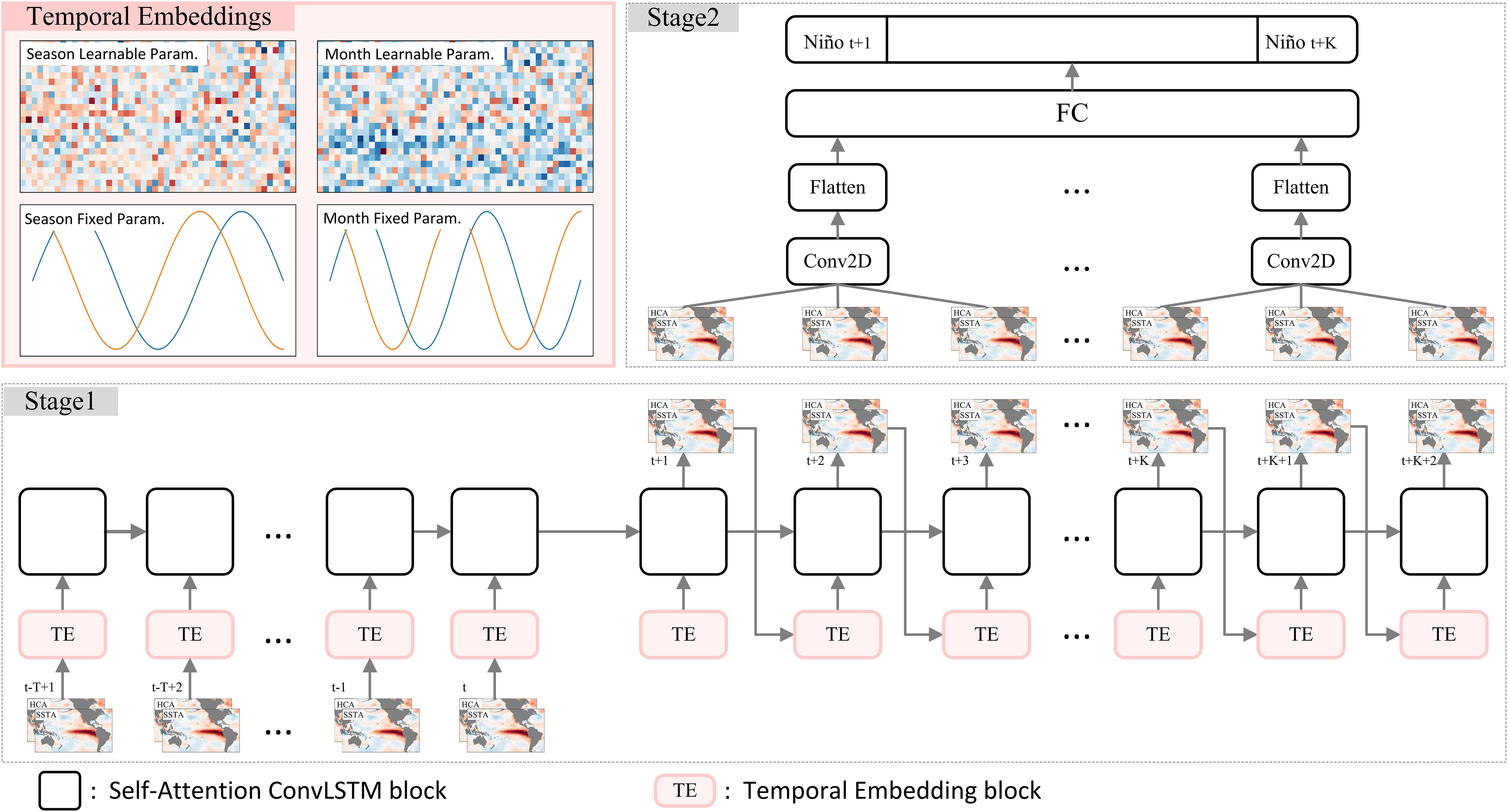
Figure 1 Architecture of the Two-Stage SpatioTemporal (TSST) prediction model for ENSO forecasting. Stage 1 (beneath the figure) illustrates the unfolded architecture of the autoregressive model based on the self-attention ConvLSTM network. The input comprises historical data of SSTA and HCA for T steps, while the output includes predicted SSTA and HCA for the future K+2 steps. At each step, the input undergoes a time encoding block that integrates the current meteorological feature with corresponding seasonal and monthly encoding features (details in the top-left corner of the figure). Stage 2 (depicted in the top-right corner) showcases the structure of the mapping model, where the predicted SSTA and HCA for the future K+2 steps from Stage 1 are grouped in sets of three consecutive steps and fed into the Stage 2 model. This data then undergoes convolution, pooling, flattening, fully connected layers, and is mapped to the corresponding Niño 3.4 value for that specific time step. In this study, T is set to 12, and K is set to 24. .
In the context of ENSO prediction, temporal information is comprised of seasons and calendar months information. Unified modeling of seasons and calendar months can help to capture different granularities of temporal information within the ENSO spatiotemporal sequence. Seasonal modeling is employed to capture coarse-grained temporal patterns, leveraging the distinct seasonal characteristics inherent in ENSO. On the other hand, calendar month modeling is introduced to capture finer-grained temporal information. Considering that the features between three consecutive months corresponding to the same season can vary, individual modeling of each calendar month is necessary. Focusing solely on modeling calendar months, without considering the coarse-grained information of seasons, may hinder the ability to capture similarities within the same season and differentiate features across different seasons. On the contrary, exclusive modeling seasons, while neglecting the fine-grained information of calendar months, may result in the inability to model similarities within the same calendar month and differentiate features across different calendar months.
Effectively encoding both components can enhance the model’s ability to capture ENSO dynamics, ultimately leading to improved predictive performance. To harness the potential of these two aspects, we proposes three distinct approaches for encoding calendar month and seasonal information: a fixed encoding method, a learnable parameter-based approach, and a hybrid method that combines fixed encoding with learnable parameters.
The fixed encoding approach involves utilizing trigonometric functions with periods of 12 and 4 to encode the calendar months and seasons, respectively. The periods 12 and 4 correspond to the twelve calendar months and four distinct seasons. The specific formulation is provided as Equation 4.
where i and j denote the index of the i-th calendar month and j-th season, respectively. This method can provide a stable temporal prior without the need for learning, but it lacks flexibility. In other words, the time embedding representation obtained from this encoding may not be the most optimal.
Considering that the dataset inherently contains both calendar month and season information, we can adopt the approach of learnable parameters. Specifically, distinct learnable parameters are assigned to each calendar month and season, allowing us to adaptively learn the feature representations of calendar months and seasons directly from the data. However, it comes with a higher learning difficulty and typically requires a substantial amount of data to achieve the best time embedding representation.
The advantage of the fixed encoding approach lies in its ability to provide a stable prior representation, thereby reducing the risk of model overfitting. On the other hand, the use of learnable parameters offers the benefits of greater flexibility and adaptability, enhancing expressive capabilities. In order to balance both stability and flexibility, we proposes an approach combining both encoding strategies. By using fixed periodic function encoding to provide a stable temporal prior, it reduces the learning difficulty associated with the parameterized encoding. This approach may yield better temporal embedding representations in situations where data is limited.
Self-Attention ConvLSTM Lin et al. (2020b) excels at capturing dependencies between distant and nearby regions simultaneously. It is constructed using multiple Self-attention ConvLSTM cells, as depicted in Supplementary Figure S2, where each cell combines the self-attention mechanism with the standard ConvLSTM Shi et al. (2015). The self-attention mechanism is a direct and efficient approach to modeling dependencies between distant regions, while the ConvLSTM employs convolutional operations instead of fully connected ones, enabling it to effectively capture both spatial and temporal dependencies. The convolutional operations, with their local connections and weight-sharing mechanism, are especially effective at modeling dependencies between nearby regions. This model cell is formulated as Equation 5.
where SA denotes the self-attention memory module. M denotes memory state. Details about self-attention memory module can be found in Supplementary Figure S2. At each time step, the current cell’s hidden state, Ht, is computed by filtering the input information, Xt, and forgetting certain information from the historical state, Ct−1. Initially, Htaggregates features only from spatially adjacent points. Htis then combined with distant node features using the SAM module. Additionally, during the application of the SAM module to Ht, relevant features from the historical memory Mt−1 are also aggregated, resulting in a comprehensive spatiotemporal representation
In stage 1, we predict future meteorological maps for a specific time horizon. However, our ultimate goal is to derive ENSO indicators, which presents challenges due to mapping relationships, resolution disparities, prediction errors, and the need for comprehensive feature inclusion. To overcome these challenges and improve the accuracy, we introduce a second-stage mapping network comprised of convolutional, pooling, and fully connected layers. This network bridges the gap between meteorological predictions and ENSO indicators, enhancing prediction accuracy and addressing the complexities of ENSO forecasting. It takes as input the meteorological features predicted by the first-stage model for the consecutive three months in the future and outputs the ENSO indicators for the future corresponding time steps. The computation formula for this network is represented by Equation 6.
Our research employs three distinct datasets: Coupled Model Intercomparison Project phase 5 (CMIP5) Giorgetta et al. (2013) dataset for training, Simple Ocean Data Assimilation (SODA) Carton and Giese (2008) dataset for validation, and Global Ocean Data Assimilation System (GODAS) Behringer and Xue (2004) dataset for testing. Detailed information can be found in Table 1 and Supplementary Table S1. In stage 1, in order to enhance computational efficiency and mitigate noise interference, we exclusively utilize SSTA and HCA within the spatial range of 55°S to 60°N and 95°E to 330°E. This region comprehensively covers the entire Pacific area, which is crucial for the formation and evolution of ENSO (Supplementary Figure S1).

Table 1 Details of the training, validation and testing dataset for Niño 3.4 prediction.
We construct samples using a sliding window approach. Firstly, we concatenate the data of each month in chronological order, resulting in a long sequence. Then, a window of length 12 months slides along this sequence from the beginning to the end with an interval of τ. Each sliding generates a sample. This approach generates samples with a certain degree of overlap between adjacent ones. The advantage lies in the increased sample quantity, effective exploitation of temporal information in the data, and enhanced data utilization. However, a drawback arises when neighboring samples exhibit significant overlap, leading to high redundancy between samples and potentially causing overfitting in the model, rendering training challenging. Therefore, the setting of τ needs to strike a balance between sample quality and correlation. Additionally, the choice of sampling interval τ must also balance the number of samples forecasted from different calendar months and the associated prediction difficulty.
In this study, the performance of the model is evaluated from the perspectives of correlation and accuracy between predicted and actual values. The evaluation metrics employed include Pearson Correlation Coefficient (PCC), Root Mean Squared Error (RMSE), and Mean Absolute Error (MAE). The calculation formulas for these metrics are represented by Equation 7.
where Y and denote the actual values and its respective means, while P and denote the predicted values and its corresponding means. The index l takes values from 1 to 24, indicating the number of lead months, and s and e are the start and end years of the data, respectively.
All experiments were conducted using the PyTorch deep learning framework. The models were trained on an NVIDIA A40 GPU using the Adam optimizer. The learning rate is set to 0.001, with a batch size of 2. The sliding window sampling interval τ is chosen as 5, and the maximum number of epochs is set at 40. In stage 1, the SAConvLSTM model consisted of 4 layers, with each layer having a feature dimension of 128, accompanied by 64 attention heads. The dimensions of the learnable embeddings for calendar months and seasons are (12, 24, 48) and (4, 24, 48) respectively. These embeddings are integrated by directly concatenating them with the original features. In Stage 2, the convolutional kernel size is set to 3 × 3, the number of nodes in the fully connected layer is 128, and a dropout rate of 0.1 is applied.
To demonstrate the effectiveness of our proposed TSST model in ENSO prediction, we conducted a comprehensive comparison with several representative benchmark methods, including numerical prediction approaches such as SINTEX-TEX Luo et al. (2008), CanCM3, CanCM4 (NMME Kirtman et al. (2014)), CCSM3, GFDL-are04, and GFDL-FLOR-A06, as well as deep learning methods like MSCNN Ye et al. (2021b), CNN Ham et al. (2019), ENSOTR Ye et al. (2021a) and Res-CNN Hu et al. (2021). The evaluation results are presented in Figure 2A, which depicts the correlation coefficients varying with lead months on the test dataset. The figure reveals declining correlation coefficients as lead months increase for all methods.
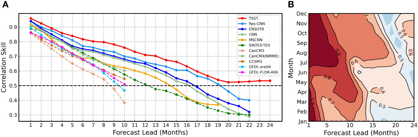
Figure 2 ENSO correlation skill TSST model. (A)The all-season correlation skill of Niño 3.4 as a function of forecast lead month in TSST model (red), Res-CNN model (dogerblue), ENSOTR model (blue), CNN model (darkseagreen) and other methods (the other colors). The validation period is between 1984 and 2017. Solid lines represent deep learning models, and dashed lines represent dynamical forecast systems. (B) The seasonality of correlation skills is further assessed as a function of lead time and calendar month for Niño 3.4, with contours of correlation skills exceeding the highlighted 0.5 value.
Traditional numerical prediction approaches perform well for the initial 10 lead months (correlation > 0.5), but their accuracy degrades more rapidly, limiting long-term predictions. In contrast, deep learning methods outperform traditional techniques by maintaining effective predictions for about 16-19 lead months, ensuring better long-term predictive outcomes.
Our proposed TSST method belongs to the category of deep learning-based approaches. However, it outperforms previous deep learning methods. Specifically, our method achieves significantly higher correlation coefficient values than previous deep learning-based methods across all 24 lead months. On average, there is an enhancement of 0.04 in the correlation coefficient. Notably, the improvements are even more significant for long-term forecasting. For instance, at the 22nd lead month, the correlation coefficient increases from 0.40 to 0.52. This could stem from the effective utilization of temporal information and evolving information embedded in HCA (Supplementary Figure S3). Furthermore, our approach consistently achieves correlation coefficients exceeding 0.5 across all 24 lead months. During the span of lead months from 19 to 24, the correlation coefficient is consistently maintained at approximately 0.52, with a slight upward trend. These findings collectively indicate that our model has the capability to capture the long-term evolutionary trends of ENSO, enabling an effective long-term forecasting. Moreover, these results demonstrate the model’s capacity to extend its forecasting horizon beyond the initial 24 lead months, encompassing even longer lead months with efficacy.
Figure 2B illustrates the correlation coefficients of our model’s predictions for each calendar month across lead months ranging from 1 to 24 on the test dataset. Generally, when the lead months are shorter, the prediction task is less challenging, leading to favorable prediction outcomes. On the contrary, as the lead months increase, the prediction difficulty escalates, resulting in less accurate predictions. Additionally, the difficulty of ENSO forecasting varies across different calendar months and is closely linked to the developmental stages of ENSO events. Starting from January and extending to April, ENSO is in its early developmental stage, resulting in relatively lower predictability. This might be attributed to the intricate interaction between sea surface temperatures and atmospheric circulation during this period, leading to the influence of multiple climatic variables on ENSO signals and subsequently weaker correlations. From May to August, ENSO reaches its mature phase, showing higher predictability. This is likely due to the gradual clarification of the relationship between sea surface temperature anomalies and atmospheric circulation, resulting in more pronounced event signals and stronger correlations. Moving on to September through December, corresponding to the middle-to-late declining phase of ENSO events, predictability remains relatively high. This could be attributed to the weaker interaction between sea surface temperatures and atmospheric circulation, diminishing interference in ENSO signals, a decreased impact of other climatic patterns on predictions, and reduced noise levels. Similar observations were also made in the predictions for Niño 3 and Niño 4 (Supplementary Figures S6, S7).
To analysis the contributions of different regions of distinct variables to the final prediction, we employ Shapley Additive Explanations (SHAP) Lundberg and Lee (2017). SHAP calculates the marginal contribution of adding a specific feature to a model and then considers the average marginal contributions of that feature across all possible feature permutations. This average is referred to as the SHAP value, representing the contribution of the feature to the final prediction. In comparison to typical interpretability methods, SHAP offers greater flexibility and produces more stable results. The findings related to SSTA are shown in Figure 3. Similar results about HCA and fixed temporal embeddings are displayed in Supplementary Figures S10 and S11. When the lead month is small, the contribution near the Niño 3.4 region is significant, while contributions from other regions are minimal. However, with larger lead months, the contribution near the Niño 3.4 region diminishes, and contributions from other regions increase, especially in the vicinity of points including (305°E, 50°N), (275°E, 0°), and (100°E, 0°), which become particularly significant.
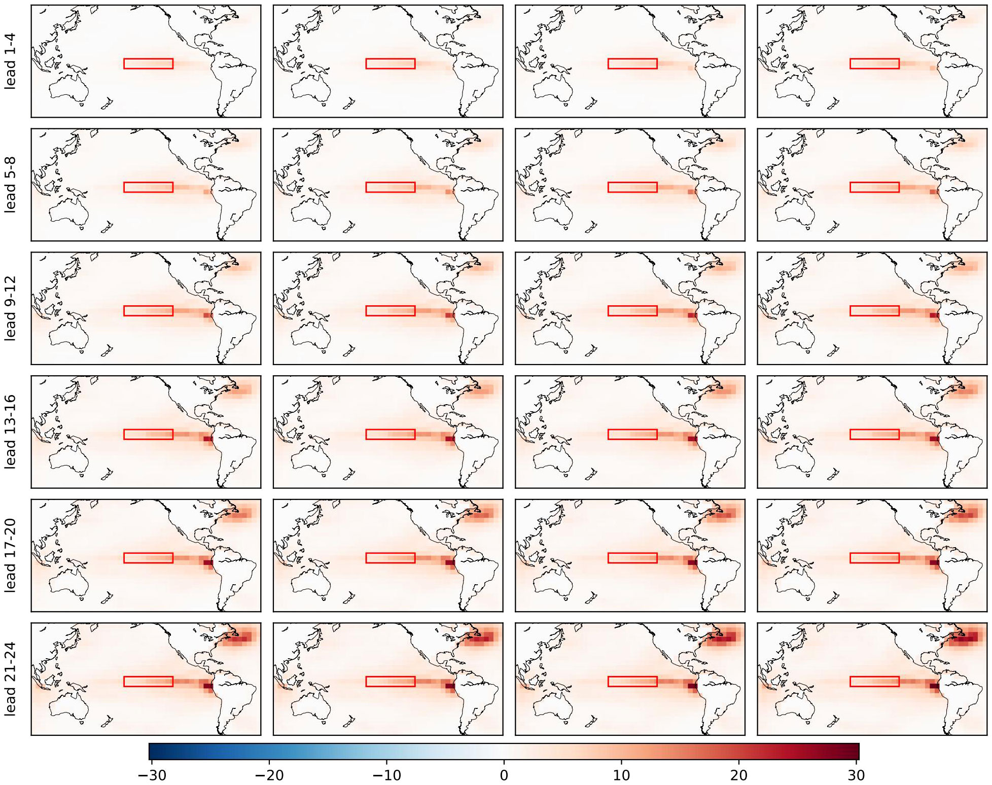
Figure 3 The absolute SHAP value distribution of SSTA from different locations for various lead months in predicting the Niño3.4 results. A higher SHAP value indicates a more significant contribution of that location to the final prediction. The red box indicates the Niño3.4 region.
The contributions at ( °E, °) and ( °E, °) are likely associated with the Pacific Meridional Mode (PMM) Fan et al. (2021) and the Indian Ocean Dipole (IOD), both of which are signals correlated with ENSO. However, there is limited evidence supporting a relationship between the North Atlantic and ENSO. The contribution at ( °E, °N) appears challenging to explain. Below, we attempt a brief explanation. Firstly, it’s important to note that our model predicts the Niño 3.4 index, not ENSO events. The occurrence of ENSO events in the testing set is relatively low. Therefore, the contribution analysis results indicate the average contribution of the predicted Niño 3.4 index in the testing set. This is different from directly analyzing the contribution of predicting ENSO events. Secondly, in long-term forecasts, our model tends to underestimate the intensity of ENSO events compared to their actual strength. This suggests that our model finds it challenging to predict the occurrence of ENSO events in the long term. Hence, the contribution analysis here is more inclined towards the contribution to the normal variation of the Niño 3.4 index, rather than the contribution during abnormal periods, i.e., the occurrence of ENSO events. PMM or IOD generally has a significant impact on the occurrence of ENSO events, but the contributions to the changes in the Niño 3.4 index may differ. Moreover, contributions may include causal and non-causal components. For instance, there might be a strong causal relationship between PMM and ENSO, leading to a larger contribution from the eastern equatorial Pacific’s sea surface temperature and heat content characteristics. On the other hand, contributions from the North Atlantic region in long-term predictions might stem from non-causal relationships, where both factors change simultaneously to some extent but lack a causal connection. This could explain why, in long-term predictions, the contribution from the North Atlantic region might be greater than that of the PMM or IOD.
In order to evaluate the importance of different components in ENSO prediction, we performed ablation experiments for each component. To keep fair, all the comparison experimental data, including parameters setting, training set and test set are the same as TSST-based ENSO prediction.
To investigate the impact of different variables, we compares the performance of a model using solely SSTA (Stage 1 (SSTA)) with a model employing both SSTA and HCA (Stage 1 (SSTA+HCA)). The experimental results is depicted in Figure 4. From the outcomes, it is evident that in short-term forecasting, the two models exhibit comparable performance, with the model employing both SSTA and HCA slightly outperforming the model using solely SSTA. However, in long-term forecasting, the model incorporating both SSTA and HCA demonstrates markedly better performance than the model solely utilizing SSTA. This discrepancy could be attributed to the fact that, in the short term, the influence of SSTA on ENSO is more direct, whereas the impact of heat content is relatively minimal. The utilization of solely SSTA might already capture short-term ENSO variations effectively. In contrast, during long-term forecasting, the development of ENSO may be influenced by multiple factors, and the information encapsulated within SSTA might be limited and prone to disturbances from other climatic patterns. Thus, it may fall short in supporting ENSO’s long-term forecasting. HCA, as a reflection of the ocean’s energy reserves, can better depict the ocean’s response over large time scales, offering more stable meteorological information over the long term. Furthermore, HCA could also play a role in delayed response Huang and Kinter (2002), implying that changes in oceanic heat content might manifest in sea surface temperature after a certain period. This delayed response might be more dominate in long-term forecasting, thereby enhancing the performance of models utilizing HCA in such scenarios.
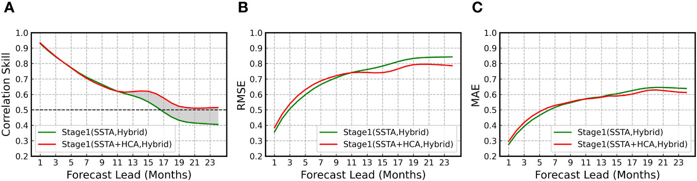
Figure 4 Comparison of ENSO prediction skills between the control and sensitivity experiments regarding meteorological variables. The all-season correlation (A), root mean square error (B) and mean absolute error (C) of Niño 3.4 as a function of forecast lead month in stage 1 using only SSTA and using both SSTA and HCA. The validation period is between 1984 and 2017.
In order to further investigate the specific roles of calendar month and season information in ENSO prediction, we conducted experiments in stage 1 using several different embedding approaches for calendar months and seasons, as outlined earlier. The experimental outcomes, illustrated in Figure 5, portray the performance of the aforementioned models on the testing dataset across different lead months. From the figure, it can be observed that the performance of all four models generally decreases as the lead months increase. However, the rate of performance decay varies across different stages. Short-term predictions may rely more on the inherent features of the input SSTA and HCA, with weaker dependence on seasonal and calendar month features. In short-term predictions, the stage1(no-time) model performs the best, followed by the stage1(fixed-time) and stage1(learn-time) models. The stage1(hybrid) model performs the worst, possibly due to the stronger influence of meteorological factors on short-term ENSO variations. This trend may be attributed to the fact that short-term variations in ENSO are more directly influenced by meteorological factors, with a relatively weaker relationship to changes in calendar months and seasons. Omitting calendar month and season information might assist the model in capturing short-term changes more effectively. Integrating additional information into short-term predictions might disturb the model’s focus on primary meteorological variations, leading to poorer performance.

Figure 5 Comparison of ENSO prediction skills between the control and sensitivity experiments regarding temporal embedding. The all-season correlation (A), root mean square error (B) and mean absolute error (C) of Niño 3.4 as a function of forecast lead month in stage 1 for four temporal embedding strategies: no temporal embedding, fixed temporal embedding, learnable temporal embedding, and a hybrid approach combining fixed and learnable temporal embedding. The validation period is between 1984 and 2017. In the ultimate TSST model, during stage 2, inputs comprise combined predictions from Stage 1 (no-time) and Stage 1 (hybrid). SSTA and HCA are both used in these four models.
Long-term predictions may rely more on seasonal and calendar month features, with weaker dependence on the features of the input SSTA and HCA. In long-term predictions, the stage1(hybrid) model performs the best, followed by the stage1(fixed-time) and stage1(learn-time) models. It seems that models utilizing calendar month and season embedding representations consistently outperform those that do not incorporate this information. This phenomenon could be attributed to the fact that, in long-term predictions, the direct influence of meteorological factors on ENSO variations diminishes, while the relationship with changes in calendar months and seasons becomes relatively stronger. Not incorporating calendar month and season embedding representations might result in the model’s inability to capture these critical temporal dependencies, leading to poorer long-term predictive performance.
Furthermore, models using fixed and learnable embeddings show comparable performance, slightly exceeding fixed embeddings. This might stem from the dataset’s size constraining learnable parameters’ ability to capture strong calendar month and season embeddings. With a larger dataset, the advantage of learnable parameters could become more clear. Moreover, the hybrid embedding outperforms fixed and learnable embeddings. Fixed embeddings offer a stable temporal prior but struggle with dynamic data. Learnable embeddings can adapt to dynamic changes but require more data for reliable learning. The hybrid method combines both strengths, using fixed embeddings for stability and learnable parameters for data-specific variations. This strategy captures ENSO’s long-term patterns and enhances predictions even with limited data. Embeddings of calendar months and seasons by the stage 1 (hybrid) model are shown in Supplementary Figures S4 and S5, effectively highlighting distinct patterns for each month and season.
The performance enhancement from hybrid is more remarkable than that from HCA. As indicated by the red curves in Figures 4 and 5, our Stage1(SSTA+HCA, Hybrid) model has shown excellent performance in long-term predictions. To further analysis whether the improvement in performance is more significant due to HCA or the Hybrid method, we conducted experiments by separately removing HCA and Hybrid components. The experimental results are illustrated by the green curve in Figure 4 and the cyan curve in Figure 5. From the results, in long-term predictions, the Stage1(SSTA, Hybrid) model outperforms the Stage1(SSTA+HCA) model. Also, observing the shaded areas in Figures 4 and 5, it’s evident that the performance improvement from Stage1(SSTA+HCA) to Stage1(SSTA+HC,Hybrid) is more remarkable than the improvement from Stage1(SSTA,Hybrid) to Stage1(SSTA+HCA,Hybrid). These observations suggest that the performance enhancement from the Hybrid method is more significant than that from HCA, further affirming the effectiveness of the Hybrid approach.
In our approach, the first stage employs a spatiotemporal sequence prediction model based on SAConvLSTM, utilizing historical meteorological spatiotemporal factors to predict future ones. The second stage utilizes a mapping network based on convolution, pooling, and fully connected layers to map the predicted future meteorological spatiotemporal factors from Stage 1 to the corresponding future ENSO indicator at each time step. It is important to note that in Stage 1, to leverage the short-term predictive advantage of SAConvLSTM (no-time) and the long-term predictive advantage of SAConvLSTM (hybrid), we employ the outputs of both models as inputs to the Stage 2 model, resulting in the final TSST model.
To validate the contributions of each stage in our two-stage model, we conducted an ablation experiment about each stage on the TSST model. The results, depicted in Figure 6, illustrate the variation of correlation coefficients, root mean squared errors, and mean absolute errors of the stage1(hybrid) model, stage1(notime) model, and the Stage 2 model (TSST) over different lead months. Table 2 provides detailed experimental results for these models at lead times of 3, 6, 9, 12, 15, 18, 21, and 24 months.
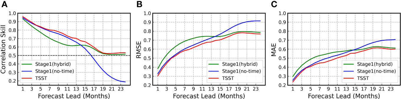
Figure 6 Comparisons of ENSO prediction skills between the control and sensitivity experiments regarding model stage. The all-season correlation (A), root mean square error (B) and mean absolute error (C) of Niño 3.4 as a function of forecast lead month for three different models: the stage 1 model without temporal embedding, the stage 1 model with hybrid temporal embedding, and the stage 2 model. The validation period is between 1984 and 2017. Description of the figure.
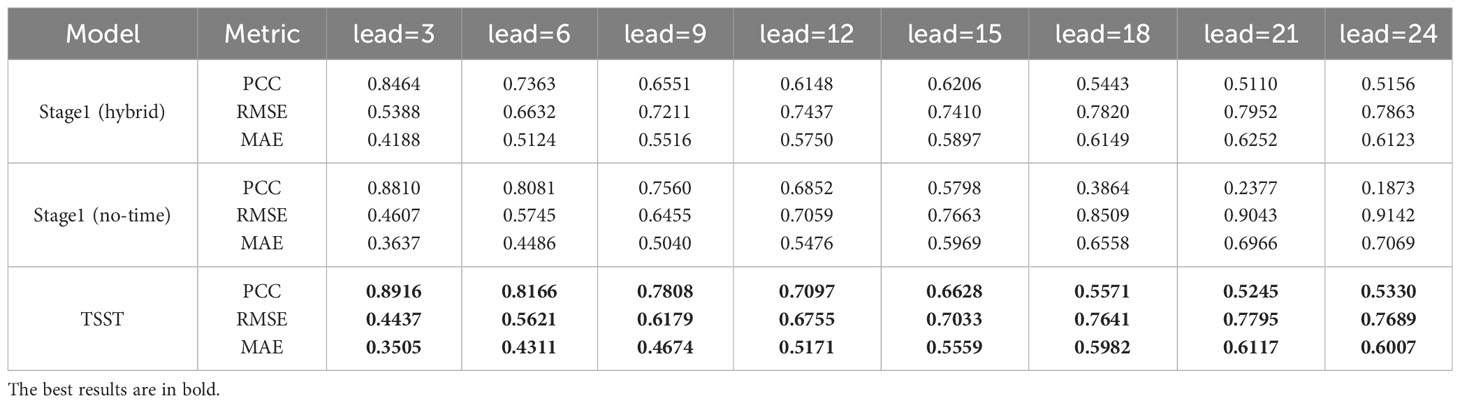
Table 2 Comparison among predictions made using only Stage1, only Stage2 and TSST models; here prediction validations are performed using GODAS dataset for 3, 6, 9, 12, 15, 18, 21 and 24 month lead times.
The experimental outcomes indicate that the Stage 2 model slightly outperforms the two models from Stage 1 in both short-term and long-term predictions, combining the strengths of short-term and long-term predictions from the Stage 1 models. Furthermore, the Stage 2 model demonstrates substantial performance improvement in mid-term predictions compared to the Stage 1 models. This suggests that the two Stage 1 models possess complementary predictive characteristics in the middle term, and the Stage 2 model effectively extracts and utilizes this complementary information to achieve superior prediction results.
In ENSO prediction, our primary purpose lies in predicting whether an ENSO event will occur and assessing its intensity. Therefore, it’s necessary to further analyze the prediction results of typical ENSO events. Additionally, the spring prediction barrier have a significant impact on ENSO prediction. Hence, it is essential to delve deeper into the analysis of how these springtime affect the model.
Figure 7 depicts the comparison between our model’s predicted outcomes and the actual results for lead times of 1, 3, 6, 9, 12, 15, 18, and 21 months on the test dataset. From the observations, it is evident that the predicted Niño 3.4 curves for all lead times exhibit similar inflection points as the actual curves. This indicates that our model effectively captures the changing trends of the Niño 3.4 index. For lead times within 3 months, the predicted Niño 3.4 curves closely match the fluctuations of the actual curves. However, for lead times beyond 9 months, the amplitude of fluctuations in the predicted curves is smaller than that in the actual curves, indicating a convergence of extreme values. Additionally, the convergence increases with longer lead times. Similar phenomenon is also observed in other methods. This could be attributed to the relatively lower proportion of extreme values in real data, causing the model’s predictions to incline toward the sample mean when faced with greater prediction difficulty at longer lead times. To mitigate this convergence at longer lead times, possible strategies include adjusting the weights of the loss function or implementing a loss function that is sensitive to outliers. Addressing this issue holds particular significance for enhancing the accuracy of ENSO event prediction. We leave this as a topic for future research.
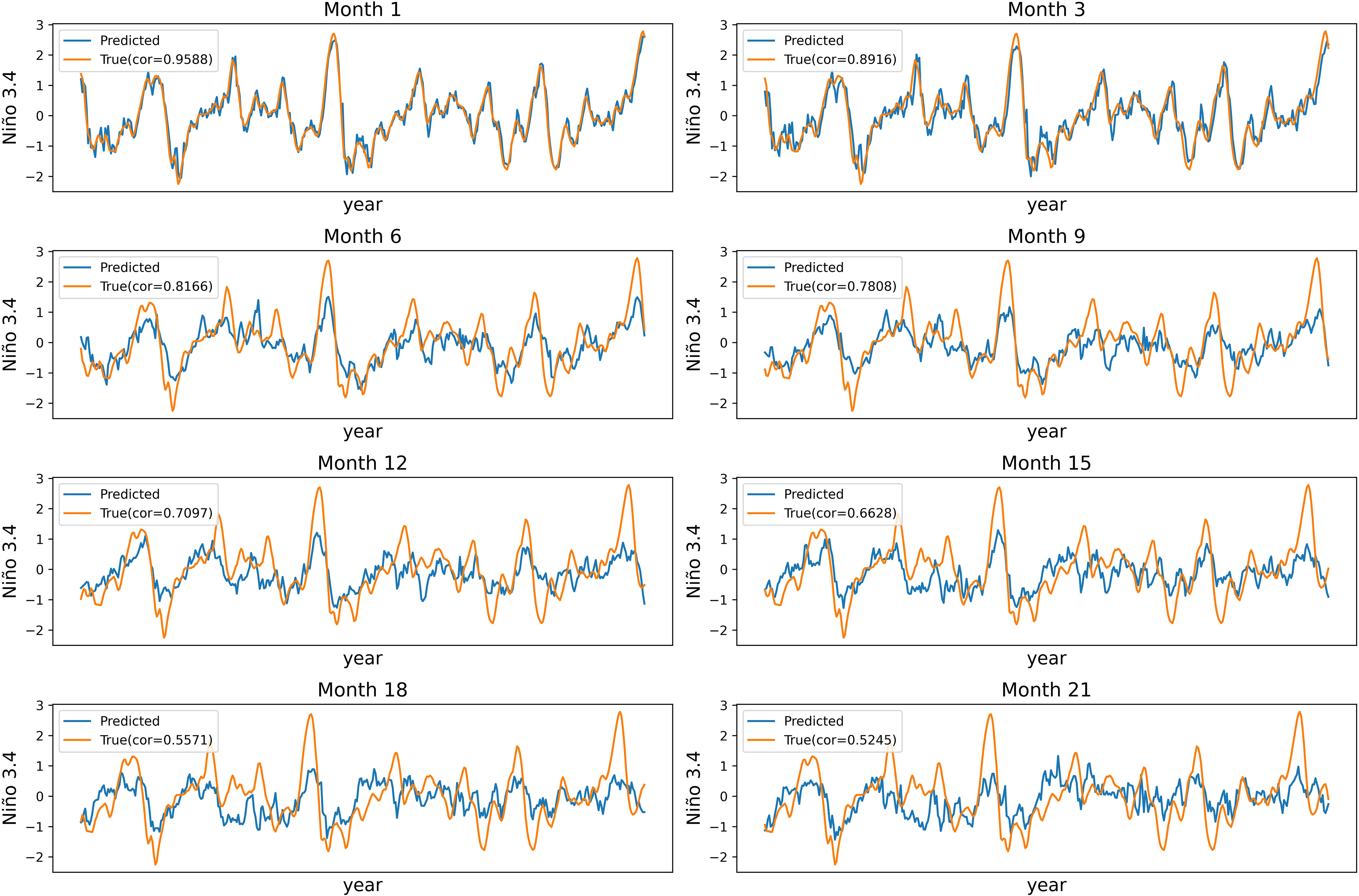
Figure 7 Niño 3.4 prediction by TSST model and observation from 1982 to 2017 at a lead time of 1, 3, 6, 9, 12, 15, 18, 21 months. Cor means correlation skill.
In order to investigate the seasonal impacts, we conduct a study on the performance of the model when starting predictions from 12 different calendar months. The Niño 3.4 results are presented in Figure 8. Notably, the analysis involves two independent variables: the lead months and the position of the spring months within the preceding 24 months. The dependent variable is a singular correlation coefficient. Then, our analysis will primarily focus on addressing two key questions. By the way, similar observations were also made in the predictions for Niño 3 and Niño 4 (Supplementary Figures S8, S9).
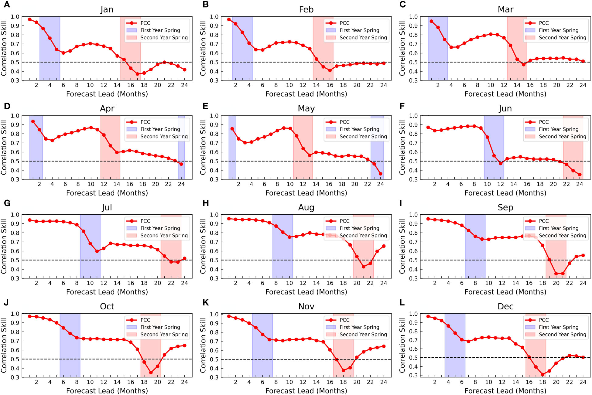
Figure 8 ENSO correlation skill in the TSST model when starting predictions from different calendar months. The correlation skill of Niño 3.4 as a function of the forecast lead month (red line). The first spring calendar month within the lead 24 months (blue shade). The second spring calendar month within the lead 24 months (red shade). (A–L) correspond to January through December.
As evident from Figure 8, regardless of the starting calendar month for predictions, the model consistently exhibits lower prediction results at spring months within the leading 24 months (as indicated by the shaded region in the figure) compared to the predictions at adjacent lead months. This phenomenon confirms the presence of the spring predictability barrier.
From Figure 8, variations in prediction outcomes are evident when starting predictions from different calendar months, particularly related to the spring months within the leading 24 months. Within this period, there are two instances of spring months. To elucidate, let’s first consider the impact of the first occurrence of spring, denoted by the blue-shaded region in the figure. Regardless of the calendar month chosen as the starting point for predictions, the correlation coefficient curve experiences accelerated decay as it approaches the first spring month. Notably, within this month, the curve descends most rapidly. Once past the first spring month, the correlation coefficient curve essentially stabilizes, exhibiting either sluggish decline or, in some instances, a slight improvement in performance for certain starting months. However, the correlation coefficients following the spring month are notably lower than those preceding it. In essence, the first occurrence of the spring month rapidly diminishes the model’s predictive performance, and this diminishing effect continues to influence predictions across subsequent lead months.
To analyze this, we will provide an explanation from the model’s perspective. We employed an autoregressive predictive model, which entails feeding the model with the meteorological factors (specifically SSTA and HCA) of the preceding month, enabling it to predict the subsequent month’s meteorological factors. During optimization, the process involves computing a loss between the predicted and actual meteorological factors for the current month, followed by gradient backpropagation for continual refinement of the model’s parameters. For regular calendar months (non-spring months), this approach performs well, enabling the model to learn the temporal evolution of ENSO phenomena. However, the scenario changes when it comes to spring months. Notably, in comparison to other months, the true meteorological factors at spring months exhibit significant noise, yielding a low signal-to-noise ratio concerning ENSO signals. In our model, the noise exists in both input and label. This introduces two challenges. Firstly, noise of considerable magnitude infiltrates the process of loss computation, gradient backpropagation, and parameter updates. Secondly, the accuracy of predicting meteorological factors for the current time step diminishes, contributing to substantial noise. As a result, when these noisy predicted meteorological factors for the present time step are utilized as inputs for subsequent time steps, the noise persists and propagates, leading to inaccuracies in subsequent predictions. This elucidates why the diminishing effect persists throughout subsequent lead months. Furthermore, there’s a minor improvement in model performance following the first spring month, which may relate to the model’s inherent bias correction capabilities.
As for the second spring, marked by the red-shaded area in the figure, a similar trend can be observed. However, there is a noticeable difference. After the second spring, the correlation coefficient curve experiences relatively substantial improvements when predictions commence from certain months, such as August, September, October, November, and so on. This suggests that when initiating predictions from these months, the model is more robust after the second spring. Accounting for the feature of the model, during the second spring month, despite the presence of noise in both input and label, the model maybe has learned some crucial spatiotemporal patterns of ENSO evolution. Consequently, the model has developed a degree of bias correction ability, which mitigates the impact of noise, leading to enhanced predictions for the subsequent lead months.
In order to analyze the performance of our model in predicting typical El Niño and La Niña events, we present the results in Figure 9, where our model’s predictions for the La Niña event in 1988, El Niño events in 1997 and 2015 are depicted. All three predictions were initiated from August of the preceding year. From the figure, it is evident that our model successfully captures the ENSO phenomena corresponding to the respective years, although the predicted intensities appear to be lower than the actual ENSO intensities.
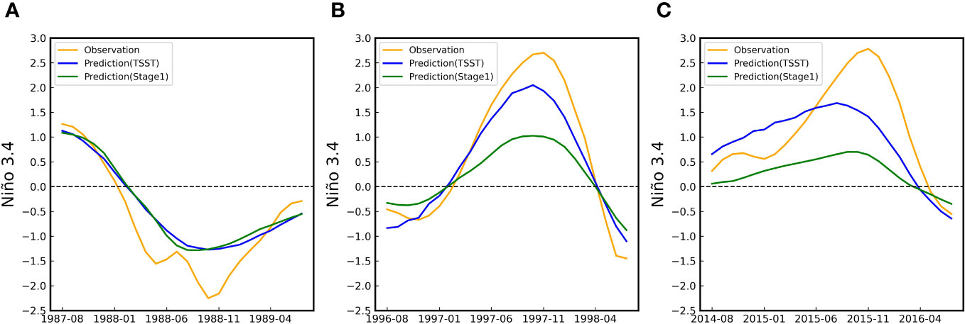
Figure 9 Prediction examples made for typical ENSO events. Analyzed (orange), TSST-stage1 model predicted (green) and TSST model predicted (blue) Niño 3.4 for the 1988-1989 La Niña event (A), 19971998 El Niño event (B) and 2015-2016 El Niño event (C). All three start predictions from the calendar month of August.
Furthermore, for the El Niño event in 1998, Figure 10 illustrates the comparison between our Stage 1 model’s predicted sea surface temperatures in the Pacific region at lead times of 3, 12, and 18 months, against the actual observed sea surface temperatures. The results demonstrate that our model indeed captures the evolving patterns of sea surface temperatures in the Pacific region. However, as the lead time increases, the predicted sea surface temperature fluctuations exhibit smaller amplitudes compared to the observed sea surface temperature fluctuations.
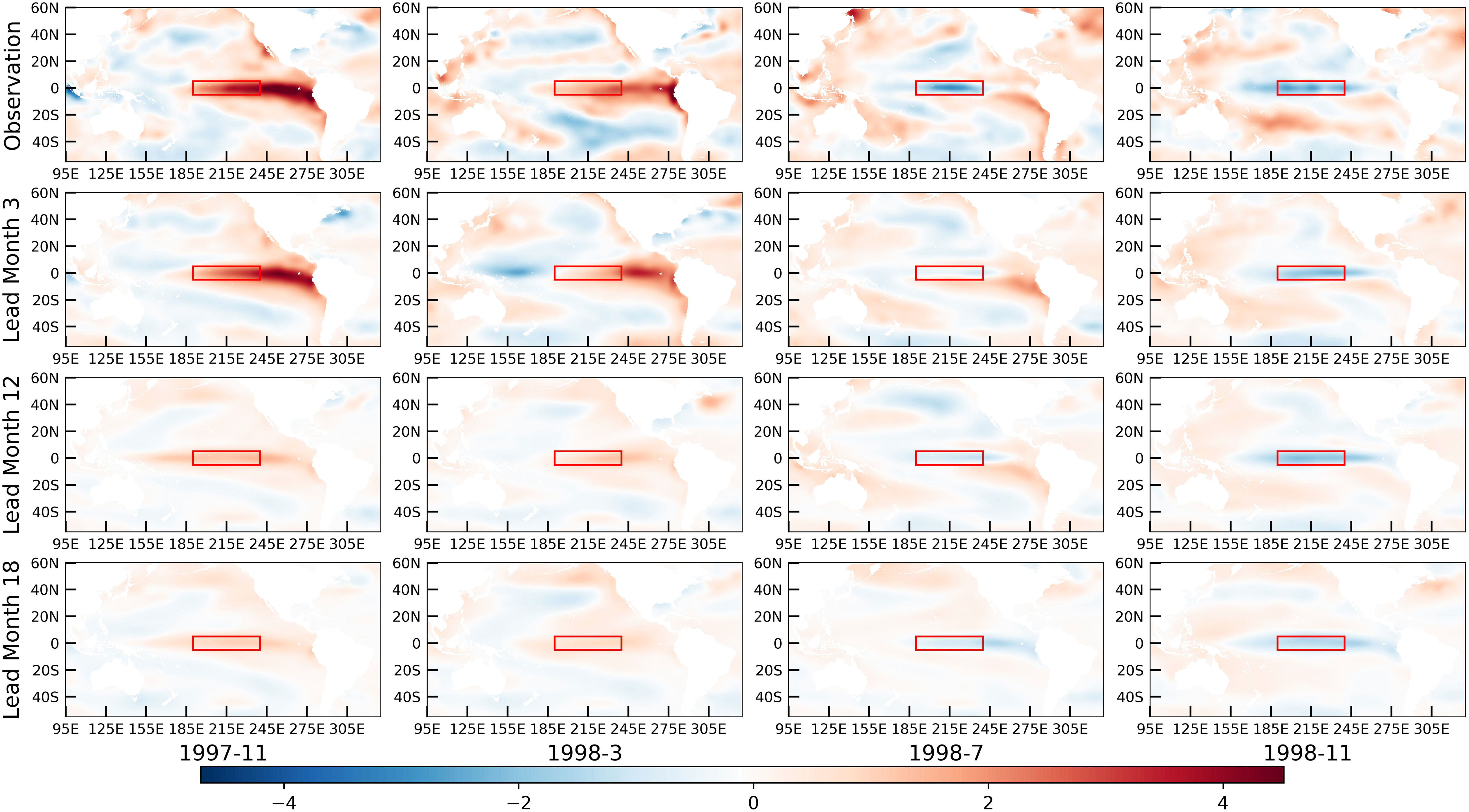
Figure 10 Prediction example for spatiotemporal evolutions over the Pacific region (55°S to 60°N and 95°E to 330°E). The first row depicts SSTA heatmaps for the months of November 1997, March 1998, July 1998, and November 1998. The second, third, and fourth rows illustrate corresponding SSTA heatmaps predicted by TSST model for lead times of 3, 12, and 18 months, respectively. The red box indicates the Niño3.4 region.
The aim of incorporating time modeling in deep learning is generally to enhance the model’s perception to temporal features in the data. One potential way of deep learning methods to accommodate various seasonal and the quasi-periodic nature is to automatically encode the time features and regularize the learned representations in the frequency domain to preserve certain consistency observed in the spectrum. In this paper, we model the calendar month-seasonal characteristics of ENSO instead of directly addressing its quasi-periodic features. We outline the differences between these two aspects, providing a detailed explanation. Additionally, we briefly discuss challenges associated with directly modeling the quasi-periodic nature of ENSO.
In the third paragraph of the Introduction, we theoretically elaborate on the calendar month and seasonality of ENSO. Corresponding to real-world data, as depicted in Figure 11 for the Niño 3.4 index spanning from 1982 to 2017, we illustrate the variations during spring, summer, autumn, and winter. The overall trend observed from the figure indicates that, generally, during the spring season, ENSO events tend to be in their initial phase with relatively weak signals, as evidenced by smaller values of the Niño 3.4 index. In contrast, during autumn, ENSO events are in their mature phase, characterized by stronger signals and larger values of the Niño 3.4 index. Notably, strong El Niño events occurring at distant intervals in 1983, 1998, and 2016 all commenced in spring, developed in summer, matured in autumn, and declined in winter, concluding in the following spring. This season-specific pattern is referred to as seasonal characteristics. However, periodic modeling of ENSO focuses on the time intervals between occurrences, such as the temporal gaps between these three strong El Niño events. There exists differences between these two features, and the seasonal features do not necessarily manifest solely in the annual periodic components.
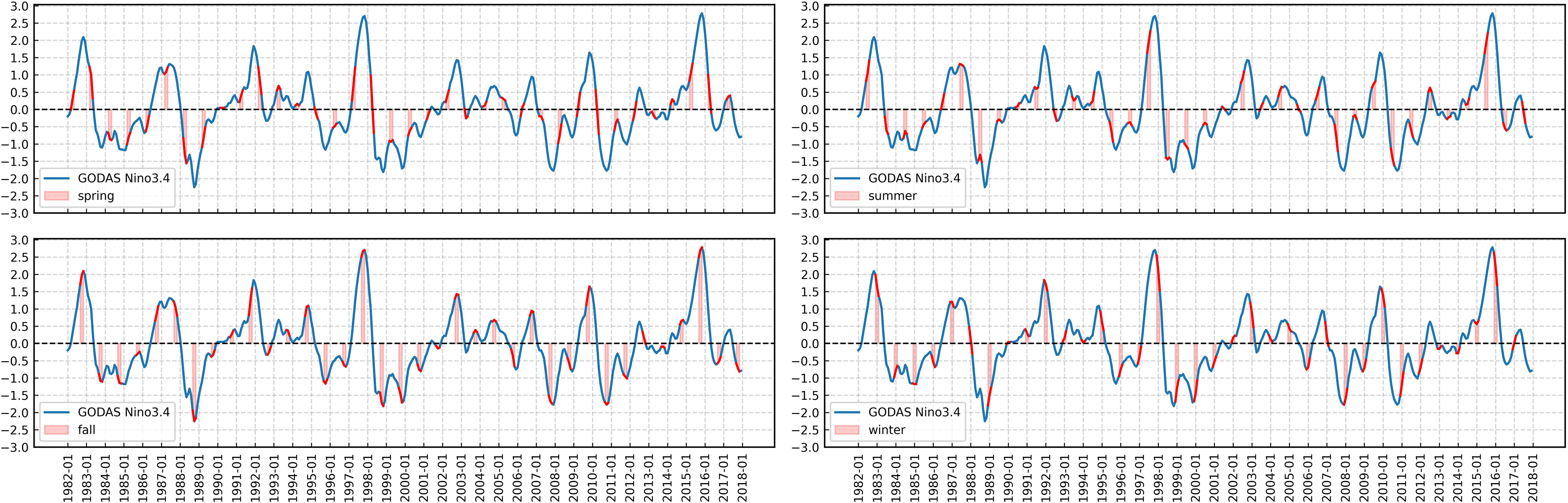
Figure 11 Niño 3.4 index values of the spring, summer, fall, and winter seasons spanning from 1982 to spring 2017. The red shaded intervals denote the monthly periods corresponding to respective season. The first row corresponds to the spring and summer seasons, while the second row corresponds to the fall and winter seasons.
The short-term periodicity of ENSO events is non-constant, typically ranging between 2 to 7 years Timmermann et al. (2018). Some studies, conducted through dominant frequency state analysis, have confirmed the existence of long-term climate cycles in the ENSO process Bruun et al. (2017). Employing Morlet wavelet transformation on the Niño 3.4 index to shift to the frequency domain, as depicted in Figure 12, allows for the analysis of various frequency components and their intensities of the ENSO signal. Subsequently, encoding is considered for frequency components with relatively high intensities. Although this approach effectively addresses the issue of variable periodicity, an inherent challenge remains - the need to determine an additional starting point. For example, for a two-year periodic component, encoding initialized from the first year versus the second year may yield significantly divergent results. To the best of our knowledge, there is currently no effective means of directly modeling the quasi-periodicity of ENSO in deep learning, presenting an intriguing and worthwhile subject for further exploration.
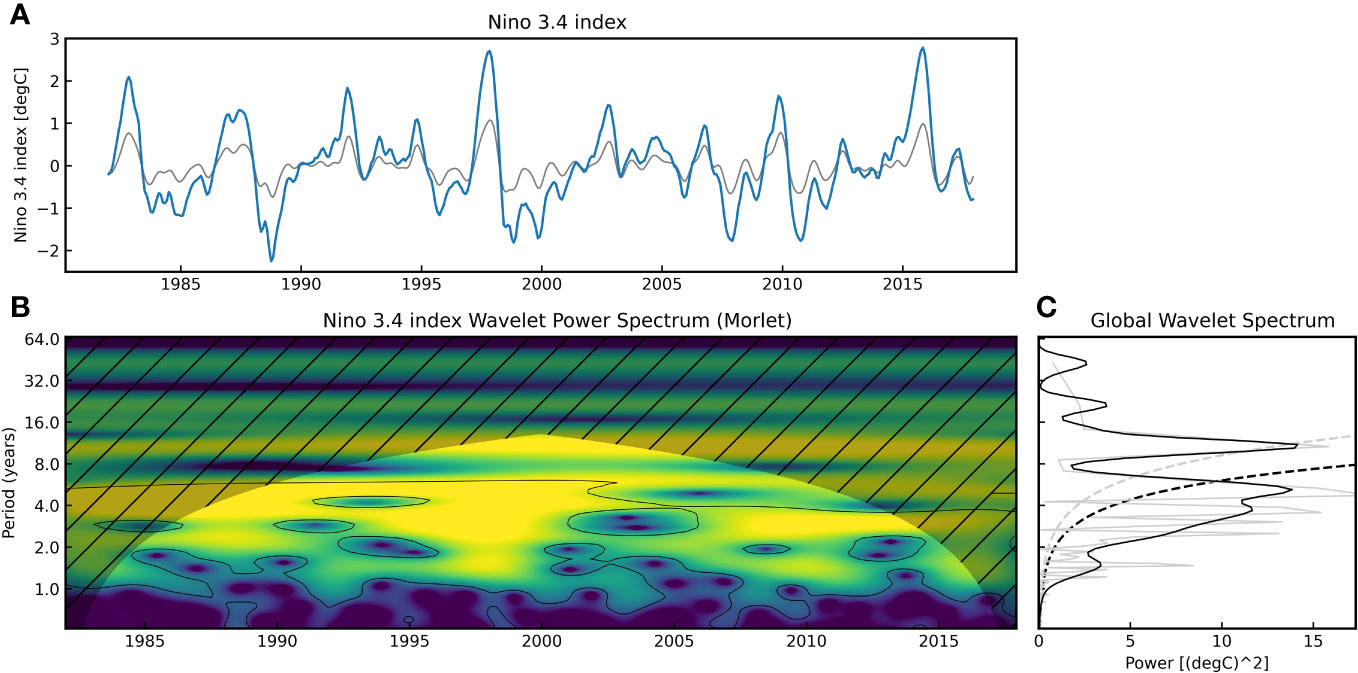
Figure 12 (A) Niño 3.4 index series (blue solid line) and the wavelet inverse transform time series (gray solid line)from 1982 to 2017. (B) Normalized wavelet power spectrum analysis of the Niño 3.4 index is conducted using the Morlet wavelet (ω0 = 6) as a function of time and Fourier equivalent wave periods (years). The contour lines in black, relative to a red noise stochastic process (α = 0.77), indicate regions with a confidence level exceeding 95%. The shaded region with left-sloping lines represents the Cone of Influence (COI) for the wavelet transform. (C) Global wavelet power spectrum (black solid line) and Fourier power spectrum (gray solid line). Dashed lines denote the 95% confidence level.
The spatiotemporal evolution patterns of ENSO are often embedded in meteorological spatiotemporal sequence data, which possess complex spatial and temporal characteristics. These attributes include local range, long-range spatiotemporal correlations, calendar month patterns, and seasonal patterns. An efficient ENSO prediction model needs to effectively extract spatiotemporal features from the meteorological data to capture the evolution patterns of ENSO. To achieve this goal, we proposes a Two-Stage SpatioTemporal (TSST) autoregressive model for ENSO prediction. In Stage 1, the SAConvLSTM model is used to capture both short-range and long-range spatiotemporal dependencies. Additionally, two methods, namely periodic function encoding and learnable parameter encoding, are used to model calendar month and seasonal information. In Stage 2, a CNN-based model is employed to map the meteorological factors predicted in Stage 1 to indicator factors. Experiments demonstrate that our model can effectively predict ENSO on a lead time of 24 months and partially alleviate the spring prediction barrier issue.
While the proposed method in this study has achieved promising ENSO prediction performance, there are still aspects that require further investigation and enhancement.
1. Firstly, how to alleviate the issue of model contraction? When the forecast horizon is extensive, the model tends to underestimate the intensity of ENSO events. This could be attributed to the scarcity of samples corresponding to ENSO events in real scenarios. Adjusting the weights of the loss function or incorporating a loss function sensitive to outlier values could potentially mitigate the issue of model contraction when dealing with larger lead months. Such adjustments hold significant implications for enhancing the predictive accuracy of ENSO events.
2. Secondly, how to further alleviate the spring prediction barrier? From the data perspective, the most direct approach is to apply denoising techniques to the spring meteorological factors, such as using predictions from a trained model to replace actual observations. From the model perspective, a preliminary idea is to explore methods for designing a model with enhanced bias correction capabilities, such as incorporating learnable parameters.
3. Lastly, extending the model’s applicability to other meteorological issues is vital. The spatiotemporal dependencies at both short and long distances, as well as the attributes related to calendar months and seasons, are prevalent in various meteorological problems, such as the Indian Ocean Dipole (IOD) phenomenon Ling et al. (2022). Exploring how to apply our method to other domains of meteorological problems is an area that merits further research consideration.
The original contributions presented in the study are included in the article/Supplementary Material. Further inquiries can be directed to the corresponding author.
CR: Conceptualization, Formal Analysis, Investigation, Methodology, Software, Validation, Visualization, Writing – original draft, Writing – review & editing. ZS: Conceptualization, Funding acquisition, Supervision, Writing – review & editing, Methodology. WZ: Funding acquisition, Data curation, Writing – review & editing. A-AL: Funding acquisition, Project administration, Data curation, Writing – review & editing. ZW: Funding acquisition, Project administration, Resources, Writing – review & editing.
The author(s) declare financial support was received for the research, authorship, and/or publication of this article. This work was supported in part by the National Key Research and Development Program of China (2021YFF0704000) and the National Natural Science Foundation of China (U22A2068, U23A20320).
The authors declare that the research was conducted in the absence of any commercial or financial relationships that could be construed as a potential conflict of interest.
All claims expressed in this article are solely those of the authors and do not necessarily represent those of their affiliated organizations, or those of the publisher, the editors and the reviewers. Any product that may be evaluated in this article, or claim that may be made by its manufacturer, is not guaranteed or endorsed by the publisher.
The Supplementary Material for this article can be found online at: https://www.frontiersin.org/articles/10.3389/fmars.2024.1334210/full#supplementary-material
Adams R. M., Chen C.-C., McCarl B. A., Weiher R. F. (1999). The economic consequences of enso events for agriculture. Climate Res. 13, 165–172. doi: 10.3354/cr013165
Alexander M. A., Bladé I., Newman M., Lanzante J. R., Lau N.-C., Scott J. D. (2002). The atmospheric bridge: The influence of enso teleconnections on air–sea interaction over the global oceans. J. Climate 15, 2205–2231. doi: 10.1175/1520-0442(2002)015⟨2205:TABTIO⟩2.0
Behringer D., Xue Y. (2013). Evaluation of the global ocean data assimilation system at INCOIS: The tropical Indian Ocean. Ocean Model. 69, 123–135. doi: 10.1016/j.ocemod.2013.05.003
Broni-Bedaiko C., Katsriku F. A., Unemi T., Atsumi M., Abdulai J.-D., Shinomiya N., et al. (2019). El niño-southern oscillation forecasting using complex networks analysis of lstm neural networks. Artif. Life Robotics 24, 445–451. doi: 10.1007/s10015-019-00540-2
Bruun J. T., Allen J. I., Smyth T. J. (2017). Heartbeat of the s outhern o scillation explains enso climatic resonances. J. Geophysical Research: Oceans 122 (8), 6746–6772. doi: 10.1002/2017JC012892
Cai W., Santoso A., Wang G., Yeh S.-W., An S.-I., Cobb K. M., et al. (2015). Enso and greenhouse warming. Nat. Climate Change 5, 849–859. doi: 10.1038/nclimate2743
Carton J. A., Giese B. S. (2008). A reanalysis of ocean climate using simple ocean data assimilation (soda). Monthly weather Rev. 136, 2999–3017. doi: 10.1175/2007MWR1978.1
Chapanov Y., Ron C., Vondrak J. (2017). Decadal cycles of earth rotation, mean sea level and climate, excited by solar activity. Acta Geodyn. Geomater 14, 241–250. doi: 10.13168/AGG.2017.0007
Cheng L., Trenberth K. E., Fasullo J. T., Mayer M., Balmaseda M., Zhu J. (2019). Evolution of ocean heat content related to enso. J. Climate 32, 3529–3556. doi: 10.1175/JCLI-D-18-0607.1
Dilley M., Heyman B. N. (1995). Enso and disaster: Droughts, floods and el niño/southern oscillation warm events. Disasters 19, 181–193. doi: 10.1111/j.1467-7717.1995.tb00338.x
Dommenget D., Yu Y. (2016). The seasonally changing cloud feedbacks contribution to the enso seasonal phase-locking. Climate Dynamics 47, 3661–3672. doi: 10.1007/s00382-016-3034-6
Fan H., Huang B., Yang S., Dong W. (2021). Influence of the pacific meridional mode on enso evolution and predictability: Asymmetric modulation and ocean preconditioning. J. Climate 34, 1881–1901. doi: 10.1175/JCLI-D-20-0109.1
Fiedler P. C. (2002). Environmental change in the eastern tropical pacific ocean: review of enso and decadal variability. Mar. Ecol. Prog. Ser. 244, 265–283. doi: 10.3354/meps244265
Geng H., Wang T. (2021). Spatiotemporal model based on deep learning for enso forecasts. Atmosphere 12, 810. doi: 10.3390/atmos12070810
Giorgetta M. A., Jungclaus J., Reick C. H., Legutke S., Bader J., Böttinger M., et al. (2013). Climate and carbon cycle changes from 1850 to 2100 in mpi-esm simulations for the coupled model intercomparison project phase 5. J. Adv. Modeling Earth Syst. 5, 572–597. doi: 10.1002/jame.20038
Ham Y.-G., Kim J.-H., Kim E.-S., On K.-W. (2021). Unified deep learning model for el niño/southern oscillation forecasts by incorporating seasonality in climate data. Sci. Bull. 66, 1358–1366. doi: 10.1016/j.scib.2021.03.009
Ham Y.-G., Kim J.-H., Luo J.-J. (2019). Deep learning for multi-year enso forecasts. Nature 573, 568–572. doi: 10.1038/s41586-019-1559-7
Hu J., Weng B., Huang T., Gao J., Ye F., You L. (2021). Deep residual convolutional neural network combining dropout and transfer learning for enso forecasting. Geophysical Res. Lett. 48, e2021GL093531. doi: 10.1029/2021GL093531
Huang B., Kinter III J. L. (2002). Interannual variability in the tropical Indian ocean. J. Geophysical Research: Oceans 107, 20–21. doi: 10.1029/2001JC001278
Jin D., Kirtman B. P. (2010). The impact of enso periodicity on north pacific sst variability. Climate dynamics 34, 1015–1039. doi: 10.1007/s00382-009-0619-3
Kirtman B. P., Min D., Infanti J. M., Kinter J. L., Paolino D. A., Zhang Q., et al. (2014). The north american multimodel ensemble: phase-1 seasonal-to-interannual prediction; phase-2 toward developing intraseasonal prediction. Bull. Am. Meteorological Soc. 95, 585–601. doi: 10.1175/BAMS-D-12-00050.1
Kumar K. K., Rajagopalan B., Cane M. A. (1999). On the weakening relationship between the Indian monsoon and enso. Science 284, 2156–2159. doi: 10.1126/science.284.5423.2156
Lestari R. K., Koh T.-Y. (2016). Statistical evidence for asymmetry in enso–iod interactions. Atmosphere-Ocean 54, 498–504. doi: 10.1080/07055900.2016.1211084
Lin I.-I., Camargo S. J., Patricola C. M., Boucharel J., Chand S., Klotzbach P., et al. (2020a). Enso and tropical cyclones. In El Niño Southern Oscillation in a changing climate. (Wiley Online Library) 17, 377–408. doi: 10.1002/9781119548164.ch17
Lin Z., Li M., Zheng Z., Cheng Y., Yuan C. (2020b). Self-attention convlstm for spatiotemporal prediction. In Proc. AAAI Conf. Artif. intelligence. 34, 11531–11538. doi: 10.1609/aaai.v34i07.6819
Ling F., Luo J.-J., Li Y., Tang T., Bai L., Ouyang W., et al. (2022). Multi-task machine learning improves multi-seasonal prediction of the Indian ocean dipole. Nat. Commun. 13, 7681. doi: 10.1038/s41467-022-35412-0
Lopez H., Kirtman B. P. (2014). Wwbs, enso predictability, the spring barrier and extreme events. J. Geophysical Research: Atmospheres 119, 10–114. doi: 10.1002/2014JD021908
Lundberg S. M., Lee S.-I. (2017). A unified approach to interpreting model predictions. Adv. Neural Inf. Process. Syst. 30.
Luo J.-J., Masson S., Behera S. K., Yamagata T. (2008). Extended enso predictions using a fully coupled ocean–atmosphere model. J. Climate 21, 84–93. doi: 10.1175/2007JCLI1412.1
Lv A., Fan L., Zhang W. (2022). Impact of enso events on droughts in China. Atmosphere 13 (11), 1764. doi: 10.3390/atmos13111764
Manzello D. P., Enochs I. C., Bruckner A., Renaud P. G., Kolodziej G., Budd D. A., et al. (2014). Galápagos coral reef persistence after enso warming across an acidification gradient. Geophysical Res. Lett. 41, 9001–9008. doi: 10.1002/2014GL062501
McPhaden M. J. (2003). Tropical pacific ocean heat content variations and enso persistence barriers. Geophysical Res. Lett. 30 (9), 1480. doi: 10.1029/2003GL016872
McPhaden M. J., Zhang X., Hendon H. H., Wheeler M. C. (2006). Large scale dynamics and mjo forcing of enso variability. Geophysical Res. Lett. 33 (16), 702. doi: 10.1029/2006GL026786
Rajagopalan B., Cook E., Lall U., Ray B. K. (2000). Spatiotemporal variability of enso and sst teleconnections to summer drought over the United States during the twentieth century. J. Climate 13, 4244–4255. doi: 10.1175/1520-0442(2000)013⟨4244:SVOEAS⟩2.0.CO;2
Ren H.-L., Zuo J., Jin F.-F., Stuecker M. F. (2016). Enso and annual cycle interaction: The combination mode representation in cmip5 models. Climate Dynamics 46, 3753–3765. doi: 10.1007/s00382-015-2802-z
Shi X., Chen Z., Wang H., Yeung D.-Y., Wong W.-K., Woo W.-C. (2015). Convolutional lstm network: A machine learning approach for precipitation nowcasting. Adv. Neural Inf. Process. Syst. 28.
Stuecker M. F., Timmermann A., Jin F.-F., McGregor S., Ren H.-L. (2013). A combination mode of the annual cycle and the el niño/southern oscillation. Nat. Geosci. 6, 540–544. doi: 10.1038/ngeo1826
Tang Y., Zhang R.-H., Liu T., Duan W., Yang D., Zheng F., et al. (2018). Progress in enso prediction and predictability study. Natl. Sci. Rev. 5, 826–839. doi: 10.1093/nsr/nwy105
Timmermann A., An S.-I., Kug J.-S., Jin F.-F., Cai W., Capotondi A., et al. (2018). El niño–southern oscillation complexity. Nature 559, 535–545. doi: 10.1038/s41586-018-0252-6
Tobler W. (2004). On the first law of geography: A reply. Ann. Assoc. Am. Geographers 94, 304–310. doi: 10.1111/j.1467-8306.2004.09402009.x
Tziperman E., Cane M. A., Zebiak S. E. (1995). Irregularity and locking to the seasonal cycle in an enso prediction model as explained by the quasi-periodicity route to chaos. J. Atmospheric Sci. 52, 293–306. doi: 10.1175/1520-0469(1995)052⟨0293:IALTTS⟩2.0.CO;2
Tziperman E., Stone L., Cane M. A., Jarosh H. (1994). El niño chaos: Overlapping of resonances between the seasonal cycle and the pacific ocean-atmosphere oscillator. Science 264, 72–74. doi: 10.1126/science.264.5155.72
Wang C., Fiedler P. C. (2006). Enso variability and the eastern tropical pacific: A review. Prog. oceanography 69, 239–266. doi: 10.1016/j.pocean.2006.03.004
Wang H., Hu S., Li X. (2023). An interpretable deep learning enso forecasting model. Ocean-LandAtmosphere Res. 2, 0012. doi: 10.34133/olar.0012
Yan J., Mu L., Wang L., Ranjan R., Zomaya A. Y. (2020). Temporal convolutional networks for the advance prediction of enso. Sci. Rep. 10 (1), 8055. doi: 10.1038/s41598-020-65070-5
Ye F., Hu J., Huang T.-Q., You L.-J., Weng B., Gao J.-Y. (2021a). Transformer for ei niño-southern oscillation prediction. IEEE Geosci. Remote Sens. Lett. 19, 1–5. doi: 10.1109/LGRS.2021.3100485
Ye M., Nie J., Liu A., Wang Z., Huang L., Tian H., et al. (2021b). Multi-year enso forecasts using parallel convolutional neural networks with heterogeneous architecture. Front. Mar. Sci. 8. doi: 10.3389/fmars.2021.717184
Zhao J., Luo H., Sang W., Sun K. (2023). Spatiotemporal semantic network for enso forecasting over long time horizon. Appl. Intell. 53, 6464–6480. doi: 10.1007/s10489-022-03861-1
Keywords: El Niño-Southern Oscillation (ENSO), deep learning for ENSO prediction, self-attention ConvLSTM, temporal embeddings, spring prediction barrier
Citation: Rui C, Sun Z, Zhang W, Liu A-A and Wei Z (2024) Enhancing ENSO predictions with self-attention ConvLSTM and temporal embeddings. Front. Mar. Sci. 11:1334210. doi: 10.3389/fmars.2024.1334210
Received: 06 November 2023; Accepted: 22 January 2024;
Published: 12 February 2024.
Edited by:
Weimin Huang, Memorial University of Newfoundland, CanadaReviewed by:
John T. Bruun, University of Exeter, United KingdomCopyright © 2024 Rui, Sun, Zhang, Liu and Wei. This is an open-access article distributed under the terms of the Creative Commons Attribution License (CC BY). The use, distribution or reproduction in other forums is permitted, provided the original author(s) and the copyright owner(s) are credited and that the original publication in this journal is cited, in accordance with accepted academic practice. No use, distribution or reproduction is permitted which does not comply with these terms.
*Correspondence: Zhengya Sun, emhlbmd5YS5zdW5AaWEuYWMuY24=
Disclaimer: All claims expressed in this article are solely those of the authors and do not necessarily represent those of their affiliated organizations, or those of the publisher, the editors and the reviewers. Any product that may be evaluated in this article or claim that may be made by its manufacturer is not guaranteed or endorsed by the publisher.
Research integrity at Frontiers
Learn more about the work of our research integrity team to safeguard the quality of each article we publish.