Biomass estimations of cultivated kelp using underwater RGB images from a mini-ROV and computer vision approaches

Seaweed farming is the fastest-growing aquaculture sector worldwide. As farms continue to expand, automated methods for monitoring growth and biomass become increasingly important. Imaging techniques, such as Computer Vision (CV), which allow automatic object detection and segmentation can be used for rapid estimation of underwater kelp size. Here, we segmented in situ underwater RGB images of cultivated Saccharina latissima using CV techniques and explored pixel area as a tool for biomass estimations. Sampling consisted of underwater imaging of S. latissima hanging vertically from a cultivation line using a mini-ROV. In situ chlorophyll a concentrations and turbidity (proxies for phytoplankton and particle concentrations) were monitored for water visibility. We first compared manual length estimations of kelp individuals obtained from the images (through manual annotation using ImageJ software). Then, we applied CV methods to segment and calculate kelp area and investigated these measurements as a robust proxy for wet weight biomass. A strong positive linear correlation (r² = 0.959) between length estimates from underwater image frames and manual measurements from the harvested kelp was observed. Using unsupervised learning algorithms, such as mean shift clustering, colour segmentation and adaptive thresholding from the OpenCV package in Python, kelp area was segmented and the number of individual pixels in the contour area was counted. A positive power relationship was found between length from manual measurements with CV-derived area (r² = 0.808) estimated from underwater images. Likewise, CV-derived area had a positive power relationship with wet weight biomass (r² = 0.887). When removing data where visibility was poor due to high turbidity levels (mid-June), the power relationship was stronger between CV-derived area estimates and the field measurements (r² = 0.976 for wet weight biomass and r² = 0.979 for length). These results show that robust estimates of cultivated kelp biomass in situ are possible through kelp colour segmentation. However, we demonstrate that the quality of CV post-processing and accuracy of the model are highly dependent of environmental conditions (e.g. turbidity and chlorophyll a concentrations). The establishment of these technologies has the potential to offer scalability of production, efficient real-time monitoring of sea cultivation and improved yield predictions.

1 Introduction

Cultivated seaweed is the fastest-growing aquaculture sector worldwide (~6% y^-1) and a multibillion-dollar industry, comprising half of global mariculture production (Duarte et al., 2021). Seaweed farming has the potential to provide a sustainable, low trophic source of food (and feed) for a world approaching 10 billion by 2050 and can potentially be used as a nature-based solution for climate change mitigation and nutrient remediation (Duarte et al., 2021; van Dijk et al., 2021). The positive impact of seaweed aquaculture can help society to achieve many of the United Nations Sustainable Development Goals (UNSDGs) – from eliminating hunger and climate change mitigation, to economic growth, and improvement of life under water (Duarte et al., 2021; Hossain et al., 2021; Alleway, 2023).

While seaweed aquaculture has a long history in Asia (over a thousand years) (Hwang et al., 2019), which is responsible for 99% of worldwide production, sea cultivation of kelp has only recently become established in Europe (last 5-15 years). Norway, with its long coastline and favourable seaweed growing conditions, has the potential to be a major player as the European industry develops. In Norway alone, the number of licenses for seaweed cultivation has increased from 54 in 2014 to 511 in 2020, revealing the increased interest in seaweed farming (Albrecht, 2023). Predictions suggest the expansion of seaweed cultivation up to 2 × 10⁷ tonnes per year by 2050 (Olafsen et al., 2012; Skjermo et al., 2014; Broch et al., 2017), although there are some discussion about how realistic these projections are (Albrecht, 2023).

Although market demand for seaweed is generally increasing in Europe, Norwegian seaweed aquaculture is not yet profitable. One major reason for this is a lack of automation regarding seedling production, farm operations, monitoring, harvesting and processing of biomass at a large scale. Thus, as seaweed producers scale-up, it is important that they are able to maximise their yields at sea, while minimising production costs. To achieve this goal, a holistic understanding of the environmental conditions influencing macroalgal growth and the onset of biofouling is necessary to achieve biomass of consistent quality and yield. Accurately predicting the total biomass at harvest is also vital for planning the processing of the biomass. To date, kelp biomass measurements, biofouling inspections and environmental monitoring are still largely done by hand, which is time-consuming, labour intensive and cannot easily build up a holistic picture that is representative of the whole farm. Automation of kelp farm monitoring has the potential to revolutionize this aspect of the industry. The more automated and frequent monitoring is, the faster the pace of knowledge acquisition for optimising growth at sea, predicting yield and planning harvest and processing logistics.

Cost-effective monitoring of wild kelp has been performed in pilot studies using Red-Green-Blue (RGB) cameras (Bewley et al., 2012) or hyperspectral imaging by air using aerial drones/airplanes Volent et al. (2007) and from underwater platforms using remotely operated underwater vehicle (ROVs) (Summers et al. (2022). However, very little research has been done using underwater robot monitoring (autonomous underwater vehicles, AUVs, and ROVs) in kelp farms. Biomass growth has been assessed using AUVs with a split-beam acoustic echosounder (Fischell et al., 2019) and a sideward scanner to monitor the macroalgae growth in a kelp farm (Stenius et al., 2022). However, they are more appropriate for seaweed species that possess pneumatocysts (e.g. Macrocystis pyrifera), due to enhanced acoustic returns, and not for commercial species from Norway (mostly Saccharina latissima and Alaria esculenta) (Bell et al., 2020). Visual inspections are still necessary, though, for monitoring the kelp health and for robust estimation of biomass measurements, given that strong currents can underestimate these values by changing the direction of the kelp in the water (Bell et al., 2020). Moreover, AUVs cannot operate everywhere. They are less suited to areas that are heavily populated (near the shore) due to acoustic interference, and have a high collision and entanglement risk, which can lead to damage of the farm. They are also very expensive and require technical personnel for operation. Due to the tight space between kelp lines (maximum of a few meters), small and light underwater robots, such as portable drones (uncrewed surface vehicles, USV) (Zolich et al., 2022) and manually controlled mini-ROVs can offer a low risk assessment of the environmental conditions within the farm. The small, portable, mini-ROV Blueye model X3 (Blueye Robotics, Norway) was chosen in this study because of its user-friendly operability, making it manoeuvrable enough for easy operation in the tight spaces of a kelp farm, while at the same time providing sufficient power to operate in coastal conditions. It is also affordable (~ US$ 12k for the Blueye X3 drone + basic kit), making it an easily available option for seaweed farmers.

The aim of this study was to provide a proof-of-concept for in situ biomass estimation of cultivated S. latissima derived from underwater RGB imaging and computer vision (CV) techniques. For that, we compared manual length estimations to the ones obtained from images through human supervision, then, we applied CV methods to estimate kelp area and used these measurements as a proxy for wet weight biomass. To our knowledge, this is the first attempt where in situ biomass estimations from images are validated against field-measured, harvested biomass data. We show that robust estimates of cultivated kelp biomass in situ are possible through lamina colour segmentation, although we demonstrate that the quality of CV post-processing and accuracy of the model are highly dependent of environmental conditions, such as the colour of the water, turbidity, natural illumination and current velocities. The establishment of these technologies will offer scalability of production, efficient real-time monitoring of farm cultivation and improved yield predictions.

2 Methods

2.1 Study area and sampling methods

Fieldwork was carried out at the Seaweed Solutions kelp farm, Måsskjæra, in Frøya, an island located off the coast of mid-Norway (Trøndelag region) (63°44.62’N 8°52.76’E) (Figure 1). Frøya island is a biodiversity-rich area with strong water mixing due to internal waves, strong winds and tidal currents (Fragoso et al., 2021). The hydrography of the region is characterized by two different currents: the Norwegian Coastal Current (NCC) located above the Norwegian Atlantic Current (NAC). NCC is a result of freshwater runoff from Norwegian fjords comprising several rivers outflow in each fjord (Skagseth et al., 2011), while the NAC is a warm nutrient-rich water mass located below the NCC that occasionally intrudes to the surface in spring and summer (Skagseth et al., 2011) (Figure 1A). Because of the influence of the NAC, the area is highly productive regarding fisheries and aquaculture activities, with high economical revenue to Norway (Tiller et al., 2015; Ervik et al., 2018).

Figure 1

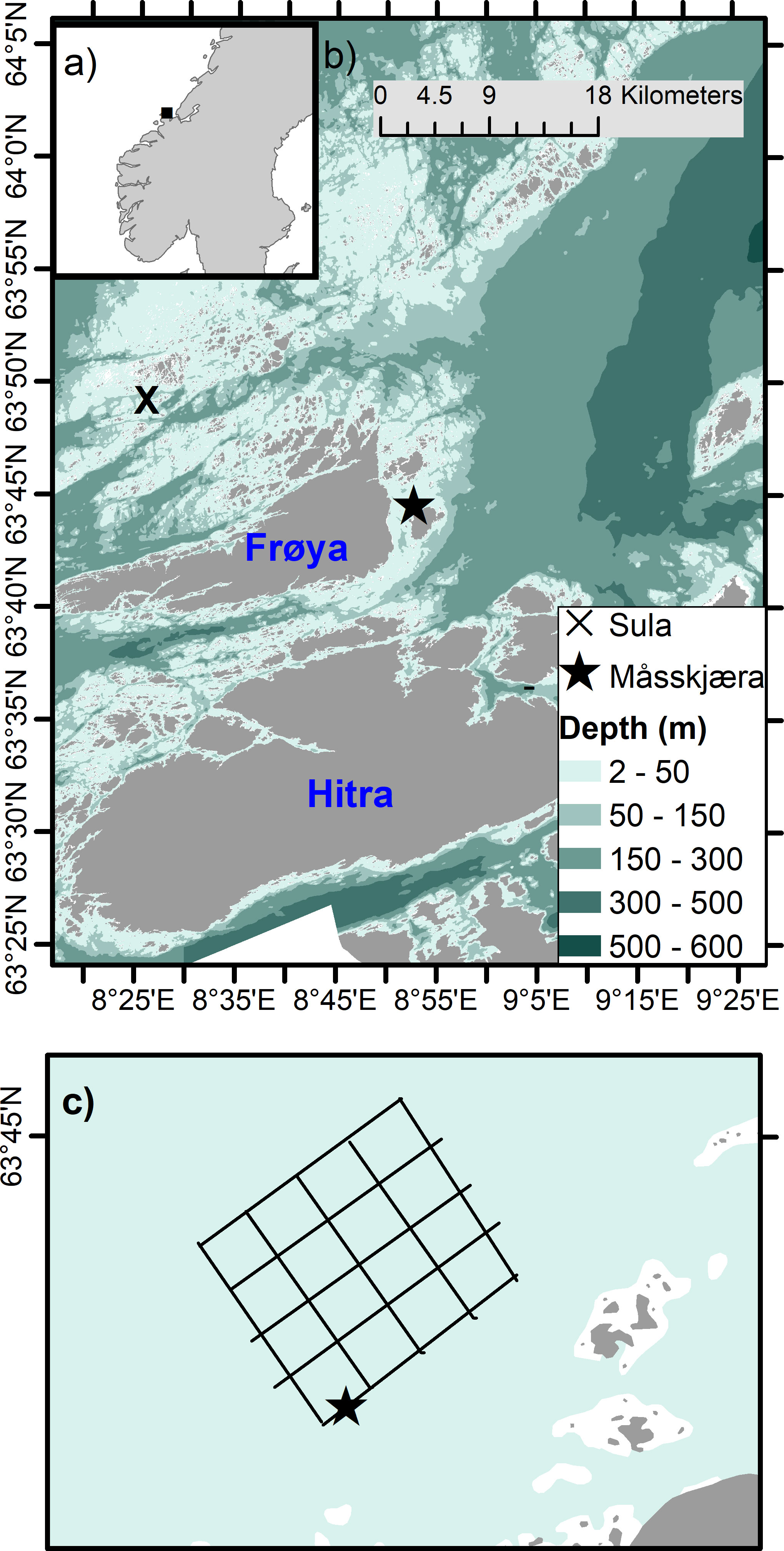
Figure 1 Map showing (A) Norway, and the coast of Trøndelag (mid-Norway, square) and (B) the island of Frøya and the location of Måsskjæra seaweed farm, and Sula meteorological station (where wind data were collected). (C) Illustration of the Måsskjæra seaweed farm, showing the collection site (star symbol).

Måsskjæra is a semi-exposed farm location sheltered from westerly and southerly wind directions and exposed to north-eastly winds (Førde et al., 2016) (Figure 1). Due to the shelter protection provided by the mainland and surrounding islands, wave height does not exceed 2 meters. The depth where the farm is located ranges from 10 - 35 m. The farm size is approximately 400 × 400 m and is based on a horizontal longline system that is divided into approximately 16 cultivation squares. S. latissima was cultivated on 100 m long substrate lines (14 mm diameter) that were seeded by wrapping them with cultivation twine (2 mm twisted polyester). The cultivation depth was between 2 and 5 m and was achieved by placing buoyancy in the middle of the 100 m substrate lines. Lines were cultivated with a spacing of approximately 1 m distance.

Sampling consisted of underwater imaging of a single kelp (S. latissima) cultivation line (~25 m in length) located at the edge of the farm and at ~ 2-5 m depth (Figures 1B, C). The monitored seaweed line was deployed in November 2021. Sampling occurred every 2 - 4 weeks within the later stages of the main growing season (from March to June 2022, 7 sampling times in total, Table 1). This allowed imaging and sampling during distinct development stages of S. latissima, from young sporophytes in March to ‘bushy canopy” in June, to test the method on kelp lines with a range of sizes and growth densities. Sampling was, where possible, carried out at low tide (slack water) to minimise current speeds in order to obtain images of S. latissima specimens oriented as vertical as possible. Sampling during high tide could also have been an option but, due to logistical reasons (boat and personnel availability), low tide was chosen in order to maintain consistency. In practice, however, ideal conditions for video recording (low tides) were not possible on all sampling days due to the logistical difficulties of arriving and deploying the ROV during the exact time of slack water (e.g. weather conditions and boat logistics) (Table 1).

Table 1

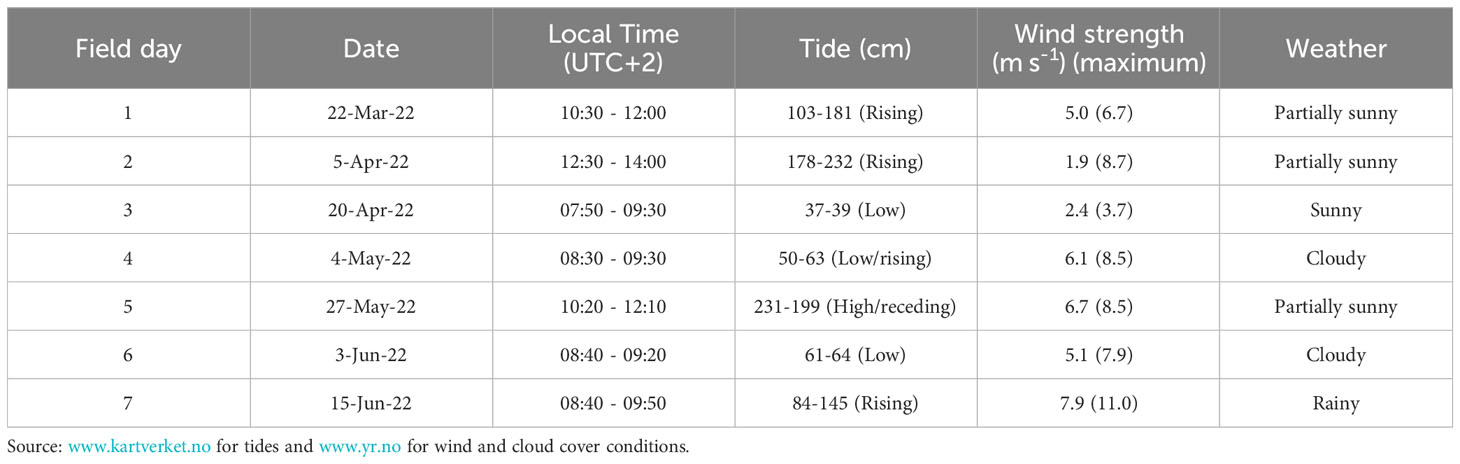
Table 1 Date, local Norwegian time, tidal conditions (cm), average and maximum wind speed (from Sula meteorological station, see methods) and cloud cover (Ørland meteorological station) for each video recording and sampling day at Måsskjæra.

Prior to recording underwater video, an aluminium-based hand-made checkerboard plate (30 × 20 cm) was placed at the start of the cultivation line for size reference. The plate was weighted in an attempt to keep it vertical during underwater videos. Additionally, red plastic strips were attached to the same line at 1-meter intervals to mark one meter replicate samples. For each sampling day (total of 7), triplicate 1-meter samples (adjacent to each other) from the cultivation line were selected for image analysis and validation (manual or field-based wet weight biomass and average length estimations collected in the field). Underwater images of marked 1-meter replicates were then captured under natural light conditions by driving the mini-ROV Blueye X3 (Blueye Robotics, Norway) sideways along the cultivation line. To achieve this, the internal camera of the ROV was pointed in the direction of the kelp and at a sufficient distance to ensure that the whole length of the kelp and width of the 1-meter mark was captured in the frame. After video recording, the videos were uploaded for later image post-processing in the lab (Figure 2). The internal camera of the ROV was used as the optical sensor for the image sampling: a digital RGB camera equipped with 30° tilt (up and down), which can collect imagery with Full High-Definition (FHD) resolution (1920 × 1080 25/30 frame per second) and 115° field of view (FOV). For more specifications, see Blueye website (https://support.blueye.no/hc/en-us/articles/4402566916626-X3-technical-specifications)

Figure 2

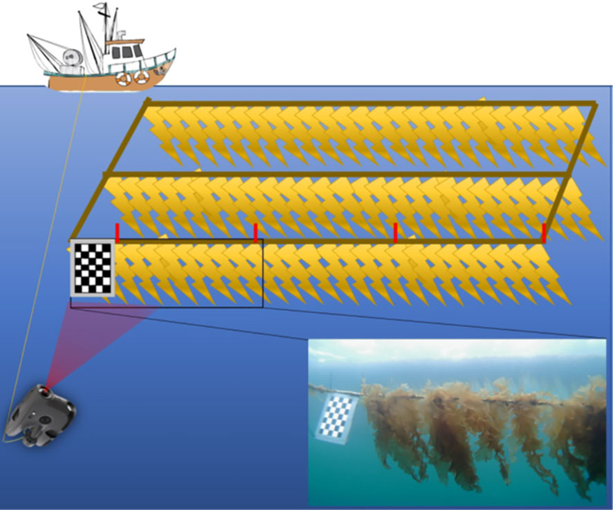
Figure 2 Schematic of the image sampling method, where a checkerboard was placed at the edge of the long line and used for size reference. Plastic cable ties indicated 1-meter replicates of kelp samples. A mini-ROV with internal RGB camera was used to collect videos along the longline.

After video recording, sporophytes of S. latissima from each 1 m replicate were sampled for wet weight biomass (presented as field-measured weight per meter) and length measurements (field-measured lamina + stipe + holdfast length, herein referred as lamina length) for validation. For the field-measured weight, the whole wet weight biomass of the 1 m cultivation line was considered. For field-measured length, 10 randomly selected S. latissima sporophyte specimens from each 1-meter replicate line were measured for lamina, as well as lamina width at the widest point. Only 10 sporophytes within each 1-meter replicate were chosen because it would be too time consuming to measure the length of each individual specimen (densities can reach many hundreds of individuals per meter). This is also a common methodology used by seaweed farmers when carrying out field monitoring. The same method was repeated on each field day, meaning that the sampling is destructive – the seaweed was permanently removed from the cultivation line for biomass and length measurements.

To investigate the influence of environmental variables, such as particles (phytoplankton and detritus), irradiance and wind speed, on water visibility and image quality for post-processing, additional environmental data were collected. A submersible fluorometer sensor (C3, Turner Designs, USA) was attached at the edge of the farm and placed at 3 m depth (Figure 1C). The sensor measured temperature (°C), chlorophyll a fluorescence (calibrated later to concentration [Chl a] in mg m^-3) and turbidity (Relative Fluorescence Unit - calibrated later to Formazin Turbidity Unit (FTU)) every 10 minutes from mid-February to mid-June. The C3 submersible was also equipped with an antifouling copper plate and a mechanical wiper that rotates and cleans the optical sensor before each measurement (every 10 min). Data on wind speed (m s^-1) from February until mid-June was obtained hourly from Sula meteorological station (located west of Frøya, Figure 1) and retrieved from the Norwegian Weather Service Center (https://seklima.met.no/).

2.2 Image processing

2.2.1 ImageJ-derived measurements

To ascertain whether reliable measurements (in this case length) were possible using underwater imaging, preliminary estimates derived from the image frames were compared to the manual measurements obtained from the kelp harvested in the field. For that, comparisons were made between the average length of randomly selected “imaged” fronds (see more below) and the average length of 10 harvested fronds measured in the field (explained in section 2.1). The reason we decided to do this initial step was to ascertain whether, on average, sporophyte length measured manually from an underwater image had comparable results with manual measurements in the field before applying CV (OpenCV package in python) techniques. To achieve this, image frames that included the checkerboard for scaling were selected and uploaded to ImageJ (Image Processing and Analysis in Java) (Figure 3). The checkerboard in the frame was used as a size reference to set a scale for the number of pixels per centimetre (pixels cm^-1) for the corresponding frame (Figure 3). Then, 10 kelp specimens in each frame were randomly selected, and their length in centimetres (cm) were measured by drawing a line from the tip to the holdfast of the specimen, using the “line” and “measure” tools in ImageJ (Figure 3). A total of 6 frames for each 1-meter replicate were selected based on checkerboard visibility, and with different distances and positions of the kelp. It was decided that 6 frames were sufficiently representative to capture some variability in the image data, while also being manageable for manual processing. For each frame, 10 sporophyte lengths were measured accounting for a total of 60 measurements per day (10 sporophytes × 6 frames). The pipeline was repeated using image data from each field day (10 sporophytes × 6 frames × 7 sampling days).

Figure 3

Figure 3 Pipeline for manual annotation of length performed using ImageJ. Extraction of image frames from videos. Using a checkerboard to set scale of pixels per centimetre (pixels cm^-1). Drawing and measuring length from tip to holdfast (indicated by yellow lines) of ten randomly selected kelp specimens.

2.2.2 Open CV-derived measurements

Kelp area estimates from 1-meter replicates were performed using the Python library OpenCV. The pipeline started with extraction of six frames of the first kelp replicate from the video collected by the mini-ROV camera (Figure 4). The six frames selected were the same frames used for the ImageJ-derived estimates. The region of interest (ROI) in the frame, defined as the width of the 1-meter replicate and height, was cropped from the original frame to sufficiently capture the full length of the kelp within 1-meter replicate (Figure 4).

Figure 4

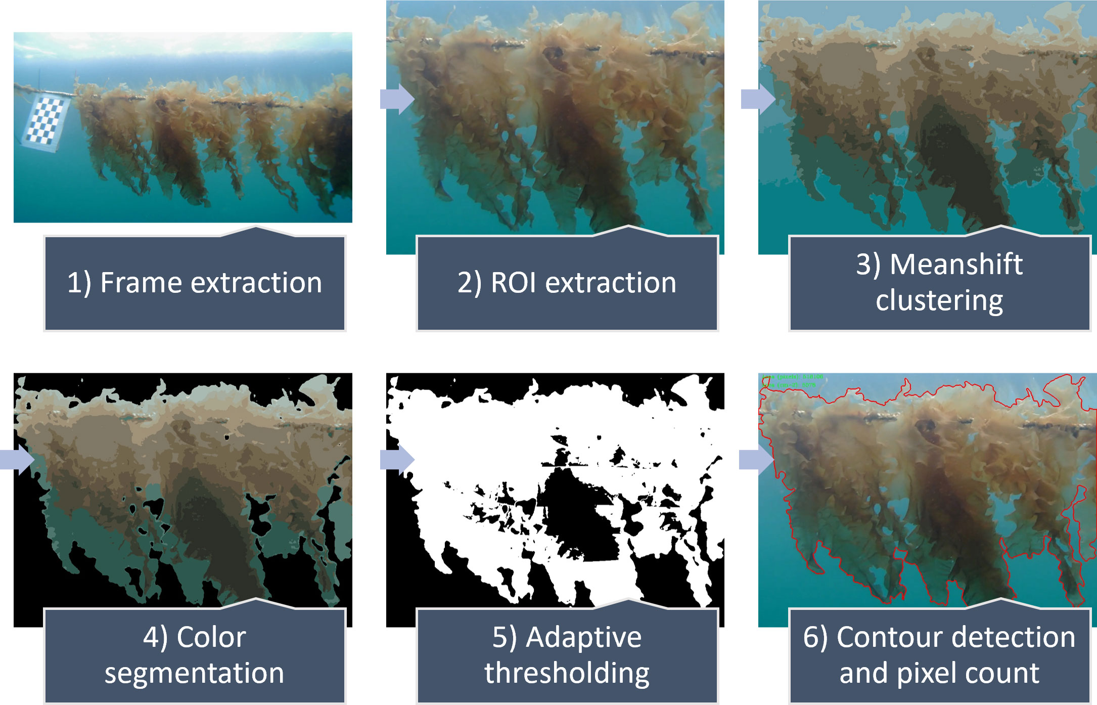
Figure 4 Pipeline for the computer vision (CV) area estimation performed with OpenCV. Extraction of frames from image data. Extraction of region of interest (ROI) from frame. Mean shift clustering of pixel values. Segmentation of object of interest (OOI) based on colour. Masking out OOI from the background using adaptive thresholding. Detection of the contour of the OOI and counting of area pixels, converted to square decimetres (dm² m^-1) using known pixel width and real-world width (one meter) of the frame as size reference, resulting in CV-derived area.

Before segmenting the kelp from the images, a type of unsupervised learning algorithm known as ‘mean shift clustering’ was applied to distinguish foreground kelp, background and sea water as separate features. First introduced by Fukunaga and Hostetler (1975) and reintroduced by Comaniciu and Meer (2002) as a general-purpose algorithm for image segmentation and filtering, the algorithm used here deconstructs the original image into several homogeneous, unstructured segments based on the similarity of colour space representation of neighbouring pixels (Figure 4). Colour segmentation was then applied to distinguish the kelp as the object of interest (OOI) from the surrounding background in the frame (Figure 4). Next, adaptive thresholding (Yang et al., 1994) was applied to mask out the OOI from the background, allowing detection of the contour of the OOI (Figure 4). Lastly, the number of individual pixels in the contour area was counted. The pixel count was converted to square decimetres (dm² m^-1) by using the 1-meter width of the ROI as a scale and is defined herein as CV-derived area per meter. The pipeline was repeated using image data from each field day.

2.3 Statistical analyses

Statistical analyses were performed using NumPy, SciPy, scikit-learn and Matplotlib, libraries for data analysis and visualization in Python and Matlab. Relationships between field-measured length and weight versus ImageJ length and CV-derived area were investigated by applying regressions and evaluated by their coefficient of determination (r²).

3 Results

3.1 Environmental parameters

Average wind speed varied from February until mid-June, reflecting the dynamic weather in the Frøya region, and was particularly strong (up to 20 m s^-1) during March and early April (Figure 5A). Weakening of wind speed (< 10 m s^-1) observed from mid- to late April likely contributed to the shoaling of the mixing layer depth and phytoplankton bloom formation. Environmental variables, such as Chl a and turbidity levels varied during the field season (Figure 5B). Several peaks in [Chl a] were observed from February to June (5b), with a short peak in late March (~2.5 mg m^-3), a long peak around mid-April (up to 5.7 mg m^-3) and variable values from late May until mid-June (< 4 mg m^-3). The overall trend was towards higher concentrations in the second half of the field campaign. The [Chl a] served as a proxy for phytoplankton biomass and, thus, indicated when phytoplankton blooms ([Chl a] >~ 3 mg m^-3) occurred. Turbidity showed significant variability throughout the field season (Figure 5B). A relatively similar trend compared to [Chl a] until late May was observed, with a long peak in turbidity levels in mid-to-late April (> 0.2 FTU). A short turbidity peak was observed in mid-June (> 0.2 FTU) (Figure 5B). Seawater temperature showed a gradual increase from February until the end of June, varying from 5.6°C to 9.4°C (Figure 5C).

Figure 5

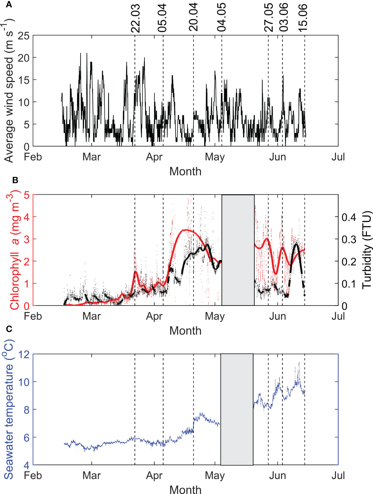
Figure 5 (A) Average wind speed (m s^-1) at Sula meteorological station, and (B) chlorophyll a concentrations (red, mg m^-3) and turbidity (black, FTU) and (C) seawater temperature (°C) at Måsskjæra farm from February 16^th to June 15^th, 2022. Lines indicate the sampling dates.

3.2 Image quality

Differences in the image quality of the videos/frames used for processing were observed between different sampling days (Figure 6). For example, early in the season (22^nd March and 5^th April), the image quality was very high, indicating good water visibility. During the period of the spring phytoplankton bloom (first peak 20^th April, later peaks on May 27^th and June 3^rd), the observed image quality decreased, indicating bad water visibility due to particles present in the water and the absorption of light from phytoplankton. The visibility of the images slightly improved on May 4^th (a period between phytoplankton bloom peaks). On the last sampling day, June 15^th, the observed image quality was poor, coinciding with a high concentration of phytoplankton and other particles (indicated by a high peak in Chl a and turbidity concentrations Figure 5B). Image quality due to poor visibility decreased towards the end of the cultivation period due to the high abundance of phytoplankton and other particles in the water.

Figure 6

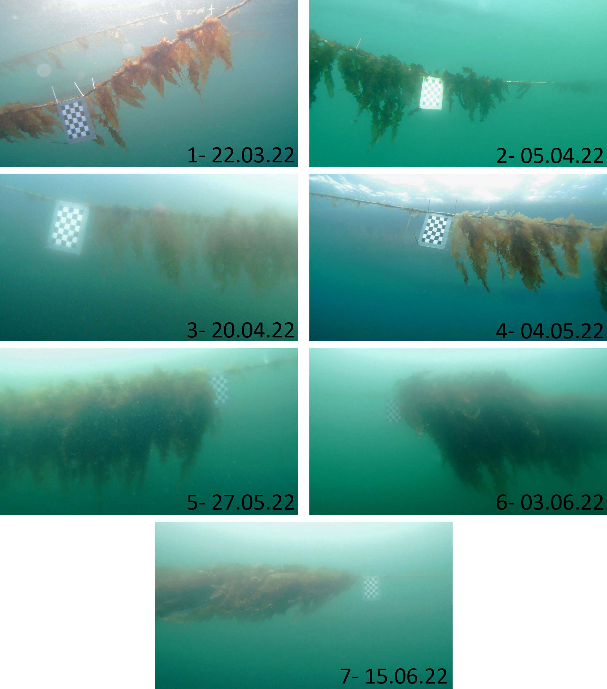
Figure 6 Example of image frames collected during each sampling day. Note the variability in water colour, clarity, and the positioning of the kelp (vertical or diagonal) in the cultivation line.

3.3 Calibration and validation

Field-measured verification of kelp length and biomass had a positive power relationship (r² = 0.941, biomass = 5.197e-06 length^3.037, p<0.05) (Figure 7A). On June 15 (latest day in the season), sporophytes were smaller (average= 65.9 cm) than specimens from late May and early June (> 80 cm in May 27^th and June 3^rd) (Figure 7A). Similarly, imageJ-derived length estimations had a positive strong correlation with field-measured biomass (r² = 0.977, biomass = 3.713e-06 ImageJ-length^3.083, p<0.05) (Supplementary Figure S1, Supplementary Material). The relationship between length (field-measured and derived from ImageJ) and biomass is best approximated by an isometric function (exponent b=3).

Figure 7

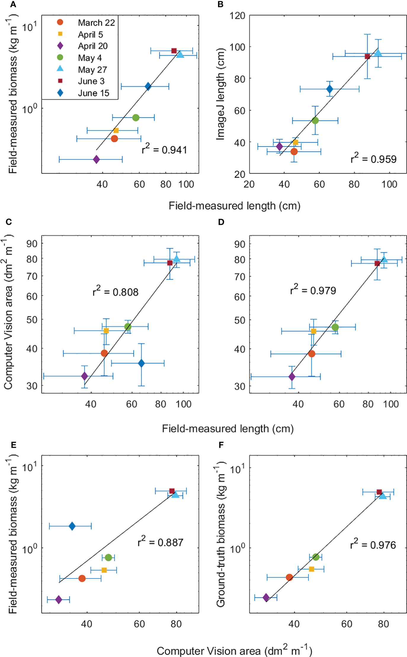
Figure 7 Relationships between S. latissima (A) field-measured lamina length (cm) and field-measured wet weight (kg m^-1), (B) field-measured length (cm) and ImageJ-derived length (cm), (C) field-measured length (cm) and computer vision (CV)-derived area per meter (dm² m^-1) with and (D) without the outlier (June 15^th), (E) CV-derived area per meter (dm² m^-1) and field-measured wet weight (kg m^-1) with and (F) without the outlier (June 15^th). Error bars show the standard deviation of ground-truth length (n=10 sporophytes in 1-meter line), ground-truth weight (n=1 in triplicate 1-meter line), ImageJ length (n=6 image frames, 10 sporophyte per frame in 1-meter line).

ImageJ-derived length (ranging from 33.9 cm to 95.7 cm) had a positive correlation with field-measured length (ranging from 37.4 cm to 93.5 cm) for the 10 randomly selected sporophytes (images and field measurements) (r² = 0.959, ImageJ-length = 1.208 field-measured length – 13.817, p < 0.05, Figure 7B). Variability was larger in field-measured length (standard deviation ranged from 12.4 cm to 19.5 cm) compared to variability from ImageJ-derived measurements (standard deviation ranging from 2.8 cm to 14.0 cm) (Figure 7B).

A strong positive power relationship (r² = 0.808, CV area = 0.7327 length^1.026, p < 0.05) was observed between field-measured length and image CV-derived kelp area (Figure 7C). Both CV-derived area and field-measured length showed large variation between sampling timepoints. CV-derived area ranged from 32.2 dm² m^-1 to 79.3 dm² m^-1 (Figure 7C). Measurements from the last sampling day (June 15^th) had CV-derived area (35.6 dm² m^-1) notably below the power trend. When removing the June 15^th data from the analysis, an even stronger significant power relationship (r² = 0.979, CV area = 0.988 length^0.9694, p <0.01) was observed (Figure 7D). The area-length relationship with an exponent being equal to 1 indicates a linear relationship between these two variables, where the increase in area is directly proportional to the increase in length.

A wide range in field-measured weight was observed between sampling timepoints, ranging from 0.24 kg to 4.97 kg per meter (Figure 7E). When comparing area measurements (CV-derived) with biomass (wet weight), a strong positive power relationship was observed (biomass = 2.204e-05 CV area^2.81, r² =0.887) (Figure 7E). Similar to the relationship between CV-derived area and field-measured length, measurements from June 15^th had a lower CV-derived area (35.6 dm² m^-1) compared to the trend, and if removed, the relationship becomes stronger (r² = 0.976, biomass = 1.231e-06 CV area^3.472, p < 0.01) (Figure 7F).

4 Discussion

4.1 Effect of environmental factors on image quality

The image quality varied widely in this study as a function of the inherent optical properties (IOPs) of the water, including coloured dissolved organic matter (CDOM) and particle concentrations, such as phytoplankton and detritus. The IOPs, such as phytoplankton cells (light absorption and scattering), non-algal particles (NAP, e.g. detritus and sediments, mainly light scattering) and CDOM (absorbing), will tend to absorb (through pigments) or scatter light through deflection (Werdell et al., 2018), reducing the amount of light reflected from the kelp to the camera. The influence of IOPs varies with the water type and depends on where the seaweed is cultivated, making underwater imaging more suitable for clear, open offshore waters (Broch et al., 2019) and more challenging in turbid and brackish coastal seawater.

Besides IOPs, the apparent optical properties (AOPs) of the water, meaning the angular distribution and intensity of the ambient light-field, can also impact the quality of the images taken under natural light conditions (Johnsen et al., 2009). Measurements of underwater light conditions were not conducted in our study; however, according to our observations, the ambient irradiance impacted water quality image. In this study, incident light would, in some cases, improve water column visibility and detection of kelp from the surrounding water, while in other cases, it could overexpose the images, reducing contrast and corresponding loss of colour information. Kelp self-shading from incident light, which was more prominent as the kelp became bigger, impacted negatively the algorithms for area detection, particularly towards the later stages of the cultivated kelp (early summer). Kjerstad (2014) showed that light attenuation between the camera and the object limits the range at which pictures of organisms can be taken, since spatial and colour (spectral) resolution becomes distorted in underwater images as the distance to an OOI increases. Artificial light might be a solution, although, in waters with a lot of particles (plankton, sediments and marine snow/detritus), direct light can intensively illuminate those particles, creating bright spots of scattered light and causing image degradation (Boffety and Galland, 2012). Choice of camera, field of view, spectral resolution and positioning of the external light sources are important pre-image processing factors that should be considered before video recording, in order to optimize post-processing time and image quality.

Waters around Frøya are known to be highly productive, where phytoplankton blooms can start from late March and persist until June-July (Fragoso et al., 2021). Moreover, CDOM concentrations are known to increase from spring and peak in summer as freshwater input from rivers is accumulated in the NCC, the main current along the coastal of Norway (Nima et al., 2016). In this study, CDOM was not measured; however, the other IOPs, such as [Chl a] for a proxy of phytoplankton biomass and turbidity, for particle concentration, clearly impacted the quality of the image. The combination of high turbidity and [Chl a]- suggesting not only that a bloom is occurring but that it is composed of large cells, colonies and aggregates - makes the water visibility worse, particularly in mid-June. Such conditions become even more detrimental as the kelp gets bigger and the camera needs to move further away to increase the FOV, allowing light to be more attenuated between the camera and the OOI. Chain-forming diatom blooms dominated by the genera Chaetoceros, Skeletonema and Thalassiosira are common during spring in Frøya (Fragoso et al., 2019, Fragoso et al., 2021), as well as many other coastal northern regions (Throndsen et al., 2007), making visibility a challenge for ROV video recording at seaweed farms. Water quality improved on 4^th May, after the decline of the first bloom and potentially because of a storm that diluted the particle density throughout the mixed layer depth. Marine snow, as well as zooplankton abundance, which are high in Frøya waters (Fragoso et al., 2019) and other coastal productive regions of Norway, would increase the turbidity signal after bloom conditions, being an additional challenge for water visibility and kelp size inspection.

Underwater imaging enhancement (UIE), such as white balance, dehazing algorithms and histogram equalization are modern tools to improve the contrast of objects from ocean RGB imagery, allowing more accurate segmentation and identification of the OOI (Mathur and Goel, 2022). Mohamed et al. (2020) used the Multi-Scale Retinex (MSR) algorithm for image correction and the YOLO algorithm to enhance fish detection and tracking in tanks, increasing underwater detection of fish specimens by three times. UIE in seaweed and fish farms could be a potential tool to reduce the optical effects of particles in the water, improving the accuracy of our model, particularly for conditions later in the season due to increased turbidity. Another possibility could be to monitor phytoplankton concentrations and turbidity levels using sensors at the kelp farm and adapt the time of video recording to periods with lower turbidity levels and between phytoplankton blooms, in order to collect higher quality imagery.

Strong currents were also another issue that impacted the quality of data. In our studies, slack tides (particularly low tide) were the best periods to video record the kelp lamina hanging vertically from the ropes. This allowed the best positioning of the kelp to be able to better extract area information. According to most of our images, the kelp was aligned vertically from the cultivation rope, except for June 15^th, which contributed to the lower rendering of CV-derived area estimations. This suggests that the environmental conditions, possibly obtained from instruments such as acoustic doppler current profilers (ADCPs) and optical instruments for IOPs measurements, need to be taken into consideration before underwater video recording/digital imaging. Awareness of the impact of environmental variables on the reliability of remote sensing results (e.g. seagrass beds, Nahirnick et al. (2019)) has been raised and similar approaches could be implemented for seaweed farms. Pre-analyses of the environmental conditions (irradiance, turbidity and current velocities) from sensors attached to kelp farm infrastructure can help improve decisions about the optimum conditions for underwater farm inspection (Bell et al., 2020).

4.2 Kelp length and area estimations from underwater RGB imagery

Our work indicates that it is possible to detect and derive kelp size from RGB camera images. Through human supervision, length measurements of 10 randomly selected sporophytes extracted from the frames using imageJ (Figure 3) demonstrated strong relationships with measurements done by hand in the field (also 10 randomly selected sporophytes from 1m of cultivation line). Variability in the data is likely related to the fact that these two 1m sections (for image and field measurements) were not the same. Human annotation of traits (length, area, point count, segmentation) is a useful tool in underwater biological image analysis (Gomes-Pereira et al., 2016), which, when combined with CV, has the potential to simplify in situ size estimation of underwater organisms.

Automated size estimation, as well as species identification and animal tracking, via CV techniques, are modern tools in ecology. Estimation of individual biomass of marine organism from dimensions derived from images is possible because of the strong isometric/allometric biomass-size relationships expected in many organisms, including macroalgae and seagrasses (Scrosati, 2006; Scrosati et al., 2020). In S. latissima, allometric models (where the organism does not maintain its shape as it grows) have been shown to explain a substantial portion of thallus fresh weight (Campbell and Starko, 2021). However, these relationships have previously been studied in individual specimens. In our study, kelp area and biomass estimations were retrieved from a 1-meter line (rather than individuals), while lengths were retrieved from individuals. This makes it complicated to compare our results to these growth models, and it is the reason that we do not observe an isometric/allometric growth function when comparing individual lengths to CV-derived area. Despite this, we observed an isometric relationship between average lamina length and total biomass within 1m line, suggesting that the “canopy” maintains its shape as it grows (conceptually, it can perhaps be thought of as an expanding “cylinder”, horizontally oriented in the water column).

Our findings indicate that it is likely possible to derive robust size information about kelp by applying CV techniques to underwater RGB imagery. This technique is commonly applied in agriculture and aquaculture. For example, above ground biomass has been successfully estimated in wheat crops using airborne laser scanning for 3D point cloud reconstruction when comparing estimated volume and ground-truth biomass (Walter et al., 2018). The plant height of summer barley has also been suggested as a good proxy for fresh and dry biomass using an RGB camera on a small unmanned aerial vehicle (UAV) (Bendig et al., 2015). Comparisons between seaweed biomass and area coverage from intertidal zones derived from UAV multispectral images revealed a positive correlation (r^2 = 0.8, 0.73 and 0.59, respectively for Ulva pertusa, Sargassum thunbergii and Sargassum fusiforme), although accuracy decreased in highly dense beds due to mutual masking of seaweed (Chen et al., 2022). For fish farm applications, CV-derived image area of grey mullet, carp and St. Peter’s fish were well correlated to mass (r^2 = 0.954, 0.986, 0.986, respectively) (Zion et al., 1999), while shape and weight exhibited only a 3% error rate in prediction accuracy with machine learning algorithms (Odone et al., 2001). Side view imaging (2D CV) of Scortum barcoo showed that shape is a good predictor (r^2 = 0.99) for measuring fish weight outside tanks (Viazzi et al., 2015). The fact that area estimates showed a positive relationship with length and weight in our studies indicates the feasibility of using area as a proxy for biomass under suitable conditions (vertically aligned kelp). Consequently, our results indicate that a model using area estimates as a proxy for biomass can be further developed and eventually applied to accurately predict kelp biomass in situ throughout the cultivation season.

These predictions will likely become even more common as machine learning techniques improve and become more mainstream (Weinstein, 2018). During the last decade, machine/deep learning techniques have been increasingly applied to classify distinct functional groups/species in macroalgae and aquatic vegetation (e.g. seagrass beds) from remote sensing imaging derived from drones (Duffy et al., 2018; Chen et al., 2022; Tahara et al., 2022). For seaweed cultivation, however, emerging technologies and methodologies for remote sensing and precision farming, are in their infancy, although they show great promise. Bell et al. (2020), for instance, used underwater colour images from mini-ROVs and side scan sonar of kelp farm longlines, combined with deep learning models, to classify juvenile kelp from the images and acoustic returns before and after pneumatocyst (gas bladders) formation. These acoustic approaches can be a potential way to quantify biomass in species with gas bladders since total gas volume from pneumatocyst increases as kelp laminas grow (Bell et al., 2020). Stenius et al. (2022) also explored the use of side-scan sonar for detection of ropes and buoys at a kelp farm, which could be successfully implemented for biomass estimations of seaweed that possesses pneumatocysts. However, it is unclear whether this methodology would be as successful for other cultivated kelp species that lack pneumatocysts. From RGB imagery, machine learning algorithms successfully classified kelp underwater background, in spite of water motion, although these authors emphasized that water clarity is a requirement for the best visibility and suitability of the model (Bell et al., 2020).

In this study, we showed that a robust relationship between CV-derived area and ground-truth biomass and length. However, post-processing segmentation was time consuming, since we had to manually tune the algorithms for distinct environmental conditions (low versus high turbidity, changes in irradiance, colour hue and contrasts, etc). By combining similar detection algorithms developed by Bell et al. (2020) and others (Duffy et al., 2018; Chen et al., 2022), with the methodology developed in our study, further segmentation for kelp density and automated kelp area estimation for biomass prediction could be feasible. For maintaining the simplicity of this method, density effects (i.e. sporophytes per m) on biomass were not considered and quantified. CV-derived area, by its nature, should capture density more effectively than image derived length. The nature of this relationship (biomass-density) should be explored in detail, however, to verify if cultivation lines with very high densities are likely to have their biomass underestimated due to the inability to capture the third growth dimension (essentially the “thickness” or “bushiness” of the canopy). The relationship between biomass and density, however, is not simplistic as phenomena such as “self-thinning” at high densities, and intra-specific “dynamic thinning” in response to abiotic factors, can occur (see review by Scrosati (2005)).

In order to upscale this method, larger sample datasets can be used as calibration and validation data, as to reduce the statistical uncertainty and provide cross-validation of the results (Bendig et al., 2015). The ultimate goal would be an universally applicable model for different kelp species. However, it is possible that location-specific models will be required. Campbell and Starko (2021) demonstrated that allometric models, for predicting thallus weight from length, were broadly applicable at sites with similar environmental conditions, but suggested the need for region-specific models between substantially different locations. It should be examined if this finding holds true for estimating biomass on cultivation lines from canopy area. If region-specific models need to be constructed, that would still likely be worth the relatively small time invested by the farmer(s) in order to later automate the process of biomass estimation from images.

4.3 Future perspectives for biomass estimation of cultivated kelp

The use of mini-ROVs has been applied in many studies for short-distance inspection and monitoring of several habitats, including benthos (Nevstad, 2022), kelp forests (Summers et al., 2022) and coral reefs (Raoult et al., 2020). In this study we demonstrate that the use of a mini-ROV, equipped with an RGB camera, can reliably estimate kelp biomass using underwater imaging and CV techniques.

Our preliminary results focused on a small section of a farm, which is most likely not representative of the whole farm and has considerable constraints, such as the need for human operation, limited battery time and tether length (Sørensen et al., 2020). Consequently, the use of the ROV can only be applied in sub-sections of the farm to give an idea of how heterogeneously seaweed grow in space and time. In this study we tested our method at the edge of the farm for simplicity (accessibility and so as not to interfere with farm operations). Performing this task inside the farm (e.g. between cultivation lines) is likely to raise issues relating to maneuverability within confined spaces. For further estimations at a “whole farm” scale, other types of observation platforms equipped with cameras and additional sensors could be used, but this will likely depend on the exact farm design and location (e.g. vertical or horizontal cultivation lines, inshore or offshore, low or high energy environment). As farms scale up in size, there will be an increasing need for kelp farm monitoring at different scales, and combinations of platforms, such as satellites (Jin et al., 2023), UAVs (Bell et al., 2020), AUVs (Stenius et al., 2022) and ROVs.

Here, we anticipate that our concept can be used as the foundation to upscale imagery as a reliable tool for biomass estimation of kelp. For example, Stenius et al. (2022) developed a methodology where they deployed an AUV to monitor a whole kelp-farm autonomously and continuously. In their small-scale scheme, an AUV followed pre-programmed or self-detected sampling patterns based on the outline of the farm and, thus, enabled high resolution monitoring of an entire kelp-farm throughout the cultivation season. Other possibilities could be moving the cameras along strategically structured cables throughout the farm, removing the need for underwater vehicles. Perhaps the cameras do not need to move around at all, but rather placed in fixed positions where they can capture enough image data to build up a representative picture of the total farmed kelp biomass. Ultimately, the goal of the technology and method should be to optimize accuracy of biomass estimation, providing sufficient monitoring, while at the same time minimizing operational risks and costs.

5 Conclusion

Our proof-of-concept results indicate that CV-derived area estimation can serve as a robust proxy for biomass estimation of cultivated kelp. However, accuracy of the data is strongly related to the visibility of the water and current speed. Although there was still a strong relationship when water visibility was reduced, the relationship improved when outliers (with poor water visibility) were removed.

As technology advances and machine learning algorithms for object detection improve, kelp biomass estimation in situ with camera systems, perhaps combined with other methods (e.g. acoustics), can be a viable option for large scale farm monitoring. We see this work as an important step towards that goal, where we also envisage autonomous data collection and real-time processing.

Data availability statement

The datasets (source code) presented in this study can be found in the following repository: https://github.com/monitare.

Author contributions

MO: Data curation, Formal analysis, Investigation, Methodology, Validation, Visualization, Writing – original draft, Writing – review & editing. PT: Data curation, Formal analysis, Investigation, Methodology, Software, Supervision, Validation, Visualization, Writing – review & editing. DA: Supervision, Conceptualization, Writing – review & editing. GJ: Resources, Supervision, Writing – review & editing. GF: Conceptualization, Funding acquisition, Project administration, Resources, Supervision, Visualization, Writing – original draft, Writing – review & editing.

Funding

The author(s) declare that financial support was received for the research, authorship, and/or publication of this article. This work was supported by the Research Council of Norway (RCN) through the following project: “Autonomous underwater monitoring of kelp-farm biomass, growth, health and biofouling using optical sensors”, MoniTARE (315514). GJ received funding RCN 223254 grant (Center of Excellence, Autonomous Marine Operations and Systems, AMOS).

Acknowledgments

We would like to thank Seaweed Solutions (SES) for providing access to their kelp farm, the irradiance data, in addition to the assistance of SES employees and resources for collection of water samples. Data from this manuscript is part of a NTNU Master’s thesis (Overrein, 2023) and is available online (https://ntnuopen.ntnu.no/ntnu-xmlui/handle/11250/3086275). We would also like to thank the journal editor and two reviewers of this paper for their constructive feedback which has strengthened the quality of this manuscript.

Conflict of interest

The authors declare that the research was conducted in the absence of any commercial or financial relationships that could be construed as a potential conflict of interest.

Publisher’s note

All claims expressed in this article are solely those of the authors and do not necessarily represent those of their affiliated organizations, or those of the publisher, the editors and the reviewers. Any product that may be evaluated in this article, or claim that may be made by its manufacturer, is not guaranteed or endorsed by the publisher.

Supplementary material

The Supplementary Material for this article can be found online at: https://www.frontiersin.org/articles/10.3389/fmars.2024.1324075/full#supplementary-material

References

Albrecht M. (2023). A Norwegian seaweed utopia? Governmental narratives of coastal communities, upscaling, and the industrial conquering of ocean spaces. Marit. Stud. 22, 37. doi: 10.1007/s40152-023-00324-2

CrossRef Full Text | Google Scholar

Alleway H. K. (2023). Climate benefits of seaweed farming. Nat. Sustain. 6, 356–357. doi: 10.1038/s41893-022-01044-x

CrossRef Full Text | Google Scholar

Bell T. W., Nidzieko N. J., Siegel D. A., Miller R. J., Cavanaugh K. C., Nelson N. B., et al. (2020). The utility of satellites and autonomous remote sensing platforms for monitoring offshore aquaculture farms: A case study for canopy forming kelps. Front. Mar. Sci. 7. doi: 10.3389/fmars.2020.520223

CrossRef Full Text | Google Scholar

Bendig J., Yu K., Aasen H., Bolten A., Bennertz S., Broscheit J., et al. (2015). Combining UAV-based plant height from crop surface models, visible, and near infrared vegetation indices for biomass monitoring in barley. Int. J. Appl. Earth Obs. Geoinf. 39, 79–87. doi: 10.1016/j.jag.2015.02.012

CrossRef Full Text | Google Scholar

Bewley M. S., Douillard B., Nourani-Vatani N., Friedman A., Pizarro O., Williams S. B. (2012). Automated species detection: an experimental approach to kelp detection from sea-floor AUV images. In Proc Australas Conf Rob Autom. 2012.

Google Scholar

Boffety M., Galland F. (2012). Phenomenological marine snow model for optical underwater image simulation: Applications to color restoration. 2012 Oceans - Yeosu (IEEE) 1–6. doi: 10.1109/OCEANS-Yeosu.2012.6263448

CrossRef Full Text | Google Scholar

Broch O. J., Alver M. O., Bekkby T., Gundersen H., Forbord S., Handå A., et al. (2019). The kelp cultivation potential in coastal and offshore regions of Norway. Front. Mar. Sci. 5. doi: 10.3389/fmars.2018.00529

CrossRef Full Text | Google Scholar

Broch O. J., Daae R. L., Ellingsen I. H., Nepstad R., Bendiksen E.Å., Reed J. L., et al. (2017). Spatiotemporal dispersal and deposition of fish farm wastes: A model study from central Norway. Front. Mar. Sci. 4. doi: 10.3389/fmars.2017.00199

CrossRef Full Text | Google Scholar

Campbell J., Starko S. (2021). Allometric models effectively predict Saccharina latissima (Laminariales, Phaeophyceae) fresh weight at local scales. J. Appl. Phycol. 33, 491–500. doi: 10.1007/s10811-020-02315-w

CrossRef Full Text | Google Scholar

Chen J., Li X., Wang K., Zhang S., Li J. (2022). Estimation of seaweed biomass based on multispectral UAV in the intertidal zone of Gouqi Island. Remote Sens. 14 (9), 2143. doi: 10.3390/rs14092143

CrossRef Full Text | Google Scholar

Comaniciu D., Meer P. (2002). Mean shift: a robust approach toward feature space analysis. IEEE Trans. Pattern Anal. Mach. Intell. 24, 603–619. doi: 10.1109/34.1000236

CrossRef Full Text | Google Scholar

Duarte C. M., Bruhn A., Krause-Jensen D. (2021). A seaweed aquaculture imperative to meet global sustainability targets. Nat. Sustain. 5, 185–193. doi: 10.1038/s41893-021-00773-9

CrossRef Full Text | Google Scholar

Duffy J. P., Pratt L., Anderson K., Land P. E., Shutler J. D. (2018). Spatial assessment of intertidal seagrass meadows using optical imaging systems and a lightweight drone. Estuar. Coast. Shelf Sci. 200, 169–180. doi: 10.1016/j.ecss.2017.11.001

CrossRef Full Text | Google Scholar

Ervik H., Finne T. E., Jenssen B. M. (2018). Toxic and essential elements in seafood from Mausund, Norway. Environ. Sci. Pollut. Res. 25, 7409–7417. doi: 10.1007/s11356-017-1000-4

CrossRef Full Text | Google Scholar

Fischell E. M., Gomez-ibanez D., Lavery A., Stanton T., Kukulya A. (2019). Autonomous underwater vehicle perception of infrastructure and growth for aquaculture. IEEE ICRA Workshop Underwater Robotic Percept. 2019, 1–7.

Google Scholar

Førde H., Forbord S., Handå A., Fossberg J., Arff J., Johnsen G., et al. (2016). Development of bryozoan fouling on cultivated kelp (Saccharina latissima) in Norway. J. Appl. Phycol. 28, 1225–1234. doi: 10.1007/s10811-015-0606-5

CrossRef Full Text | Google Scholar

Fragoso G. M., Davies E. J., Ellingsen I., Chauton M. S., Fossum T., Ludvigsen M., et al. (2019). Physical controls on phytoplankton size structure, photophysiology and suspended particles in a Norwegian biological hotspot. Prog. Oceanogr. 175, 284–299. doi: 10.1016/j.pocean.2019.05.001

CrossRef Full Text | Google Scholar

Fragoso G. M., Johnsen G., Chauton M. S., Cottier F., Ellingsen I. (2021). Phytoplankton community succession and dynamics using optical approaches. Cont. Shelf Res. 213, 104322. doi: 10.1016/j.csr.2020.104322

CrossRef Full Text | Google Scholar

Fukunaga K., Hostetler L. (1975). The estimation of the gradient of a density function, with applications in pattern recognition. IEEE Trans. Inf. Theory 21, 32–40. doi: 10.1109/TIT.1975.1055330

CrossRef Full Text | Google Scholar

Gomes-Pereira J. N., Auger V., Beisiegel K., Benjamin R., Bergmann M., Bowden D., et al. (2016). Current and future trends in marine image annotation software. Prog. Oceanogr. 149, 106–120. doi: 10.1016/j.pocean.2016.07.005

CrossRef Full Text | Google Scholar

Hossain M. S., Sharifuzzaman S. M., Nobi M. N., Chowdhury M. S. N., Sarker S., Alamgir M., et al. (2021). Seaweeds farming for sustainable development goals and blue economy in Bangladesh. Mar. Policy 128, 104469. doi: 10.1016/j.marpol.2021.104469

CrossRef Full Text | Google Scholar

Hwang E. K., Yotsukura N., Pang S. J., Su L., Shan T. F. (2019). Seaweed breeding programs and progress in eastern Asian countries. Phycologia 58, 484–495. doi: 10.1080/00318884.2019.1639436

CrossRef Full Text | Google Scholar

Jin R., Ye Z., Chen S., Gu J., He J., Huang L., et al. (2023). Accurate mapping of seaweed farms with high-resolution imagery in China. Geocarto Int. 38 (1), 2203114. doi: 10.1080/10106049.2023.2203114

CrossRef Full Text | Google Scholar

Johnsen G., Volent Z., Sakshaug E., Sigernes F., Pettersson L. H., Kovacs K. (2009). "Remote sensing in the barents sea," in Ecosystem Barents Sea, eds. Sakshaug E., Johnsen G., Kovacs K.. (Trondheim: Tapir Academic Press), 630.

Google Scholar

Kjerstad I. (2014). Underwater Imaging and the effect of Inherent Optical Properties on image quality. [MSc thesis]. Norwegian University of Science and Technology.

Google Scholar

Mathur M., Goel N. (2022). Enhancement algorithm for high visibility of underwater images. IET Image Process. 16, 1067–1082. doi: 10.1049/ipr2.12210

CrossRef Full Text | Google Scholar

Mohamed H. E.-D., Fadl A., Anas O., Wageeh Y., ElMasry N., Nabil A., et al. (2020). MSR-YOLO: Method to enhance fish detection and tracking in fish farms. Proc. Comput. Sci. 170, 539–546. doi: 10.1016/j.procs.2020.03.123

CrossRef Full Text | Google Scholar

Nahirnick N. K., Reshitnyk L., Campbell M., Hessing-Lewis M., Costa M., Yakimishyn J., et al. (2019). Mapping with confidence; delineating seagrass habitats using Unoccupied Aerial Systems (UAS). Remote Sens. Ecol. Conserv. 5, 121–135. doi: 10.1002/rse2.98

CrossRef Full Text | Google Scholar

Nevstad M. B. (2022). Use of different imaging systems for ROV-based mapping of complex benthic habitats. [MSc thesis]. Norwegian University of Science and Technology.

Google Scholar

Nima C., Frette Ø., Hamre B., Erga S. R., Chen Y. C., Zhao L., et al. (2016). Absorption properties of high-latitude Norwegian coastal water: The impact of CDOM and particulate matter. Estuar. Coast. Shelf Sci. 178, 158–167. doi: 10.1016/j.ecss.2016.05.012

CrossRef Full Text | Google Scholar

Odone F., Trucco E., Verri A. (2001). A trainable system for grading fish from images. Appl. Artif. Intell. 15, 735–745. doi: 10.1080/088395101317018573

CrossRef Full Text | Google Scholar

Olafsen T., Winther U., Olsen Y., Skjermo J. (2012). "Value Creation Based on Productive Seas in 2050," in Norwegian: Verdiskapning basert på produktive hav i 2050. Det Kongelige Norske Videnskabers Selskab (DKNVS) and Norges Tekniske Vitenskapsakademi (NTVA).

Google Scholar

Overrein M. M. (2023). In situ biomass estimation of cultivated kelp using RGB imagery. [MSc thesis]. Norwegian University of Science and Technology.

Google Scholar

Raoult V., Tosetto L., Harvey C., Nelson T. M., Reed J., Parikh A., et al. (2020). Remotely operated vehicles as alternatives to snorkellers for video-based marine research. J. Exp. Mar. Bio. Ecol. 522, 151253. doi: 10.1016/j.jembe.2019.151253

CrossRef Full Text | Google Scholar

Scrosati R. (2005). Review of studies on biomass-density relationships (including self-thinning lines) in seaweeds: Main contributions and persisting misconceptions. Phycol. Res. 53, 224–233. doi: 10.1111/j.1440-1835.2005.tb00375.x

CrossRef Full Text | Google Scholar

Scrosati R. (2006). Length-biomass allometry in primary producers: Predominantly bidimensional seaweeds differ from the “universal” interspecific trend defined by microalgae Vasc. Plants. Can. J. Bot. 84, 1159–1166. doi: 10.1139/b06-077

CrossRef Full Text | Google Scholar

Scrosati R. A., MacDonald H. L., Córdova C. A., Casas G. N. (2020). Length and Biomass Data for Atlantic and Pacific Seaweeds From Both Hemispheres. Front. Mar. Sci. 7. doi: 10.3389/fmars.2020.592675

CrossRef Full Text | Google Scholar

Skagseth Ø., Drinkwater K. F., Terrile E. (2011). Wind- and buoyancy-induced transport of the Norwegian Coastal Current in the Barents Sea. J. Geophys. Res. 116, C08007. doi: 10.1029/2011JC006996

CrossRef Full Text | Google Scholar

Skjermo J., Aasen I. M., Arff J., Broch O. J., Carvajal A. K., Hartvig C. C., et al. (2014). A new Norwegian bioeconomy based on cultivation and processing of seaweeds: Opportunities and R&D needs. SINTEF. Available at: https://ntnuopen.ntnu.no/ntnu-xmlui/bitstream/handle/11250/2447684/A25981-++A+new+Norwegian+bioeconomy+based+on+cultivation+and+processing+of+seaweeds+%28ver.2%29-Jorunn+Skjermo.pdf?sequence=1.

Google Scholar

Sørensen A. J., Ludvigsen M., Norgren P., Ødegård Ø., Cottier F. (2020). “Sensor-Carrying Platforms.” in POLAR NIGHT Marine Ecology – Life and light in the dead of the night, eds Berge J., Johnsen G., Cohen J.. (Hampton Roads, VA, USA: OCEANS 2022) 380 pp. doi: 10.1007/978-3-030-33208-2

CrossRef Full Text | Google Scholar

Stenius I., Folkesson J., Bhat S., Sprague C. I., Ling L., Özkahraman Ö., et al. (2022). A system for autonomous seaweed farm inspection with an underwater robot. Sensors 22, 1–16. doi: 10.3390/s22135064

CrossRef Full Text | Google Scholar

Summers N., Berge J., Johnsen G., Mogstad A., Lovas H., Fragoso G. (2022). Underwater hyperspectral imaging of arctic macroalgal habitats during the polar night using a novel mini-ROV-UHI portable system. Remote Sens. 14 (6), 1325. doi: 10.3390/rs14061325

CrossRef Full Text | Google Scholar

Tahara S., Sudo K., Yamakita T., Nakaoka M. (2022). Species level mapping of a seagrass bed using an unmanned aerial vehicle and deep learning technique. PeerJ 10, e14017. doi: 10.7717/peerj.14017

PubMed Abstract | CrossRef Full Text | Google Scholar

Throndsen J., Hasle G. R., Tangen K. (2007). Phytoplankton of Norwegian coastal waters. (Almater Forlag AS).

Google Scholar

Tiller R. G., Hansen L., Richards R., Strand H. (2015). Work segmentation in the Norwegian salmon industry: The application of segmented labor market theory to work migrants on the island community of Frøya, Norway. Mar. Policy 51, 563–572. doi: 10.1016/j.marpol.2014.10.001

CrossRef Full Text | Google Scholar

van Dijk M., Morley T., Rau M. L., Saghai Y. (2021). A meta-analysis of projected global food demand and population at risk of hunger for the period 2010–2050. Nat. Food 2, 494–501. doi: 10.1038/s43016-021-00322-9

PubMed Abstract | CrossRef Full Text | Google Scholar

Viazzi S., Van Hoestenberghe S., Goddeeris B. M., Berckmans D. (2015). Automatic mass estimation of Jade perch Scortum barcoo by computer vision. Aquac. Eng. 64, 42–48. doi: 10.1016/j.aquaeng.2014.11.003

CrossRef Full Text | Google Scholar

Volent Z., Johnsen G., Sigernes F. (2007). Kelp forest mapping by use of airborne hyperspectral imager. J. Appl. Remote Sens. 1, 011503. doi: 10.1117/1.2822611

CrossRef Full Text | Google Scholar

Walter J., Edwards J., McDonald G., Kuchel H. (2018). Photogrammetry for the estimation of wheat biomass and harvest index. F. Crop Res. 216, 165–174. doi: 10.1016/j.fcr.2017.11.024

CrossRef Full Text | Google Scholar

Weinstein B. G. (2018). A computer vision for animal ecology. J. Anim. Ecol. 87, 533–545. doi: 10.1111/1365-2656.12780

PubMed Abstract | CrossRef Full Text | Google Scholar

Werdell P. J., McKinna L. I. W., Boss E., Ackleson S. G., Craig S. E., Gregg W. W., et al. (2018). An overview of approaches and challenges for retrieving marine inherent optical properties from ocean color remote sensing. Prog. Oceanogr. 160, 186–212. doi: 10.1016/j.pocean.2018.01.001

PubMed Abstract | CrossRef Full Text | Google Scholar

Yang J.-D., Chen Y.-S., Hsu W.-H. (1994). Adaptive thresholding algorithm and its hardware implementation. Pattern Recognit. Lett. 15, 141–150. doi: 10.1016/0167-8655(94)90043-4

CrossRef Full Text | Google Scholar

Zion B., Shklyar A., Karplus I. (1999). Sorting fish by computer vision. Comput. Electron. Agric. 23, 175–187. doi: 10.1016/S0168-1699(99)00030-7

CrossRef Full Text | Google Scholar

Zolich A., Faltynkova A., Johnsen G., Johansen T. A. (2022). Portable Catamaran Drone – an uncrewed sampling vehicle for micro-plastics and aquaculture research. (Hampton Roads, VA, USA: OCEANS 2022) 1–6. doi: 10.1109/OCEANS47191.2022.9977294

CrossRef Full Text | Google Scholar