DF-ParPINN: parallel PINN based on velocity potential field division and single time slice focus

Modified Benney-Luke equation (mBL equation) is a three-dimensional temporal-spatial equation with complex structures, that is a high-dimensional partial differential equation (PDE), it is also a new equation of the physical ocean field, and its solution is important for studying the internal wave-wave interaction of inclined seafloor. For conventional PDE solvers such as the pseudo-spectral method, it is difficult to solve mBL equation with both accuracy and speed. Physics-informed neural network (PINN) incorporates physical prior knowledge in deep neural networks, which can solve PDE with relative accuracy and speed. However, PINN is only suitable for solving low-dimensional PDE with simple structures, and not suitable for solving high-dimensional PDE with complex structures. This is mainly because high-dimensional PDEs usually have complex structures and high-order derivatives and are likely to be high-dimensional non-convex functions, and the high-dimensional non-convex optimization problem is an NP-hard problem, resulting in the PINN easily falling into inaccurate local optimal solutions when solving high-dimensional PDEs. Therefore, we improve the PINN for the characteristics of mBL equation and propose “DF-ParPINN: parallel PINN based on velocity potential field division and single time slice focus” to solve mBL equation with large amounts of data. DF-ParPINN consists of three modules: temporal-spatial division module of overall velocity potential field, data rational selection module of multiple time slices, and parallel computation module of high-velocity fields and low-velocity fields. The experimental results show that the solution time of DF-ParPINN is no more than 0.5s, and its accuracy is much higher than that of PINN, PIRNN, cPINN, and DeepONet. Moreover, the relative error of DF-ParPINN after deep training 1000000 epochs can be reduced to less than 0.1. The validity of DF-ParPINN proves that the improved PINN also can solve high dimensional PDE with complex structures and large amounts of data quickly and accurately, which is of great significance to the deep learning of the physical ocean field.

1 Introduction

With the rapid development of computer technology, scientific computation has become the third scientific method that can be juxtaposed with theory and experiments (Shi, 2001; Lu and Guan, 2004). Solving various partial differential equations (PDE) numerically is an important part of scientific computation (Ockendon et al., 2003), which is of great significance in promoting the development of related fields. Many physical processes, such as nuclear explosion and fluid flow, can be described by PDE. However, solving PDE through theoretical analysis is very complicated and time-consuming, and it is faced with unsolvable dilemmas (Science, 2016). It is usually faster to obtain the numerical approximate solution of PDE by scientific computation, and the solution model based on computer science and technology can be continuously optimized, which liberates human participation in the theoretical solution.

Traditional numerical methods mainly include the finite difference method, finite element method, and finite volume method (Chen et al., 2020). These methods first discretize the computational domain into independent grid elements, and then iteratively solve the partial differential equation on the subdomain of the element to obtain the numerical approximate solution of the equation. However, to ensure the accuracy of the solution, traditional numerical methods are usually time-consuming and rely heavily on manual experience: On the one hand, iterative solving of complex PDE requires expensive computational overhead. On the other hand, to avoid calculation failure, frequent human-computer interaction is usually required to identify and optimize grid quality during grid division, to meet the requirements of prediction accuracy (Katz and Sankaran, 2011; Abel et al., 2013). With the increasing complexity of the PDE solving process, the high computational cost and frequent human-computer interaction limit the efficiency of traditional numerical methods in parameter optimization, space exploration, real-time simulation, and other aspects.

Using the traditional numerical methods for PDE, grid division and iterative solution are required, which is computationally expensive and technically difficult. The method of solving PDEs based on deep learning can not only quickly move forward and inverse (Wang et al., 2021; Xu, 2021), but also effectively solve nonlinear problems (Raissi et al., 2017a, Raissi et al., 2017b, Raissi et al., 2017c, Raissi and Karniadakis, 2018) and more complex and higher-dimensional PDE (Weinan et al., 2017; Han et al., 2018; Nabian and Meidani, 2019). Solving methods of PDE based on deep learning is overturning traditional numerical methods of PDE, leading the scientific and technological wave of “AI for science” (Le, 2022).

Different from the traditional neural networks, the physics-informed neural network (PINN) is a new method based on “meshless” calculation (Raissi et al., 2019), which fundamentally solves the differentiation problem of grid division (Shao et al., 2022). PINN uses not only the neural network’s own loss function but also the physical information loss function with the physical equation as the restriction condition (Zheng et al., 2022). Therefore, the model trained by PINN can learn both the distribution law contained in the training data set like the traditional neural network model, and the physical law described by the partial differential equation (Lu et al., 2021). Compared with pure data-driven neural networks, PINN can learn a model with more generalization ability by fewer training data samples due to the additional physical information constraints in the training process (Li and Cheng, 2022). PINN uses a deep neural network (DNN) as its basic network structure, if DNN is replaced by a recurrent neural network (RNN), a new variant of PINN is formed: Physics-Informed Recurrent Neural Network (PIRNN) (Wu et al., 2023).

One of the main limitations of PINN is the high cost of training, which can adversely affect performance, especially when solving real-world applications that require running PINN models in real time. Therefore, it is crucial to find ways to accelerate the convergence of these models without sacrificing performance. This problem is first addressed in the conservative physics-informed neural network (cPINN) algorithm (Jagtap et al., 2020), which uses the domain division method in the PINN framework by dividing the computational domain into subdomains. cPINN deploys a separate neural network in each subdomain, and efficiently tunes hyperparameters for all networks, thus providing the network with strong parallelization and representation capabilities, and the final global solution obtained consists of a series of independent subproblems solutions associated with the entire domain.

In addition to introducing physical information in neural networks, neural operators are also a class of methods for deep learning to solve PDEs. While neural networks are used to learn mappings between finite-dimensional spaces, neural operators can learn mappings between infinite-dimensional spaces by introducing kernel functions into the linear transformations of the neural network. The deep operator networks (DeepONet) can solve a family of PDEs with a series of initial and boundary conditions in one go (Lu et al., 2019). DeepONet first constructs two sub-networks to encode input functions and location variables separately, and then merge them together to compute the output functions, consequently learning neural operators accurately and efficiently from a relatively small dataset.

In the context of three-dimensional ocean internal waves, considering the topographic effect, Yuan Chunxin et al. proposed the modified Benney-Luke equation (mBL equation) (Yuan and Wang, 2022) to describe the internal wave interaction on the oblique bottom. Compared with the Benney-Luke equation (BL equation) (Benney and Luke, 1964), mBL equation has a more concise structure and the characteristics of isotropic and bidirectional propagation. The numerical solution of mBL equation fits well with those of BL equation, which proves that mBL equation is valid.

As a relatively complex new partial differential equation in the field of the physical ocean field, the mBL equation has multiple higher partial derivatives, a complex temporal-spatial boundary, and involves a large space range and time range. At present, for mBL equation, only the traditional numerical methods are used to solve it, while deep learning methods such as PINN have not been used to solve it. However, solving mBL equation directly with PINN cannot obtain high-precision solutions, mainly because PINN has the following problems:

● It is difficult to solve complex PDE with high-dimensional non-convex properties. High-dimensional PDE are usually space-time equations in three dimensions and above, have complex structures and highorder derivatives, and are likely to be high-dimensional non-convex functions, and high-dimensional non-convex optimization problems are NP-hard problems, which are difficult to solve. Therefore, due to the inaccuracies involved in solving high-dimensional nonconvex optimization problems, PINN can easily fall into local optimal solutions when solving high-dimensional PDE, which leads to difficulties in obtaining exact solutions of high-dimensional PDE.

● It is difficult to transfer the physical information of boundary points and initial points. PINN are trained from initial points and boundary points, however, as the number of training times increases, it is difficult to transfer the physical information of initial points and boundary points to longer time scales and deeper spatial interiors, and sometimes it is difficult to determine the initial or boundary conditions of PDE.

● It is difficult to train the automatic derivative network quickly at a low cost. The backbone network of PINN is a deep neural network, which introduces the physical information of PDE in the iterative training using automatic derivation, and the derivation includes finding the spatial partial derivatives and the temporal partial derivatives, but the complicated process of derivation will increase the cost and time of the training greatly.

Aiming at the above problems, this paper proposes “DF-ParPINN: parallel PINN based on velocity potential field division and single time slice focus for solving mBL equation”, with the following contributions:

● Proposed a temporal-spatial division module of overall velocity potential field. The module firstly divides the overall velocity potential field into velocity potential fields of different time slices based on the time axis, and then divides the velocity potential field of different time slices into the highvelocity field and the low-velocity field based on the shape of rules. The module provides a temporal dimensionality reduction and spatial domain division of overall velocity potential field, delineating multiple sets of velocity potential fields under different temporal-spatial conditions, and reduces the complex high-dimensional nonconvexity of overall velocity potential field.

● Proposed a data rational selection module of multiple time slices. The module selects different time slices of data to start training through the reasonable allocation of physical information: on the basis of correlatively selecting all previous time slices of data, the module focuses on selecting the data of the time slice to be solved, and combines the two parts of the selected data to start training. In the case where the initial and boundary points exist only in the initial field with the velocity potential values all zero, the module reasonably selects data from different time slices to start training, which reduces the influence of the physical information of the initial and boundary points that is difficult to be transferred.

● Proposed a parallel computation module of high-velocity fields and low-velocity fields. The module uses multiple servers to accelerate solving the high-velocity fields and the low-velocity fields, and then merges the high-velocity fields and the low-velocity fields into one velocity potential field based on the spatial coordinates. This module accelerates the solution of the high-velocity fields and the low-velocity fields on the basis of overall velocity potential field spatio-temporal division and multi-time slice data reasonable selection, which reduces the training cost and time of the network.

DF-ParPINN improves PINN and can solve mBL equation with high accuracy. DF-ParPINN is a breakthrough in solving complex PDE of the physical ocean field by using deep learning technology.

2 Related work

2.1 mBL equation

The Benney-Luke equation (BL equation) is a nonlinear partial differential equation used to observe the interaction and reflection characteristics of finite amplitude permanent waves, but the structure of the equation is somewhat complicated. The Kadomtsev-Petviashvili equation (the KP equation) (Kadomtsev and Petviashvili, 1970; Molinet et al., 2011) is a nonlinear partial differential equation used to simulate nonlinear waves, but it lacks the characteristics of isotropic and bidirectional propagation. In the context of three-dimensional ocean internal waves, taking into account the topographic effect, Yuan Chunxin et al. proposed the modified Benney-Luke equation (mBL equation) to describe the internal wave-wave interaction of the inclined seafloor, as shown below:

$\begin{array}{ll}{\xi }_{tt}-c^2\text{Δ}\xi -\alpha \text{Δ}{\xi }_{tt}+\beta \nabla ·b\nabla \xi +\gamma [{(\mid \nabla \xi {\mid }^2)}_t+{\xi }_t\text{Δ}\xi ]=0& (1)\end{array}$

In Equation 1,

$\begin{array}{ll}{c}^2=\frac{(1-R)g{h}^{-}{h}^{+}}{h^{+}+R{h}^{-}}, \alpha =\frac{h^{-}{h}^{+}(h^{-}+R{h}^{+})}{3(h^{+}+R{h}^{-})}& \text{(2, 3)}\end{array}$

$\begin{array}{ll}\beta =\frac{(1-R)g{(h^{+})}^2}{{(h^{+}+R{h}^{-})}^2}, \gamma =\frac{{(h^{+})}^2-R{(h^{-})}^2}{{(h^{+}+R{h}^{-})}^2}& \text{(4, 5)}\end{array}$

In Equations 2–5, ξ is the velocity potential, ξ_t is the first partial derivative of ξ to t, ξ_tt is the second partial derivative of ξ to t, h⁺ and h⁻ are the upper fluid layer water depth and lower fluid layer water depth respectively, R is the ratio of the upper fluid layer density and lower fluid layer density, and g is the gravity acceleration.

Equation 1 modifies the classical Benney-Luke equation and considers the propagation of nonlinear internal waves over the variable bottom terrain. It is worth noting that mBL equation has the characteristics of isotropic and bidirectional propagation, which the widely used KP equation does not have. The structure of mBL equation is much simpler compared with BL equation, and the numerical results of mBL equation are in good agreement with those of BL equation, which verifies the validity of mBL equation.

Equation 1 admits an analytic solution for internal line solitary waves in the absence of topography, which can be explicitly expressed as:

$\begin{array}{ll}{\xi }_t=A(k)sec{h}^2(k·r-vkt), \xi =-\frac{A}{vk}tanh(k·r-vkt)& \text{(6, 7)}\end{array}$

In Equations 6, 7, r = (x,y) is a vector in any direction on the horizontal plane, k = (k_x, k_y) is the corresponding wave number vector with the magnitude of $k=\sqrt{k_x{}^2+k_y{}^2}$, and the amplitude A(k) and non-linear wave speed v(k) as shown in of Equations 8, 9:

$\begin{array}{ll}A(k)=-\frac{4\alpha v^2{k}^2}{\gamma }, v^2=-\frac{c^2}{1-4\alpha k^2}& \text{(8, 9)}\end{array}$

2.2 PINN

In 2019, the “Physical Information Neural Network” (PINN) was proposed by a research group led by Professor George Em Karniadakis of Brown University. PINN is a new scientific research paradigm that uses deep learning technology to solve PDE. Since its birth, PINN has become the commonest keyword in the field of “AI for science”. PINN is a kind of neural network used to solve supervised learning tasks, it adds physical equations as limiting conditions to the neural network so that the trained model can meet the laws of physics. In order to realize this physical limitation, in addition to using the neural network’s own loss function, PINN also uses the physical information loss function that contains the physical equation. What PINN optimizes through the physical information loss function is the difference between the solved physical equation value and the real physical equation value, and the closer the difference is to zero, the better the optimization effect is. After many rounds of iteration, the model trained by the PINN not only optimizes the neural network’s own loss function but also optimizes the physical information loss function including the physical equation, so that the final solved result can fit the real value and satisfy the physical law described by the partial differential equation. PINN uses a deep neural network to train the model, and the two-dimensional temporal-spatial structure of PINN is shown in Figure 1:

Figure 1

Figure 1 Network structure of PINN.

In Figure 1, x is the spatial argument in the input data, and t is the time argument in the input data. u is the output dependent variable, and its right connected $\frac{\partial }{\partial t},\frac{\partial }{\partial x},\frac{{\partial }^2}{\partial x^2}$, … are the first or multiple partial derivatives of u to t and x. MSE stands for mean square error and is formed by adding MSE_{u,BC,IC} and MSE_f. After each iteration, PINN will judge the size of MSE and threshold ϵ, if MSE is greater than threshold, the model training will continue, if MSE is less than threshold, the model training will 180 end. Specific definitions of MSE, MSE_{u,BC,IC} and MSE_f are as follows:

$\begin{array}{ll}MSE=MS{E}_{\left\{u,BC,IC\right\}}+MS{E}_f& (10)\end{array}$

In Equation 10, MSE is the loss function of the whole, which is composed of the addition of the loss function MSE_{u,_BC,_IC} of the initial and boundary point and the physical information loss function MSE_f of the space point.

$\begin{array}{ll}MS{E}_{\left\{u,BC,IC\right\}}=\frac{1}{N_u}\sum _{N_u}^{i=1}\mid u(x_u^i,t_u^i)-u^i\mid & (11)\end{array}$

In Equations 11, MSE_{u,BC,IC} is the fitting of the data set, and can learn the distribution law of the training data set just like the traditional neural networks, where u is the solution of the partial differential equation, BC is the boundary data set, and IC is the initial data set. u(x_u,t_u) is the velocity value (or other values) of the initial and boundary point solved by PINN, u is the velocity value (or other values) of the initial and boundary point solved by the numerical method, N_u is the number of input initial and boundary points.

$\begin{array}{ll}MS{E}_f=\frac{1}{N_f}\sum _{N_f}^{i=1}\mid f(x_f^i,t_f^i)\mid & (12)\end{array}$

In Equation 12, MSE_f is the fitting of physical equations and can learn the physical laws described by the equation. f(x_f, t_f) is the size of the physical equation solved by PINN, and N_f is the number of input space points (including initial and boundary points).

If the PINN can obtain the solution of the equation well, then the velocity value (or other values) of MSE_u with respect to every initial or boundary point approaches zero, and the size of the physical equation of MSE_f with respect to every point approaches zero. In other words, when MSE approaches zero, it can be considered that the solved value of each point on the training data set approaches the true value. In this way, solving the equation is transformed into an optimization loss function using the backpropagation mechanism of the neural network and two optimizers L-BFGS and Adam.

3 Materials and methods

3.1 Overall architecture of DF-ParPINN

The mBL equation is a time-dependent two-dimensional equation with a complex structure and non-convex properties, contains many second-order partial derivatives, has a complicated derivation process, and has boundary conditions that are difficult to determine. Because of the problems existing in PINN, it is difficult to obtain the high-accuracy solution of mBL equation directly by PINN. Therefore, according to the characteristics of mBL equation, we proposed “DF-ParPINN: parallel PINN based on velocity potential field division and single time slice focus”.

The overall architecture of DF-ParPINN consists of three modules: temporal-spatial division module of overall velocity potential field, rational selection module of multiple time slices data, parallel computation module of high-velocity fields and low-velocity fields, each of them respectively improves the optimization of the high-dimensional non-convex equation, the deep transmission of effective physical information, the low cost and fast training of the network. The three modules are shown in Figures 2–4:

Figure 2

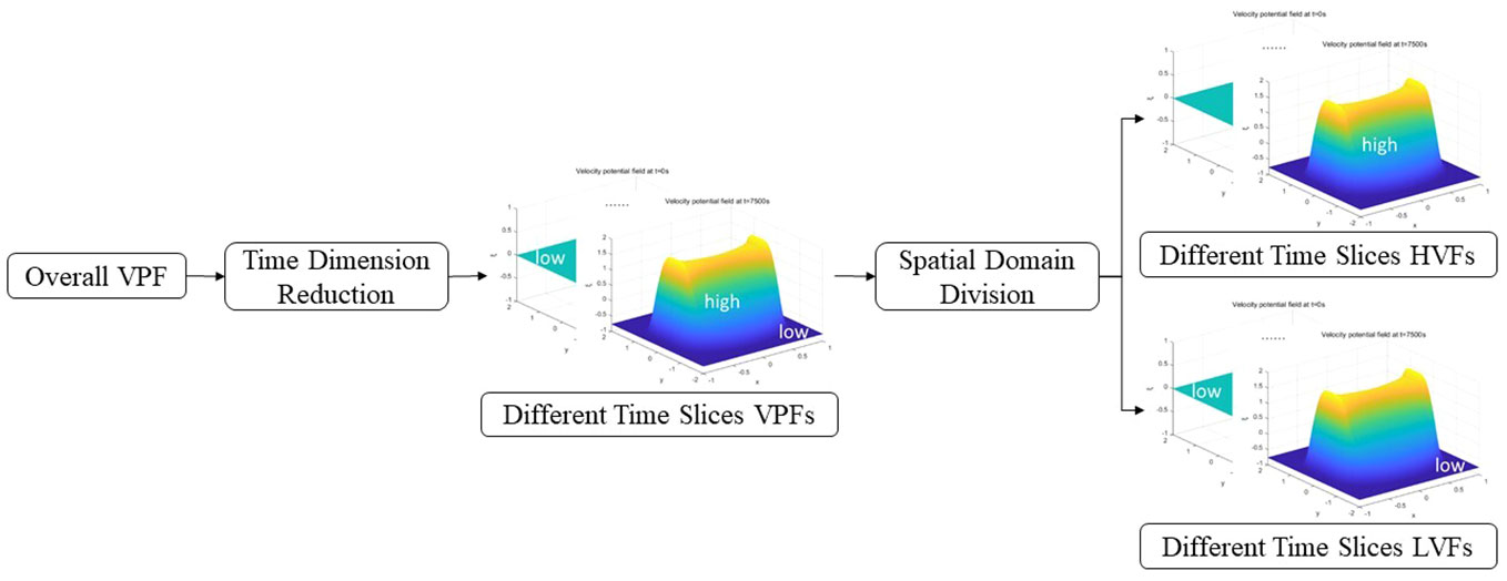
Figure 2 Temporal-spatial division module of overall velocity potential field.

Figure 3

Figure 3 Data rational selection module of multiple time slices.

In Figures 2–4, VPF is shorthand for velocity potential field, HVFs is shorthand for the high-velocity fields and HVF is the singular form of HVFs, LVFs is shorthand for the low-velocity fields and LVF is the singular form of LVFs.

In Figure 2, firstly, the whole velocity potential field with three-dimensional temporal-spatial data is temporal dimension reduced, and the velocity potential fields of different time slices are obtained. Then, the velocity potential field of different time slices is spatially divided, and the high-velocity field of different time slices (the raised part in middle marked by high) and the low-velocity field of different time slices (the smooth part in around marked by low) are obtained.

In Figure 3, firstly, the high-velocity field (low-velocity field) data of different time slices are divided into the data of the time slice to be solved and the data of the previous time slices. Then, the data of these two parts are selected reasonably, the data of the time slice to be solved are focused selected, and the data of the previous time slices are less selected, to obtain the reasonably selected data of the high-velocity field (low-velocity field).

In Figure 4, firstly, the reasonably selected data of the high-velocity field and the reasonably selected data of the low-velocity field are respectively input into parallel physics-informed neural networks (shown in Figure 5) of different servers for subdomain parallel calculation and the solved high-velocity field and the solved low-velocity field are obtained. Then, the subdomains solved by these two parts are combined in space to get the solved velocity potential field.

Figure 4

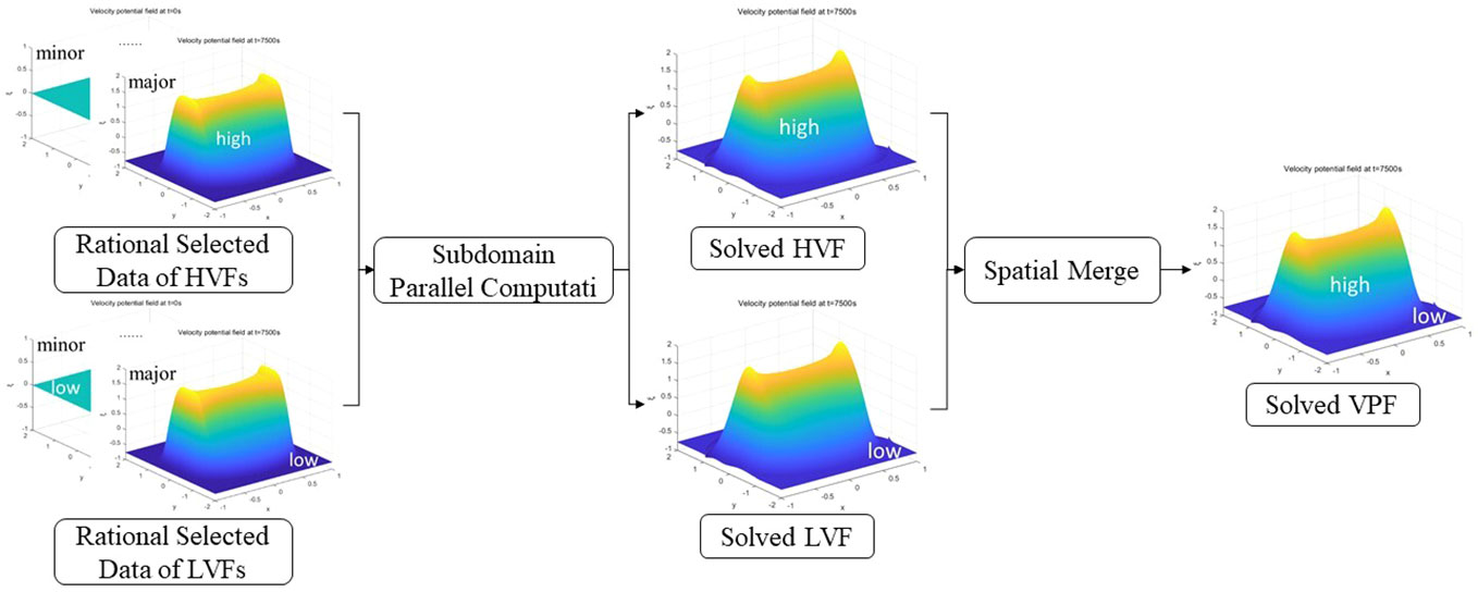
Figure 4 Parallel computation module of high-velocity fields and low-velocity fields.

Figure 5

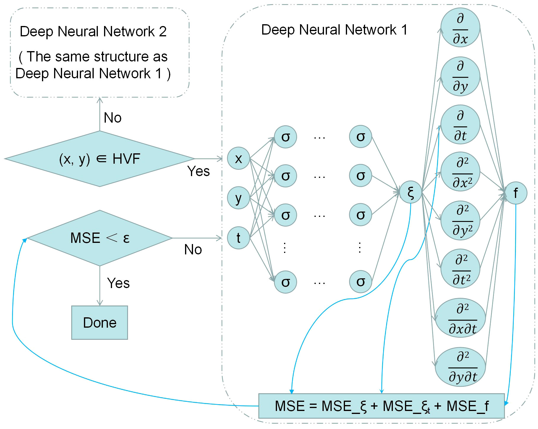
Figure 5 Network structure of DF-ParPINN.

3.2 Temporal-spatial division module of overall velocity potential field

3.2.1 mBL equation normalization

mBL equation has different velocity potential fields under different equation coefficients, initial conditions, and boundary conditions. The more coefficients of the equation, the more complex the initial and boundary conditions, and the more irregular the velocity potential field shape of mBL equation. The velocity potential field of mBL equation can be spatially domain divided according to regular shapes, and reduce complex high-dimensional nonconvexity. Therefore, in order to obtain the regular velocity potential field shape, we set the equation coefficients, initial conditions, and boundary conditions of mBL equation, and mBL equation after setting is shown in follows:

$\begin{array}{ll}{\xi }_{tt}-c^2\text{Δ}\xi -a\text{Δ}{\xi }_{tt}+\gamma [{(|\nabla \xi {\mid }^2)}_t+{\xi }_t\text{Δ}\xi ]=0& (13)\end{array}$

By setting the coefficient b in Equation 1 to 0, we get Equation 13. After the above settings, the velocity potential field of mBL equation can take on a regular shape.

3.2.2 Time dimension reduction

For mBL equation, the velocity potential fields of different time slices may have different shapes. Therefore, before spatial domain division of the velocity potential field, time dimension reduction is needed, that is, the overall velocity potential field is divided into velocity potential fields of different time slices based on the time axis. After the time dimension reduction, the original three-dimensional space-time mBL equation becomes many groups of the two-dimensional space mBL equation, and the complex high-dimensional non-convex characteristics of the mBL equation are degraded. In this way, DF-ParPINN does not have to process the three-dimensional data selected under all time slices at once, but only to process the three-dimensional data selected under the required time slices.

mBL equation of x ∈ [−1,1], y ∈ [−2,2] and t ∈ [0,7500] is taken as an example for time dimension reduction. Among them, x contains 512 points, y contains 1024 points, and t contains 51 time slices. After time dimensionality reduction, the overall velocity potential field, which originally contained 512*1024*51 = 26738688 solutions, was divided into 51 velocity potential fields corresponding to 51 time slices, each containing 512*1024 = 524288 solutions. The velocity potential fields at partial time slice solved by the pseudo-spectral method are shown in Figure 6:

Figure 6

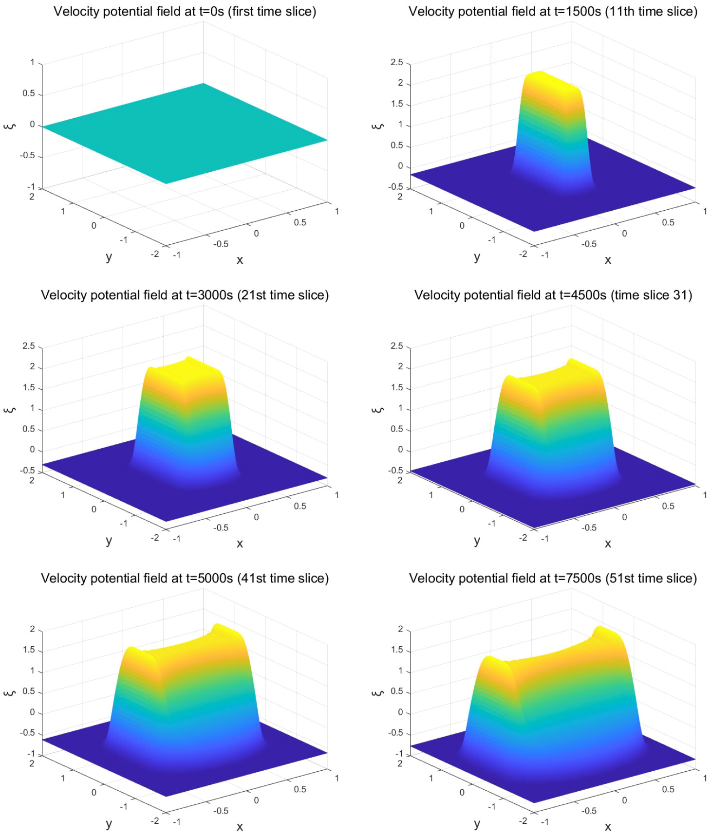
Figure 6 Velocity potential field at partial time slice solved by pseudo-spectral method.

3.2.3 Spatial domain division

As can be seen from Figure 6, for mBL equation, except that the initial field when t = 0 is “a flat land”, the velocity potential field of other time slices has a regular shape: high in the middle and low around the sides. Therefore, the velocity potential fields of different time slices can be spatially domain divided according to the shape of this rule. 51 sets of the high-velocity fields and the low-velocity fields can be obtained from 51 time slices. After the Spatial Domain Division, the original multiple velocity potential fields become multiple high-velocity and low-velocity fields, and the non-convex characteristics of mBL equation in space are further degraded. In this way, DF-ParPINN can process high-velocity fields and low-velocity fields separately, to better learn the characteristics of high-velocity fields and low-velocity fields.

For the velocity potential field per time slice (except for the initial field), the velocity potential values of some space points have a large variation range, and these space points are all distributed in the middle of the velocity potential field; the velocity potential values of other space points are almost unchanged, and these points are all distributed around the velocity potential field. The velocity potential field at this time can be divided into high-velocity potential field (referred to as “high-velocity field”) and low-velocity potential field (referred to as “low-velocity field”) based on the velocity threshold. The velocity threshold has the following characteristics: it is smaller than the value of all points in the high-velocity field and larger than the value of all points in the low-velocity field. Therefore, the high-velocity field is a part of the velocity potential field where the velocity potential of all points is greater than the velocity threshold, while the low-velocity field is another part of the velocity potential field where the velocity potential of all points is less than the velocity threshold. Because the velocity potential value of no space point is equal to the velocity threshold value, there are no boundary points and boundary domain when the velocity potential field is divided based on the velocity threshold value, and there is no sub neural network aiming at the boundary domain.

The velocity potential field at t = 7500s (51st time slice) of mBL equation is taken as an example to divide the spatial domain. For the velocity potential field at this time, the velocity threshold is -0.7616 when taking the minimum value of the velocity potential value of all space points by MATLAB (MATLAB takes four decimal places by default). Using -0.7616 as the velocity threshold, the velocity potential field at this time is spatially domain divided. The obtained high-velocity field, as shown in the middle trapezoid (yellow, green, and light blue) in Figure 6, contains 400762 space points. The obtained low-velocity field, as shown in the surrounding plane (dark blue) of Figure 6, contains 123526 space points.

3.3 Data rational selection module of multiple time slices

For the overall velocity potential field of mBL equation, it is difficult to obtain a high-accuracy solution by directly selecting a part of data from all time slices into PINN and outputting the solved velocity potential value of all time slices. This is because without dividing the overall velocity potential field, it is impossible to reduce its high-dimensional non-convex property, and the interaction of physical information in different time slices increases the complexity and difficulty of training. Therefore, in addition to the division of overall velocity potential field, the physical information of different time slices should be reasonably allocated. By selecting the data of different time slices reasonably, the physical information of different time slices can be allocated reasonably.

Objectively, the velocity potential value of mBL equation in a certain time slice depends only on the physical information of the current time slice and all previous time slices, and mainly depends on the physical information of the current time slice. Therefore, for the velocity potential field of a certain time slice, the physical information of all previous time slices should be related and the physical information of the current time slice should be focused during training. In other words, for the velocity potential field of a certain time slice, the data entered into the network for training should contain the data of the current time slice and all previous time slices, mainly including the data of the current time slice.

mBL equation of x ∈ [−1,1], y ∈ [−2, 2], and t ∈ [0,7500] is taken as an example to carry out reasonabledata selection. After the velocity potential field division module, the initial and boundary points of mBL equation are located in the initial field, and the velocity potential value of all space points in the initial field is zero. Moreover, the overall velocity potential field of mBL equation is divided into 51 groups (corresponding to 51 time slices) of high-velocity field and low-velocity field. When the high-velocity field and the low-velocity field of a certain time slice are required to be solved, the data entered into the network for training consists of two parts, as shown below:

$\begin{array}{ll}data=dat{a}_{i+}+dat{a}_{i-}& (14)\end{array}$

In Equation 14, data indicates all the selected data, data_i+ indicates the data selected from the time slice to be solved, and data_i− indicates the data selected from all previous time slices. The data contains space points and corresponding true velocity potential values, the amount of data in data_i+ is greater that in data_i−, and data_i− contains the data of the initial field.

3.4 Parallel computation module of high-velocity fields and low-velocity fields

The mBL equation of x ∈ [−1, 1], y ∈ [−2, 2] and t ∈ [0, 7500] is taken as an example of parallel computation in a subdomain. After the temporal-spatial division module of overall velocity potential field and the data rational selection module of multiple time slices, the overall velocity potential field of mBL equation is divided into 51 groups (corresponding to 51 time slices) of high-velocity field and low-velocity field. Moreover, when the high-velocity or the low-velocity field of a time slice is required to be solved, the data entered into the network contains not only the data of the time slice to be solved but also the data of all previous time slices. Compared with using a single server to serial compute the overall velocity potential field, using multiple servers to compute the high-velocity and the low-velocity fields of different time slices in parallel can accelerate the calculation speed. Therefore, when the velocity potential field of a certain time slice is required to be solved, different servers can be used to compute the high-velocity or the low-velocity field in parallel, and then combine the high-velocity field and the low-velocity field into one velocity potential field according to the spatial coordinates, as shown below:

$\begin{array}{ll}\xi ={\xi }_{high}\cup {\xi }_{low}& (15)\end{array}$

$\begin{array}{ll}{\xi }_{high}=[{\theta }_{high}(x,y,t)\mid (x,y)\in HVFs]& (16)\end{array}$

$\begin{array}{ll}{\xi }_{low}=[{\theta }_{low}(x,y,t)\mid (x,y)\in LVFs]& (17)\end{array}$

In Equations 15–17, ξ is the solved velocity potential value of the current velocity potential field, ξ_high is the solved velocity potential value of the current high-velocity field, and ξ_low is the solved velocity potential value of the current low-velocity field. θ_high is the neural network used by the current high-velocity field, and HV Fs is the current high-velocity field and all previous high-velocity fields. θ_low is the neural network used by the current low-velocity field, LV Fs is the current low-velocity field and all previous low-velocity fields, including the initial field, and the initial and boundary points are located in the initial field. ξ is obtained by the union of ξ_high and ξ_low. θ_high and θ_low have the same network structure is shown in Figure 5:

In the network structure of DF-ParPINN, the input is the space coordinates x, y and time coordinates t, and the output is the velocity potential value ξ and the function value f. The network first determines whether x and y belong to the high-velocity field, if yes, they are trained by deep neural network 1 in server 1, if not, they are trained by deep neural network 2 in server 2. The structure of the two deep neural networks is exactly the same, except that the inputs and outputs are different. x, y, t become ξ after deep neural network, ξ becomes multiple first and second partial derivatives after automatic derivation, and multiple partial derivatives become f when substituted into Equation 13. DF-ParPINN uses multiple deep neural networks in parallel to train the model and defines the loss function as:

$\begin{array}{ll}MSE=MS{E}_{\xi }+MS{E}_{{\xi }_t}+MS{E}_f& (18)\end{array}$

Where, MSE is the overall loss function, which is formed by adding MSE_ξ, MSE_ξt, and MSE_f.

$\begin{array}{ll}MS{E}_{\xi }=\frac{1}{N}\sum _N^{i=1}\mid \xi (x^i,y^i,t^i)-{\xi }^i\mid & (19)\end{array}$

Where MSE_ξ is the velocity potential loss function, ξ(x,y,t) is the velocity potential value solved by DF-ParPINN, ξ is the velocity potential value solved by the pseudospectral method, and N is the number of input space points in different time slices (including initial and boundary points). ξ in θ_high is ξ_high, and ξ in θ_low is ξ_low.

$\begin{array}{ll}MS{E}_{{\xi }_t}=\frac{1}{N}\sum _N^{i=1}\mid {\xi }_t(x^i,y^i,t^i)-{\xi }_t^i\mid & (20)\end{array}$

Where, MSE_ξt is the first-order partial time derivative loss function, ξ_t(x,y,t) is the first partial derivative of ξ to t solved by DF-ParPINN, ξ_t is the first partial derivative of ξ to t solved by the pseudospectral method, and N is the number of input space points in different time slices (including initial and boundary points). ξ_t in θ_high is ξ_thigh, and ξ_t in θ_low is ξ_tlow.

$\begin{array}{ll}MS{E}_f=\frac{1}{N}\sum _N^{i=1}\mid f(x^i,y^i,t^i)-f^i\mid & (21)\end{array}$

Where, MSE_f is the physical information loss function, f(x,y,t) is the size of mBL equation solved by DF-ParPINN, f is the size of mBL equation solved by the pseudo-spectral method, and N is the number of input space points in different time slices (include initial and boundary points). f in θ_high is f_high, and f in θ_low is f_low.

Moreover, θ_low is also responsible for processing the data of the initial field, and the initial and boundary points are located in the initial field, and the loss function of the initial and boundary points also follows Equations 18-21.

If DF-ParPINN can solve mBL equation well, then the velocity potential value of MSE_ξ with respect to every point tends to zero, the first partial derivative of MSE_ξt with respect to every point tends to zero, and the physical equation value of MSE_f with respect to every point tends to zero. In other words, when MSE approaches zero, it can be considered that the solved value of each point on the training data set approaches the true value. In this way, solving mBL equation is transformed into an optimization loss function using the backpropagation mechanism of the neural network and two optimizers, L-BFGS and Adam.

4 Results

4.1 Data set

We use mBL equation with the regular shape shown in Equation 13 to conduct numerical experiments, and the data set was obtained and provided by Chunxin Yuan et al. through the pseudo-spectral method. The detailed information of mBL equation dataset is shown in Table 1:

Table 1

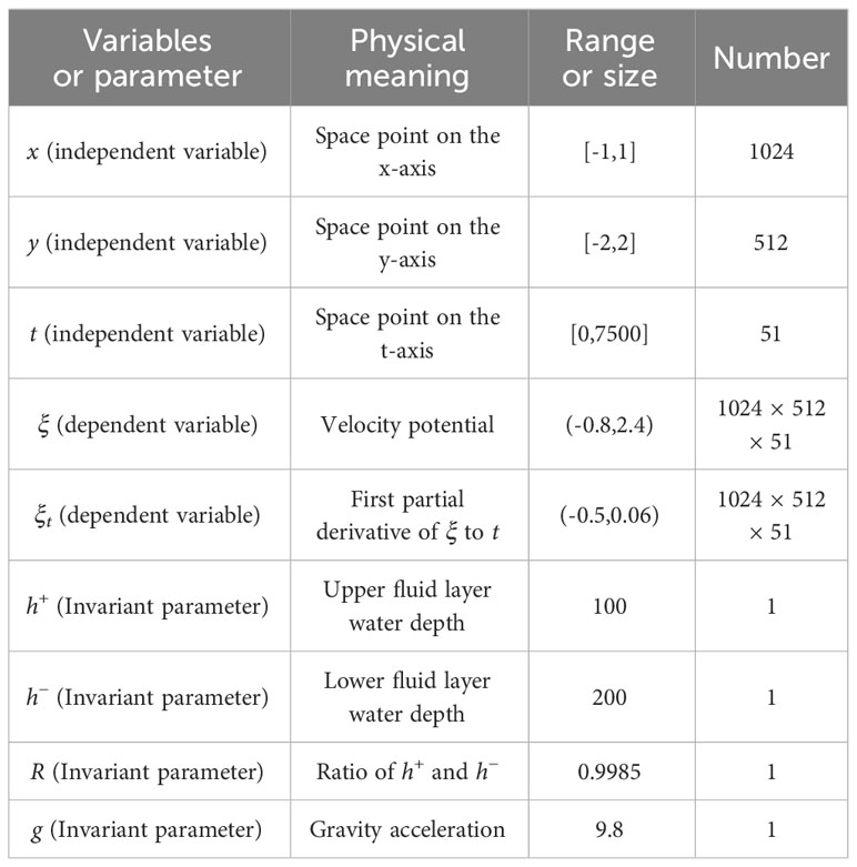
Table 1 Detailed information of mBL equation data set.

4.2 Initial conditions and boundary conditions

For mBL equation shown in Equation 13, there are many sets of initial conditions and boundary conditions, but not every set of conditions results in a mBL equation with the regular shape. The initial conditions and boundary conditions of mBL equation with the regular shape are shown in Table 2:

Table 2

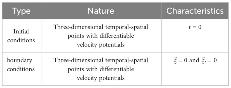
Table 2 Initial conditions and boundary conditions of mBL equation with the regular shape.

4.3 Comparative study

4.3.1 Experimental setup

In order to verify that DF-ParPINN can solve mBL equation with high accuracy, we use three physical information neural network methods PINN, PIRNN, and cPINN, and a neural computing subclass method DeepONet, as the contrast baseline. The differences between the five algorithms are shown in Table 3:

Table 3

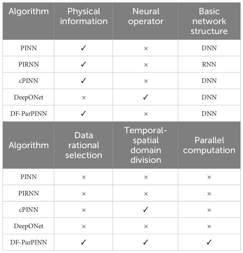
Table 3 Differences between the five algorithms (contrast experiments).

The input and output of the five algorithms are shown in Table 4:

Table 4

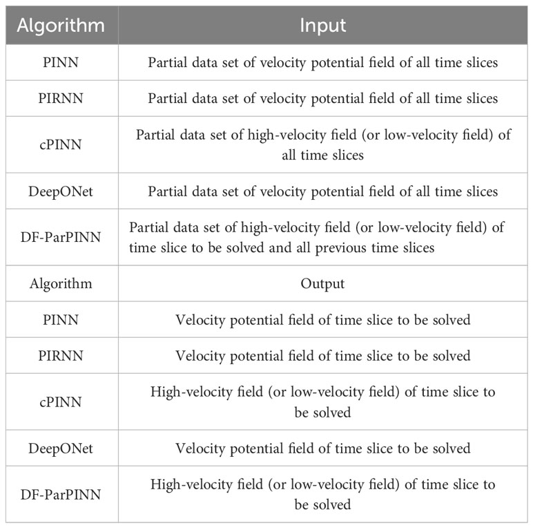
Table 4 Input and output of the five algorithms (contrast experiments).

The detailed settings of the five algorithms are shown in Table 5:

Table 5

Table 5 Detailed settings of the five algorithms (contrast experiments).

Both the training set and the test set of the five algorithms belong to the same data set, both follow the principle of random selection, and the data contained in both are not repeated.

PINN or PIRNN does not perform temporal-spatial domain division of mBL equation. PINN or PIRNN selected directly 100000 datasets from 1024 × 512 × 51 datasets (containing the overall velocity potential field of all time slices) as the training set, and 10000 datasets from 1024 × 512 datasets (containing only the velocity potential field of the time slice to be solved) as the test set.

cPINN only performs temporal-spatial domain division (division only in the spatial domain), and divides the velocity potential field of all time slices into the overall high-velocity field and the overall low-velocity field. For the overall high-velocity field, cPINN selected 100000 datasets from 400762*51 datasets (containing the high-velocity field and the partial low-velocity field of all time slices) as the training set, and selected 10000 datasets from 400762 datasets (containing the high-velocity field and the partial low-velocity field of the time slices to be solved) as the test set. For the overall low-velocity field, cPINN selected 10000 datasets from 123526*51 datasets (containing another part of the low-velocity field of all time slices) as the training set, and selected 10000 datasets from 123526 datasets (containing another part of the low-velocity field of the time slice to be solved) as the test set.

DeepONet does not perform temporal-spatial domain division of mBL equation. The training set and test set selection of DeepONet are the same as that of PINN.

DF-ParPINN performs temporal-spatial domain division (division in both spatial and temporal domains) for mBL equation, and divides the velocity potential field of each time slice into two parts: the high-velocity field and the low-velocity field. For the high-velocity field (the low-velocity field) of the time slice to be solved, DF-ParPINN first selected 95000 datasets from the high-velocity field (the low-velocity field) of the time slice to be solved, then selected 5000 datasets from high-velocity fields (the low-velocity field) of all previous time slices, a total of 100000 datasets were selected as training sets, and selected 10000 datasets from the high-velocity field (the low-velocity field) of the time slice to be solved. Unlike cPINN, which only uses a single server to train and test the overall high-velocity field and the overall low-velocity field, DF-ParPINN uses multiple servers to train and test the high-velocity field and the low-velocity field separately in parallel, to improve the training and testing speed under the spatial-temporal division strategy.

For mBL equation, cPINN divides the velocity potential field of all time slices based on the velocity threshold of the last time slice, and DF-ParPINN divides the velocity potential field of each time slice based on the velocity threshold of each time slice. Because the velocity potential value of no space point is equal to the velocity threshold, there is no boundary point and boundary domain when the velocity potential field is divided based on the velocity threshold, and there is no sub-neural network for the boundary domain.

In solving equations, PINN uses relative error to measure the accuracy of the solution. Therefore, in solving mBL equation, the five algorithms continue to use relative error to measure the accuracy of the velocity potential field solved. In this paper, the relative error is the matrix of two norms between the algorithm prediction solution and the pseudo-spectral method numerical solution. The smaller the relative error is, the higher the accuracy of the prediction solution is, and the better the performance of the algorithm is. For the algorithms that use temporal-spatial domain division, the relative error of the velocity potential field of the time slice to be solved is shown as follows:

$\begin{array}{ll}error=(h\times erro{r}_h)+(l\times erro{r}_l)& (22)\end{array}$

$\begin{array}{ll}h=\frac{coun{t}_h}{count}, l=\frac{coun{t}_l}{count}& \text{(23, 24)}\end{array}$

In Equations 23, 24, error is the relative error of the velocity potential field of the time slice to be solved, error_h is the relative error of the high-velocity field of the time slice to be solved, error_l is the relative error of the low-velocity field of the time slice to be solved, count_h is the number of space points of the overall high-velocity field (cPINN) or the number of space points of the high-velocity field of the time slice to be solved (DF-ParPINN). count_l is the number of space points in the overall low-velocity field (cPINN) or the number of space points in the low-velocity field of the time slice to be solved (DF-ParPINN), and count is the number of space points in the overall velocity potential field (cPINN) or the number of space points in the velocity potential field of the time slice to be solved (DF-ParPINN).

4.3.2 Experimental results

After the above settings, five algorithms are trained separately on the same mBL equation data set, and partial time slice data is selected for testing. The relative errors of the five algorithms are shown in Table 6:

Table 6

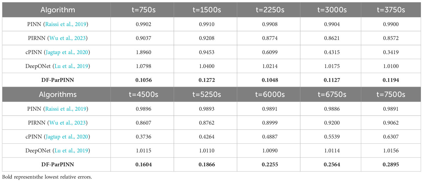
Table 6 Relative errors of the five algorithms (contrast experiments).

The solution time of the five algorithms is shown in Table 7:

Table 7

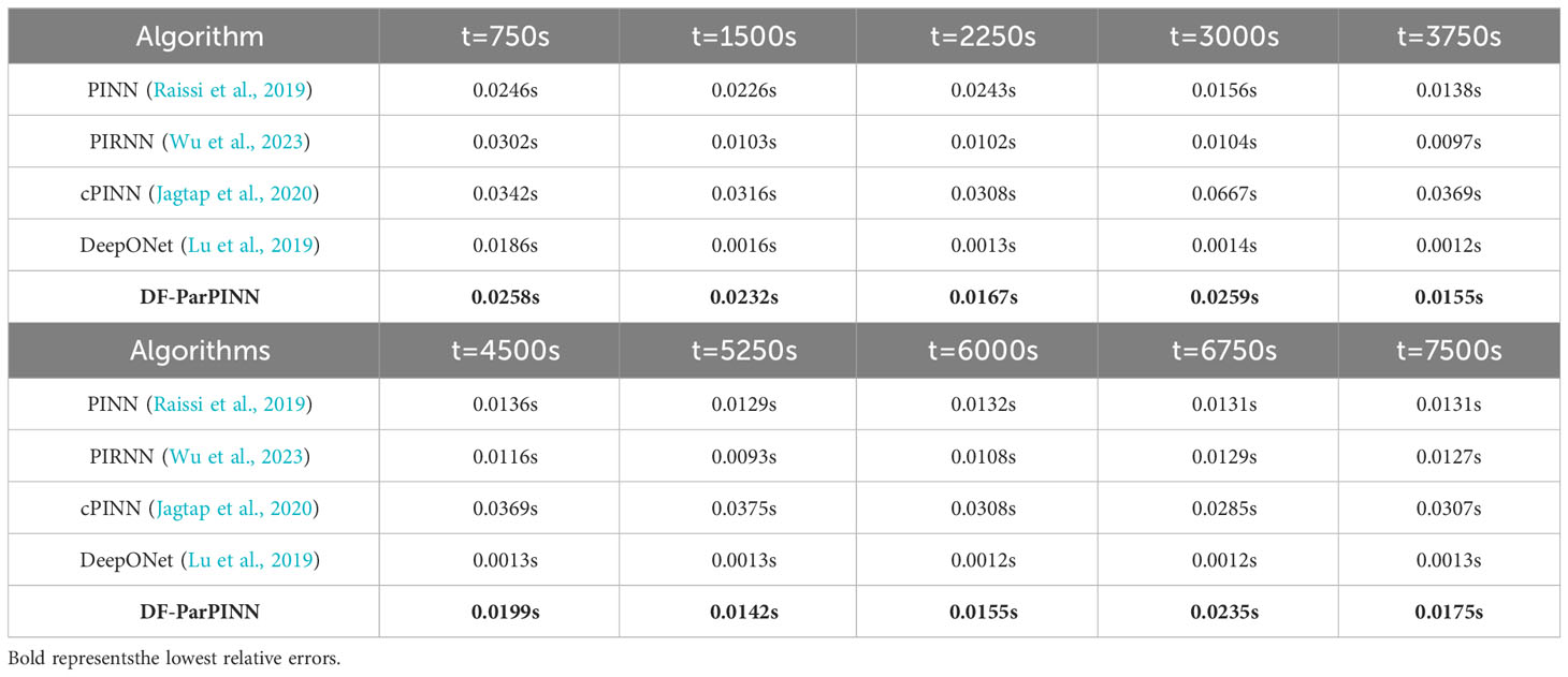
Table 7 Solution time of the five algorithms (contrast experiments).

Where, t=750s is the 6th time slice, t=1500s is the 11st time slice, t=2250s is the 16th time slice, t=3000s is the 21st time slice, t=3750s is the 26th time slice, t=4500s is the 31st time slice, t=5250s is the 36th time slice, t=6000s is the 41st time slice, t=6750s is the 46th time slice, t=7500s is the 51st time slice.

It can be clearly seen from Table 6 that compared with PINN, PIRNN, cPINN, and DeepONet, DFParPINN has absolute accuracy advantages in solving mBL equation, which proves that DF-ParPINN is the most effective. It also can be clearly seen from Table 7 that the average solution time of the five algorithms is no more than 0.5s, much faster than 9.4 minutes of the pseudo-spectral method, which proves that DF-ParPINN is very efficient.

4.4 Ablation study

4.4.1 Experimental setup

In addition to comparison experiments, we also conducted ablation experiments to further verify the effectiveness of DF-ParPINN. The ablation experiments adopt module ablation and include three modules. Temporal-spatial division module of overall velocity potential field is the first module, data rational selection module of multiple time slices is the second module, parallel computation module of high-velocity fields and low-velocity fields is the third module. The first module is the premise for the second and the third module, without the first module there can be no the second and the third module. The second module can be divided into the first submodule data rational selection and the second submodule data focus. The second module can be divided into the first submodule data focus and the second submodule data rational selection. The first submodule is the premise of the second submodule data, without the first submodule there is no second submodule. Therefore, five ablation algorithms can be set up. The differences between the five algorithms are shown in Table 8:

Table 8

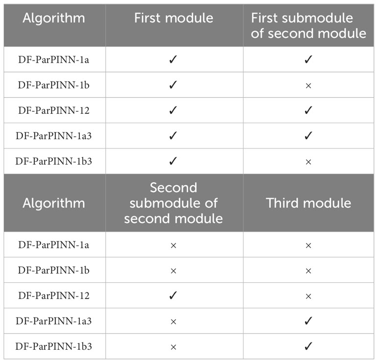
Table 8 Differences between the five algorithms (ablation experiments).

The input and output of the five algorithms are shown in Table 9:

Table 9

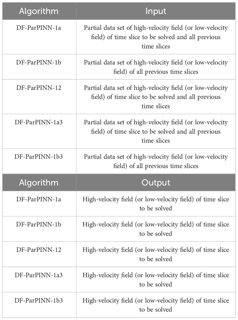
Table 9 Input and output of the five algorithms (ablation experiments).

The detailed settings of five algorithms are shown in Table 10:

Table 10

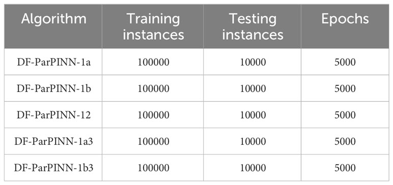
Table 10 Detailed settings of five algorithms (ablation experiments).

Both the training set and the test set of the five algorithms belong to the same data set, both follow the principle of random selection, and the data contained in both are not repeated.

DF-ParPINN-1a or DF-ParPINN-1a3 do not select data from datasets of the time slice to be solved and datasets of all previous time slices according to the 95000:5000 allocation rule, but more focus on selecting data from datasets of the time slices to be solved. For the high-velocity field (the low-velocity field) of the time slice to be solved, the algorithm first selected 50000 datasets from the high-velocity field (the low-velocity field) of the time slice to be solved, then selected 50000 datasets from high-velocity fields (low-velocity fields) of all previous time slices, a total of 100000 datasets were selected as training sets, and selected 10000 datasets from the high-velocity field (the low-velocity field) of the time slice to be solved as test sets. DF-ParPINN-1a3 also uses different servers to solve high-velocity and low-velocity fields.

DF-ParPINN-1b or DF-ParPINN-1b3 do not select data from datasets of the time slice to be solved and datasets of all previous time slices according to the 95000:5000 allocation rule, and do not focus on selecting data from datasets of the time slices to be solved. For the high-velocity field (the low-velocity field) of the time slice to be solved, the algorithm selected directly 100000 datasets from all high-velocity fields (all low-velocity fields) of all time slices as training sets, and selected 10000 datasets from the high-velocity field (the low-velocity field) of the time slice to be solved as test sets.DF-ParPINN-1b3 also uses different servers to solve high-velocity and low-velocity fields.

DF-ParPINN-12 selects data from datasets of the time slice to be solved and datasets of all previous time slices according to the 95000:5000 allocation rule. For the high-velocity field (the low-velocity field) of the time slice to be solved, the algorithm first selected 5000 datasets from the high-velocity field (the low-velocity field) of the time slice to be solved, then selected 95000 datasets from high-velocity fields (low-velocity fields) of all previous time slices, a total of 100000 datasets were selected as training sets, and selected 10000 datasets from the high-velocity field (the low-velocity field) of the time slice to be solved as test sets. DF-ParPINN-1a3 does not use different servers to solve high-velocity and low-velocity fields.

In solving mBL equation, we still use relative error to measure the accuracy of the velocity potential field solved by the five algorithms. For DF-ParPINN, the relative error of the velocity potential field of the time slice to be solved is shown in Equation 22).

4.4.2 Experimental results

After the above settings, five algorithms are trained separately on the same mBL equation data set, and partial time slice data is selected for testing. With the addition of DF-ParPINN, the relative errors of the six algorithms are shown in Table 11:

Table 11

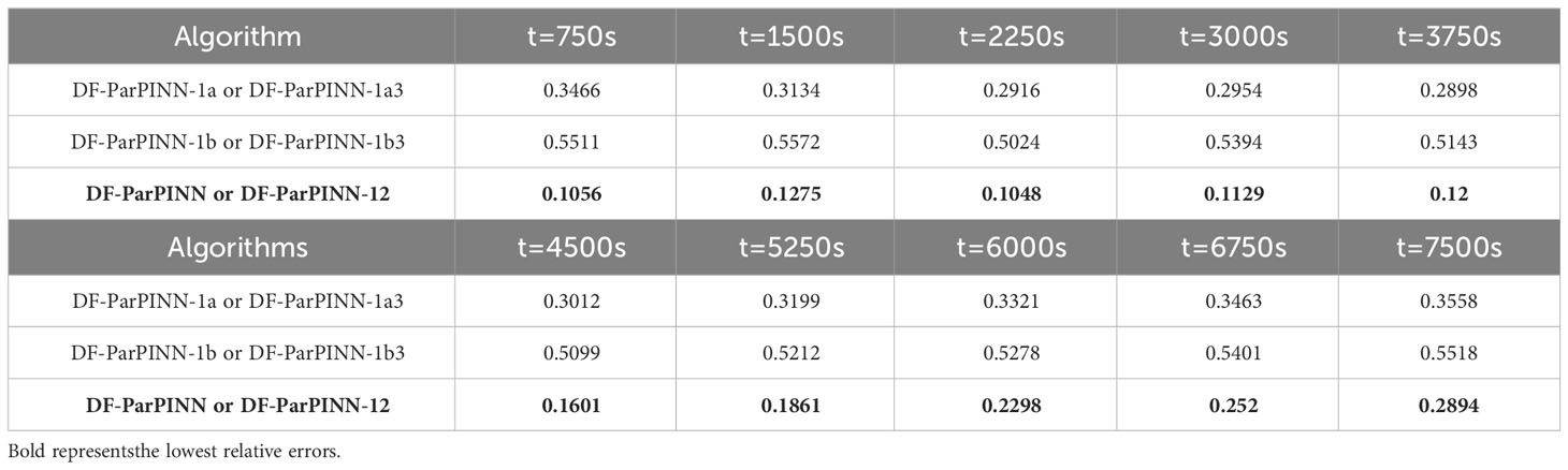
Table 11 Relative errors of the six algorithms (ablation experiments).

The solution time of the six algorithms is shown in Table 12:

Table 12

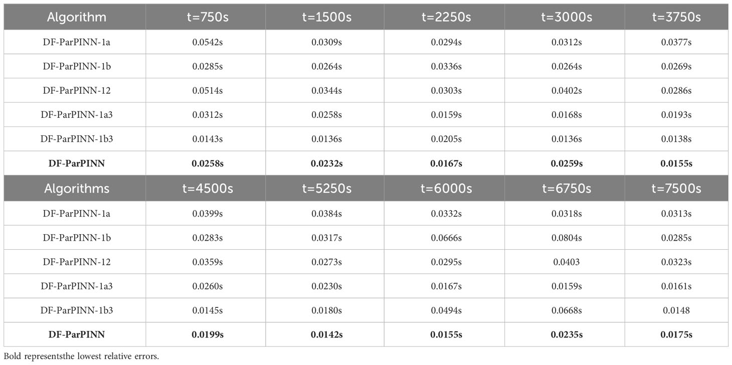
Table 12 Solution time of the six algorithms (ablation experiments).

It can be clearly seen from Table 11 that compared with DF-ParPINN-1a, DF-ParPINN-1b, DF-ParPINN1a3, and DF-ParPINN-1b3, DF-ParPINN and DF-ParPINN-12 have same absolute accuracy advantages in solving mBL equation, which proves that DF-ParPINN is the most effective. It also can be clearly seen from Table 12 that the average solution time of DF-ParPINN, DF-ParPINN-1a, DF-ParPINN-1b, DF-ParPINN-12, DF-ParPINN-1a3 and DF-ParPINN-1b3 is 0.0198s, 0.0358s, 0.0207s, 0.0350s and 0.0239s respectively, and the average solution time of DF-ParPINN is the shortest, which proves that DF-ParPINN is the most efficient.

4.5 Depth study

4.5.1 Experimental setup

Unlike PINN, PIRNN, cPINN, and DeepONet, which use only one optimizer for training, DF-ParPINN can use both LBFGS and Adam optimizers for deep training. First use LBFGS efficient training, when the epochs reach 10000, the loss no longer decreases. Then use Adam to continue training, until the loss is almost no longer decreasing.

4.5.2 Experimental results

Taking the velocity potential field at t=7500s (51st time slice) of mBL equation as an example, the depth training of DF-ParPINN was conducted. The training set is consistent with the description in 4.2.1, while the test set changes to all 400762 datasets of high-velocity field at t=7500s and all 123526 datasets of low-velocity field at t=7500s. The relative errors in different training stages are shown in Table 13:

Table 13

Table 13 Relative errors in different training stages (depth experiments).

The solution time in different training stages is shown in Table 14:

Table 14

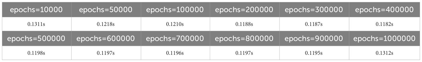
Table 14 Solution time in different training stages (depth experiments).

Finally, after deep training 1000000 epochs, the velocity potential field t=7500s solved by DF-ParPINN is shown in the left part of Figure 7, and the velocity potential field t=7500s solved by the pseudo-spectral method is shown in the right part of Figure 7:

Figure 7

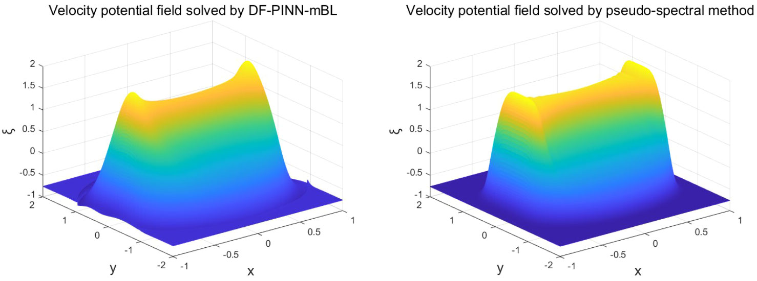
Figure 7 Velocity potential field at t=7500s solved by two algorithms.

Comparing the left and right parts of Figure 7, the velocity potential field solved by DF-ParPINN after deep training 1000000 epochs almost fits the velocity potential field solved by the pseudo-spectral method, which further proves DF-ParPINN is very effective. It also can be clearly seen from Table 14 that the average solution time of DF-ParPINN after deep training is still no more than 0.5s, much faster than 9.4 minutes of the pseudo-spectral method, which proves that DF-ParPINN is very efficient.

5 Discussion

5.1 Compared with advanced deep learning PDE solvers

mBL equation is a high-dimensional non-convex function with three-dimensional spatiotemporal variables, and high-dimensional non-convex optimization problems are NP-hard problems that are difficult to solve accurately. Therefore, PINN is easy to fall into the local optimal solution when solving mBL equations, so it is difficult to obtain the exact solution, so the overall accuracy of PINN is not ideal.

Compared with PINN, PIRNN uses RNN to replace the DNN in PINN. The circular structure of RNN allows information to be passed between different time steps, captures long-term dependencies, and exploits contextual information. These make RNN better model the timing relationship of velocity potential fields in different time slices, and then improve the solving accuracy, so the overall accuracy of PIRNN is higher than that of PINN.

Compared with PINN, cPINN uses the same spatial domain partitioning strategy for velocity potential fields in different time slices, and divides the overall velocity potential field into two parts: the overall high-velocity field and the overall low-velocity field, which have different spatial characteristics. Therefore, first solving the overall high-velocity field and the overall low-velocity field, then combining them can reduce the difficulty of solving, and then improve the solving accuracy, so the overall accuracy of cPINN is higher than that of PINN.

DeepONet does not use the corresponding physical information to assist in solving mBL equations, and the complex high-dimensional characteristics of mBL equations are very challenging for DeepONet neural operators. As a result, it is difficult for DeepONet to accurately capture all the details and features of mBL equation, so the overall accuracy of DeepONet is lower than other algorithms.

DF-ParPINN uses three modules: the temporal-spatial division module of the overall velocity potential field, the data rational selection module of multiple time slices, and the parallel computation module of high-velocity and low-velocity fields. These modules improve the PINN, to a certain extent, and solve the following three problems that exist when the PINN solves PDEs: difficult to solve complex PDEs with high-dimensional non-convex properties, difficult to transfer the physical information of boundary points and initial points, and difficult to train the automatic derivative network quickly at a low cost. Therefore, DF-ParPINN greatly improves the accuracy of solving the mBL equation, so the overall accuracy of DF-ParPINN is higher than that of other algorithms.

5.2 Compared with DF-ParPINN with different modules

DF-ParPINN-1a or DF-ParPINN-1a3 uses the temporal-spatial division module of overall velocity potential field, but uses only the data focus submodule of the data rational selection module of multiple time slices. Because the amount of data selected from the velocity potential field of the time slice to be solved is the same as the velocity potential fields of all previous time slices, the physical information of the velocity potential field of the time slice to be solved is not utilized to the maximum extent, so their accuracy is not ideal.

Compared with DF-ParPINN-1a, DF-ParPINN-1a3 also uses the parallel computation module of highvelocity fields and low-velocity fields, replacing the serial computation of a single server used by the DF-ParPINN-1a with parallel computation of multiple servers, which greatly reduces the training time and significantly reduces the solution time.

DF-ParPINN-1b or DF-ParPINN-1b3 uses the temporal-spatial division module of overall velocity potential field, but does not use the data rational selection module of multiple time slices. Due to the lack of focused and reasonable distribution of training data, the physical information of velocity potential fields of all previous time slices is overused, so their accuracy is not ideal.

Compared with DF-ParPINN-1b, DF-ParPINN-1b3 also uses the parallel computation module of highvelocity fields and low-velocity fields, replacing the serial computation of a single server used by the DF-ParPINN-1b with parallel computation of multiple servers, which greatly reduces the training time and significantly reduces the solution time.

Compared with DF-ParPINN, DF-ParPINN-12 just doesn’t use the parallel computation module of high-velocity fields and low-velocity fields, instead using a single server for serial computation. Therefore, the solution accuracy of both is the same, but the training time of DF-ParPINN-12 is much larger than that of DF-ParPINN, and the solution time is significantly larger than that of DF-ParPINN.

DF-ParPINN uses all three modules, and to a certain extent solves the three problems that exist when PINN solves PDE, so the accuracy of DF-ParPINN is the highest.

5.3 Compared with DF-ParPINN after deep training

DF-ParPINN trained only 5000 epochs using the LBFGS optimizer, and the training loss only converges to a local minimum, so the accuracy of DF-ParPINN is not very low.

DF-ParPINN after deep training uses LBFGS and Adam two optimizers to train more than 10000 epochs, and when epochs reach 1000000 the training loss almost converges to the global minimum, so the accuracy of DF-ParPINN after deep training is close to ideal.

5.4 Limitations of DF-ParPINN

First, DF-ParPINN needs to perform the temporal-spatial division of the PDE. If there are too many time slices of the PDE or the space field shape of each time slice is irregular, it is difficult to perform the temporal-spatial division.

Secondly, DF-ParPINN needs to perform the data rational selection of different time slices, which depends on the temporal-spatial division of the PDE. If the time dimension reduction is unsuccessful, it is difficult to perform the data rational selection.

Finally, DF-ParPINN needs to perform the parallel computation of different types of fields, which also depends on the temporal-spatial division of the PDE, and if the spatial division is not successful, it is difficult to perform the parallel computation.

Therefore, some very complex high-dimensional PDEs in real-world applications have no regular shape, the current DF-ParPINN has difficulty solving them.

6 Conclusion

In order to solve mBL equation, a high-dimensional PDE with complex structures, quickly and accurately, and achieve a new breakthrough in solving complex PDE of the physical ocean field by using deep learning technology, we propose “DF-ParPINN: parallel PINN based on velocity potential field division and single time slice focus”. DF-ParPINN consists of three modules: temporal-spatial division module of overall velocity potential field, rational selection module of multiple time slices data, and parallel computation module of high-velocity fields and low-velocity fields, each of them respectively realizes the optimization of the high-dimensional non-convex equation, the deep transmission of effective physical information, the low cost and fast training of the network, to varying degrees. The core of DF-ParPINN is parallel physics-informed neural networks of different servers, they are used separately to solve the high-velocity field and low-velocity field. The experimental results show that the solution time of DF-ParPINN is no more than 0.5s, and its accuracy is much higher than that of PINN, PIRNN, cPINN, and DeepONet. Moreover, the relative error of DF-ParPINN after deep training 1000000 epochs can be reduced to less than 0.1. With the help of neural operators and other methods, continue to improve DF-ParPINN, so that it can solve more complex mBL equations more accurately and quickly, which will be our future research direction.

Data availability statement

The raw data supporting the conclusions of this article will be made available by the authors, without undue reservation.

Author contributions

JC: Conceptualization, Data curation, Formal analysis, Methodology, Software, Visualization, Writing – original draft, Writing – review & editing. CY: Conceptualization, Resources, Validation, Writing – review & editing. JX: Funding acquisition, Methodology, Resources, Validation, Writing – review & editing. PB: Data curation, Software, Writing – review & editing. ZW: Funding acquisition, Resources, Writing – review & editing.

Funding

The author(s) declare financial support was received for the research, authorship, and/or publication of this article. This research was supported in part by the Key Research and Development Projects of Shandong Province (2019JMRH0109).

Conflict of interest

The authors declare that the research was conducted in the absence of any commercial or financial relationships that could be construed as a potential conflict of interest.

Publisher’s note

All claims expressed in this article are solely those of the authors and do not necessarily represent those of their affiliated organizations, or those of the publisher, the editors and the reviewers. Any product that may be evaluated in this article, or claim that may be made by its manufacturer, is not guaranteed or endorsed by the publisher.

References

Abel G. P., Roca X., Peraire J., Sarrate J. (2013). Defining Quality Measures for Validation and Generation of High-Order Tetrahedral Meshes (Hoboken: John Wiley and Sons Ltd).

Google Scholar

Benney D. J., Luke J. C. (1964). On the interactions of permanent waves of finite amplitude. Stud. Appl. Mathematics. 43 (1-4), 309–313. doi: 10.1002/sapm1964431309

CrossRef Full Text | Google Scholar

Chen X. H., Liu J., Pang Y. F., Chen J., Gong C. Y. (2020). Developing a new mesh quality evaluation method based on convolutional neural network. Eng. Appl. Comput. Fluid Mechanics 14, 391–400. doi: 10.1080/19942060.2020.1720820

CrossRef Full Text | Google Scholar

Han J., Arnulf J., Weinan E. (2018). Solving high-dimensional partial differential equations using deep learning. Proc. Natl. Acad. Sci. 115 (34), 8505–8510. doi: 10.1073/pnas.1718942115

CrossRef Full Text | Google Scholar

Jagtap A. D., Kharazmi E., Karniadakis G. E. (2020). Conservative physics-informed neural networks on discrete domains for conservation laws: Applications to forward and inverse problems. Comput. Methods Appl. Mechanics Eng. 365, 113028. doi: 10.1016/j.cma.2020.113028

CrossRef Full Text | Google Scholar

Kadomtsev B. B., Petviashvili V. I. (1970). On the stability of solitarywaves inweakly dispersive media. (Russian Academy of Sciences, SPB)

Google Scholar

Katz A., Sankaran V. (2011). Mesh quality effects on the accuracy of cfd solutions on unstructured meshes. J. Comput. Phys. 230, 7670–7686. doi: 10.1016/j.jcp.2011.06.023

CrossRef Full Text | Google Scholar

Le C. (2022). Ai for science: Innovate the future together - 2022 zhongguancun forum series activities “science intelligence summit” held. Zhongguancun 2, 40–41.

Google Scholar

Li Y., Cheng C. S. (2022). Physics-informed neural networks: Recent advances and prospects. Comput. Sci. 49(4), 254–262. doi: 10.11896/jsjkx.210500158

CrossRef Full Text | Google Scholar

Lu J. F., Guan Z. (2004). Numerical Solving Methods of Partial Differential Equations. 2nd (Beijing: Tsinghua University Press).

Google Scholar

Lu L., Jin P., Karniadakis G. E. (2019). Deeponet: Learning nonlinear operators for identifying differential equations based on the universal approximation theorem of operators. ArXiv, ITH

Google Scholar

Lu Z. B., Qu J. H., Liu H., He C., Zhang B. J., Chen Q. L. (2021). Surrogate modeling for physical fields of heat transfer processes based on physics-informed neural network. CIESC J. 72 (3), 1496–1503. doi: 10.11949/0438-1157.20201879

CrossRef Full Text | Google Scholar

Molinet L., Saut J. C., Tzvetkov N. (2011). Global well-posedness for the kp-ii equation on the background of a non-localized solution. Commun. Math. Phys. 28, 653–676. doi: 10.1016/j.anihpc.2011.04.004

CrossRef Full Text | Google Scholar

Nabian M. A., Meidani H. (2019). A deep learning solution approach for highdimensional random differential equations - sciencedirect. Probabilistic Eng. Mechanics 57, 14–25. doi: 10.1016/j.probengmech.2019.05.001

CrossRef Full Text | Google Scholar

Ockendon J., Howison S., Lacey A., Movchan A. (2003). Applied Partial Differential Equations (New York: Oxford University Press).

Google Scholar

Raissi M., Karniadakis G. E. (2018). Hidden physics models: Machine learning of nonlinear partial differential equations. J. Comput. Phys. 357, 125–141. doi: 10.1016/j.jcp.2017.11.039

CrossRef Full Text | Google Scholar

Raissi M., Perdikaris P., Karniadakis G. E. (2017a). Numerical gaussian processes for time-dependent and non-linear partial differential equations. Siam J. Sci. Computing 40, A172–A198. doi: 10.1137/17M1120762

CrossRef Full Text | Google Scholar

Raissi M., Perdikaris P., Karniadakis G. E. (2017b). Physics informed deep learning (part I): Data-driven solutions of nonlinear partial differential equations. ArXiv, ITH.

Google Scholar

Raissi M., Perdikaris P., Karniadakis G. E. (2017c). Physics informed deep learning (part II): Data-driven discovery of nonlinear partial differential equations. ArXiv, ITH.

Google Scholar

Raissi M., Perdikaris P., Karniadakis G. E. (2019). Physics-informed neural networks: A deep learning framework for solving forward and inverse problems involving nonlinear partial differential equations. J. Comput. Phys. 378, 686–707. doi: 10.1016/j.jcp.2018.10.045

CrossRef Full Text | Google Scholar

Science (2016). Science publishes 125 cutting-edge questions in science. Field Vision 2, 54–55.

Google Scholar

Shao S., Lei Y. M., Lan H. Q. (2022). Traveltime calculation for complex models based on physicsinformed neural networks. Prog. Geophysics. 37 (5), 1840–1853. doi: 10.6038/pg2022FF0474

CrossRef Full Text | Google Scholar

Shi Z. C. (2001). The third scientific method – scientific calculation in the computer age. Encyclopedic Knowledge 3, 9–11.

Google Scholar

Wang N., Chang H., Zhang D. (2021). Deep-learning-based inverse modeling approaches: A subsurface flow example. John Wiley Sons Ltd. 126 (2), e2020JB020549. doi: 10.1029/2020JB020549

CrossRef Full Text | Google Scholar

Weinan E., Han J., Jentzen A. (2017). Deep learning-based numerical methods for high-dimensional parabolic partial differential equations and backward stochastic differential equations. 5(4), 349–380. doi: 10.1007/s40304-017-0117-6

CrossRef Full Text | Google Scholar

Wu G., Yion W. T. G., Dang K. L. N. Q., Wu Z. (2023). Physics-informed machine learning for mpc: Application to a batch crystallization process. Chem. Eng. Res. Design 192, 556–569. doi: 10.1016/j.cherd.2023.02.048

CrossRef Full Text | Google Scholar

Xu H. (2021). Dl-pde: Deep-learning based data-driven discovery of partial differential equations from discrete and noisy data. Commun. Comput. Phys. 29, 698–728. doi: 10.4208/cicp.OA-2020-0142

CrossRef Full Text | Google Scholar

Yuan C. X., Wang Z. (2022). On diffraction and oblique interactions of horizontally two-dimensional internal solitary waves. J. Fluid Mechanics. 936, A20. doi: 10.1017/jfm.2022.60

CrossRef Full Text | Google Scholar

Zheng S., Lin Y. Y., Feudal L., Jin F. (2022). Viscous regularization pinn algorithm for shallow water wave equations. Chin. J. Comput. Phys. 40 (3), 314–324. doi: 10.19596/j.cnki.1001-246x.8592

CrossRef Full Text | Google Scholar