 Jesse M. Vance
 Kim Currie
 Sutara H. Suanda
 Cliff S. Law
- 1Oceanography Section, Cllimate & Global Dynamics Laboratory, National Center for Atmospheric Research, Boulder, CO, United States
- 2National Institute of Water and Atmospheric Research, Dunedin, New Zealand
- 3Department of Physics and Physical Oceanography, University of North Carolina Wilmington, Wilmington, NC, United States
- 4National Institute of Water and Atmospheric Research, Wellington, New Zealand
- 5Department of Marine Science, University of Otago, Dunedin, New Zealand
Using ancillary datasets and interpolation schemes, 20+ years of the Munida Time Series (MTS) observations were used to evaluate the seasonal to decadal variability in the regional carbon cycle off the southeast coast of New Zealand. The contributions of gas exchange, surface freshwater flux, physical transport processes and biological productivity to mixed layer carbon were diagnostically assessed using a mass-balanced surface ocean model. The seasonal and interannual variability in this region is dominated by horizontal advection of water with higher dissolved inorganic carbon (DIC) concentration primarily transported by the Southland Current, a unique feature in this western boundary current system. The large advection term is primarily balanced by net community production and calcium carbonate production, maintaining a net sink for atmospheric CO2 with a mean flux of 0.84±0.62 mol C m-2 y-1. However, surface layer pCO2 shows significant decadal variability, with the growth rate of 0.53±0.26 μatm yr-1 during 1998–2010 increasing to 2.24±0.47 μatm yr-1 during 2010–2019, driven by changes in advection and heat content. Changes in circulation have resulted in the regional sink for anthropogenic CO2 being 50% higher and pH 0.011±.003 higher than if there had been no long-term changes in circulation. Detrended cross-correlation analysis was used to evaluate correlations between the Southern Annular Mode, the Southern Oscillation Index and various regional DIC properties and physical oceanographic processes over frequencies corresponding the duration of the MTS. The drivers of variability in the regional carbon cycle and acidification rate indicate sensitivity of the region to climate change and associated impacts on the Southern Ocean and South Pacific.
1 Introduction
Anthropogenic carbon dioxide (CO2) emissions continue to rise despite increasing consensus about human impacts on climate and the need for mitigation efforts (Schellnhuber et al., 2016; Stoddard et al., 2021; Friedlingstein et al., 2022). The corresponding increase in atmospheric CO2 and its impacts on climate have been modulated by the global ocean, which has absorbed approximately 25% of fossil fuel emissions (Friedlingstein et al., 2022). This absorption results in ocean acidification (OA), which has been well characterized and documented in the open ocean (Doney et al., 2009; Bates et al., 2014). Significant efforts have been made to understand marine carbon cycling, its natural variability, and the impact of increasing CO2 emissions, yet it remains unclear how climatological changes in ocean heat content, wind stress, circulation, and biological productivity will affect air-sea CO2 exchange, OA, and the ocean carbon sink over regional scales (Keeling et al., 2004; Brix et al., 2013; Fassbender et al., 2016, 2017; Williams et al., 2018).
Pervasive ocean warming trends due to the absorption of excess atmospheric heat resulting from anthropogenic CO2 emissions may impact the marine carbon cycle in a number of ways (Johnson and Lyman, 2020). Temperature has a positive effect on pCO2 and a negative effect on the solubility of CO2 in seawater, while increased thermal stratification hinders upward fluxes of nutrients, inhibiting biological productivity and carbon fixation in the surface layer; collectively reducing the efficiency of anthropogenic CO2 uptake (Randerson et al., 2015). However, recent assessments of global trends in air-sea CO2 fluxes show that changes in atmospheric pCO2 and sea surface temperatures do not fully account for the observed decadal variability in the ocean carbon sink, and so variability in other factors, such as changes in ocean circulation, may be more significant drivers (DeVries et al., 2017; DeVries, 2022). Over regional scales, western boundary current (WBC) systems are areas of high CO2 absorption, particularly along WBC extensions and coastal margins (Bourgeois et al., 2016). These regions are important for the solubility pathway of moving atmospheric CO2 to the deep ocean by advecting heat and water with lower concentrations of dissolved inorganic carbon (DIC) from low to higher latitudes, where cooling favors air-sea fluxes (Imawaki et al., 2013). This advection along regional gradients has been shown to play an important role in controlling the variability in the concentration of DIC in the Northern Atlantic and Pacific (Kelly et al., 2010; Fassbender et al., 2017; Carroll et al., 2022). Warming trends are also particularly pronounced in WBCs over recent decades (Johnson and Lyman, 2020). The lack of a clear picture of the controls on regional carbon cycle variability, particularly over decadal time scales, underscores the need for and importance of long-term time series observations.
The Munida Time Series (MTS) is a repeat hydrography transect located off the southeast coast of the South Island of New Zealand (See Figure 1B), where the Subtropical Front (STF) comes very near shore (20–50 km). It extends over 60 km from the Otago Peninsula (45.77°S, 170.72°E) through the STF and into SAW of the Southern Ocean (45.85°S, 171.5°E), along which measurements of carbonate chemistry, nutrients, chlorophyll, temperature, and salinity are collected. The MTS is the longest running time series of ocean carbon observations in the southern hemisphere (approximately bimonthly sampling). It was established by Kim Currie and Keith Hunter in 1998 to study the oceanic uptake of atmospheric CO2. The MTS has been a valuable dataset for establishing ocean acidification in a global context as well as understanding the seasonal dynamics of DIC across the subtropical front off southeast New Zealand in a regional context (Currie et al., 2011b; Brix et al., 2013; Law et al., 2018).
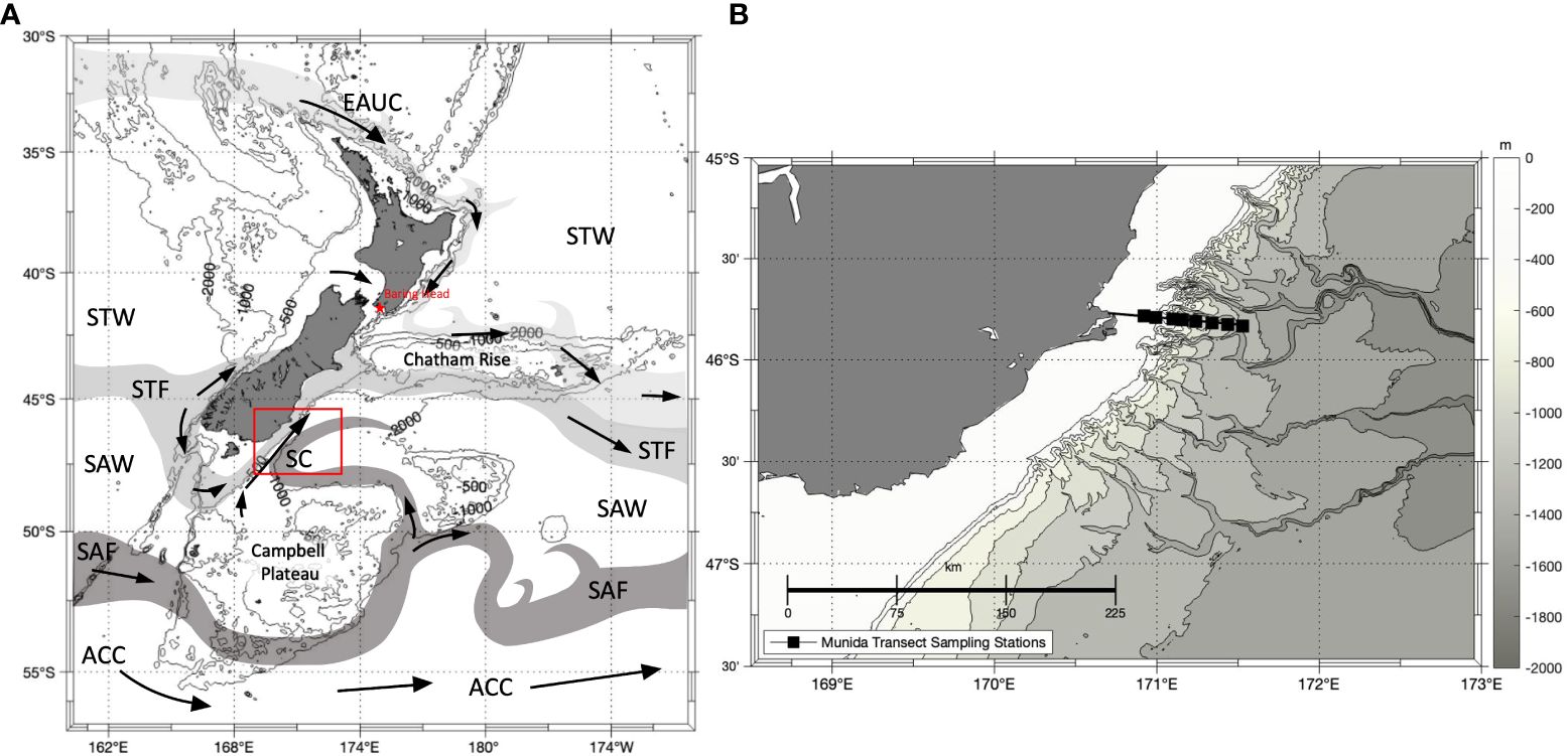
Figure 1 (A) Map of major fronts, surface currents and water masses, and topographical features around New Zealand (adapted from Chiswell et al., 2015) including subtropical water (STW), the Subtropical Front (STF), subantarctic water (SAW), Subantarctic Front (SAF), the East Auckland Current [EAUC, an extension of the East Australian Current, EAC and the Tasman Front (not labeled)], the Southland Current (SC), and the Antarctic Circumpolar Current (ACC). Transport along major fronts are color coded from lighter to darker corresponding to warmest to coolest. Red start indicates location of Baring Head where atmospheric CO2 samples used in this study were collected. Red box indicates the study domain shown in (B) Map showing the study domain off the Southeast coast of New Zealand. Black line shows the Munida Time Series transect with black boxes indicating sampling stations. Bathymetry is given by greyscale contours.
The South Island lies in the convergences zone within the Southern Ocean, where the high macronutrient low chlorophyll waters of the subantarctic (SAW) meet the oligotrophic subtropical (STW) waters fueling primary productivity (Safi et al., 2023). The coastal margins of New Zealand are dominated by the South Pacific WBC system (See Figure 1A), which has been shown to be warming, intensifying, and shifting poleward in recent years (Li et al., 2022). Li et al. (2022) showed a very strong correlation between the Southern Annular Mode (SAM) and the position of zero wind stress curl across the South Pacific. This increasing trend in positive SAM is driving the easterlies south, which is correlated with warming, intensification, and the poleward migration of the East Australian Current (EAC), the WBC of the South Pacific (Li et al., 2022). The Southland Current (SC) is a dominant regional feature (~10 Sv) that bisects the MTS. Unlike other WBC extensions, the SC flows northward along the STF off the southeast coast of the South Island (Sutton, 2003; Fernandez et al., 2018). Modelling studies indicate regional topography is critical to driving the SC, which uniquely flows counter to Sverdrup balance with two feeding pathways. The shallow pathway approaches from the southwest of the South Island following gradients in sea surface height (Tilburg et al., 2002; Hurlburt et al., 2008). The deep pathway in which the SAF forms a deep water boundary current along the Campbell Plateau that passes through a gap around 48°S, is constrained by a sill and topographically steered eastward toward the South Island where it turns northeast joining the shallow pathway (Tilburg et al., 2002; Hurlburt et al., 2008). Interactions between the Antarctic Circumpolar Current (ACC) and regional topographic features influence the distribution of water masses, including mode water, and also circulation patterns, which are important to the surface carbon cycle around New Zealand (Chiswell et al., 2015). Given the changes in the WBC system and the sensitivity of the Southern Ocean to climate change, it is important to understand the connection between climate change, ocean basin scale variability, and regional variability along the coastal margins of New Zealand (Morley et al., 2020).
Although seasonal variability in surface layer DIC in the subantarctic surface waters has been established in the MTS by Brix et al., 2013, that study did not characterize the interannual variability, nor address long-term trends in the processes controlling the DIC concentration. However, Brix et al. did report a divergence between trends in surface ocean pCO2 and that expected from anthropogenic emissions, but were unable to explain this disequilibrium at the time. Techniques subsequently established by Fassbender et al. (2016) enable deconvolution of net community production and carbonate production within the biological processes term of the DIC budget, which were not previously evaluated in the MTS. We hypothesize that advection plays a more important role than previously reported by Brix et al. (2013) via transport of water with higher DIC concentrations into the region. An additional decade of observations since the Brix et al. study (2013), now enables assessment of the drivers of variability in the regional carbon cycle over seasonal to decadal time scales, and improved characterization of the disequilibrium between ocean and atmosphere pCO2. MTS observations were combined with remote sensing and reanalysis data to evaluate the regional carbon budget. We apply a mass balance box model to deconvolve the seasonal carbon cycle in the surface mixed layer. Using ocean transport and meteorological data we constrain the physical terms in the carbon budget and estimate the biologically fixed carbon available for export from the surface ocean. Nutrient stoichiometry was also used to estimate biological production, based on changes in phosphate concentration, and compared to the carbon budget residual approach of Fassbender et al. (2016, 2017). Using these methods, we assessed variability in the biological pump, solubility, and the physical transport of carbon over climatically relevant timescales.
2 Materials and methods
2.1 Hydrographic, satellite and reanalysis datasets
Several ancillary data sets were used with MTS observational data to interpolate the observations through time and spatially extrapolate them for assessment of the regional carbon cycle. Remotely sensed and reanalysis data were gathered for the domain surrounding the MTS shown in Figure 1. Table 1 provides details for all datasets used in this analysis.
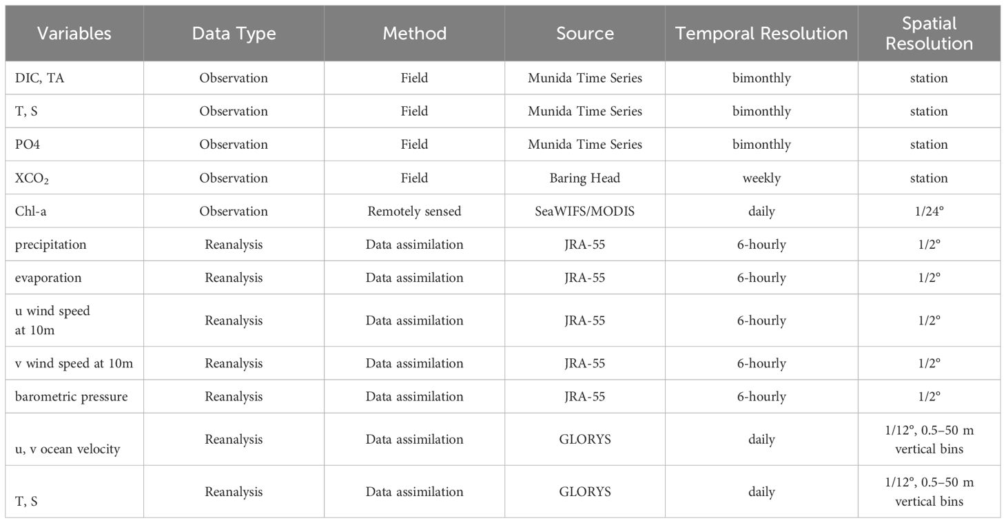
Table 1 Variables with associated type, method, source, and spatiotemporal resolutions for the datasets used in this this carbon budget evaluation.
2.1.1 Munida Time Series
There are 8 sampling stations along the Munida transect (see Figure 1B). CTD casts and bottle sampling for TA, DIC, chlorophyll a, nitrate, phosphate, and silicate concentrations, are routinely collected (every two months) at the end of the line in the SAW, and intermittently sampled at the other stations along the transect, while pCO2, temperature, and salinity are measured continuously along the entire surface transect. Surface samples are collected at approximately 2m depths while profiles are captured with samples collected using niskin bottles at depths of 50m, 100m, 200m, and 500m (Currie et al., 2011b). Here we use the time series of observations collected in the SAW to evaluate the seasonal to long term variability in the surface layer carbon budget, while utilizing measurements made along the entire transect for estimating regional surface layer DIC to establish gradients and estimate physical transport terms.
MTS samples are processed at the NIWA/University of Otago Research Centre for Oceanography laboratory. DIC is measured coulometrically with an accuracy< 2.0 μmol kg-1 based on certified reference materials (CRD) (Dickson et al., 2007). TA is analyzed by automated potentiometric titration and derived using a least squares optimization technique with an accuracy of<1.0 μmol kg-1 based on CRMs (Dickson et al., 2007; Currie et al., 2011a), Nutrients are analyzed colourimetrically and the uncertainty of phosphate (PO4) measurements is 0.1 μmol kg-1 (Currie et al., 2011b; Jones et al., 2013).
2.1.2 Remotely sensed chlorophyll
Monthly composites of satellite-derived chlorophyll data (O’Reilly et al., 1998) from MODIS (2003 – 2018) and SeaWIFS (1998 – 2002) (O’Reilly et al., 1998) were paired with observations for training multiple linear regression (MLR) models using the mean surface chlorophyll calculated from the 20 km2 surrounding each sampling station. Mean bias for MODIS derived chlorophyll surrounding New Zealand is 1.16 mg m-3 (Bailey and Werdell, 2006).
2.1.3 Reanalysis data products
The Mercator Ocean Global Reanalysis (GLORYS) has been demonstrated to show effectively simulate physical properties of surface waters surrounding New Zealand (de Souza et al., 2020). GLORYS uses the NEMO ocean model with LIM3 sea ice model and assimilates sea level anomaly observations, sea surface temperatures and in situ temperature and salinity, as well as sea ice concentration (Lellouche et al., 2023a). Mean temperature bias is 0.08°C (warmer); mean salinity bias is 0.02 psu (fresher); mean surface current error for the study region is 0.01 – 0.06 m/s (Lellouche et al., 2023a).
GLORYS physical data (T, S, u, v, w) was averaged over a 20 km2 box surrounding the MTS while the regional gradients were established using domain-wide data. Comparisons between GLORYS and MTS temperature and salinity in the mixed layer are provided in the Supplementary Materials (Supplementary Figure S3) and the RMSE values are discussed in Section 2.4 below. For internal consistency in this analysis, GLORYS temperature and salinity are used instead of MTS observations. Given that GLORYS assimilates available temperature and salinity data, it may provide a better representation of variability over interannual to decadal time scales.
The Japanese 55-year Reanalysis (JRA-55) was used for meteorological values of wind, precipitation, evaporation, and barometric pressure (Onogi et al., 2007; Kobayashi et al., 2015) in conjunction with atmospheric CO2 measurements from Baring Head, New Zealand (Cox et al., 2021) in the calculation of air-sea CO2 flux, surface freshwater flux, and wind driven circulation in the surface layer. JRA-55 precipitation data was shown to generally outperform other reanalysis data products in a temperate climate study (Odon et al., 2019), and JRA-55 winds also compare well with oceanic observations with some biasing related to ENSO (Wen et al., 2018). Uncertainty in the measurement of atmospheric CO2 using discrete samples is < 0.2 ppm (Thoning et al., 1989; Lan et al., 2022).
2.2 Time series imputation and spatial extrapolation
The sampling frequency in the MTS is approximately bimonthly, with variable months sampled year-to-year. The time series must be imputed to monthly sampling to optimally assess interannual variability (IAV); however, it is important that gap-filling methods maintain the natural variability and long-term trends. Vance et al. (2022) recently identified that an empirical multiple linear regression (MLR) model that estimates DIC from remotely observed chlorophyll concentrations, sea surface temperature and salinity provided the most robust approach to imputing missing data compared to other common statistical and empirical methods. This MLR can be augmented to further improve the representation of interannual variability by adding terms for time variance. Here we changed the chlorophyll predictor to a logarithmic relation based on the relative concentrations and added harmonic functions in Equation 1 to describe seasonal variability and a yearly term to account for long-term trends.
where C is the concentration of the variable (e.g. DIC), T is temperature, S is salinity, mo is month, yr is year, the subscript a indicates the mean surface layer concentration and and are model coefficients. When fitting this MLR with SAW data alone, Equation 1 estimates DIC with an RMSE of 6.91 μmol kg-1. This imputation approach was used to generate a continuous monthly time series for the MTS.
Surface layer TA and PO4 from the MTS were imputed to obtain a monthly time series using Multiple Imputation by Chained Equations (MICE) using the mice package in R version 3.5.2 (R Core Team, 2020), with the function call mice(data = timeseries$data, m = 5, method = pmm, maxit = 50), where m is the number of multiple imputations, method is predictive mean matching, and maxit is the maximum number of iterations. Using MICE, missing values are first filled by random sampling from observations for the imputation variable (TA). Then the first variable is regressed against all other variables using only observed values. This methods is designed to impute multiple variables and then iteratively fit regression models for remaining variables (White et al., 2011). For each imputation point it estimates m times and provide estimates. The mean of these model solutions is taken as the imputation value and the standard deviation as the uncertainty. The mean uncertainty for all imputations was 4.61 μmol kg-1 for TA and 0.05 μmol kg-1for PO4 (See Supplementary Material and Vance et al., 2022 for additional details).
The MLR in Equation 1 was also fitted using data along the full surface MTS transect across the inner shelf to the shelf break to produce model coefficients applicable to all water regional masses for spatial extrapolation using remotely sensed chlorophyll and ocean reanalysis data. This domain-wide MLR predicts DIC over the salinity range 33–35 psu with an RMSE of 12.15 μmol kg-1 (See Supplementary Figure S3). This domain-wide MLR was similarly applied to TA (RMSE = 7.79 μmol kg-1). This MLR was applied from 48°S, 169°E to 45°S, 174°E for estimating horizontal concentration gradients in DIC and TA to inform the advection term in the surface layer carbon budget.
The vertical gradients of DIC and TA are required to evaluate the effects of entrainment and vertical mixing by eddy diffusivity on the surface layer concentrations. Available profiles of DIC, TA, and PO4 (2012 - 2017) were used to develop the MLR in Equation 2 to estimate the vertical concentration gradients at the base of the mixed layer.
where the subscript z indicates the value at depth of 20m below the mixed layer, h is the mixed layer depth (MLD), and and are model coefficients. This MLR predicts subpycnal DIC with an RMSE of 1.08 μmol kg-1; subpycnal TA with an RMSE of 1.44 μmol kg-1; and subpycnal PO4 with an RMSE of 0.02 μmol kg-1 (see Supplementary Figure S6 in Supplementary Material).
2.3 Surface layer carbon budget
Seasonal variability in the ocean carbonate system is driven by physical and biological processes that vary across disparate water masses, frontal regions, and ecosystem types. To assess the drivers of variability in DIC across the subtropical frontal zone, a mass balance budget of DIC in the mixed layer was evaluated that accounted for changes resulting from the linear combination of air-sea CO2 exchange (Air-Sea), physical transport (Phys), freshwater flux due to evaporation/precipitation differences (E-P), net community production (NCP) and inorganic carbonate production (CaCO3):
In situ MTS observations were used along with physical and meteorological reanalysis data to evaluate the budget terms over the years 1998 - 2022. The same approach was also applied to evaluate the surface alkalinity budget (Equation 2), but without the air-sea term as CO2 exchange does not affect alkalinity.
The physical term in Equations 3 and 4 contains horizontal advection, entrainment, and horizontal and vertical mixing due to eddy diffusivity as described in Equation 5 (Vijith et al., 2020):
where C is the concentration of the variable (e.g. DIC, TA) the subscript a denotes vertically averaged values in the mixed layer (h), while the subscript h denotes values at the base of the mixed layer and u is the vertically averaged horizontal velocity, is the gradient operator, and w are the zonal, meridional, and vertical velocities respectively, and are the horizontal and vertical eddy diffusivity coefficients respectively.
The vertical velocity at the base of the mixed layer was estimated from the Sverdrup balance (Equation 6) with the assumption that the turbulent stress diminishes at the base of the mixed layer as in Cronin et al. (2013):
where is the acceleration due to gravity, is the Coriolis parameter, is the meridional gradient in , is the sea surface height, is the wind stress and is the zonal component of the wind stress. The horizontal eddy diffusivity coefficient (Equation 7) was estimated from the length scale according to (Okubo, 1971):
where L was set to 150 km to account for mesoscale dynamics along the frontal region. The vertical eddy diffusivity coefficient (Equation 8) was estimated from the mixing efficiency [Γ = 0.2, constant per Gregg et al. (2018)], the turbulent kinetic energy dissipation rate (ε) and the Brunt-Vaisala frequency ():
where ε is estimated from the velocity shear and the viscosity as in Equation 9:
The influence of the surface freshwater flux on mixed layer DIC and TA was estimated from the salinity mass balance change arising from the effects of evaporation and precipitation. The freshwater balance from JRA-55 evaporation (E) and precipitation (P) data was applied to the mean ratios of DIC and TA to salinity at the air-sea surface (depth = 0m) according to Equation 10:
Air-sea CO2 exchange was estimated from air-sea CO2 gradient (), the solubility of CO2, and the gas transfer velocity as in Equations 11, 12:
where
and is the temperature-, salinity- and pressure-dependent solubility of CO2 in seawater (Weiss, 1974), and is the vertically averaged density within the mixed layer, h, and k is the gas transfer velocity calculated from JRA-55 wind speed at 10 m (Equation 13) according to Ho et al. (2006), which was derived near the MTS for use in the Southern Ocean region:
Where Sc is the Schmidt number and is the wind speed at 10 m above the mean sea level. Atmospheric CO2 was converted from mole fraction in dry air (XCO2) to partial pressure of CO2 using Equations 14 and 15, accounting for the barometric pressure and the effects of water vapor in the atmosphere.
where T is the temperature (in Kelvin), S is the salinity at the air-sea surface, and is the barometric pressure at mean sea level. Surface ocean pCO2 was calculated based on the mixed layer concentrations of DIC and TA using the R package seacarb (Gattuso et al., 2012; Orr et al., 2018) with K1 and K2 from Lueker et al. (2000), Kf from Dickson (1979), and Ks from Dickson et al. (1990).
With physical transport, freshwater flux, and gas exchange budget terms estimated from reanalysis data (where reanalyses include assimilated observations), the biological processes that influence DIC and TA can be estimated as a residual of the budget, as in Fassbender et al. (2016). Calcification decreases DIC and TA in a 1:2 ratio for each mol of CaCO3 precipitated, whereas primary production of organic matter consumes 117 mol CO2 and 18 mol H+, increasing TA by 17 mol for each mol of PO4 utilized (Sarmiento and Gruber, 2006). This stoichiometry can then be used to solve the following set of equations (Equations 16–18) to estimate the NCP and calcification terms:
where R denotes the residual of the respective DIC and TA budgets.
2.4 Uncertainty and limitations
Overall uncertainty was assessed by first accounting for measurement uncertainty, uncertainty in averaging monthly means, time series imputation and spatial extrapolation, and then propagating errors through calculations in the budget evaluation. These uncertainties are presented in Table 2. In cases where interpolated values have been used, uncertainty was taken as the cross-validated RMSE of regression models. The RMSEs between GLORYS temperature and salinity values and MTS observations were applied. Estimated uncertainties of reanalysis data products were used for parameters not measured with the MTS based on prior validation studies (Jean-Michel et al., 2021). For surface gradients (DIC and TA) the RMSE for the concentration estimation using the MLR in Equation 1 was added in quadrature with standard deviation across the domain to estimate the combined uncertainty.
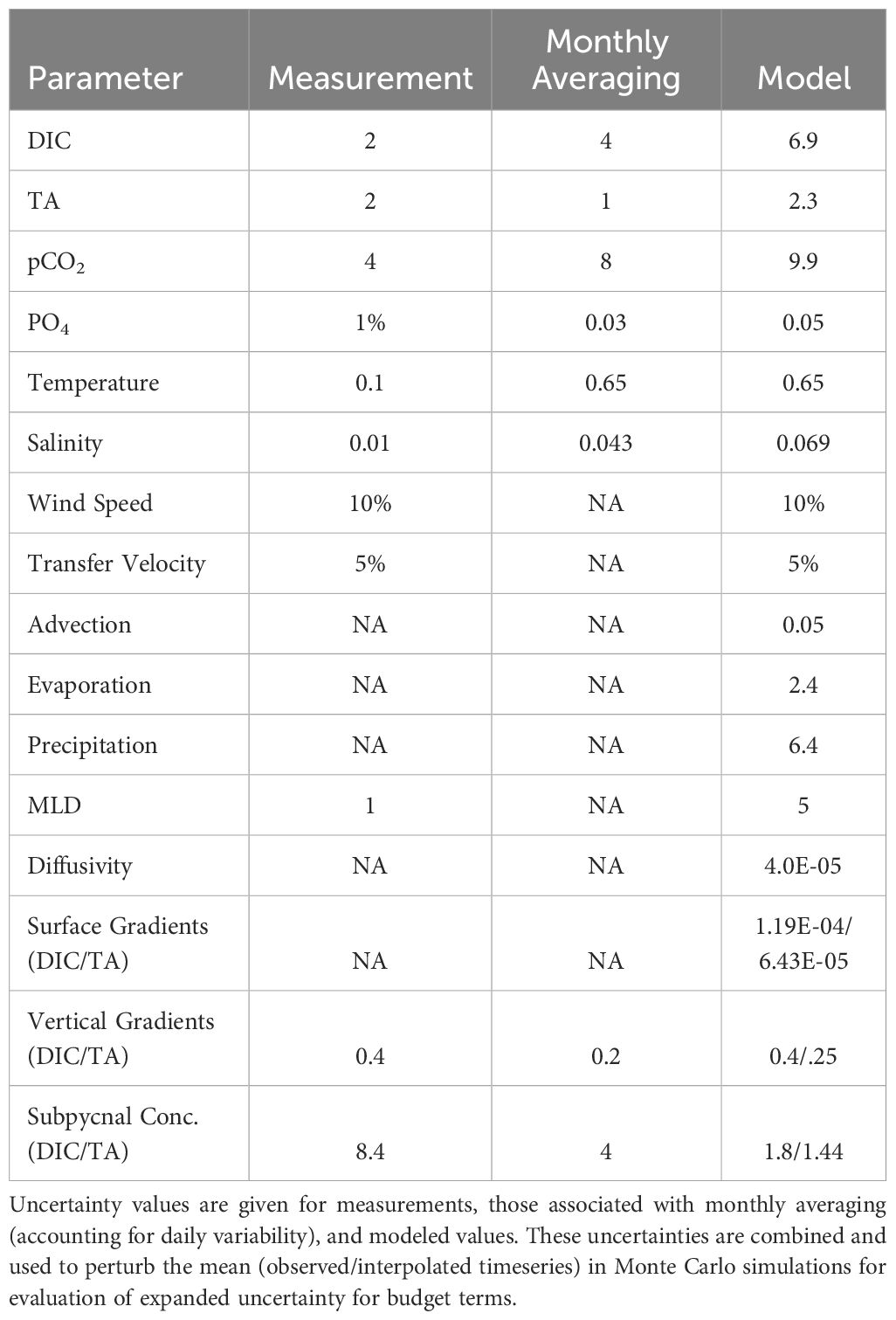
Table 2 Uncertainty values associated with each parameter in the DIC and TA budgets.
A Monte Carlo approach was used to account for covariance and nonlinear relationships in the budget calculations. For each term in the surface DIC and TA budgets (Equations 1, 2 above), input timeseries used for the calculations were randomly perturbed away from the mean (monthly observations and interpolated timeseries values) by the uncertainties listed in Table 2. 1000 simulations were run for each budget term using gaussian distributions and the expanded uncertainty for each data point in the timeseries for each budget term was estimated as the 95% confidence interval (CI).
There are several assumptions and limitations to consider for the methods developed for this analysis. Firstly, it is assumed that the imputation methods do not significantly bias the interannual variability and long-term trends in the DIC and TA timeseries. This is reasonable given the performance of a similar empirical MLR (Equation 1) and MICE for the MTS and other ocean carbon time series (Vance et al., 2022). It is assumed that the MLR coefficients (See Supplementary Table S1 for MLR coefficients) for DIC and TA applied to the STW and SAW along the Munida transect are consistent for these water masses within the domain. The GLORYS temperature and salinity profiles compare well with observations and help to constrain the estimates of vertical DIC and TA gradients at the base of the mixed; however, the relative uncertainty of this term is larger than others in the budget.
Care must be taken when considering the precipitation and evaporation reanalysis data, which can have large relative uncertainties; however, it was anticipated that this balance would have a small influence over the seasonal cycle and interannual variability. While JRA-55 wind reanalysis performs well compared to the Tropical Atmosphere Ocean observations (Wen et al., 2018), biasing due to ENSO variability will propagate into air-sea flux estimates. Advection terms from the GLORYS reanalysis data exhibit greater divergence in coastal environments where submesoscale processes and terrestrial river influences are not represented and data assimilation is sparse (Lellouche et al., 2023b). However, the SAW, which is the focus in this study, is located at and beyond the shelf break where these divergences are minimized. Processes controlling variability in the surface layer carbonate chemistry can only be inferred with an adequate signal to noise ratio.
3 Results
The results of this study are presented starting with the observed seasonal profiles and interpolated time series used to evaluate the terms in the surface DIC and TA budgets. Next, the seasonal climatologies of the processes controlling the DIC and TA cycles. Then, the annually integrated budget terms are presented with an evaluation of the interannual variability. Following that, the monthly budget source terms are vertically integrated through the mixed layer and long-term trends are evaluated for the MTS. Lastly, decadal variability and shifts in trends in carbonate parameters and controlling factors are presented.
3.1 Climatological carbon cycle
Monthly climatologies of DIC profiles in SAW from 0 – 500 m constructed from in situ MTS illustrate the seasonal cycle in the surface layer, with stronger vertical gradients associated with seasonal stratification and draw down of DIC during Austral summer, whereas DIC at 500 m shows little seasonal variability (Figure 2). Thermal stratification as the MLD shoals in the autumn precedes the biological draw down in summer. Error bars illustrate greater variability in the mixed layer than at lower depths; however, some of the differences across months is due to sampling bias.
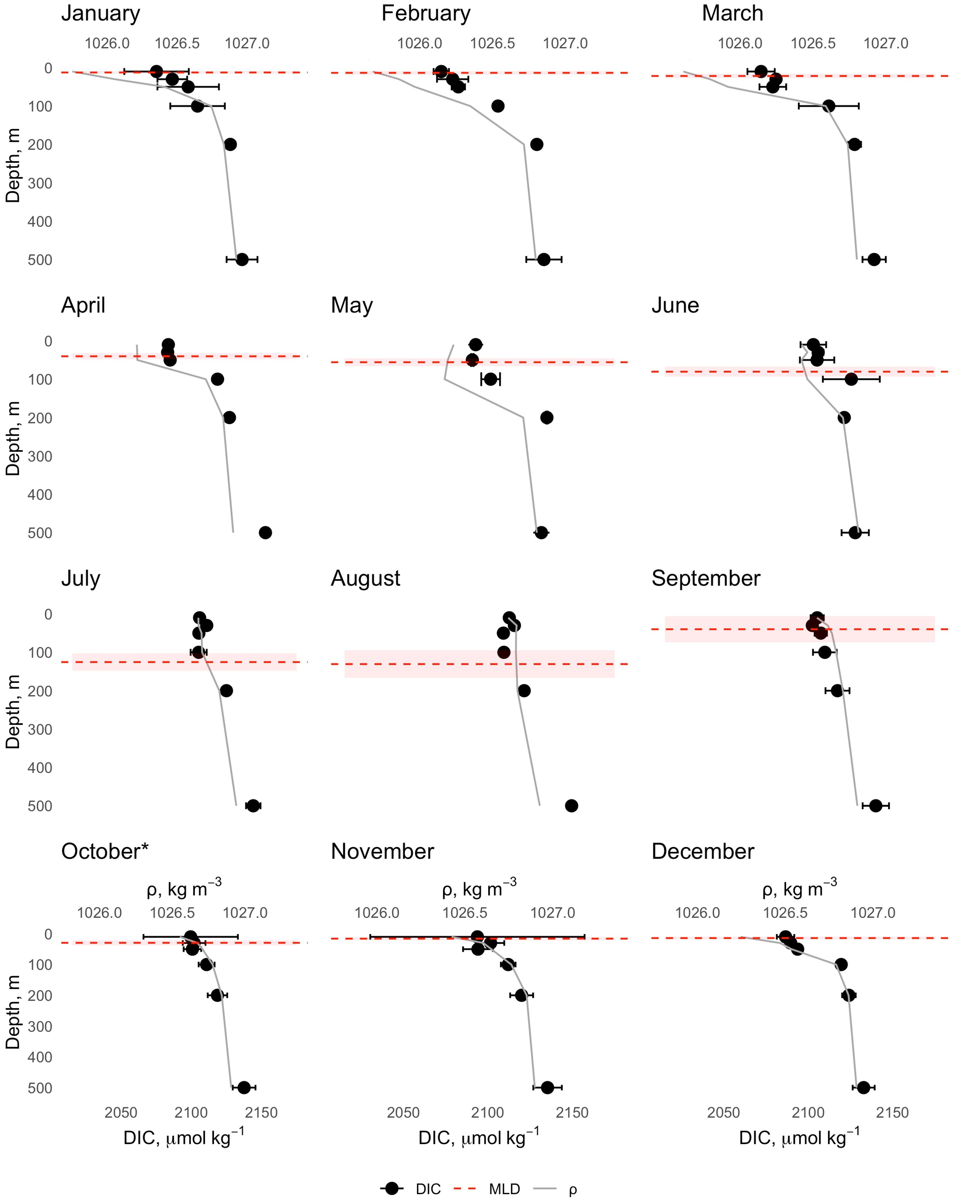
Figure 2 Monthly climatologies of MTS DIC profiles (black) with errors bars representing the standard deviation of the monthly means. Mixed layer depth is given by the red dashed line with the red ribbon indicating the standard deviation of the monthly mean and density profiles determined from Munida CTD are shown in grey.
The uncertainty of the imputed time series of SAW mixed layer DIC, TA, phosphate concentration, temperature, and salinity used to evaluate the inorganic carbon budget is consistent with the measurement uncertainty (Figure 3). While there is divergence between the GLORYS salinity and that measured by the MTS, the variability is consistent between them supporting the use of GLORYS for the budget evaluation. The timeseries of subpycnal DIC and TA generated using the MLR in Equation 2 is consistent with the observations, with the TA showing somewhat larger variability (Figure 4). The trend in subpycnal DIC appears larger than in the surface layer DIC (0.45 μmol kg-1 y-1 vs. μmol 0.25 kg-1 m-1 respectively); however, this is consistent with regional trends in water masses derived from float data (Mazloff et al., 2023).
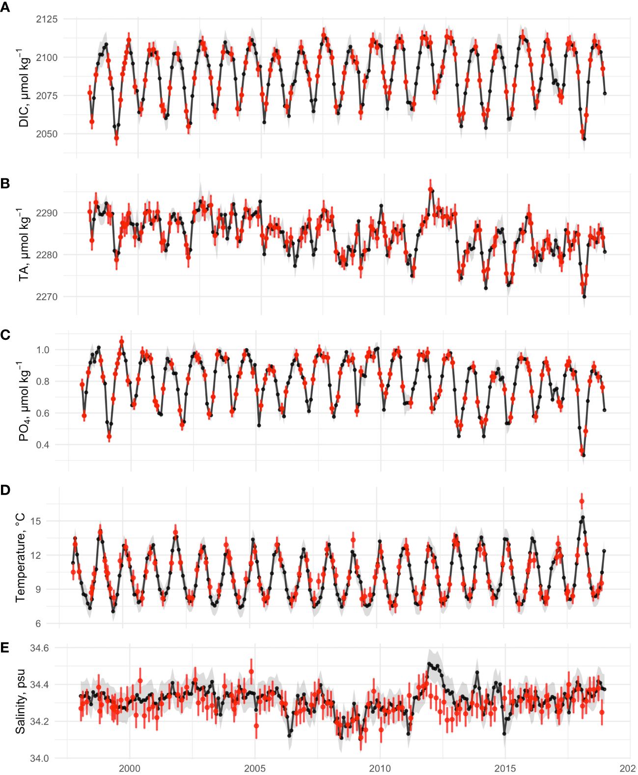
Figure 3 Imputed time series (black, 1998–2018) of mixed layer (A) DIC, (B) TA, (C) phosphate, (D) temperature, and (E) salinity at the MTS with observations overlaid (red markers). Note temperature and salinity (black) time series were produced from GLORYS.
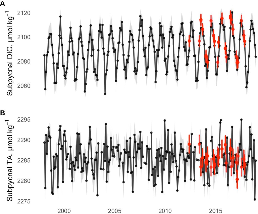
Figure 4 Time series (black, 1998–2018) of estimated of subpycnal layer concentrations of (A) DIC, and (B) TA, in the MTS with observations overlaid (red markers).
The 20-year seasonal climatology of the deconvolved carbon cycle is shown in Figure 5 as monthly rates of change (see Supplementary Figures S7, S8 for corresponding monthly timeseries). The tendency (observed rate of change) and the contribution of each budget term was evaluated by fitting a local polynomial regression (LOESS) of the seasonal cycles for all years of the time series (Hastie et al., 2018). The mean and seasonal maxima and minima for each process are provided in Table 3. The uncertainty of the climatology was fit using LOESS of uncertainties for each timeseries data point that were evaluated as the 95% CI of 1000 Monte Carlo simulations as described above. The climatology in Figure 5 shows a strong influence of horizontal advection, which makes the largest contribution to change in DIC, adding a mean 12.40 ± 0.77 μmol kg-1 m-1. Peak DIC advection occurs during late austral summer (Jan-Feb) with a seasonal maximum rate of 25.56 ± 0.77 μmol kg-1 m-1 driven by strong surface gradients, which weakens to 3.80 ± 0.77 μmol kg-1 m-1 during austral winter when concentrations are high across the region and surface gradients are weakest. Surface gradients in TA are strong zonally across the subtropical front (see Supplementary Figure S5), while the meridional gradients along the mean flow of the Southland Current are weak. The orientation of the gradients relative to the mean geostrophic flow that dominates the transport results in smaller advective transport terms for TA (5.07 ± 0.40 μmol kg-1 m-1) relative to DIC along the Otago shelf.
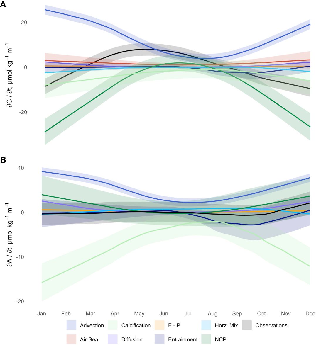
Figure 5 Mean seasonal climatology of deconvolved carbon cycle at the MTS with the observed monthly rate of change (tendency, black) and biological processes (net community production (NCP), dark green; and calcification, light green) for DIC (A) and TA (B) also with the monthly rates of change due to physical processes (air-sea gas exchange, red (DIC only); evaporation-precipitation balance (E-P), orange; horizontal advection, dark blue; horizontal mixing, light blue; diffusion at the base of the mixed layer (vertical mixing), purple, and entrainment, navy). Solid lines indicate mean rates of change over seasonal cycle as determined by LOESS fits over the 20-year observations for each process. Ribbons indicate 95% CI about the means. See Equations 1-3 for definition of terms.
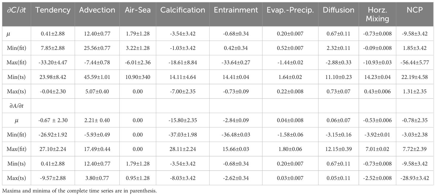
Table 3 Statistics of the seasonal fitted monthly rates of change associated with each budget term (see Equations 1-3 for definitions) including the means (μ), standard deviations (σ), minima, and maxima with units in μmol kg-1 m-1.
Horizontal mixing reduces DIC at a mean rate of 0.73 ± 0.008 μmol kg-1 m-1 while adding a mean 0.43 ± 0.006 μmol kg-1 m-1 TA. Horizontal mixing reaches a maximum rate of 2.52 ± 0.008 DIC μmol kg-1 m-1 and 0.91 ± 0.006 TA μmol kg-1 m-1 in summer. Diffusive fluxes are influenced by stratification and peak in the summer when the vertical gradients across the base of the mixed layer are strongest, adding DIC and TA to the mixed layer from the subpycnal layer below at mean rates of 0.67 ± 0.11 μmol kg-1 m-1 and 0.73 ± 0.07 μmol kg-1 m-1 respectively. The vertical entrainment term accounts for seasonal changes in the MLD due to changes in density, as well as vertical advection at the base of the mixed layer due to surface wind stress (Ekman pumping) and lateral induction, which occurs due to advection across a sloping mixed layer base; consequently, in our model the entrainment term adds and removes DIC from the surface layer, as in the salinity budget evaluations of Vijith et al. (2020). Vertical entrainment reduces the DIC and TA by mean rates of 0.68 ± 0.34 μmol kg-1 m-1 and 0.73 ±0.09 μmol kg-1 m-1 respectively as the MLD shoals in this downwelling dominant system (Stevens et al., 2019). The E-P flux has the smallest impact on the seasonal carbon cycle. Net evaporation in the E-P balance during summer drives a mean increase of 0.2 ± 0.02 μmol kg-1 m-1 in DIC and TA. The air-sea gas exchange term indicates that this region is a net sink for atmospheric CO2 with a mean rate of 1.79 ± 1.28 μmol kg-1 m-1 of DIC per year and a seasonal maximum rate of 3.22 ± 1.67 μmol kg-1 m-1. Absolute maxima and minima values for each budget term in the time series are also provided in Table 3 and shown in Supplementary Figures S9, 10 in the Supplementary Material.
DIC added through air-sea exchange and advection is balanced by biological activity. Net community production and calcification both exhibit peak carbon drawdown in summer. NCP reduces DIC in the surface layer by a mean rate of 9.58 ± 3.42 μmol kg-1 m-1 with a seasonal maximum rate of 28.93 ± 3.42 μmol kg-1 m-1, while calcification reduces DIC at a mean rate of 3.56 ± 3.42 μmol kg-1 m-1 with a seasonal maximum rate of 8.03 ± 3.42 μmol kg-1 m-1. NCP has an opposing effect on TA with a mean rate of 13.19 ± 2.35 μmol kg-1 m-1 and a seasonal maximum of 4.79 ± 2.35 μmol kg-1 m-1, whereas calcification reduces TA at a mean rate of 7.00 ± 2.35 μmol kg-1 m-1with a seasonal maximum of 15.80 ± 2.35 μmol kg-1 m-1.
The seasonal net community production estimates based on observed PO4 concentrations and Redfield stoichiometry [106 mol of carbon consumed for every mol PO4 during organic matter production (Sarmiento and Gruber, 2006)] are consistent using these two approaches, although the PO4 derived values indicate a weaker biological pump (See Supplementary Figure S11 and Section 4.1 for additional details).
3.2 Seasonal integration and interannual variability
Monthly rates of change in mixed layer DIC and TA were integrated through time from the start of each year in the time series to provide cumulative ΔDIC and ΔTA values for each budget term. The changes in DIC and TA resulting from each budget term were used to calculate the corresponding change in pCO2. The effect of changes in water temperature on pCO2 were also calculated and included as a pCO2-specific budget term. The statistics of these cumulative ΔDIC, ΔTA, and ΔpCO2 are summarized in Table 4. Interannual variability (IAV) here is defined as the standard deviation (σ in Table 4) across the 20-year timeseries in the cumulative change in mixed layer DIC, TA, or pCO2 resulting from each budget term. See Supplementary Figure S13 for the mean (LOESS fit) for the cumulative ΔDIC, ΔTA and ΔpCO2 for each budget term with color coded years to illustrate the IAV. The uncertainty of the seasonally integrated changes was evaluated by adding the uncertainty for each monthly term value in quadrature for each year, and then averaging for the mean annual values, resulting in higher uncertainty values than those associated with the MCM and LOESS fitting in the climatology above. The uncertainty in ΔpCO2 was evaluated by adding the change in pCO2 associated with the uncertainties in ΔDIC and ΔTA, with the error estimated using the errors function within the R package seacarb (Jean-Pierre Gattuso et al., 2012; Orr et al., 2018) in quadrature.
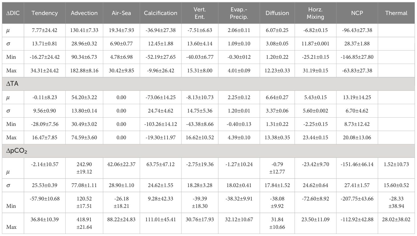
Table 4 Statistics of the annual cumulative change associated with each DIC and TA budget term and the corresponding changes in pCO2, including the mean (μ), standard deviation (σ), minimum, and maximum, with DIC and TA in units of μmol kg-1 and pCO2 in units of μatm.
Table 4 shows that advection and NCP make the greatest contribution to DIC and pCO2 IAV (54% and 59% respectively). These processes account for 26% of TA IAV while calcification is the single most significant process for TA IAV, at nearly 37% (Table 4). Vertical entrainment contributes 13% and 22% to DIC and TA respectively but only 1% to pCO2 IAV. Horizontal mixing contributes 8% to TA and pCO2 IAV and 11% to DIC IAV. The freshwater balance has minor impact on IAV, contributing< 1% to DIC, TA, and pCO2 IAV, and thermal effects on pCO2 contribute 9% to IAV.
3.3 Annual fluxes and long-term variability
Rates of change were integrated through the mixed layer to evaluate the monthly carbon source terms (J) in units of mol C m-2 y-1. Monthly DIC source contributions were then deseasoned and linearly regressed through time to evaluate long term trends for each physical and biological process. Figure 6 shows the monthly carbon source contributions for each term with annual means indicated by red markers and regression slopes as dashed lines. Note that positive values indicate fluxes into the surface layer. Significant trends were found for air-sea flux (0.026 ± 0.006 mol C m-2 y-2), advection (-0.107 ± 0.045 mol C m-2 y-2), and horizontal mixing (0.061 ± 0.018 mol C m-2 y-2) terms. Diffusive and freshwater fluxes were very close to the 0.05 p-value threshold for significance (p > 0.06), with diffusive fluxes increasing at a rate of 0.004 ± 0.002 mol C m-2 y-2 and freshwater fluxes decreasing at a rate of -0.002 ± 0.001 mol C m-2 y-2. NCP and calcification do not show any trend in annual fluxes, despite a long-term trend in remotely sensed chlorophyll of 0.003 ± 0.0009 mg m-3 y-1 (see Supplementary Figure S12).
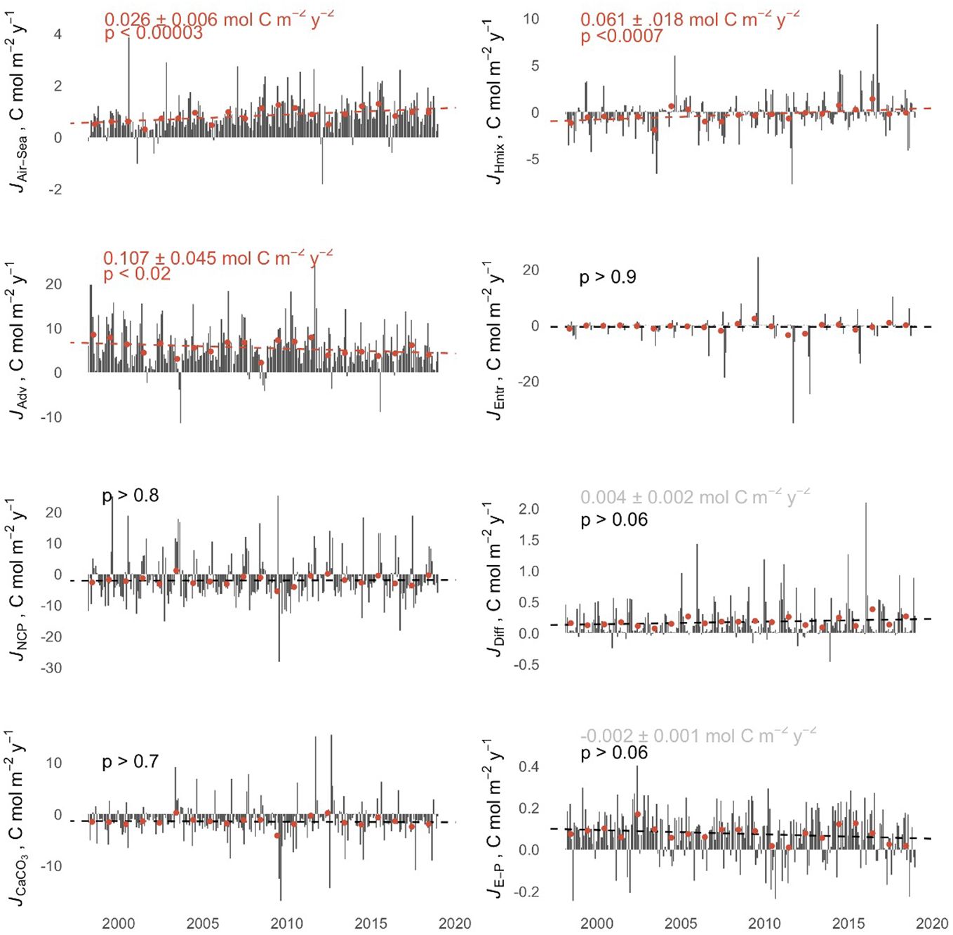
Figure 6 Monthly (grey bars) and annual (red symbols) fluxes for each term in the carbon budget integrated through the mixed layer. Positive values indicate fluxes into the surface layer. Trend assessments with uncertainty and p-values are shown where significant (red text, air-sea flux, advection and horizontal mixing) and also when close to a threshold of p< 0.05 (grey text, diffusion and freshwater flux). Note the y-axes are scaled independently for each process to maximize visualization of interannual and decadal variability.
Table 5 shows the summary statistics for the annual carbon fluxes associated with each budget term. Advection represents the largest surface layer flux of DIC in the annual carbon cycle followed by NCP, calcification, air-sea flux, vertical entrainment, horizontal mixing, diffusion and freshwater flux in descending order.
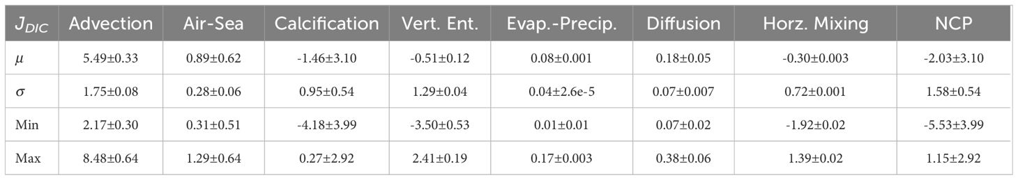
Table 5 Statistics of annual fluxes (J) associated with each carbon budget term integrated through the mixed layer depth, including the mean (μ), standard deviation (σ), minimum, and maximum, with units of mol C m-2 y-1.
Acidification of SAW at the MTS has occurred concurrently with increasing pCO2 since 1998 (Bates et al., 2014). However, the time series indicates shifting trends over decadal time scales. Multiple methods of change point detection were applied in this study (PELT, CUSUM, BCP, Segmented, and Tree), and all detected a shift in the time series during 2009–2010 (see Supplementary Figures S15-S19 in Section 5). This was the case for both pCO2 calculated from interpolated DIC and TA measurements and surface pCO2 measured in situ (see Supplementary Figure S20). The small change in the decadal trend in atmospheric pCO2 is consistent with the increase in global carbon emissions over these time scales (Friedlingstein et al., 2022). During 1998 – 2010 surface ocean pCO2 at the MTS increased at a rate that was less than one third of that in the atmosphere, suggesting regional biological and physical processes influenced the surface pCO2 trend since the equilibration time scale for air-sea gas exchange is on the order of months. Whereas ΔpCO2 increased by 1.29 ± 0.04 μatm y-1 during 1998 – 2010 (see Figure 7) a significant shift occurred during 2010 – 2018, with no significant trend but instead consistent interannual variability, indicating the ocean was equilibrating with rising atmospheric CO2 during this period. Whereas the trend in atmospheric pCO2 in 2010 – 2018 was 26% higher than in the previous decade, the ocean trend was 322% higher, indicating a substantial change in the processes controlling ΔpCO2.
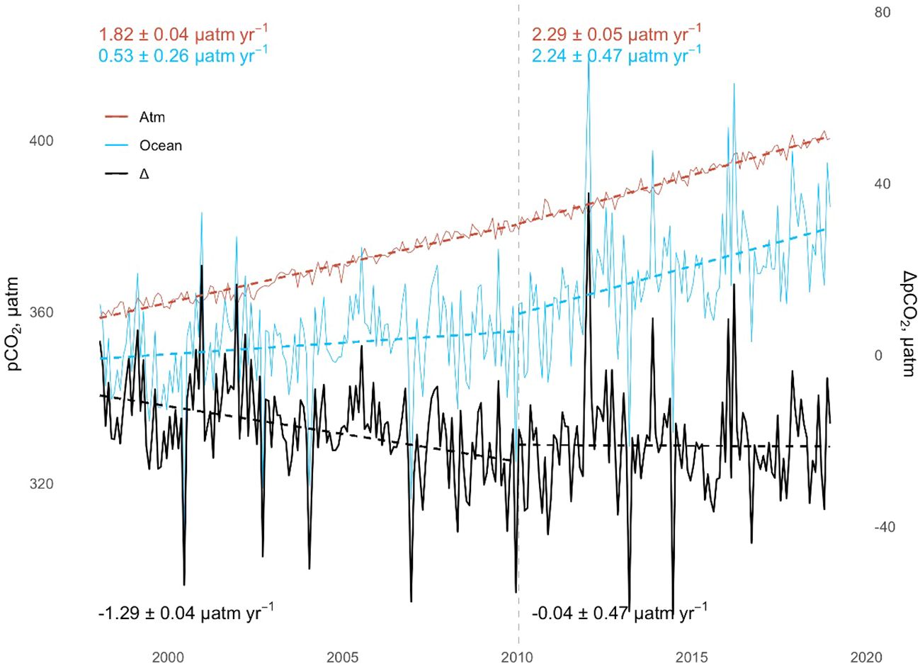
Figure 7 Time series of surface ocean pCO2 (blue), atmospheric pCO2 (red), and ΔpCO2 (black) with trends and associated uncertainties given for each decade showing a significant shift in 2010.
As the annual fluxes show no significant trends in net biological activity over this period (see Figure 6), this variability must be caused by changes in physical processes, or alternatively changes in biological productivity outside of the domain affecting advection of DIC through the region. To better understand the effects of decadal variability on the air-sea gas exchange, pCO2 was recalculated from the changes in temperature (thermal-corrected), changes in DIC from advection (advection-corrected), and also changes in DIC from horizontal mixing (mixing-corrected). Annual fluxes were then evaluated using these corrected pCO2 values following the detrending of the associated process with the inclusion of changes in solubility [K0(T,S)]. Figure 8 shows the effects of long-term trends in advection, temperature, solubility and mixing on the surface pCO2 gradient (9A) and the annual flux (8B). Note the mean seasonal cycle was removed from the temperature-corrected pCO2 values to show only the interannual and long-term variability. This indicates that warming accounted for an average reduction in surface CO2 flux of 40%, while changes in advection have increased the CO2 flux by 29%. Changes in mixing, assumed to be associated with variation in advection along the Southland Current and STF zone, had a smaller impact, reducing the CO2 flux by 8%. Changes in solubility imparted the smallest change, reducing the CO2 flux by 1%.
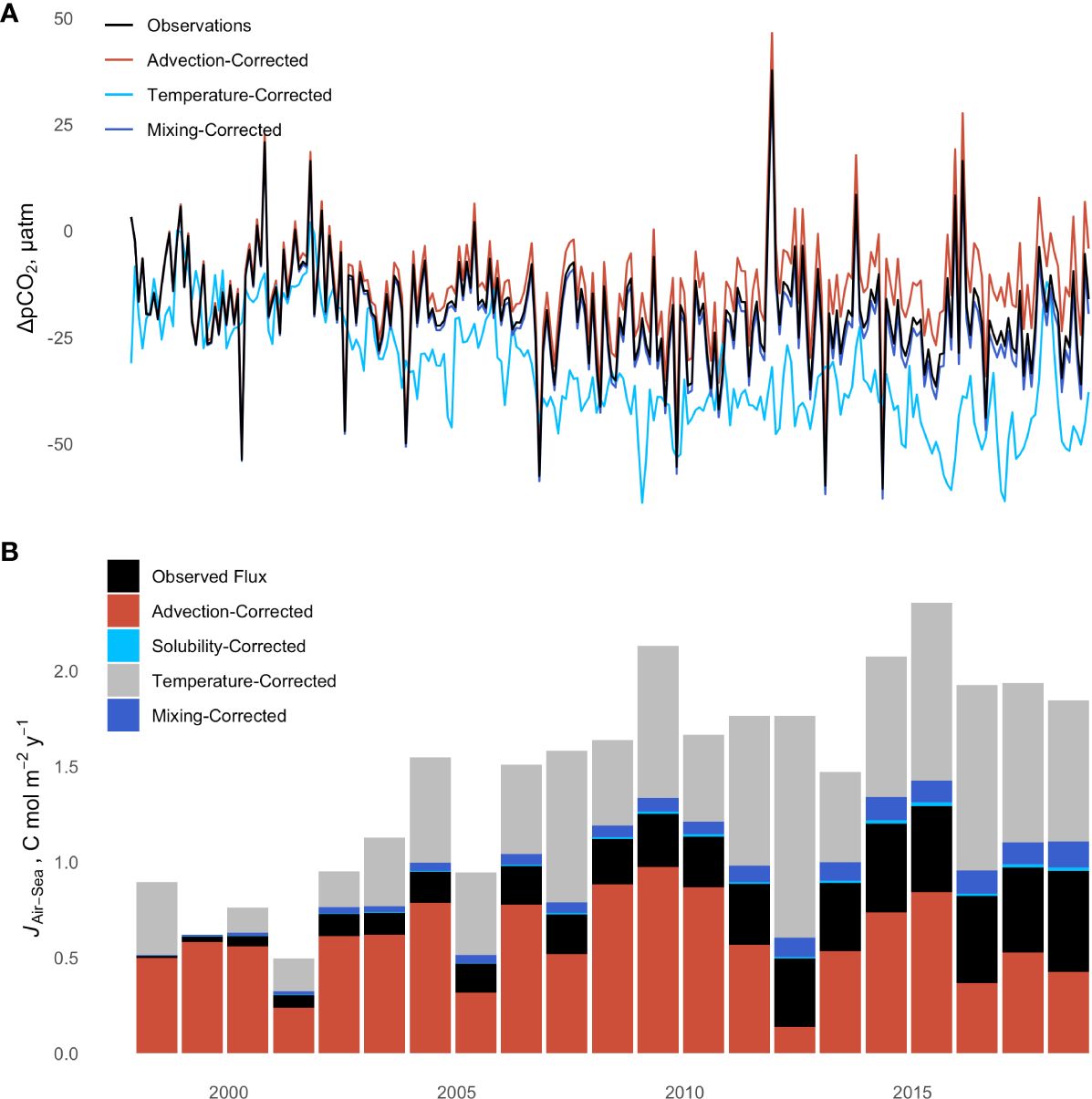
Figure 8 Timeseries of (A) the observed ΔpCO2 (black), with ΔpCO2 resulting from corrected advection (red), temperature (light blue), horizonal mixing (dark blue); and (B) annual fluxes of carbon due to the observed air-sea gas exchange (black) and the mean annual flux if there were no long-term changes in advection (red), solubility (light blue), temperature (grey) or horizontal mixing (dark blue).
The small changes in surface gradients of DIC suggest that weakening of the Southland Current is the primary driver of weaker advective fluxes (See Supplementary Figure S22). This is supported by the decadal trends of lower mean velocities in the mixed layer along the Southland Current (See Supplementary Figure S21). Regional evaluation of the heat and salinity budgets also indicated weakening advection along the Southland Current (Vance, 2023), which contributed to the thermal influence on pCO2 and surface fluxes.
Detrended cross correlation analysis (DCCA) quantifies the cross-correlation between nonstationary time series (Zebende, 2011), and was used here to assess the potential role of climate-scale variability on these estimated changes in surface layer carbon dynamics. DCCA was applied to the mixed layer temperature (MLT), salinity (MLS), DIC, DIC gradients (dCdx- zonal and dCdy - meridional), ΔpCO2, DIC advection term, and the velocity of the surface layer along the Southland Current (SC), to evaluate the cross-correlation with both the Southern Annular Mode (SAM) and Southern Oscillation Index (SOI). This approach provides cross-correlation over a range of frequencies. Here frequencies from 3 to 252 months were used to correspond to the duration of the MTS. Figure 9 shows the correlation coefficients between climate indexes and anomalies for each parameter after the seasonal cycle was removed. This analysis indicates some correlation in advection, DIC, SC, dCdx, dCdy, MLT and MLS in the 2- to 5-year frequency that is consistent with the ENSO-SOI time scale. Long-term changes in the Southland Current velocity appear to be strongly correlated with the SAM. Warming over the 20-year record, as shown in MLT, is partly correlated with the SAM while being anticorrelated with the SOI over that time scale. MLS is also anticorrelated with the SOI over this 20-year time scale. The DIC shows a correlation with the SOI, as does the advection term, while a correlation between SAM and advection is lacking over longer time scales suggesting long-term changes in surface gradients may contribute to changes in advection. However, when removing decadal variability from the gradients (dCdx and dCdy) the change in advection is not significant (See Supplementary Material Section 6).
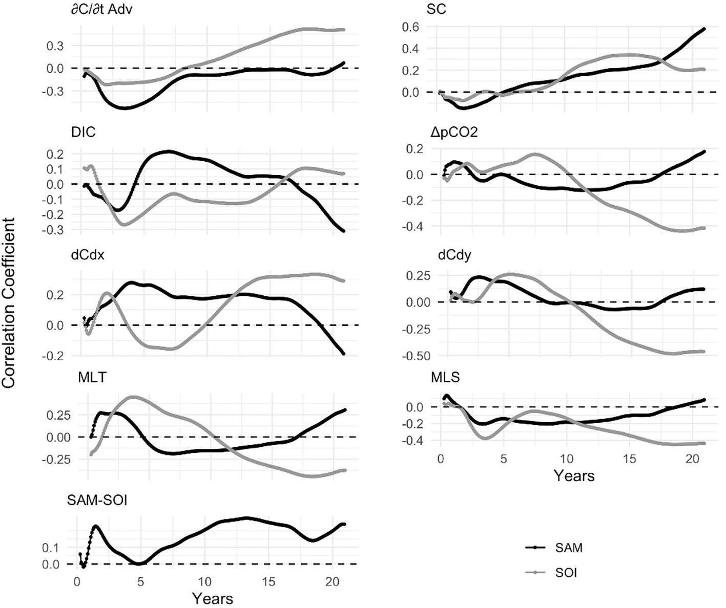
Figure 9 Detrended cross correlation coefficients between the advection of DIC, Southland Current velocity (SC), surface layer DIC concentration, ΔpCO2, zonal (dCdx) and meridional (dCdy) surface gradients in DIC, mixed layer temperature (MLT) and mixed layer salinity (MLS) and the Southern Annular Mode (SAM, black) and the Southern Oscillation Index (SOI, grey). Coefficients indicate the degree of correlation between time series at the given frequency (x-axes).
4 Discussion
The seasonal cycles presented in this study differ somewhat from previous estimates using a 13C-based diagnostic box model based upon 11 years of data collected in the MTS (Brix et al., 2013). The Brix (2013) evaluation indicated that NCP was the dominant DIC source term in the annual budget with diffusion and air-sea gas exchange contributing significantly, while horizontal advection and entrainment terms were less significant (less the 10% each). This updated analysis, incorporating an additional 9 years of data, confirms NCP as an important source term for the DIC budget, but conversely suggests that diffusion plays a smaller role in the annual budget. The mean annual NCP flux of 2.03 ± 3.10 mol C m-2 y-1 is greater than the 1.2 ± 0.7 mol C m-2 y-1 reported by Brix et al. (2013) but is consistent with the range of 1.2 ± 2.6 mol C m-2 y-1 reported by Jones (2012) for this region. These three estimates have large relative uncertainties, suggesting a high amount of variability, which is consistent with NCP being a dominant IAV term in the surface layer carbon cycle. The mean advective flux of 5.49 ± 1.02 mol C m-2 y-1 is greater than reported in that same study (Brix et al., 2013); however, dynamics were simulated in that study using a regional model that was poorly constrained with limited measurements outside of the Munida transect for estimating surface gradients. The mean air-sea gas exchange term presented here (0.84 ± 0.62 mol C m-2 y-1) is consistent with the 0.9 ± 0.1 mol C m-2 y-1 estimated over the period 1998 – 2010 (Brix et al. (2013). The difference in diffusion can be attributed to differences in the estimates of the vertical DIC gradient at the base of the mixed layer and the diffusivity parameterization. The MLR approaches used to estimate subpycnal DIC and TA concentrations lead to relatively larger uncertainty in the gradients at the base of the mixed layer affecting both the entrainment and diffusion estimates. Brix et al. (2013) did not parameterize horizontal mixing due to eddies, impacting the physical transport terms and thus the NCP estimates as well. Turbulence along the Southland Current likely drives mixing across the STF where zonal gradients between subtropical and subantarctic waters are steep, suggesting this is an important term to include in the carbon cycle evaluation (Vance, 2023). Additionally, the Brix model used a Heavyside function for entrainment that only allowed for the addition of DIC during deepening of the MLD (Gruber et al., 1998), whereas the detrainment term was used in this study, as in Cronin et al. (2015) and Yang et al. (2021).
The additional years of MTS observations and the availability of ancillary data also provided the opportunity to evaluate interannual to decadal-scale variability in the carbon cycle and impacts on regional acidification. However, during the seasonal integration to evaluate the dominant drivers of IAV there were several instances where the IAV was smaller than the uncertainty of mean annual contribution, making it difficult to attribute the process contribution to IAV. For each of the DIC, TA and pCO2 budgets this was the case for NCP, due to the large uncertainties associated with the residual following all other processes in the budget evaluation. This was also the case for calcification in the DIC and pCO2 budgets. Annual changes due to air-sea CO2 flux in the DIC budget and vertical entrainment in the pCO2 budget were of similar magnitude as their corresponding IAV. While the MLR approaches used for interpolation in this study have been shown to constrain IAV well, the uncertainties can become large when considering all sources, illustrating the limitation of this approach for deriving the contribution of individual processes to IAV in the carbon cycle. The significant long-term trends calculated for air-sea flux, advection, and horizontal mixing had uncertainties of 2%, 42%, and 30% respectively, providing greater confidence when considering their contributions to decadal variability in the carbon cycle relative to the other processes with higher uncertainty.
4.1 Regional acidification and carbon sink variability
This region remains a persistent sink for atmospheric CO2, which is increasing at a mean rate of 0.026 ± 0.006 mol C m-2 y-2. While long term increases in DIC and acidification are primarily driven by uptake of anthropogenic CO2 emissions, this budget evaluation indicates that advection contributed significantly to variability over seasonal to decadal time scales. The weakening advective flux of DIC in the region resulted in lower ocean pCO2, effectively maintaining the efficiency of the regional carbon sink. The mean ΔpCO2 over 2010 - 2019 was -21.2 μatm, which would have been reduced by over 42% to -12.2 μatm had there been no decline in DIC transport. An important conclusion of this is a mitigating effect on regional acidification. Detrending the advective flux component from the DIC and recalculating the pH indicates that the changes in regional ocean circulation have maintained the regional pH 0.011 ± 0.003 higher than it otherwise would have been due to atmospheric forcing alone.
This lowering of pCO2 by reduced advection was partly offset over the same time scale by increasing heat and salt content, which lowered CO2 solubility and resulted in higher pCO2 values, weakening ΔpCO2 and the air-sea flux. Decadal variability indicated K0(T,S) was weakly increasing during 1998–2010 then decreasing at a greater rate after 2010 (See Supplementary Figure S23). When accounting for the temperature change alone the pCO2 would have declined over 1998 – 2010 by 0.86± 0.2 μatm y-1 and then increased by 1.57 ± 0.3 μatm y-1 from 2010 – 2019. DIC increased significantly during 1998–2010 at a rate of 0.71 ± 0.15 μmol kg-1 y-1 (p< 3e-6) when temperatures were cooling, and solubility was increasing (See Supplementary Figure S23) but then slowed after 2010 to 0.26 ± 0.55 μmol kg-1 y-1 (p > 0.2) during a period of warming (0.1°C yr-1) concurrent with the declining advection. The changes in heat and density over these timescales are also apparent in the sea surface height anomalies for the region (See Supplementary Material), which is also reflected in the geostrophic flow, the primary component of the overall advective flux. Changes in advection of DIC are more consistent with changes in the geostrophic flow than variability in the horizontal gradients over these decades.
While seasonal and interannual variability is primarily controlled by advective fluxes and biological production, decadal variability appears to be largely affected by the regional heat budget, air-sea gas exchange and ocean circulation controlling DIC transport.
4.2 Regional dynamics and climate sensitivity
The dominant advection term in this regional carbon budget is primarily driven by the strong geostrophic transport of the Southland Current, which primarily delivers SAW (90% of flow) along the shelf break with a mean transport of 10 Sv +/- 1 Sv seasonally (Sutton, 2003; Fernandez et al., 2018). The DCCA shown in Figure 9 indicates a strong correlation between the Southland Current velocity and the SAM; however, the mechanism for this is not clear. Additionally, the correlation between advection and SAM is less apparent, particularly over longer time scales, while the correlation is stronger over these time scales to the SOI.
Fernandez et al. (2014) reported a positive trend in transport along the confluence of STW and SAW southeast of New Zealand with increasing eddy kinetic energy (EKE); this is consistent with more recent analyses of Argo floats, satellite altimeters, and model ensembles that identified accelerating flow along the SAF associated with spin-up and poleward shift of the South Pacific Subtropical Gyre (Shi et al., 2021). The thermally driven zonal acceleration observed in the ACC (and SAF) also indicates opposing trends just north of the SAF (Shi et al., 2021). One potential explanation for the weak downward trend in advection reported here is that the increased zonal flow of the ACC and increased EKE along the SAF, and Campbell Plateau in particular, may be weakening the deep water boundary current along the deep pathway of the SC formation. Additionally, the poleward migration of the EAC and its extension, as well as the associated increasing EKE west of the South Island, may be impacting the gradients in sea surface height and the shallow pathway of SC formation on the western margin of the Campbell Plateau (Li et al., 2022). However, further research is needed to better understand the drivers of SC variability.
The temperature and strength of the Southland Front, the subtropical front along the southeast shelf of New Zealand and SC, are correlated with ENSO, decreasing during El Nino and increasing during La Nina events (Hopkins et al., 2010). Hopkins et al. (2010) also indicate correlation between the strength of the SC and ENSO variability associated with the regional temperature gradients, which is consistent with the findings here. This would also support the positive correlation between DIC advection and SOI during la Nina episodes when advection is stronger. Conversely, the SOI is strongly negatively correlated to MLT, MLS and the surface pCO2, as shown by the DCCA (Section 3.3). While the SOI also shows a strong correlation with the DIC gradient, the changes in gradients over decadal time scales are less significant compared to changes in circulation when assessing the impact on advection.
Eastward flow of the ACC is interrupted by the submarine topographic features the Maquarie Ridge and the Campbell Plateau south of New Zealand, diverting the SAF northward (Morris et al., 2001). A Lagrangian modelling study showed that these and other topographic features in the Southern Ocean are important in delivering DIC-enriched waters from 1000 m depth to the surface through upwelling (Brady et al., 2021). Antarctic Intermediate Water (AAIW) originating from the SAF is present below 250 m beyond the shelf break at the MTS and has been shown to mix with surface water (Jillett, 1969; Chiswell et al., 2015). The Brady et al. (2021) study indicated AAIW contributes nearly 50% of upwelled DIC on the Campbell Plateau (versus 46% from Circumpolar Deep Water). These dynamics illustrate the connection of the southeastern shelf of New Zealand to the broader Southern Ocean and the pathway for advection of higher DIC into the region. However, while vertical entrainment contributed significantly to IAV there was no indication of long-term trends in that budget term. The entrainment flux term is also primarily driven by downwelling favorable winds across this region (Stevens et al., 2019).
The horizontal mixing term in this budget represents turbulent mixing, which is important along this strong frontal zone as indicated by its contribution to IAV, as well as a long-term increase in its contribution to the DIC concentration. Heat and salt budget analyses using a regional ocean model indicated that submesoscale eddies develop along the Southland Current and are an important feature driving mixing along the STF (Vance, 2023). Thus, here the horizontal mixing term represents the mixing of lower DIC and higher TA STW across the STF lowering the DIC in the SAW at the MTS station. The mixing term was typically negative prior to 2010, however concurrent with the weaker advection, warming temperatures, and weaker zonal gradients, this term shifts to a more neutral trend.
While the regional ocean pH continues to decline at a rate of approximately -0.016 pH units per decade due to the absorption of atmospheric CO2, it is not yet clear how that rate will evolve over future decades due to the complex processes controlling variability, as illustrated in this study. Current model projections indicate the Southern Ocean will continue to warm, driving changes in circulation and ventilation, and surface ocean pH around New Zealand may decline by as much as 0.3 by 2100 (Law et al., 2017; Negrete-García et al., 2019; Wang et al., 2022). New Zealand’s marginal seas are highly sensitive to changes in the South Pacific western boundary current system and Southern Ocean dynamics. Using estimates from biogeochemical profiling ARGO floats, Mazloff et al. (2023) showed that the upper 750m of the SAW, including the formation of SAMW, show some of the strongest acidification rates in excess of -0.02 pH units per decade due to being recently ventilated and equilibrated with high anthropogenic atmospheric CO2, further illustrating the higher relative sensitivity for this region to continued CO2 emissions.
This study underscores the value of maintaining the long-term Munida Time Series observations. These repeat measurements are required to understand natural variability and detect long-term trends, which are critical to developing strategies to address climate change. Such observational data are also critical for informing model development, to better understand the large-scale and complex interactions that control variability, such as those between the regional carbon cycle and climate indices as investigated here, and also to resolve decadal variability.
5 Conclusion
Twenty years of data from the Munida Time Series were used to evaluate the drivers of variability in the surface ocean carbon cycle over seasonal to decadal time scales. Observations of carbonate chemistry, meteorological conditions, and reanalysis of ocean physics were used to constrain the physical processes in a mass-balanced surface layer carbon budget to diagnostically assess the contributions from air-sea gas exchange, surface freshwater fluxes, physical transport processes, and biological productivity.
The results presented highlight that understanding future changes in the efficiency of the ocean sink for anthropogenic CO2 and associated acidification rates requires characterization of biogeochemical and physical processes across a range of scales. Developing the connection between regional and larger basin-scale ocean processes is critical to understanding drivers of spatiotemporal variability, sensitivity to climate change and enhancing the predictive power of models. While the MTS record is long enough for decadal patterns to emerge, it is not yet long enough to fully resolve decadal variability and further research is needed to better understand correlations between regional and climatological variability. Ongoing monitoring and additional observational sampling to better constrain ocean and Earth system model simulations will contribute to reducing uncertainty in future climate projections, aiding the development of targeted mitigation strategies to address climate change and ocean acidification.
Data availability statement
Gridded remotely sensed chlorophyll data produced by NASA is available from: https://coastwatch.pfeg.noaa.gov/erddap/griddap/index.html?page=1&itemsPerPage=1000. Global ocean Physical Reanalysis data produced by Copernicus Marine Services is available from: https://data.marine.copernicus.eu/product/GLOBAL_MULTIYEAR_PHY_001_030/description. Janapese 55-year Reanalysis data produced by the Japanese Meteorological Agency is available from: https://rda.ucar.edu/datasets/ds628.0/index.htmlajax/#cgi-bin/datasets/getSubset?dsnum=628.0&listAction=customize&_da=y&gindex=23. Atmospheric CO2 collected at Baring Head is included in the Observation Package (ObsPack) produced by the Global Monitory Laboratory within NOAA and is available here: https://gml.noaa.gov/ccgg/obspack/.
Author contributions
JV: Conceptualization, Data curation, Formal analysis, Investigation, Methodology, Software, Visualization, Writing – original draft, Writing – review & editing. KC: Conceptualization, Data curation, Funding acquisition, Project administration, Resources, Writing – review & editing. SS: Conceptualization, Writing – review & editing. CL: Writing – review & editing.
Funding
The author(s) declare financial support was received for the research, authorship, and/or publication of this article. This work was supported by the National Institute of Water and Atmospheric Research (NIWA) and the University of Otago. The research presented herein was supported financially by NIWA Research Scholarship Grant C 17959 to JV.
Acknowledgments
The authors thank Judith Murdoch for years of work in the field and lab in support of the Munida Time Series. We honor Keith Hunter a founding member of the New Zealand Ocean Acidification Community and was fundamental in establishing and maintain the collaboration between NIWA and the University of Otago and with KC, establishing and maintaining the Munida Time Series. This research is based in part on the data products produced by the US National Aeronautics and Space Administration (NASA), Copernicus Marine Services (CMEMS), the Japanese Meteorological Agency (JMA) and the Central Research Institute of Electric Power Industry (CRIEPI).
Conflict of interest
The authors declare that the research was conducted in the absence of any commercial or financial relationships that could be construed as a potential conflict of interest.
Publisher’s note
All claims expressed in this article are solely those of the authors and do not necessarily represent those of their affiliated organizations, or those of the publisher, the editors and the reviewers. Any product that may be evaluated in this article, or claim that may be made by its manufacturer, is not guaranteed or endorsed by the publisher.
Supplementary material
The Supplementary Material for this article can be found online at: https://www.frontiersin.org/articles/10.3389/fmars.2024.1309560/full#supplementary-material
References
Bailey S. W., Werdell P. J. (2006). A multi-sensor approach for the on-orbit validation of ocean color satellite data products. Remote Sens. Environ. 102 (1-2), 12–23. doi: 10.1016/j.rse.2006.01.015
Bates N., Astor Y., Church M., Currie K., Dore J., Gonaález-Dávila M., et al. (2014). A time-series view of changing ocean chemistry due to ocean uptake of anthropogenic CO2 and ocean acidification. Oceanography 27 (1), 126–141. doi: 10.5670/oceanog.2014.16
Bourgeois T., Orr J. C., Resplandy L., Terhaar J., Ethé C., Gehlen M., et al. (2016). Coastal-ocean uptake of anthropogenic carbon. Biogeosciences 13 (14), 4167–4185. doi: 10.5194/bg-13-4167-2016
Brady R. X., Maltrud M. E., Wolfram P. J., Drake H. F., Lovenduski N. S. (2021). The influence of ocean topography on the upwelling of carbon in the southern ocean. Geophys. Res. Lett. 48 (19), e2021GL095088. doi: 10.1029/2021GL095088
Brix H., Currie K. I., Mikaloff Fletcher S. E. (2013). Seasonal variability of the carbon cycle in subantarctic surface water in the South West Pacific. Global Biogeochem. Cycles 27 (1), 200–211. doi: 10.1002/gbc.20023
Carroll D., Menemenlis D., Dutkiewicz S., Lauderdale J. M., Adkins J. F., Bowman K. W., et al. (2022). Attribution of space-time variability in global-ocean dissolved inorganic carbon. Global Biogeochem. Cycles 36 (3), e2021GB007162. doi: 10.1029/2021GB007162
Chiswell S. M., Bostock H. C., Sutton P. J. H., Williams M. J. M. (2015). Physical oceanography of the deep seas around New Zealand: a review. New Z. J. Mar. Freshw. Res. 49 (2), 286–317. doi: 10.1080/00288330.2014.992918
Cox A., Di Sarra A. G., Vermeulen A., Manning A., Beyersdorf A., Zahn A., et al. (2021). Multi-laboratory compilation of atmospheric carbon dioxide data for the period 1957–2020.
Cronin M. F., Bond N. A., Thomas Farrar J., Ichikawa H., Jayne S. R., Kawai Y., et al. (2013). Formation and erosion of the seasonal thermocline in the Kuroshio Extension Recirculation Gyre. Deep Sea Res. Part II: Topical Stud. Oceanogr. 85, 62–74. doi: 10.1016/j.dsr2.2012.07.018
Cronin M. F., Pelland N. A., Emerson S. R., Crawford W. R. (2015). Estimating diffusivity from the mixed layer heat and salt balances in the North Pacific. J. Geophys. Res.: Oceans 120 (11), 7346–7362. doi: 10.1002/2015JC011010
Currie K. I., Macaskill B., Reid M. R., Law C. S. (2011a). Processes governing the carbon chemistry during the SAGE experiment. Deep Sea Res. Part II: Topical Stud. Oceanogr. 58 (6), 851–860. doi: 10.1016/j.dsr2.2010.10.023
Currie K. I., Reid M. R., Hunter K. A. (2011b). Interannual variability of carbon dioxide drawdown by subantarctic surface water near New Zealand. Biogeochemistry 104 (1-3), 23–34. doi: 10.1007/s10533-009-9355-3
de Souza J. M. A. C., Couto P., Soutelino R., Roughan M. (2020). Evaluation of four global ocean reanalysis products for New Zealand waters–A guide for regional ocean modelling. New Z. J. Mar. Freshw. Res. 55 (1), 132–155. doi: 10.1080/00288330.2020.1713179
DeVries T. (2022). Atmospheric CO2 and sea surface temperature variability cannot explain recent decadal variability of the ocean CO2 sink. Geophys. Res. Lett. 49 (7), 317–341. doi: 10.1029/2021GL096018
DeVries T., Holzer M., Primeau F. (2017). Recent increase in oceanic carbon uptake driven by weaker upper-ocean overturning. Nature 542 (7640), 215–218. doi: 10.1038/nature21068
Dickson A. G. (1979). The estimation of acid dissociation constants in seawater media from potentiometric titrations with strong base. Mar. Chem. 7, 101–109. doi: 10.1016/0304-4203(79)90002-1
Dickson A. G., Sabine C. L., Christian J. R. (2007). Guide to Best Practices for Ocean CO2 Measurements. Sidney, BC Canada.
Dickson A. G., Wesolowski D. J., Palmer D. A., Mesmer R. E. (1990). Dissociation constant of bisulfate ion in aqueous sodium chloride solutions to 250 oC. J. Phys. Chem. 94, 7978–7985. doi: 10.1021/j100383a042
Doney S. C., Fabry V. J., Feely R. A., Kleypas J. A. (2009). Ocean acidification: the other CO2Problem. Annu. Rev. Mar. Sci. 1, 169–192. doi: 10.1146/annurev.marine.010908.163834
Fassbender A. J., Sabine C. L., Cronin M. F. (2016). Net community production and calcification from 7 years of NOAA Station Papa Mooring measurements. Global Biogeochem. Cycles 30 (2), 250–267. doi: 10.1002/2015GB005205
Fassbender A. J., Sabine C. L., Cronin M. F., Sutton A. J. (2017). Mixed-layer carbon cycling at the Kuroshio Extension Observatory. Global Biogeochem. Cycles 31 (2), 272–288. doi: 10.1002/2016GB005547
Fernandez D., Bowen M., Carter L. (2014). Intensification and variability of the confluence of subtropical and subantarctic boundary currents east of New Zealand. J. Geophys. Res.: Oceans 119 (2), 1146–1160.
Fernandez D., Bowen M., Sutton P. (2018). Variability, coherence and forcing mechanisms in the New Zealand ocean boundary currents. Prog. Oceanogr. 165, 168–188. doi: 10.1016/j.pocean.2018.06.002
Friedlingstein P., Jones M. W., O'Sullivan M., Andrew R. M., Bakker D. C. E., Hauck J., et al. (2022). Global carbon budget 2021. Earth Sys. Sci. Data 14 (4), 1917–2005. doi: 10.5194/essd-14-1917-2022
Gattuso J.-P., Epitalon J.-M., Lavigne H., Orr J., Gentili B., Hagens M., et al. (2012) seacarb. Available online at: https://cran.r-project.org/web/packages/seacarb/seacarb.pdf.
Gregg M. C., D’Asaro E. A., Riley J. J. (2018). Mixing efficiency in the ocean. Annu. Rev. Mar. Sci. 10, 443–473. doi: 10.1146/annurev-marine-121916-063643
Gruber N., Kelling C. D., Stocker T. F. (1998). Carbon-13 constraints on the seasonal inorganic carbon budget at the BATS site in the northwestern Sargasso Sea. Deep Sea Res. 45, 673–717. doi: 10.1016/S0967-0637(97)00098-8
Hastie A., Lauerwald R., Weyhenmeyer G., Sobek S., Verpoorter C., Regnier P. (2018). CO2 evasion from boreal lakes: Revised estimate, drivers of spatial variability, and future projections. Glob. Chang. Biol. 24, 711–728. doi: 10.1111/gcb.13902
Ho D. T., Law C. S., Smith M. J., Schlosser P., Harvey M., Hill P. (2006). Measurements of air-sea gas exchange at high wind speeds in the Southern Ocean: Implications for global parameterizations. Geophys Res Lett. 33 (16).
Hopkins J., Shaw A. G. P., Challenor P. (2010). The Southland Front, New Zealand: variability and ENSO correlations. Continental Shelf Res. 30, 1535–1548. doi: 10.1016/j.csr.2010.05.016
Hurlburt H. E., Metzger E. J., Hogan P. J., Tilburg C. E., Shriver J. F. (2008). Steering of upper ocean currents and fronts by the topographically constrained abyssal circulation. Dynamics Atmos. Oceans 45, 102–134. doi: 10.1016/j.dynatmoce.2008.06.003
Imawaki S., Bower A. S., Beal L., Qiu B. (2013). “Western boundary currents,” in Ocean Circulation and Climate - A 21st Century Perspective (Oxford, UK: Elsevier), 305–338.
Jean-Michel L., Eric G., Romain B.-B., Gilles G., Angélique M., Marie D., et al. (2021). The Copernicus global 1/12° Oceanic and sea ice GLORYS12 reanalysis. Front. Earth Sci. 9. doi: 10.3389/feart.2021.698876
Jillett J. B. (1969). Seasonal hydrology of waters off the Otago peninsula, South-Eastern New Zealand. New Z. J. Mar. Freshw. Res. 3, 349–375. doi: 10.1080/00288330.1969.9515303
Johnson G. C., Lyman J. M. (2020). Warming trends increasingly dominate global ocean. Nat. Climate Change 10, 757–761. doi: 10.1038/s41558-020-0822-0
Jones K. N. B. (2012). Characterising the biological uptake of CO2 across the Subtropical Frontal Zone. University of Otago, Dunedin, New Zealand. (PhD).
Jones K. N., Currie K. I., McGraw C. M., Hunter K. A. (2013). The effect of coastal processes on phytoplankton biomass and primary production within the near-shore Subtropical Frontal Zone. Estuar. Coast. Shelf Sci. 124, 44–55. doi: 10.1016/j.ecss.2013.03.003
Keeling C. D., Brix H., Gruber N. (2004). Seasonal and long-term dynamics of the upper ocean carbon cycle at Station ALOHA near Hawaii. Global Biogeochem. Cycles 18, 2004GB002227. doi: 10.1029/2004GB002227
Kelly K. A., Small R. J., Samelson R. M., Qiu B., Joyce T. M., Kwon Y.-O., et al. (2010). Western boundary currents and frontal air–sea interaction: gulf stream and Kuroshio extension. J. Climate 23, 5644–5667. doi: 10.1175/2010JCLI3346.1
Kobayashi S., Ota Y., Harada Y., Ebita A., Moriya M., Onoda H., et al. (2015). The JRA-55 reanalysis: general specifications and basic characteristics. J. Meteorological Soc. Jpn. Ser. II 93, 5–48. doi: 10.2151/jmsj.2015-001
Lan X., Dlugokencky E. J., Mund J. W., Crotwell A. M., Crotwell M. J., Moglia E., et al. (2022). Atmospheric Carbon Dioxide Dry Air Mole Fractions from the NOAA GML Carbon Cycle Cooperative Global Air Sampling Network. New Zealand: Baring Head.
Law C. S., Bell J. J., Bostock H. C., Cornwall C. E., Cummings V. J., Currie K., et al. (2018). Ocean acidification in New Zealand waters: trends and impacts. New Z. J. Mar. Freshw. Res. 52, 155–195. doi: 10.1080/00288330.2017.1374983
Law C. S., Rickard G. J., Mikaloff-Fletcher S. E., Pinkerton M. H., Behrens E., Chiswell S. M., et al. (2017). Climate change projections for the surface ocean around New Zealand. New Z. J. Mar. Freshw. Res. 52, 309–335. doi: 10.1080/00288330.2017.1390772
Lellouche J.-M., Legalloudec O., Regnier C., Van Gennip S., Law Chune S., Levier B., et al. (2023a). Quality Information Document: Global Sea Physical Analysis and ForecastingProduct GLOBAL_ANALYSISFORECAST_PHY_001_024.
Lellouche J.-M., Le Galloudec O., Regnier C., Van Gennip S., Law Chune S., Levier B., et al. (2023b). Quality Information Document for Global Sea Physical Analysis and Forecasting Product GLOBAL_ANALYSISFORECAST_PHY_001_024 (CMEMS-GLO-QUID-001–024).
Li J., Roughan M., Kerry C. (2022). Drivers of ocean warming in the western boundary currents of the Southern Hemisphere. Nat. Climate Change 12, 901–909. doi: 10.1038/s41558-022-01473-8
Lueker T. J., Dickson A. G., Keeling C. D. (2000). Ocean pCO2 calculated from dissolved inorganic carbon, alkalinity, and equations for K1 and K2: validation based on laboratory measurements of CO2 in gas and seawater at equilibrium. Mar. Chem. 70, 105–110. doi: 10.1016/S0304-4203(00)00022-0
Mazloff M. R., Verdy A., Gille S. T., Johnson K. S., Cornuelle B. D., Sarmiento J. (2023). Southern ocean acidification revealed by biogeochemical-argo floats. J. Geophys. Res.: Oceans 128, e2022JC019530. doi: 10.1029/2022JC019530
Morley S. A., Abele D., Barnes D. K. A., Cárdenas C. A., Cotté C., Gutt J., et al. (2020). Global drivers on southern ocean ecosystems: changing physical environments and anthropogenic pressures in an earth system. Front. Mar. Sci. 7. doi: 10.3389/fmars.2020.547188
Morris M., Stanton B., Neil H. (2001). Subantarctic oceanography around New Zealand: Preliminary results from an ongoing survey. New Z. J. Mar. Freshw. Res. 35, 499–519. doi: 10.1080/00288330.2001.9517018
Negrete-García G., Lovenduski N. S., Hauri C., Krumhardt K. M., Lauvset S. K. (2019). Sudden emergence of a shallow aragonite saturation horizon in the Southern Ocean. Nat. Climate Change 9, 313–317. doi: 10.1038/s41558-019-0418-8
Odon P., West G., Stull R. (2019). Evaluation of reanalyses over British Columbia. Part II: daily and extreme precipitation. J. Appl. Meteorol. Climatol. 58, 291–315. doi: 10.1175/JAMC-D-18-0188.1
Okubo A. (1971). Oceanic diffusion diagrams. Deep Sea Res. 18, 789–802. doi: 10.1016/0011-7471(71)90046-5
Onogi K., Tsutsui J., Koide H., Sakamoto M., Kobayashi S., Hatsuchika H., et al. (2007). The JRA-25 reanalysis. J. Meteorological Soc. Jpn. 85, 369–432. doi: 10.2151/jmsj.85.369
O’Reilly J. E., Maritorena S., Mitchell B. G., Siegel D. A., Carder K. L., Garver S. A., et al. (1998). Ocean color chlorophyll algorithms for SeaWiFS. J. Geophys. Res. 103, 24,937–924,953.
Orr J. C., Epitalon J.-M., Dickson A. G., Gattuso J.-P. (2018). Routine uncertainty propagation for the marine carbon dioxide system. Mar. Chem. 207, 84–107. doi: 10.1016/j.marchem.2018.10.006
Randerson J. T., Lindsay K., Munoz E., Fu W., Moore J. K., Hoffman F. M., et al. (2015). Multicentury changes in ocean and land contributions to the climate-carbon feedback. Global Biogeochem. Cycles 29, 744–759. doi: 10.1002/2014GB005079
R Core Team. (2020). R: A Language and environment for statistical computing. Retrieved from https://www.R-project.org/.
Safi K. A., Rodríguez A. G., Hall J. A., Pinkerton M. H. (2023). Phytoplankton dynamics, growth and microzooplankton grazing across the subtropical frontal zone, east of New Zealand. Deep Sea Res. Part II: Topical Stud. Oceanogr. 208, 105271. doi: 10.1016/j.dsr2.2023.105271
Sarmiento J. L., Gruber N. (2006). Ocean Biogeochemical Dynamics (Princeton, NJ, USA: Princeton University Press).
Schellnhuber H. J., Rahmstorf S., Winkelmann R. (2016). Why the right climate target was agreed in Paris. Nat. Climate Change 6, 649–653. doi: 10.1038/nclimate3013
Shi J.-R., Talley L. D., Xie S.-P., Peng Q., Liu W. (2021). Ocean warming and accelerating Southern Ocean zonal flow. Nat. Climate Change 11, 1090–1097. doi: 10.1038/s41558-021-01212-5
Stevens C. L., O’Callaghan J. M., Chiswell S. M., Hadfield M. G. (2019). Physical oceanography of New Zealand/Aotearoa shelf seas – a review. New Z. J. Mar. Freshw. Res. 55, 1–40. doi: 10.1080/00288330.2019.1588746
Stoddard I., Anderson K., Capstick S., Carton W., Depledge J., Facer K., et al. (2021). Three decades of climate mitigation: why haven't we bent the global emissions curve? Annu. Rev. Environ. Resour. 46, 653–689. doi: 10.1146/annurev-environ-012220-011104
Sutton P. J. H. (2003). The Southland Current: A subantarctic current. New Z. J. Mar. Freshw. Res. 37, 645–652. doi: 10.1080/00288330.2003.9517195
Thoning K. W., Tans P., Komhyr W. D. (1989). Atmospheric carbon dioxide at Mauna Loa observaotry 2. Analysis of the NOAA GMCC data 1974–1985. J. Geophys. Res. 94, 8549–8565. doi: 10.1029/JD094iD06p08549
Tilburg C. E., Hurlburt H. E., O'Brien J. J., Shriver J. F. (2002). Remote topographic forcing of a baroclinic western boundary current: an explanation for the southland current and the pathway of the subtropical front east of New Zealand. J. Phys. Oceanogr. 32, 3216–3232. doi: 10.1175/1520-0485(2002)032<3216:RTFOAB>2.0.CO;2
Vance J. (2023). Evaluating The Drivers Of Air-Sea Co2 Exchange And Ocean Acidification In Coastal Waters Around New Zealand. Otago University, Dunedin, New Zealand. (Doctor of Philosophy (Oceanography) Dissertation).
Vance J. M., Currie K., Zeldis J., Dillingham P. W., Law C. S. (2022). An empirical MLR for estimating surface layer DIC and a comparative assessment to other gap-filling techniques for ocean carbon time series. Biogeosciences 19, 241–269. doi: 10.5194/bg-19-241-2022
Vijith V., Vinayachandran P. N., Webber B. G. M., Matthews A. J., George J. V., Kannaujia V. K., et al. (2020). Closing the sea surface mixed layer temperature budget from in situ observations alone: Operation Advection during BoBBLE. Sci. Rep. 10, 7062. doi: 10.1038/s41598-020-63320-0
Wang G., Cai W., Santoso A., Wu L., Fyfe J. C., Yeh S.-W., et al. (2022). Future Southern Ocean warming linked to projected ENSO variability. Nat. Climate Change 12, 649–654. doi: 10.1038/s41558-022-01398-2
Weiss R. F. (1974). Carbon dioxide in water and seawater: the solubility of a non-ideal gas. Mar. Chem. 2, 203–215. doi: 10.1016/0304-4203(74)90015-2
Wen C., Kumar A., Xue Y. (2018). Uncertainties in reanalysis surface wind stress and their relationship with observing systems. Climate Dynamics 52, 3061–3078. doi: 10.1007/s00382-018-4310-4
White I. R., Royston P., Wood A. M. (2011). Multiple imputation using chained equations: Issues and guidance for practice. Stat. Med. 30, 377–399. doi: 10.1002/sim.4067
Williams N. L., Juranek L. W., Feely R. A., Russell J. L., Johnson K. S., Hales B. (2018). Assessment of the carbonate chemistry seasonal cycles in the southern ocean from persistent observational platforms. J. Geophys. Res.: Oceans 123, 4833–4852. doi: 10.1029/2017JC012917
Yang B., Shadwick E. H., Schultz C., Doney S. C. (2021). Annual mixed layer carbon budget for the West Antarctic Peninsula continental shelf: insights from year-round mooring measurements. J. Geophys. Res.: Oceans 126, e2020JC016920. doi: 10.1029/2020JC016920
Keywords: Carbon cycle, ocean acidification, Southern Ocean, variability, air-sea CO2 flux, surface layer budget, New Zealand, regional circulation
Citation: Vance JM, Currie K, Suanda SH and Law CS (2024) Drivers of seasonal to decadal mixed layer carbon cycle variability in subantarctic water in the Munida Time Series. Front. Mar. Sci. 11:1309560. doi: 10.3389/fmars.2024.1309560
Received: 08 October 2023; Accepted: 20 May 2024;
Published: 04 July 2024.
Edited by:
Xianghui Guo, Xiamen University, ChinaReviewed by:
Leticia Cotrim Da Cunha, Rio de Janeiro State University, BrazilPaula C. Pardo, Spanish National Research Council (CSIC), Spain
Copyright © 2024 Vance, Currie, Suanda and Law. This is an open-access article distributed under the terms of the Creative Commons Attribution License (CC BY). The use, distribution or reproduction in other forums is permitted, provided the original author(s) and the copyright owner(s) are credited and that the original publication in this journal is cited, in accordance with accepted academic practice. No use, distribution or reproduction is permitted which does not comply with these terms.
*Correspondence: Jesse M. Vance, jesse.vance@icloud.com