Scale-to-scale energy flux in the oceanic global circulation models

Lewis Fry Richardson proposed his famous picture of turbulent flows in 1922, where the kinetic energy is transferred from large-scale to small-scale structures until the viscosity converts it into heat. This cascade idea, also known as the forward energy cascade, is now widely accepted and is treated as the cornerstone of not only turbulent modeling, but also global circulation models of the ocean and atmosphere. In this work, the Filter-Space-Technique is applied to the oceanic flow field provided by the CMEMS reanalysis model to quantify the scale-to-scale energy flux. A rich dynamical pattern associated with different scales is observed. More precisely, either positive or negative fluxes are observed, indicating the direction of the energy cascade, where the energy is transferred from large-scale structures to small-scale ones or vice versa. High-intensity energy exchange is found mainly in the Western Boundary Current Systems and Equatorial Counter Currents. For the latter case, a wavelike pattern is observed on the westward travel. Moreover, strong seasonal variation is evident for some scales and regions. These results confirm the existence of forward and inverse cascades and rich regional dynamics.

1 Introduction

Turbulence phenomena are relevant in atmospheric and oceanic motions from both small-scale fluctuations (Frisch, 1995) and large-scale circulation (Nastrom et al., 1984; Thorpe, 2005). In 1922, in the book Weather Prediction by Numerical Process, Lewis Fry Richardson proposed his famous cascade picture to describe turbulent flows qualitatively (Richardson, 1922, p66), Big whirls have little whirls that feed on their velocity, and little whirls have lesser whirls and so on to viscosity–in the molecule sense. This concept is now considered as a cornerstone of both turbulent theory, e.g., Kolmogorov’s 1941 three-dimensional (3D) homogeneous and isotropic theory of turbulence (Kolmogorov, 1941b), Kraichnan’s theory of two-dimensional (2D) turbulence (Kraichnan, 1967), Charney’s geostrophic turbulence (Charney, 1971) etc., to name a few, and modeling, e.g., turbulent models (Chou, 1940, 1945; Landau and Lifshits, 1987; Pope, 2000; Davidson, 2004), global circulation model of the atmosphere and oceans (Thorpe, 2005; Vallis, 2017; Lovejoy, 2019). To have a quantitative characterization of the cascade, a proper diagnosis method is required (Alexakis and Biferale, 2018). For instance, the famous four-fifth law derived from the Navier-Stokes equation (NSE) has been proposed for third-order longitudinal structure-function in the so-called inertial range of the 3D homogeneous and isotropic turbulence (Kolmogorov, 1941a), which is written as

$\begin{array}{ll}{\langle (u_{\overrightarrow{\mathbf{\text{r}}}}(\overrightarrow{\mathbf{\text{x}}}+\overrightarrow{\mathbf{\text{r}}})-u_{\overrightarrow{\mathbf{\text{r}}}}(\overrightarrow{\mathbf{\text{x}}}))}^3\rangle =-\frac{4}{5}\overline{ϵ}r,& (1)\end{array}$

where 〈·〉 means ensemble average, and $u_{\overrightarrow{\mathbf{\text{r}}}}$ is the velocity component along the vector $\overline{\mathbf{\text{r}}}$, and $\overline{ϵ}$ is the mean energy dissipation rate per unit mass. This relation has been treated as one of the most important results of the Kolmogorov’s 1941 theory that has been verified both experimentally and numerically (Frisch, 1995). However, the interpretation of its generalization to other types of flows should be done with caution since the external forcing and dissipation balance are unknown; see a detailed discussion by Alexakis and Biferale (2018) and Zhou (2021).

Another possible flux estimator is based on the NSE in the spectral domain. Note that the temporal evolution of the kinetic energy spectrum E(k) can be derived from the NSE in the spectral domain as,

$\begin{array}{ll}\frac{\partial E(k)}{\partial t}=T(k)-2\upsilon \text{Ω}(k),& (2)\end{array}$

where T(k) represents the rate of energy transfer at the wavenumber k (i.e., k = 1/r) owing to nonlinear interactions (Kraichnan and Montgomery, 1980); υ is the fluid viscosity; Ω(k) = k²E(k) is the enstrophy spectrum. Note that this relation is only suitable for two-dimensional and quasi-geostrophic turbulence. The energy flux of the velocity field in the Fourier space is written as (Alexakis and Biferale, 2018; Zhou, 2021),

$\begin{array}{ll}\Pi (k)={\displaystyle {\int }_k^{\infty }T(k^{\prime })}d{k}^{\prime }.& (3)\end{array}$

In the turbulence research community, this approach (i.e., Equation (3)) has been widely used to estimate scale-to-scale energy fluxes since the domains of numerical simulation and laboratory experiments are regular (Scott and Wang, 2005; Scott and Arbic, 2007; Bai et al., 2013; Khatri et al., 2018). Note that this Fourier-based method is a global representation of the energy flux, where the homogeneous assumption is employed implicitly. The motion of oceanic flow is often inhomogeneous with complex boundaries, and thus this approach is not suitable for such problems. Nevertheless, the spectral approach could also be applied to ocean modeling dataset. For example, Sérazin et al. (2018) studied the inverse kinetic energy cascade with ocean general circulation models in the spectral domain, and they argued that the inverse kinetic energy cascade is a source of intrinsic variability of the ocean.

An alternative choice to estimate the cross-scale flux is the Filter-Space-Technique (FST, see definition in section 2), also known as the coarse-graining approach. It was introduced in the field of turbulence for Large Eddy Simulation (LES), where large-scale motions of a turbulent flow are resolved numerically, while unresolved small-scale ones are expressed using a turbulence model (Leonard, 1975; Pope, 2000). The key information is the physical quantity, such as energy, enstrophy, and other scalars (e.g., temperature, salinity, etc.), to mention a few, transferred between resolved and unresolved motions, which can be calculated a posteriori to quantify the local cascade in the physical domain (Eyink, 2005). Since it preserves local information, the homogeneous assumption here is unnecessary.

In recent years, FST and the associated “coarse-graining” approach have attracted more and more attention not only in fluid dynamics (Chen et al., 2006; Aluie and Kurien, 2011; Ni et al., 2014; Rivera et al., 2014; Fang and Ouellette, 2016; Zhou et al., 2016; Wang and Huang, 2017; Dong et al., 2020), but also in geophysical fields (Aluie et al., 2018; Barkan et al., 2021; Buzzicotti1 et al., 2021; Grooms et al., 2021; Rai et al., 2021; De Leo and Stocchino, 2022; Garabato et al., 2022; Steinberg et al., 2022; Contreras et al., 2023; Loose et al., 2023; Srinivasan et al., 2023). For example, Ni et al. (2014) showed that the FST is quite robust for different spatial resolutions. Wang and Huang (2017) confirmed the existence of the inverse energy cascade by applying the FST method to the experimental 2D bacterial turbulence velocity field. By applying the FST approach to data from a high-resolution eddy primitive equation model of the North Atlantic Ocean, Aluie et al. (2018) found forward and inverse (i.e., backward) cascades of energy fluxes. Barkan et al. (2021) showed that the decrease in the mesoscale kinetic energy is associated with an internal wave-induced reduction of the inverse energy cascade and an enhancement of the forward energy cascade from sub- to super-inertial frequencies. Garabato et al. (2022) further verified the seasonal variation of the energy transferred between the mesoscale and submesoscale motions in the open ocean. Sun et al. (2023) applied the “coarse-graining” approach to separate the gravity wave with three different types of filter kernel. Their results show that the final results might depend on the choice of kernels (e.g., Gaussian, top-hat and sharp spectral) (Beck and Kurz, 2021).

In this work, a Fast-Fourier-Transform based convolution was used to accelerate the computation of the FST, where the missing data (e.g., complex boundary, island, etc.), was overcome by introducing a mask matrix. It was then applied to a global reanalysis dataset to retrieve the global scale-to-scale energy flux. Section 2 presents the data and method; and results are given in section 3. Finally, the conclusion and discussion are presented in section 4.

2 Data and method

2.1 CMEMS reanalysis data

The CMEMS (Copernicus Marine Environment Monitoring Service) database used in this study is the GLORYS12V1 (Global Ocean Physics Reanalysis) reanalysis product of the global ocean eddy-permitting (1/12 degree horizontal resolution, approximately 8km, and 50 vertical levels) (Hewitt et al., 2020) that covers the altimetry since 1993 to 2023, which is available at https://resources.marine.copernicus.eu with a spatial extent from 80°S to 90°N. It is based largely on the real-time global forecasting CMEMS system, where the NEMO (Nucleus for European Modelling of the Ocean) platform is driven at the surface by ECMWF (European Centre for Medium-Range Weather Forecasts) ERA-Interim reanalysis. All available observations are assimilated by reduced-order Kalman filtering. Moreover, a 3D-VAR (three-dimensional variational data assimilation) scheme provides a correction for the slowly evolving large-scale biases in temperature and salinity. This resolution level, although too coarse to resolve the submesoscale and 3D turbulence, can be used for the mesoscale turbulence dynamics (Chassignet and Xu, 2017; Uchida et al., 2019). In this work, only the velocity field at the ocean surface (i.e., 0.49 m below the surface) is considered on the period from 1 January 1993 to 31 March 2023. This choice is partially due to the fact that the ocean surface is in the marine-atmosphere boundary layer, where strong air-sea interactions are found. Note that there are 2041 grid points in the meridional direction and 4320 grid points in the zonal direction; the correction as discussed in Refs (Aluie, 2019; Storer et al., 2022). from the geographic coordinate system to the Cartesian coordinate system is considered.

2.2 Filter-Space-Technique

Taking a two dimensional velocity field, e.g., u(x, t) = [u_x(x, y, t), u_y(x, y, t)] as an example, its lower-pass coarse-graining field is defined as (Aluie et al., 2018),

$\begin{array}{ll}{\mathbf{\text{u}}}^{(r)}(\mathbf{\text{x}}, t)=\mathbf{\text{u}}(\mathbf{\text{x}}, t)\ast G_r(\mathbf{\text{x}},t)={\displaystyle {\int }_{\left|{\text{x}}^{\prime }\right|\le r}\mathbf{\text{u}}}(\mathbf{\text{x}}+{\mathbf{\text{x}}}^{\prime },t)G_r({\mathbf{\text{x}}}^{\prime }, t)d{\mathbf{\text{x}}}^{\prime },& (4)\end{array}$

where ∗ is the convolution, G_r(x) is a filter kernel, and r is the spatial scale. Partially due to the fact that the Gaussian kernel, i.e., G_r(x) ∝ exp(−|x|²/2r²), has good low-pass properties in the Fourier space, it is often taken as the filter kernel (Boffetta and Ecke, 2012). Note that other types of kernel could also be applied in the Equation (4). As discussed by Aluie et al. (2018), for different choice of kernels the analysis result could be modified quantitatively, but not qualitatively. The scale-to-scale energy flux can be derived from the incompressible NSE, which is written as (Aluie et al., 2018; Dong et al., 2020),

$\begin{array}{ll}{\Pi }^{(r)}(\mathbf{\text{x}},t)=-{\displaystyle \sum _{i,j=1,2}\left[{(u_i{u}_j)}^{(r)}-\left(u_i{}^{(r)}{u}_j{}^{(r)}\right)\right]}\frac{\partial u_i^{(r)}}{\partial x_j},& (5)\end{array}$

where u₁ = u_x, u₂ = u_y are the velocity component, x₁ = x, x₂ = y are the spatial coordinates in the horizontal plane. A positive Π^(r) > 0 indicates that the energy is transferred from large-scale motions with spatial scale ℓ ≥ r to small-scale ones ℓ ≤ r, and vice versa. It thus characterizes both the direction and intensity of the energy cascade. Note that only the nonlinear term in the NSE is involved in the interscale interaction. The diagnosis of the redistribution of energy associated with different scales in space could also be performed using this coarse-graining method.

Note that in reconciling the coordinate problem from the spheric to the Cartesian one, the transformation is performed as discussed by Aluie (2019). In practice, the zonal and meridional velocities (u, v) are first projected on the Cartesian coordinates to obtain ( $u_x,u_y,u_z$) through the Equation (6) as follows,

$\begin{array}{ll}\begin{array}{l}{u}_x=-u\sin (\lambda )-v\text{cos}(\lambda )\text{sin}(\psi )\\ u_y=u\cos (\lambda )-v\text{sin}(\lambda )\text{sin}(\psi )\\ u_z=v\cos (\psi )\end{array}& (6)\end{array}$

where λ and ψ are longitude and latitude. The “coarse-grained” version $(u_x^{(r)},u_y^{(r)},u_z^{(r)})$ are then calculated on the surface of the sphere with a Gaussian kernel G_r(x). The final scale-to-scale flux is then estimated by Equation (5). In this work, to have a reasonable computational time, Π^(r) is estimated on the range 70°S to 70°N, and the kernel G_r(x) is updated with a step of 1° along the latitude to keep the same area of the kernel for all latitude, without any special treatments for the boundary.

The main shortcoming of the FST method is its heavy computational cost since the convolution operator is involved to perform the low-pass field; and the diagnosis results occupy a lot of storage space, since for each scale one needs the same size of storage as the raw field. In practice, the convolution is done using the Fast Fourier-Transform (FFT) based algorithm, thus the computational cost is acceptable even for the 3D case (Dong et al., 2020).

2.3 Missing data and complex boundary

As mentioned above, in practice, it is inevitable that the analyzed data possess either irregular domains with complex boundaries or missing data. To overcome this problem, the following algorithm is proposed for the 2D case to improve the FST method:

1) generate a regular data set in a 2D domain by replacing missing data or irregular parts with zeros;

2) generate a mask matrix to label the valid data;

3) perform the FFT-based convolution operation to both the regular data and the mask matrix, and calculate the scale-to-scale flux;

4) choose the valid local scale-to-scale flux via a mask matrix-based threshold.

Note that the spatial convolution can be done directly in the physical domain without involving steps 1) and 2), but with more heavy computation. For example, the computational complexity of the FFT-based convolution is roughly 𝒪(3M N ln M ln N) (the zero-padding is not taken into account) and is independent of the scale r, while that of the direct convolution is 𝒪(M N r²), where M and N are the dimensions of the domain analyzed in points, and r is the scale in points (Press et al., 1992). The ratio of computational complexity between FFT-based and direct convolution can be roughly estimated as 3lnM ln N/r². Taking a value of M = N = 1000 and r = 100 (in data points), this ratio is around 0.014. A numeric test shows a relative error of less than 2% for the mean energy flux ${\tilde{\Pi }}^{(r)}$ if a threshold 95% is chosen for the mask matrix; see a detailed test of this methodology in Gao (2022). Therefore, this threshold value is used in this study.

3 Results

In this work, the energy flux Π^(r) is calculated using the aforementioned algorithm for the daily mean surface velocity field with spatial scales from 50km to 1000km (e.g., from 6 to 125 grid points in the equatorial area), for example, from mesoscale eddies to oceanic circulation. Seasonal variations of global patterns are presented. The energy flux in several areas of interest, for instance, the Kuroshio Current or the Equatorial Counter Current (ECC), is then examined in detail.

3.1 Global pattern

Figure 1 shows the seasonal average Π^(r) for scales from r ≃ 50km to r ≃ 1000km, in which the first baroclinic Rossby radius of deformation (Chelton et al., 1998), which is defined outside of the equatorial band as $r_R\simeq \frac{1}{2\text{Ω}\left|\sin (\psi )\right|\pi }{\displaystyle {\int }_{-H}^{0}N(z)dz} (\text{Ω}$ is the rotation rate of the Earth, ψ is the latitude, H is the water depth and N²(z) is the squared buoyancy frequency), is illustrated as a contour line. For all scales, a rich dynamical pattern is observed. For example, a relatively high intensity of Π^(r) is observed in the Western Boundary Current (WBC). For example, for the case r ≃ 50km, a strong negative value of Π^(r) is observed in several WBC systems, such as the Gulf Stream, Kuroshio Current, Agulhas Current, Brazil Current, etc., to name a few. Note that in these areas (where the latitude is above 10°), the Rossby radius of deformation is roughly in the range 30 ≲ r_R≲ 100km, which can be treated as the typical spatial size of mesoscale eddies. The pattern of strong negative Π^(r) suggests an inverse energy cascade that transfers energy from structures with r ≲ 50 km to those with r ≳ 50km, which might be associated with the so-called “graveyard of the mesoscale eddies” (Zhai et al., 2010; Yang et al., 2021; Evans et al., 2022). With the increase of the scale r, the measured Π^(r) gradually increases to a positive value, indicating the changing from the inverse energy cascade to the forward one; see also Figure 2 for a longitude averaged energy fluxes ${\tilde{\Pi }}^{(r)}$ for four seasons. One should pay more attention to the ECC area, since there is absence of the Coriolis force, thus showing a quite different evolution trend compared other regions. The measured Π^(r) seems to be opposite to the one in the WBC area: it decreases with increasing scale r, which might be the effect of the equatorial jet, since the cascade depends strongly on the type of external forcing (Alexakis and Biferale, 2018). The asymmetric pattern is observed for all scales considered here. For example, for the case r = 50km and r = 100km a stronger positive Π^(r) is observed in the North ECC (e.g., 0°N to 10°N and 180°W to 80°W) than those observed in the South ECC (e.g., 10°S to 0°S and 180°W to 80°W). For larger scales r, the measured Π^(r) is strongly negative, implying an upscale energy transfer to the oceanic circulation, which has been observed in the laboratory (Xia et al., 2011). A seasonal variation is observed: For instance, a strong positive Π^(r) intrusion is observed for the case r = 1000km in JJA and SON; see Figure 1D. One possible reason for this asymmetric pattern and intrusion is the effect of land coverage. The global map of the measured Π^(r) thus indicates a strong variation of the dynamics not only in space but also in time.

Figure 1

Figure 1 Seasonal average energy flux Π^(r) on typical scales from r ≃ 50km to r ≃ 1000km. The contour line indicates the Rossby radius of deformation r_R provided in Chelton et al. (1998). (A) Seasonal average of Π^(r) for spatial scale r ≃ 50km. (B) Seasonal average of Π^(r) for spatial scale r ≃ 100km. (C) Seasonal average of Π^(r) for spatial scale r ≃ 500km. (D) Seasonal average of Π^(r) for spatial scale r ≃ 1000km.

Figure 2

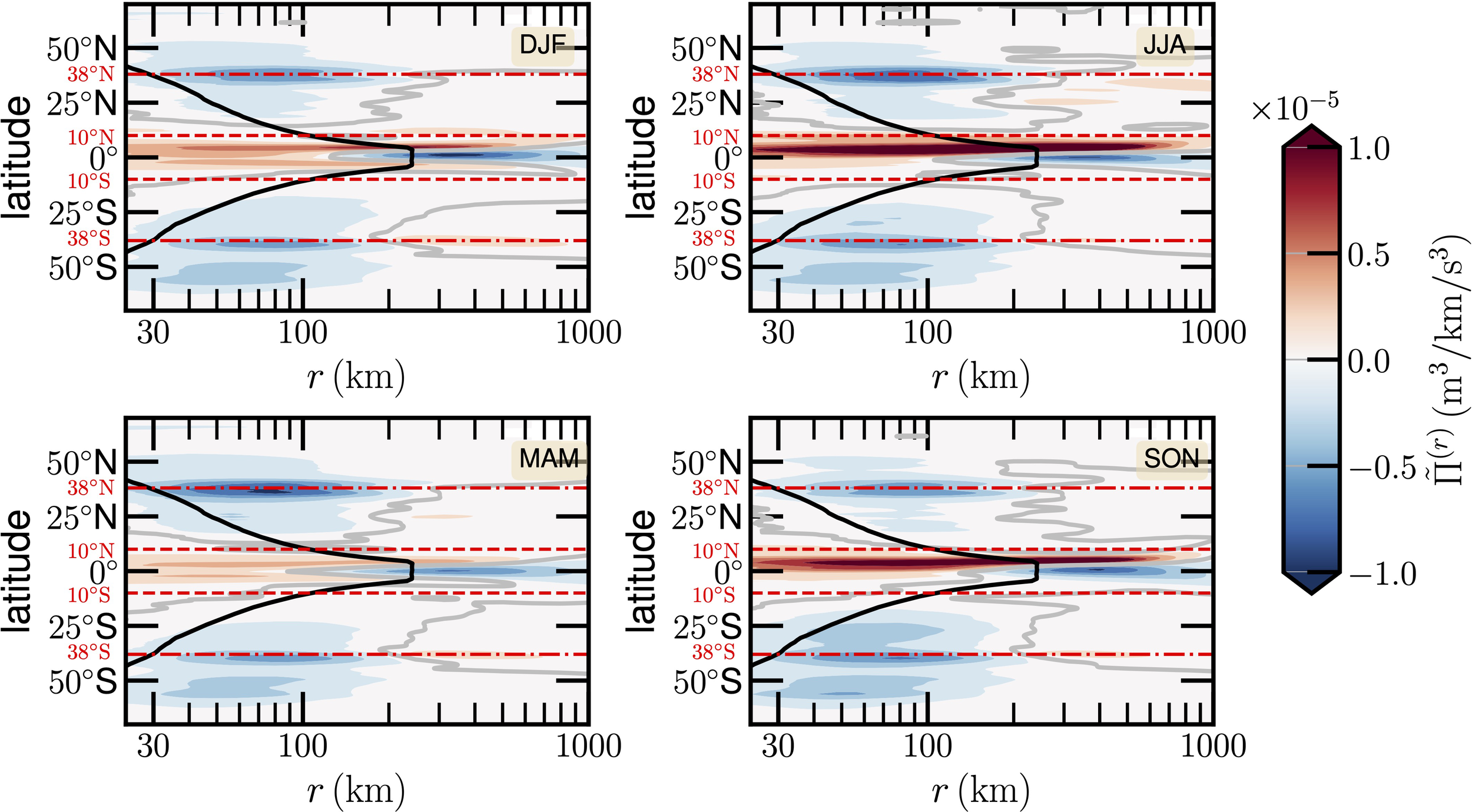
Figure 2 Longitude averaged energy flux ${\tilde{\Pi }}^{(r)}$ for four seasons. The separation between positive and negative ${\tilde{\Pi }}^{(r)}$ is indicated by a thick gray line, and the thick solid black line illustrates the latitude-average Rossby radius of deformation. The horizontal dashed red lines indicate the ECC region in the range 10°S-10°N. The dash-dotted red lines indicate the 38°S and 38°N for the high-intensity negative energy flux.

Figure 2 shows the longitudinally averaged energy fluxes ${\tilde{\Pi }}^{(r)}$ for four seasons, in which a thick gray line illustrates the separation between the positive and negative fluxes, and the longitude averaged Rossby radius r_R is indicated by a thick solid black line. Roughly speaking, despite the land coverage effect, it is symmetric with respect to the equator. For example, due to the existence of a strong WBCs, a negative value for ${\tilde{\Pi }}^{(r)}$ with nearly the same scale-latitude pattern is observed in the area 60°S-10°S, 10°N-60°N with minimum values at 38°S and 38°N, respectively. It suggests a strong inverse cascade owing to interactions between (mesoscale) eddies and the mainstream. It is also interesting to note that the computed ${\tilde{\Pi }}^{(r)}$ is strongly asymmetric in the ECC region. For instance, when r ≲ 100km, values in the North ECC are nearly 2 to 8 times larger than those in the south ECC. A high-intensity positive value is extended up to 800km in the North ECC with a tongue-like pattern, while on the contrary, a high-intensity negative value is observed when 100 ≲ r ≲ 800km. It suggests a strong forward cascade in the North, and an inverse cascade in the South. Indeed, several authors have reported the inverse cascade for laboratory experiments (Xia et al., 2011), Jupiter’s atmosphere (Young and Read, 2017), and oceanic flows (Scott and Wang, 2005; Aluie et al., 2018; Schubert et al., 2020; Garabato et al., 2022; Steinberg et al., 2022), to list a few. However, the situation for real atmospheric and oceanic flows is more complex with, for example, forcing at different spatial and temporal scales, earth rotation, and stratification, the real cascade could thus be a nonlinear superposition of direct and inverse cascades among a wide range of scales (Cencini et al., 2011). An elegant way to evaluate external forces is still needed to identify the exact mechanism (Balwada et al., 2022); more comments are provided in the discussion section. Moreover, a significant seasonal variation is observed. For example, in the JJA and SON, a stronger positive ${\tilde{\Pi }}^{(r)}$ for the ECC region is observed than those in DJF and MAM.

3.2 Typical regions

Based on the latitude-dependent ${\tilde{\Pi }}^{(r)}$ in Figure 2, four typical regions are considered here for further discussion. They are (a) the Kuroshio Current in the range 25°N-40°N and 120°E-160°E, (b) the Equatorial Counter Current in the Indian Ocean in the area 10°S-10°N and 60°E-100°E, (c) the Agulhas and Mozambique Current in the area 55°S-30°S and 30°E-90°E, and (d) the Equatorial Counter Current respectively in the areas 0°-10°N and 160°W-120°W, and 10°S-0° and 160°W-160°W, see Figure 3, where the background shows a time-averaged energy flux ${\tilde{\Pi }}^{(r)}$ with r ≃ 100km. These areas belong to WBCs or ECC, where strong current flows are evident (Hu et al., 2015; Todd et al., 2019; Hu et al., 2020). Other regions, such as the Loop Current, Brazil Current, the Luzon Strait, etc., might also be of great interest, and will be discussed in other works. Then a time series of the region-average ${\tilde{\Pi }}^{(r)}(t)$ is extracted. The time phase averaged ${\tilde{\Pi }}^{(r)}$ without time overlapping, the Pearson correlation coefficient ρ(r, τ) for different scales are then calculated for each region to emphasize the forward/inverse cascade, and the annual cycle due to the earth revolution. The Pearson correlation coefficient ρ(r, τ) is given as follows,

Figure 3

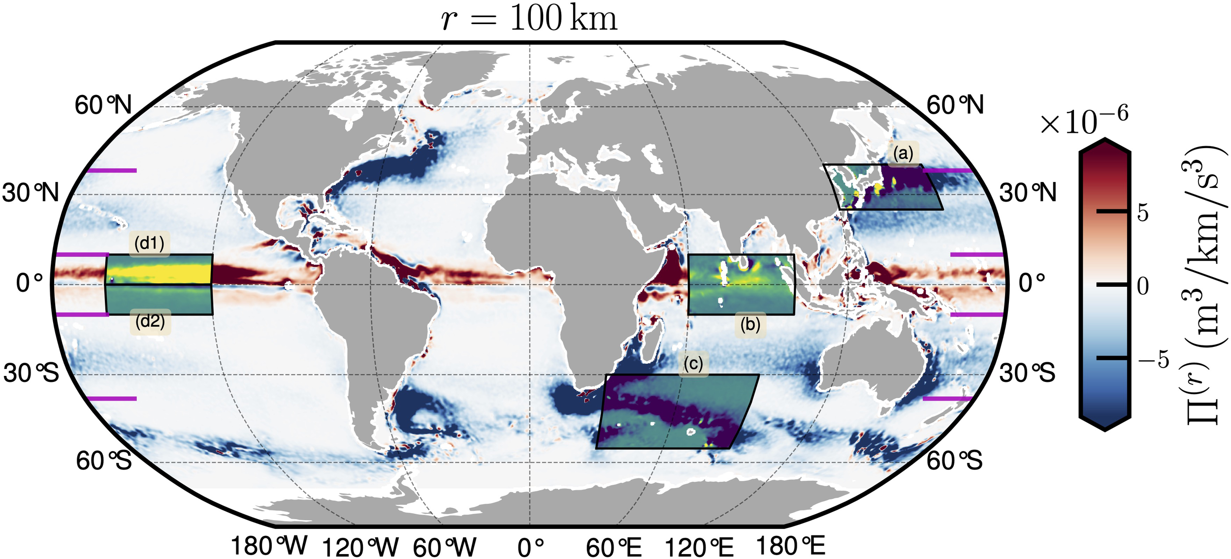
Figure 3 Four typical regions: (a) the Kuroshio Current in the area 25°N-40°N and 120°E-160°E, (b) the Equatorial Counter Current in Indian Ocean in the area 10°S-10°N and 60°E-100°E, (c) the Agulhas Current and the Mozambique Current in the area 55°S-30°S and 30°E-90°E, and (d) the Equatorial Counter Current respectively in the areas (d1) 0°-10°N and 160°W-120°W, and (d2) 10°S-0° and 160°W-120°W. The background is the time-averaged energy flux Π^(r) at r ≃ 100km. The horizontal solid lines indicates 38^◦S, 10°S, 10°N and 38°N, respectively.

$\begin{array}{ll}\rho (r,\tau )=\frac{\langle x^{\prime }(r,t)y^{\prime }(r,t+\tau )\rangle }{{\sigma }_x{\sigma }_y}& (7)\end{array}$

Where x^′(r,t) and y^′(r, t) are the centered region-average energy flux at the same (i.e., x = y) or two different locations (i.e., x ≠ y); ⟨·⟩ means average; σ is the standard deviation, and τ is the separation time scale.

3.2.1 The Kuroshio Current

The Kuroshio Current is a north-flowing warm current on the west side of the North Pacific Ocean basin. It is one of the strongest WBCs that transports warm equatorial water northward and forms the western limb of the North Pacific Subtropical Gyre. The Kuroshio Current has significant effects on both physical and biological processes of the North Pacific Ocean, including the transport of nutrients and sediments in the regional climate and the formation of Pacific mode water (Hu et al., 2015; Nagai et al., 2019). Moreover, it has been shown that the Kuroshio Current is closely associated with climate change (Chen et al., 2019). An area 25°N-40°N and 120°E-160°E is chosen to cover the main structure of the Kuroshio current, while the Luzon Strait is excluded occasionally without any specific reasons; see Figure 3. As shown previously, the scale-to-scale energy exchange activity in this area is intensive, see also Figure 1. To further see the seasonal variation, the time phase averaged energy flux is shown in the left panel of Figure 4. The inverse cascade, i.e., negative values of Π^(r), dominates when r ≲ 380km, while the forward cascade, that is, positive Π^(r), does dominate when r ≳ 380km. The highest intensity of the inverse cascade is found on the period of March to August of the year, e.g., corresponding to the boreal Springtime (March-May-April, MMA) and Summertime (June-July-August, JJA), indicating a strong seasonal variation. A typical spatial scale is found on the range 50 ≲ r ≲ 120km, which agrees well with the radius of the mesoscale eddy reported in this area (Jan et al., 2017; Sun et al., 2022). The inverse energy cascade found here means that the energy is transferred from these mesoscale eddies to larger scale motions, while the forward cascade transfers the energy from a much larger scale motion r ≫ 400km down to small scale ones. The separation scale between these two regimes is around r ≃ 380km, which is roughly 9 times of the Rossby radius.

Figure 4

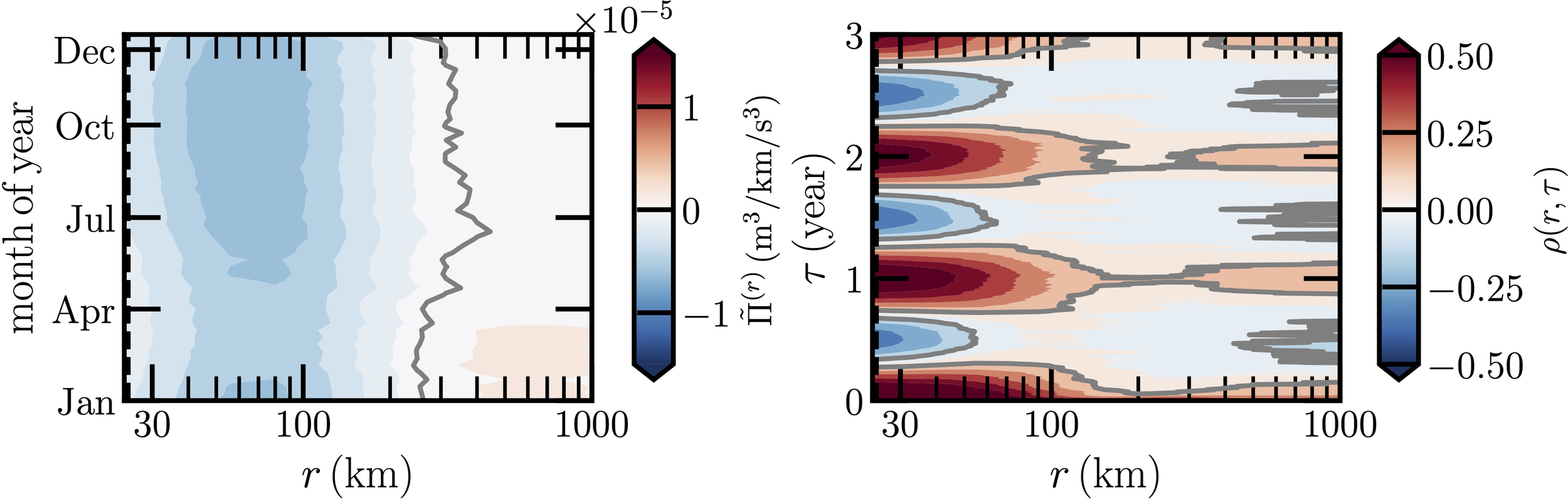
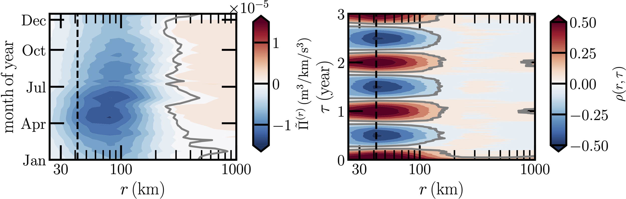
Figure 4 Left panel: The phase average ${\tilde{\Pi }}^{(r)}$ for Kuroshio Current, where ${\tilde{\Pi }}^{(r)}=0$ is indicated by a thick gray line. Right panel: Measured autocorrelation function ρ(r, τ) on the range 0 ≲ τ ≲ 3year to emphasize the annual cycle, where the thick gray line indicates the correlation value ρ(τ) = 0. The corresponding Rossby radius of deformation r_R = 42km is illustrated as a vertical dashed black line.

To emphasize the r-dependent annual cycle, the autocorrelation function ρ(r, τ) through the Equation (7) on the range of delay time 0 ≲ τ ≲ 3years is shown in the right panel of Figure 4, in which the value ρ(τ) = 0 is illustrated by a thick gray line. Visually, the annual cycle is clearly observed when r ≲ 100km. It suggests that mesoscale eddy activity has a strong annual cycle, while with increasing the spatial scale, large-scale structures feel less the Earth revolution, thus showing less seasonal variation when r ≳ 400km.

3.2.2 Equator Counter Current in the Indian Ocean

Unlike the North Equatorial Current (NEC) and the South Equatorial Current (SEC) where the surface flow is westward, the ECC is a major eastward surface flow in the Atlantic, Indian, and Pacific Oceans. Note that the other major surface currents in the tropic flow are in the same direction as the prevailing winds, while the flow direction of the ECC is in the opposite direction of the surface winds (Wyrtki and Kendall, 1967; Hermes et al., 2019). Moreover, due to the influence of the monsoon, there exists an eastward Equatorial Jet in the Indian Ocean, also known as the Wyrtki Jet, during the boreal spring (e.g., April to June) and fall (e.g., October to December) in the area 10°S-10°N and 60°E-90°E (Wyrtki, 1973; Hermes et al., 2019). To take this Wyrtki Jet into account, an area 10°S-10°N and 60°E-100°E is chosen, see Figure 3.

The time phase averaged energy flux ${\tilde{\Pi }}^{(r)}$ is shown in the left panel of Figure 5. Note that the scale-season pattern is quite different from the one for the Kuroshio Current, see Figure 4, where a clear seasonal variation is observed. Overall, both the Kuroshio Current and ECC regions share the same order of positive ${\tilde{\Pi }}^{(r)}$, while the negative value of the former one is nearly twice the latter one. Moreover, the annual cycle of this ECC is less notable. More precisely, a strong negative regime is observed in the period of February to March of year for the scale range from 300km up to at least 1200km. A high-intensity positive regime is found in the period of November to December of year for a scale range from 10km to 100km. The right panel of Figure 5 shows the measured ρ(r, τ). It confirms quantitatively that the annual cycle is less notable. It is interesting to see that the intensity of the annual cycle is first decreasing with r, and disappears around the Rossby radius, it is then increasing again with r when r ≳ 300km. These observations indicate a more complex dynamics than the one in the Kuroshio Current, partially due to the presence of the monsoon event.

Figure 5

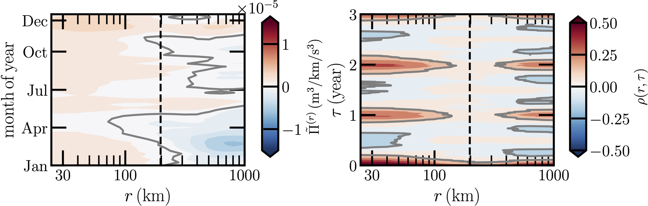
Figure 5 Same as Figure 4 but for the ECC in the Indian Ocean. The corresponding Rossby radius of deformation r_R = 200km is illustrated as a vertical dashed black line.

3.2.3 Agulhas and Mozambique Currents

Agulhas Current is a WBCs of the southern Indian Ocean that flows southward along the southeast coast of Mozambique and the coast of South Africa before turning eastward to join the flow from Africa to Australia (Lutjeharms, 2007; Beal and Elipot, 2016). The Mozambique Current, between Madagascar and Africa, also feeds the Agulhas Current. In the South of Madagascar, both streams feed into the Agulhas Current. The area 55°S-30°S and 30°E-90°E is considered here, in which the Agulhas rings/mesoscale eddiess are also covered (van Leeuwen et al., 2000).

Figure 6 shows the time phase average ${\tilde{\Pi }}^{(r)}$, where the Rossby radius r_d = 25km is illustrated in the left of the figure. A dual cascade is observed, e.g., a high-intensity negative value is found on the range 30 ≲ r ≲ 120km with a minimum value at spatial scale r ≃ 60km, which agrees with the result obtained in Schubert et al. (2020), as well as with the radius of mesoscale eddies reported in the literature (Chelton et al., 2011; Casanova-Masjoan et al., 2017; Gulliver and Radko, 2022). The mean separation scale between the negative and positive ${\tilde{\Pi }}^{(r)}$ is around 290km. Above this scale, a strong positive value is found for January to March of year and on the range 400-1100km. The measured ρ(r, τ) confirms the existence of the annual cycle when r ≲ 200km, and a weak one when r ≳ 300km.

Figure 6

Figure 6 Same as Figure 4 but for the Agulhas and Mozambique Currents. The corresponding Rossby radius of deformation r_R = 25km is illustrated as a vertical dashed black line, which is close to the left edge of the figure.

3.2.4 Equatorial Counter Current in the Pacific Ocean

As aforementioned, the ECC is a strong surface current that is in the opposite direction of the surface winds (Knauss, 1961; Wyrtki and Kendall, 1967). It is also found that the ECC in the Pacific Ocean is deeply associated with the climate system, such as El Niño (Tan and Zhou, 2018; Zhou et al., 2021). To see the possible difference between the Northern and Southern Hemispheres, two regions are chosen, they are in the areas 0°-10°N and 10°S-0° with longitude on the range 160°W-120°W, see Figure 3.

The left panel of Figure 7 shows the time phase average ${\tilde{\Pi }}^{(r)}$. Visually, they show different patterns. For instance, when r ≲ 200km, a high-intensity positive region of the North ECC for July to December of year is found to be 10 times larger than the one in South ECC. In comparison with the positive ${\tilde{\Pi }}^{(r)}$, a relative weak ${\tilde{\Pi }}^{(r)}$ is found when r ≳ 200km for January to May of year. While in the South ECC, when r ≳ 100km, it is dominated by the inverse energy cascade. However, the annual cycle is less notable for both of them, see the right panel of Figure 7.

Figure 7

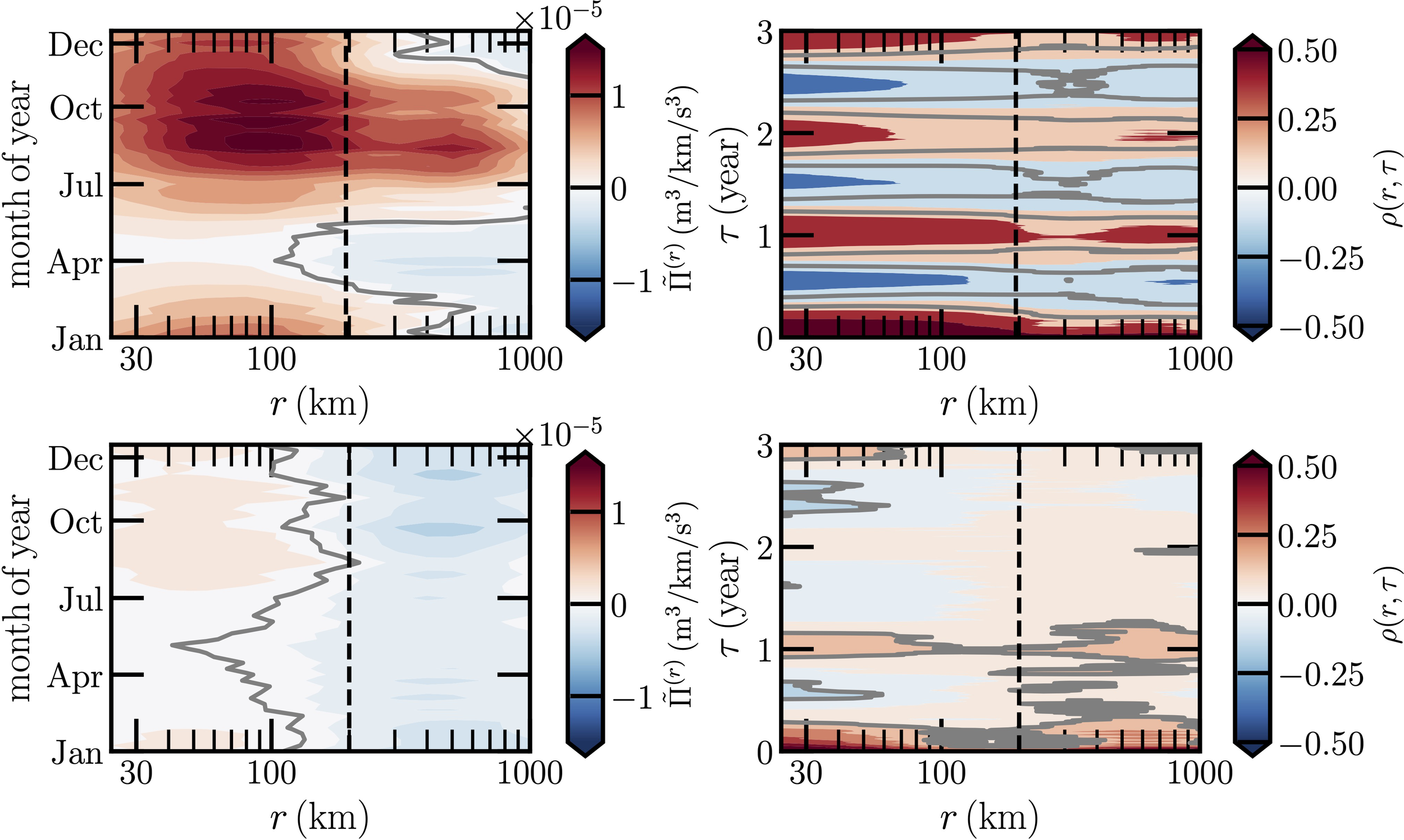
Figure 7 Same as Figure 4 but for the ECC in the Pacific Ocean: top row (d1) is for North ECC and bottom row (d2) for the South ECC. The corresponding Rossby radius of deformation r_R = 200km is illustrated as a vertical dashed black line.

To check the naive relation between the North and South ECC, a scale-to-scale cross-correlation ρ(r_N, r_S) is then calculated, see Figure 8. It is interesting to note that this phase diagram could be divided into four sections. In section (a), r_N, r_S ≲ 200km, they are in-phase correlated with a highest correlation coefficient of value ρ(r_N, r_S) = 0.6. With the increase of r_N, it is gradually decreasing to 0.2 ≲ ρ(r_N, r_S) ≲ 0.3 in the section (b). If one keeps r_N ≲ 200km, and with the increase of r_S, it reaches an out-of-phase correlated regime with a minimum correlation coefficient of value ρ(r_N, r_S) = −0.28 in the section (d), while in section (c), it is first in the out-of-phase (e.g., negatively correlated) regime, and then transits to the in-phase (e.g., positively correlated) regime.

Figure 8

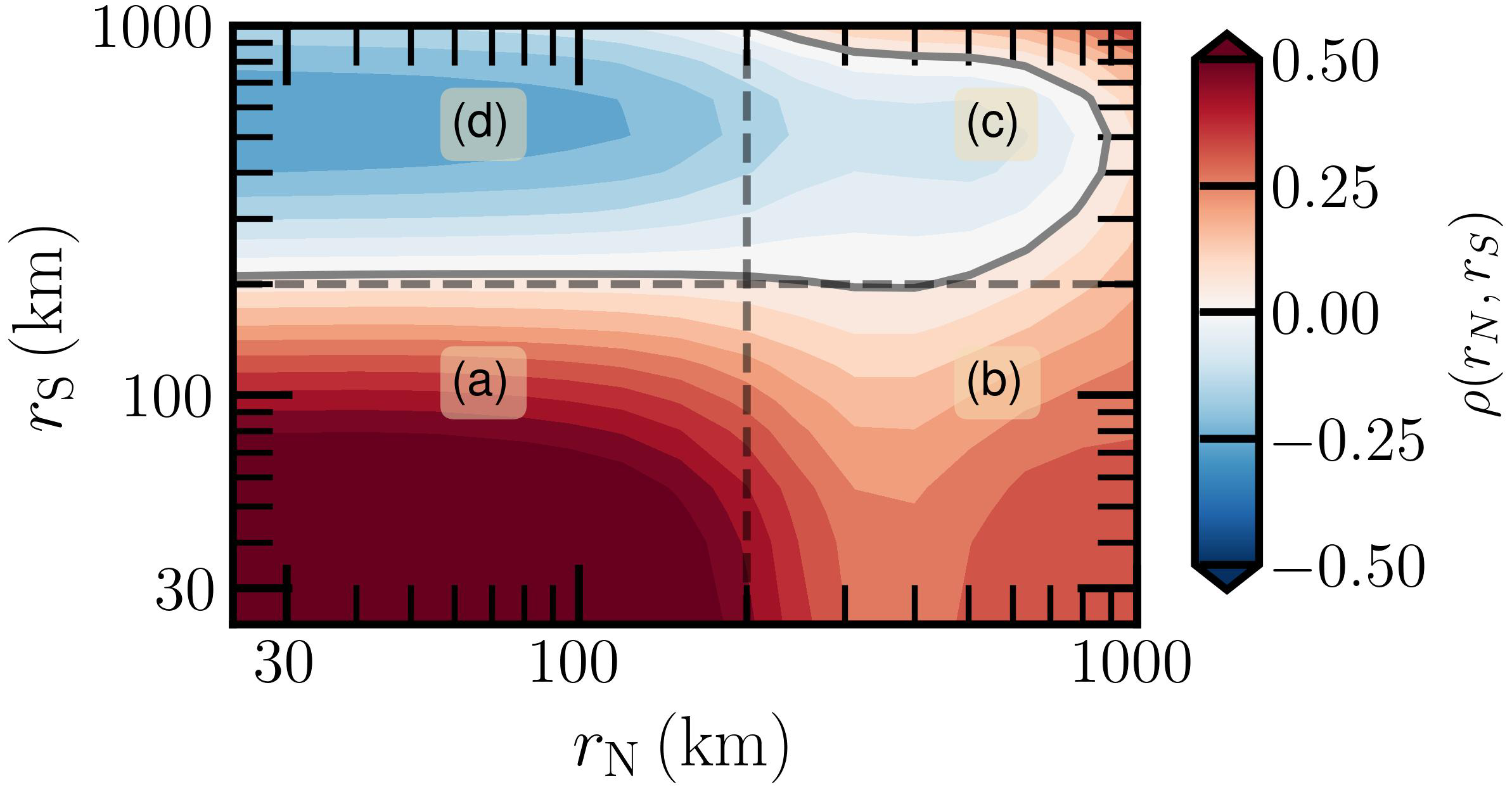
Figure 8 Experimental scale-to-scale correlation ρ(r_N, r_S) between (d1-r_N) and (d2-r_S), where the corresponding Rossby radius of deformation r_R = 200km is illustrated as dashed black lines. The zero correlation ρ(r_N, r_S) = 0 is indicated by a thick gray line. They are divided into four regimes by the Rossby radius as (A–D).

4 Discussions and conclusions

As aforementioned, the concept of the forward energy cascade advocated by Richardson 100 years ago was first used to describe the complex movement of the atmosphere phenomenologically (Richardson, 1922). The forward energy cascade in 3D turbulent flows was then quantitatively described by the Kolmogorov theory in 1941 (Kolmogorov, 1941b; Frisch, 1995; Schmitt and Huang, 2016). At the same time, Chou (1940), Chou (1945) first developed a method to close the Reynolds-Average-Navier-Stokes equations. Later, the inverse energy cascade was then generalized by Kraichnan (1967) to cope with the 2D case of turbulence, where the energy could be transferred inversely from small-scale structures to larger-scale ones. The idea of forward and inverse energy cascades, is now widely accepted. They are also the root of the geophysical flow modelling (Slingo et al., 2009, 2021), e.g., the Global Circulation Model (GCM), Regional Ocean Modeling System (ROMS), etc. However, the situation is more complex than the ideal flows since, for instance, geometric constraints (e.g., quasi-2D, complex boundaries), stratification, earth rotation/Coriolis force, complex external forces, are present. The efficient scale-to-scale energy flux diagnosis method is still needed to determine quantitatively both the strength and direction of the cascade in either the observed velocity field or the output of those models. While these three different methodologies derived from the Navier-Stokes equations offer potential for analyzing cross-scale energy transfer, each presents limitations for real-world oceanic and atmospheric flows. For instance, the application of the classical third-order structure-function of Equation (1) needs the a priori knowledge of external forcing, which is often unavailable for complex natural flows. The spectral representation of Equation (2) provides a global representation of the cross-scale energy transfer, but necessitates a regular domain without missing data, rendering it unsuitable for irregular ocean boundaries. The Filter-Space Technique emerges as a promising candidate, addressing these constraints and offering distinct advantages: it reveals scale-to-scale energy flux at specific locations, crucial for understanding localized dynamics in oceanic and atmospheric systems.

When applying this method to the CMEMS reanalysis data, both forward and inverse energy cascades are observed. Globally, it shows a strong latitude dependence partially due to the Coriolis force/earth rotation. The high-intensity inverse cascade is mainly found in the WBCs, where the mesoscale eddy is abundant. In other words, the fate of the mesoscale eddy is likely absorbed by the mainstream during the eddy-mainstream interaction. A high-intensity cascade is also found in the ECC, where a strong asymmetric pattern is visible with a tongue-like pattern. It is dominated by the forward cascade when the scale is below the Rossby radius, while dominated by the inverse cascade when the scale is above the Rossby radius, see Figure 2. Note that the inverse cascade is an important mechanism to maintain the large-scale motions (Young and Read, 2017; Dong et al., 2020).

Furthermore, it is not always true that all scale motions can feel the Earth’s revolution, and thus possess a clear annual cycle. The preliminary results presented in this work show that it is highly dependent on spatial scales and regions. For example, it is evident in the case of the Kuroshio Current when r ≲ 200km, while is less visible in the South ECC of the Pacific Ocean for all scales. However, for the case of the Indian Ocean, it is interesting to note that the annual cycle is detected both below and above the Rossby radius. All these preliminary results show an extremely dynamic oceanic flow. More detailed analysis should be performed region-by-region to highlight the local dynamics.

One might to estimate the external forcing via the local energy balance analysis as follows. Assuming the statistical stationarity, one has the following relation for the local energy balance (Frisch, 1995),

$\begin{array}{ll}{\text{d}}_r{\Pi }^{(r)}={ϵ}_v(r)-E_{\text{in}}(r)& (8)\end{array}$

where ϵ_ν(r) is the energy dissipation density function due to the fluid viscosity, while E_in(r) denotes the energy injection density function resulting from external forces or other interactions. It is worth noting that ϵ_ν(r) must be greater than or equal to zero, and it approaches zero for scales significantly larger than the viscosity scale (e.g., few millimeters in the ocean). In our case, it is safe to assume ϵ_ν(r) ≃ 0. The above Equation (8) is then simplified as follows,

$\begin{array}{ll}{\text{d}}_r{\Pi }^{(r)}\simeq -E_{in}(r)& (9)\end{array}$

Therefore, by definition, the negative ${\text{d}}_r{\Pi }^{(r)}$ indicates an energy injection into the loop of the energy cascade and vice versa. Figure 9 shows the longitudinal-average ${\text{d}}_r{\tilde{\Pi }}^{(r)}$ estimated from Equation (9) for different seasons, where the Rossby deformation radius is illustrated by a solid black line, and the value ${\text{d}}_r{\tilde{\Pi }}^{(r)}=0$ is illustrated by a gray line. It is interesting to see that high negative values of ${\text{d}}_r{\tilde{\Pi }}^{(r)}$ appear near the Rossby radius of deformation when r ≲ 70 km, indicating a strong interaction between the mesoscale eddy and the Coriolis force in the middle latitudes. Positive values of ${\text{d}}_r{\tilde{\Pi }}^{(r)}$ mean that energy is taken out of the loop of the energy cascade, mostly as a result of the out-phase interaction between the large flow structure and the Coriolis force or the air-sea interaction. This pattern has been observed for several different types of quasi-two-dimensional turbulent systems, in which the inverse energy cascade is relevant. Moreover, the trend in the equatorial area is the opposite: with an increase of scales, it is first positive and then approaches a negative regime with a strong seasonal variation.

Figure 9

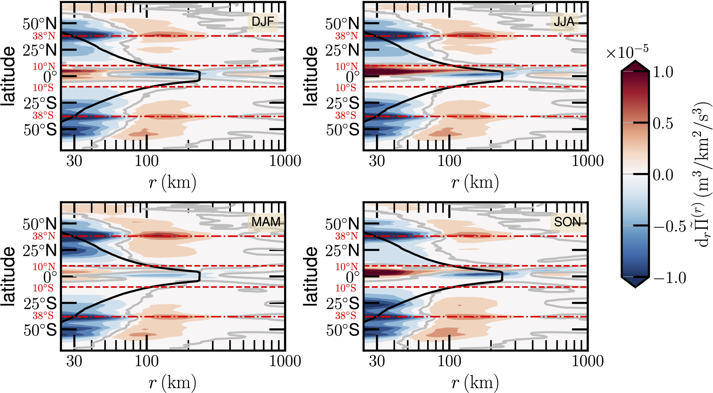
Figure 9 Longitudinal average d_rΠ^(r) for four seasons, where the Rossby radius of deformation is illustrated as a solid black line. The value d_rΠ^(r) = 0 is illustrated as a thick gray line.

Future exploration of energy transfer efficiency holds promise for advancing our understanding of oceanic flows. As highlighted in Refs (Xiao et al., 2009; Fang and Ouellette, 2016; De Leo and Stocchino, 2023), quantifying this efficiency can illuminate the mechanisms governing energy transport across scales. Central to this analysis is the relationship between the turbulent stress tensor ${\tau }_{ij}^{(r)}={(u_i{u}_j)}^{(r)}-u_i^{(r)}{u}_j^{(r)}$ and the strain rate tensor $S_{ij}^{(r)}=\frac{1}{2}\left(\partial u_i^{(r)}/\partial x_j+\partial u_j^{(r)}/\partial x_i\right)$ of the coarse-grained velocity field. The scale-to-scale energy flux defined in Equation (5) can be rewritten as follow,

$\begin{array}{ll}{\Pi }^{(r)}=-{\tau }_{ij}^{(r)}{S}_{ij}^{(r)}& (10)\end{array}$

Crucially, the Equation (10) can be further decomposed to reveal the role of eigenvalue alignment, which is written as,

$\begin{array}{ll}{\Pi }^{(r)}=-{\lambda }_{\tau }^{(r)}{\lambda }_S^{(r)}\cos \left(2{\text{Θ}}_{\Pi }^{(r)}\right)& (11)\end{array}$

Here, ${\lambda }_{\tau }^{(r)}$ and ${\lambda }_S^{(r)}$ denote the maximum eigenvalues of the respective tensors, while ${\text{Θ}}_{\Pi }^{(r)}$ represents the angle between their corresponding eigenvectors. For example, when ${\text{Θ}}_{\Pi }^{(r)}=0$, the turbulent stress and strain rate are perfectly aligned and yields an efficiency of 1, signifying maximum energy transfer towards larger scales (inverse energy cascade); when ${\text{Θ}}_{\Pi }^{(r)}=\pi /2$, the turbulent stress perfectly aligns with the compressive strain-rate eigenvector and yields an efficiency of −1, indicating maximum energy transfer towards smaller scales (forward energy cascade). These insights will underscore the potential for investigating energy transfer efficiency through the Equation (11) to uncover fundamental principles governing oceanic dynamics.

It is worth pointing out that the dynamics of the real oceanic flow could be different from what is produced by GCM models. This is because the cascade in turbulence-like systems is highly nonlinear and sensitive to external force, boundary conditions, etc (Sérazin et al., 2018). In the GCM model, the external force (e.g., input of the kinetic energy) and the dissipation mechanism (e.g. dissipation of the kinetic energy) are assumed a priori. Moreover, the scale-to-scale flux depends on the phase information of the velocity vector and its spatial gradients, see definition in Equation (5). Although, it has been shown experimentally that the FST method is robust with different spatial resolutions (Ni et al., 2014). However, the experimental energy flux might depend on the time resolution. For example, the mean energy flux for r = 200km provided by the monthly mean velocity field is roughly half of those provided by the daily mean velocity field (figure not shown here). The spatial range provided by the observation is limited; for example, the one from the ocean surface wind velocity field provided by the high-frequency radar is at 𝒪(1)km to 𝒪(100)km (Roarty et al., 2019), and by the satellite is at 𝒪(10)km to 𝒪(1000)km [e.g., 12.5km to 1050km for the China France Oceanography SATellite (CFOSAT) data (Hauser et al., 2020)]. However, it is still a challenge to measure a large area of the oceanic flow field with a high spatial and temporal resolution to verify the whole picture of cascade from 3D (e.g., a few millimeters to hundreds of meters) to a quasi-2D case, e.g, submesoscale dynamics (e.g., from hundreds of meters to few kilometers), and mesoscale eddies (dozen of kilometers to few hundreds of kilometers), even to the oceanic circulations. Hopefully, with the increasing capability of observation and computation, such data will be accessible in the near future.

In summary, taking the irregular domain into account, the Filter-Space-Technique, also known as Coarse-Graining, is applied to the CMEMS reanalysis data to provide a global view of the scale-to-scale energy flux, which is the key point for understanding cascading dynamics. The preliminary results show clear evidence of both inverse and forward energy cascades (Balwada et al., 2022; Qiu et al., 2022); see Figure 2 and the movie in the Supplementary Material. It seems that the high-intensity inverse cascade is deeply associated with the dynamics of mesoscale eddies, especially in WBCs, indicating that the fate of the mesoscale eddy might be absorbed by the mainstream. The situation of the ECC in the Pacific Ocean seems to be more complex. For instance, below the Rossby radius, the scale-to-scale flux is in-phase correlated, while above this scale, it is out-phase, showing very complex dynamics.

Data availability statement

The original contributions presented in the study are included in the article/Supplementary Material. Further inquiries can be directed to the corresponding author. A copy of Python codes to perform the analyses presented in this work can be found at https://github.com/lanlankai/Filter-Sapce-Technique-via-FFT.

Author contributions

DZ: Investigation, Supervision, Writing – review & editing. JS: Data curation, Writing – review & editing. YG: Data curation, Writing – review & editing. YP: Writing – review & editing. JH: Investigation, Writing – review & editing. FS: Investigation, Writing – review & editing. YH: Conceptualization, Investigation, Supervision, Writing – review & editing.

Funding

The author(s) declare financial support was received for the research, authorship, and/or publication of this article. This work was supported by the National Natural Science Foundation of China (61973208, 91958203, 11732010, 41876004, U22A20579). This research has been also done in the frame of the Multiw2 project funded by the CNES/TOSCA program. Funding of YG’s Cotutella doctoral research project by Region´ Hauts-de-France and Xiamen University is acknowledged. YH is partially supported by the State Key Laboratory of Ocean Engineering (Shanghai Jiao Tong University) (Grant No. 1910).

Acknowledgments

We thank CMEMS for providing the nice reanalysis data. We would like to dedicate this work to the 100th Anniversary of Richardson’s idea of cascades.

Conflict of interest

The authors declare that the research was conducted in the absence of any commercial or financial relationships that could be construed as a potential conflict of interest.

The author(s) declared that they were an editorial board member of Frontiers, at the time of submission. This had no impact on the peer review process and the final decision.

Publisher’s note

All claims expressed in this article are solely those of the authors and do not necessarily represent those of their affiliated organizations, or those of the publisher, the editors and the reviewers. Any product that may be evaluated in this article, or claim that may be made by its manufacturer, is not guaranteed or endorsed by the publisher.

Supplementary material

A movie showing the time evolution of the scale-to-scale energy flux at scales 100, 200, 500, and 1000km can be found in the Supplementary Material for this article online at: https://www.frontiersin.org/articles/10.3389/fmars.2024.1307751/full#supplementary-material.

References

Alexakis A., Biferale L. (2018). Cascades and transitions in turbulent flows. Phys. Rep. 767, 1–101. doi: 10.1016/j.physrep.2018.08.001

CrossRef Full Text | Google Scholar

Aluie H. (2019). Convolutions on the sphere: Commutation with differential operators. GEM-International J. Geomathematics 10, 1–31. doi: 10.1007/s13137-019-0123-9

CrossRef Full Text | Google Scholar

Aluie H., Hecht M., Vallis G. K. (2018). Mapping the energy cascade in the north Atlantic Ocean: The coarse-graining approach. J. Phys. Oceanography 48, 225–244. doi: 10.1175/JPO-D-17-0100.1

CrossRef Full Text | Google Scholar

Aluie H., Kurien S. (2011). Joint downscale fluxes of energy and potential enstrophy in rotating stratified Boussinesq flows. EPL (Europhysics Letters) 96, 44006. doi: 10.1209/0295-5075/96/44006

CrossRef Full Text | Google Scholar

Bai K., Meneveau C., Katz J. (2013). Experimental study of spectral energy fluxes in turbulence generated by a fractal, tree-like object. Phys. Fluids 25, 110810. doi: 10.1063/1.4819351

CrossRef Full Text | Google Scholar

Balwada D., Xie J.-H., Marino R., Feraco F. (2022). Direct observational evidence of an oceanic dual kinetic energy cascade and its seasonality. Sci. Adv. 8, eabq2566. doi: 10.1126/sciadv.abq2566

PubMed Abstract | CrossRef Full Text | Google Scholar

Barkan R., Srinivasan K., Yang L., McWilliams J. C., Gula J., Vic C. (2021). Oceanic mesoscale eddy depletion catalyzed by internal waves. Geophysical Res. Lett. 48, e2021GL094376. doi: 10.1029/2021GL094376

CrossRef Full Text | Google Scholar

Beal L. M., Elipot S. (2016). Broadening not strengthening of the Agulhas Current since the early 1990s. Nature 540, 570–573. doi: 10.1038/nature19853

PubMed Abstract | CrossRef Full Text | Google Scholar

Beck A., Kurz M. (2021). A perspective on machine learning methods in turbulence modeling. GAMM-Mitteilungen 44, e202100002. doi: 10.1002/gamm.202100002

CrossRef Full Text | Google Scholar

Boffetta G., Ecke R. (2012). Two-dimensional turbulence. Annu. Rev. Fluid Mechanics 44, 427–451. doi: 10.1146/annurev-fluid-120710-101240

CrossRef Full Text | Google Scholar

Buzzicotti1 M., Storer B. A., Griffies S., Aluie H. (2021). A coarse-grained decomposition of surface geostrophic kinetic energy in the global ocean. ESS Open Arch. doi: 10.1002/essoar.10507290.1

CrossRef Full Text | Google Scholar

Casanova-Masjoan M., Pelegrí J. L., Sangrà P., Martínez A., Grisolía-Santos D., Pérez-Hernández M. D., et al. (2017). Characteristics and evolution of an Agulhas ring. J. Geophysical Research: Oceans 122, 7049–7065. doi: 10.1002/2015JC011620

CrossRef Full Text | Google Scholar

Cencini M., Muratore-Ginanneschi P., Vulpiani A. (2011). Nonlinear superposition of direct and inverse cascades in two-dimensional turbulence forced at large and small scales. Phys. Rev. Lett. 107, 174502. doi: 10.1103/PhysRevLett.107.174502

PubMed Abstract | CrossRef Full Text | Google Scholar

Charney J. G. (1971). Geostrophic turbulence. J. Atmospheric Sci. 28, 1087–1095. doi: 10.1175/1520-0469(1971)028<1087:GT>2.0.CO;2

CrossRef Full Text | Google Scholar

Chassignet E. P., Xu X. (2017). Impact of horizontal resolution (1/12 to 1/50) on Gulf Stream separation, penetration, and variability. J. Phys. Oceanography 47, 1999–2021. doi: 10.1175/JPO-D-17-0031.1

CrossRef Full Text | Google Scholar

Chelton D. B., DeSzoeke R. A., Schlax M. G., El Naggar K., Siwertz N. (1998). Geographical variability of the first baroclinic Rossby radius of deformation. J. Phys. Oceanography 28, 433–460. doi: 10.1175/1520-0485(1998)028<0433:GVOTFB>2.0.CO;2

CrossRef Full Text | Google Scholar

Chelton D. B., Schlax M. G., Samelson R. M. (2011). Global observations of nonlinear mesoscale eddies. Prog. Oceanography 91, 167–216. doi: 10.1016/j.pocean.2011.01.002

CrossRef Full Text | Google Scholar

Chen C., Wang G., Xie S.-P., Liu W. (2019). Why does global warming weaken the Gulf Stream but intensify the Kuroshio? J. Climate 32, 7437–7451. doi: 10.1175/JCLI-D-18-0895.1

CrossRef Full Text | Google Scholar

Chen S., Ecke R., Eyink G., Rivera M., Wan M., Xiao Z. (2006). Physical mechanism of the two-dimensional inverse energy cascade. Phys. Rev. Lett. 96, 84502. doi: 10.1103/PhysRevLett.96.084502

CrossRef Full Text | Google Scholar

Chou P. Y. (1940). On an extension of Reynolds’ method of finding apparent stress and the nature of turbulence. Chin. J. Phys. 4, 1–33.

Google Scholar

Chou P. Y. (1945). On velocity correlations and the solutions of the equations of turbulent fluctuation. Q. Appl. Mathematics 3, 38–54. doi: 10.1090/qam/1945-03-01

CrossRef Full Text | Google Scholar

Contreras M., Renault L., Marchesiello P. (2023). Understanding energy pathways in the Gulf Stream. J. Phys. Oceanography 53, 719–736. doi: 10.1175/JPO-D-22-0146.1

CrossRef Full Text | Google Scholar

Davidson P. A. (2004). Turbulence: An Introduction for Scientists and Engineers (Oxford, UK: Oxford University Press). doi: 10.1093/acprof:oso/9780198722588.001.0001

CrossRef Full Text | Google Scholar

De Leo A., Stocchino A. (2022). Evidence of transient energy and enstrophy cascades in tidal flows: A scale to scale analysis. Geophysical Res. Lett. 49, e2022GL098043. doi: 10.1029/2022GL098043

CrossRef Full Text | Google Scholar

De Leo A., Stocchino A. (2023). Efficiency of energy and enstrophy transfers in periodical flows. Phys. Fluids 35. doi: 10.1063/5.0142848

CrossRef Full Text | Google Scholar

Dong S., Huang Y., Yuan X., Lozano-Durán A. (2020). The coherent structure of the kinetic energy transfer in shear turbulence. J. Fluid Mechanics 892, A22. doi: 10.1017/jfm.2020.195

CrossRef Full Text | Google Scholar

Evans D., Frajka-Williams E., Garabato A. N. (2022). Dissipation of mesoscale eddies at a western boundary via a direct energy cascade. Sci. Rep. 12:887 doi: 10.1038/s41598-022-05002-7

PubMed Abstract | CrossRef Full Text | Google Scholar

Eyink G. L. (2005). Locality of turbulent cascades. Physica D: Nonlinear Phenomena 207, 91–116. doi: 10.1016/j.physd.2005.05.018

CrossRef Full Text | Google Scholar

Fang L., Ouellette N. T. (2016). Advection and the efficiency of spectral energy transfer in twodimensional turbulence. Phys. Rev. Lett. 117, 104501. doi: 10.1103/PhysRevLett.117.104501

PubMed Abstract | CrossRef Full Text | Google Scholar

Frisch U. (1995). Turbulence: the legacy of AN Kolmogorov (Cambridge, UK: Cambridge University Press). doi: 10.1017/CBO9781139170666

CrossRef Full Text | Google Scholar

Gao Y. (2022). Scaling and coupling analysis of the wind speed and wave height, using CFOSAT and other satellites (Xiamen, China: Ph.D. thesis, Universite´ du Littoral Côte d’Opale and Xiamen University).

Google Scholar

Garabato A. C. N., Yu X., Callies J., Barkan R., Polzin K. L., Frajka-Williams E. E., et al. (2022). Kinetic energy transfers between mesoscale and submesoscale motions in the open ocean’s upper layers. J. Phys. Oceanography 52, 75–97. doi: 10.1175/JPO-D-21-0099.1

CrossRef Full Text | Google Scholar

Grooms I., Loose N., Abernathey R., Steinberg J. M., Bachman S. D., Marques G., et al. (2021). Diffusion-based smoothers for spatial filtering of gridded geophysical data. J. Adv. Modeling Earth Syst. 13, e2021MS002552. doi: 10.1029/2021MS002552

CrossRef Full Text | Google Scholar

Gulliver L., Radko T. (2022). Topographic stabilization of ocean rings. Geophysical Res. Lett. 49, e2021GL097686. doi: 10.1029/2021GL097686

CrossRef Full Text | Google Scholar

Hauser D., Tourain C., Hermozo L., Alraddawi D., Aouf L., Chapron B., et al. (2020). “New observations from the SWIM radar on-board CFOSAT: instrument validation and ocean wave measurement assessment,” in IEEE Transactions on Geoscience and Remote Sensing. 59(1):1–22. doi: 10.1109/TGRS.2020.2994372

CrossRef Full Text | Google Scholar

Hermes J. C., Masumoto Y., Beal L., Roxy M. K., Vialard J., Andres M., et al. (2019). A sustained ocean observing system in the Indian Ocean for climate related scientific knowledge and societal needs. Front. Mar. Sci. 6:355. doi: 10.3389/fmars.2019.00355

CrossRef Full Text | Google Scholar

Hewitt H. T., Roberts M., Mathiot P., Biastoch A., Blockley E., Chassignet E. P., et al. (2020). Resolving and parameterising the ocean mesoscale in earth system models. Curr. Climate Change Rep. 6, 137–152. doi: 10.1007/s40641-020-00164-w

CrossRef Full Text | Google Scholar

Hu D., Wu L., Cai W., Gupta A. S., Ganachaud A., Qiu B., et al. (2015). Pacific western boundary currents and their roles in climate. Nature 522, 299–308. doi: 10.1038/nature14504

PubMed Abstract | CrossRef Full Text | Google Scholar

Hu S., Sprintall J., Guan C., McPhaden M. J., Wang F., Hu D., et al. (2020). Deep-reaching acceleration of global mean ocean circulation over the past two decades. Sci. Adv. 6, eaax7727. doi: 10.1126/sciadv.aax772

PubMed Abstract | CrossRef Full Text | Google Scholar

Jan S., Mensah V., Andres M., Chang M.-H., Yang Y. J. (2017). Eddy-Kuroshio interactions: Local and remote effects. J. Geophysical Research: Oceans 122, 9744–9764. doi: 10.1002/2017JC013476

CrossRef Full Text | Google Scholar

Khatri H., Sukhatme J., Kumar A., Verma M. K. (2018). Surface ocean enstrophy, kinetic energy fluxes, and spectra from satellite altimetry. J. Geophysical Research: Oceans 123, 3875–3892. doi: 10.1029/2017JC013516

CrossRef Full Text | Google Scholar

Knauss J. A. (1961). The structure of the pacific equatorial countercurrent. J. Geophysical Res. 66, 143–155. doi: 10.1029/JZ066i001p00143

CrossRef Full Text | Google Scholar

Kolmogorov A. N. (1941a). Energy dissipation in locally isotropic turbulence. Doklady Akademii Nauk SSSR 32, 19–21.

Google Scholar

Kolmogorov A. N. (1941b). Local structure of turbulence in an incompressible fluid at very high Reynolds numbers. Doklady Akademii Nauk SSSR 30, 301–304.

Google Scholar

Kraichnan R. (1967). Inertial ranges in two-dimensional turbulence. Phys. Fluids 10, 1417–1423. doi: 10.1063/1.1762301

CrossRef Full Text | Google Scholar

Kraichnan R., Montgomery D. (1980). Two-dimensional turbulence. Rep. Prog. Phys. 43, 547. doi: 10.1088/0034-4885/43/5/001

CrossRef Full Text | Google Scholar

Landau L., Lifshits E. (1987). Fluid Mechanics (Pergamon, London: Elsevier, Oxford, UK).

Google Scholar

Leonard A. (1975). Energy cascade in large-eddy simulations of turbulent fluid flows. Adv. Geophysics 18, 237–248. doi: 10.1016/S0065-2687(08)60464-1

CrossRef Full Text | Google Scholar

Loose N., Bachman S., Grooms I., Jansen M. (2023). Diagnosing scale-dependent energy cycles in a high-resolution isopycnal ocean model. J. Phys. Oceanography 53, 157–176. doi: 10.1175/JPO-D-22-0083.1

CrossRef Full Text | Google Scholar

Lovejoy S. (2019). Weather, Macroweather, and the Climate: Our Random Yet Predictable Atmosphere (Cambridge, UK: Oxford University Press). doi: 10.1093/oso/9780190864217.001.0001

CrossRef Full Text | Google Scholar

Lutjeharms J. (2007). Three decades of research on the greater Agulhas Current. Ocean Sci. 3, 129–147. doi: 10.5194/os-3-129-2007

CrossRef Full Text | Google Scholar

Nagai T., Saito H., Suzuki K., Takahashi M. (2019). Kuroshio Current: Physical, Biogeochemical, and Ecosystem Dynamics Vol. 243 (Washington, D.C., USA: John Wiley & Sons). doi: 10.1002/9781119428428

CrossRef Full Text | Google Scholar

Nastrom G. D., Gage K. S., Jasperson W. H. (1984). Kinetic energy spectrum of large-and mesoscale atmospheric processes. Nature 310, 36–38. doi: 10.1038/310036a0

CrossRef Full Text | Google Scholar

Ni R., Voth G., Ouellette N. (2014). Extracting turbulent spectral transfer from under-resolved velocity field. Phys. Fluids 26, 105107. doi: 10.1063/1.4898866

CrossRef Full Text | Google Scholar

Pope S. (2000). Turbulent Flows (Cambridge, UK: Cambridge University Press). doi: 10.1088/0957-0233/12/11/705

CrossRef Full Text | Google Scholar

Press W. H., Teukolsky S. A., Vetterling W. T., Flannery B. P. (1992). Numerical recipes in Fortran: The Art of Scientific Computing (Cambridge, UK: Cambridge university press).

Google Scholar

Qiu B., Nakano T., Chen S., Klein P. (2022). Bi-directional energy cascades in the Pacific Ocean from Equator to Subarctic Gyre. Geophysical Res. Lett. 49, e2022GL097713. doi: 10.1029/2022GL097713

CrossRef Full Text | Google Scholar

Rai S., Hecht M., Maltrud M., Aluie H. (2021). Scale of oceanic eddy killing by wind from global satellite observations. Sci. Adv. 7, eabf4920. doi: 10.1126/sciadv.abf4920

PubMed Abstract | CrossRef Full Text | Google Scholar

Richardson L. (1922). Weather prediction by numerical process (Cambridge, England: Cambridge University Press). doi: 10.1017/CBO9780511618291

CrossRef Full Text | Google Scholar

Rivera M., Aluie H., Ecke R. (2014). The direct enstrophy cascade of two-dimensional soap film flows. Phys. Fluids 26, 055105. doi: 10.1063/1.4873579

CrossRef Full Text | Google Scholar

Roarty H., Cook T., Hazard L., George D., Harlan J., Cosoli S., et al. (2019). The global high frequency radar network. Front. Mar. Sci. 6. doi: 10.3389/fmars.2019.00164

CrossRef Full Text | Google Scholar

Schmitt F. G., Huang Y. (2016). Stochastic Analysis of Scaling Time Series: From Turbulence Theory to Applications (Cambridge, UK: Cambridge Univ Press). doi: 10.1017/CBO9781107705548

CrossRef Full Text | Google Scholar

Schubert R., Gula J., Greatbatch R. J., Baschek B., Biastoch A. (2020). The submesoscale kinetic energy cascade: Mesoscale absorption of submesoscale mixed layer eddies and frontal downscale fluxes. J. Phys. Oceanography 50, 2573–2589. doi: 10.1175/JPO-D-19-0311.1

CrossRef Full Text | Google Scholar

Scott R. B., Arbic B. K. (2007). Spectral energy fluxes in geostrophic turbulence: Implications for ocean energetics. J. Phys. Oceanography 37, 673–688. doi: 10.1175/JPO3027.1

CrossRef Full Text | Google Scholar

Scott R. B., Wang F. (2005). Direct evidence of an oceanic inverse kinetic energy cascade from satellite altimetry. J. Phys. Oceanography 35, 1650–1666. doi: 10.1175/JPO2771.1

CrossRef Full Text | Google Scholar

Sérazin G., Penduff T., Barnier B., Molines J.-M., Arbic B. K., Müller M., et al. (2018). Inverse cascades of kinetic energy as a source of intrinsic variability: A global OGCM study. J. Phys. Oceanography 48, 1385–1408. doi: 10.1175/JPO-D-17-0136.1

CrossRef Full Text | Google Scholar

Slingo J., Bates K., Nikiforakis N., Piggott M., Roberts M., Shaffrey L., et al. (2009). Developing the next-generation climate system models: challenges and achievements. Philos. Trans. R. Soc. A 367, 815–831. doi: 10.1098/rsta.2008.0207

CrossRef Full Text | Google Scholar

Slingo D. J., Bauer P., Flato G., Heger G., Christensen J. H., Hurrell J., et al. (2021). “Next generation climate models:a step change for net zero and climate adaptation,” in Climate change: Science and Solutions. (London, UK: The Royal Society).

Google Scholar

Srinivasan K., Barkan R., McWilliams J. C. (2023). A forward energy flux at submesoscales driven by frontogenesis. J. Phys. Oceanography 53, 287–305. doi: 10.1175/JPO-D-22-0001.1

CrossRef Full Text | Google Scholar

Steinberg J. M., Cole S. T., Drushka K., Abernathey R. P. (2022). Seasonality of the mesoscale inverse cascade as inferred from global scale-dependent eddy energy observations. J. Phys. Oceanography 52, 1677–1691. doi: 10.1175/JPO-D-21-0269.1

CrossRef Full Text | Google Scholar

Storer B. A., Buzzicotti M., Khatri H., Griffies S. M., Aluie H. (2022). Global energy spectrum of the general oceanic circulation. Nat. Commun. 13, 1–9. doi: 10.1038/s41467-022-33031-3

PubMed Abstract | CrossRef Full Text | Google Scholar

Sun W., An M., Liu J., Liu J., Yang J., Tan W., et al. (2022). Comparative analysis of four types of mesoscale eddies in the Kuroshio-Oyashio extension region. Front. Mar. Sci. 9. doi: 10.3389/fmars.2022.984244

PubMed Abstract | CrossRef Full Text | Google Scholar

Sun Y. Q., Hassanzadeh P., Alexander M. J., Kruse C. G. (2023). Quantifying 3D gravity wave drag in a library of tropical convection-permitting simulations for data-driven parameterizations. J. Adv. Modeling Earth Syst. 15, e2022MS003585. doi: 10.1029/2022MS003585

CrossRef Full Text | Google Scholar

Tan S., Zhou H. (2018). The observed impacts of the two types of El Niño on the North Equatorial Countercurrent in the Pacific Ocean. Geophysical Res. Lett. 45, 10–493. doi: 10.1029/2018GL079273

CrossRef Full Text | Google Scholar

Thorpe S. A. (2005). The turbulent ocean (Cambridge, UK: Cambridge University Press). doi: 10.1017/CBO9780511819933

CrossRef Full Text | Google Scholar

Todd R. E., Chavez F. P., Clayton S., Cravatte S., Goes M., Graco M., et al. (2019). Global perspectives on observing ocean boundary current systems. Front. Mar. Sci. 6:423. doi: 10.3389/fmars.2019.00423

CrossRef Full Text | Google Scholar

Uchida T., Balwada D., Abernathey R., McKinley G., Smith S., Levy M. (2019). The contribution of submesoscale over mesoscale eddy iron transport in the open Southern Ocean. J. Adv. Modeling Earth Syst. 11, 3934–3958. doi: 10.1029/2019MS001805

CrossRef Full Text | Google Scholar

Vallis G. K. (2017). Atmospheric and oceanic fluid dynamics (Cambridge, UK: Cambridge University Press). doi: 10.1017/9781107588417

CrossRef Full Text | Google Scholar

van Leeuwen P. J., de Ruijter W. P., Lutjeharms J. R. (2000). Natal pulses and the formation of Agulhas rings. J. Geophysical Research: Oceans 105, 6425–6436. doi: 10.1029/1999JC900196

CrossRef Full Text | Google Scholar

Wang L., Huang Y. (2017). Intrinsic flow structure and multifractality in two-dimensional bacterial turbulence. Phys. Rev. E 95, 52215. doi: 10.1103/PhysRevE.95.052215

CrossRef Full Text | Google Scholar

Wyrtki K. (1973). An equatorial jet in the Indian Ocean. Science 181, 262–264. doi: 10.1126/science.181.4096.262

PubMed Abstract | CrossRef Full Text | Google Scholar

Wyrtki K., Kendall R. (1967). Transports of the pacific equatorial countercurrent. J. Geophysical Res. 72, 2073–2076. doi: 10.1029/JZ072i008p02073

CrossRef Full Text | Google Scholar

Xia H., Byrne D., Falkovich G., Shats M. (2011). Upscale energy transfer in thick turbulent fluid layers. Nat. Phys. 7, 321–324. doi: 10.1038/nphys1910

CrossRef Full Text | Google Scholar

Xiao Z., Wan M., Chen S., Eyink G. (2009). Physical mechanism of the inverse energy cascade of two-dimensional turbulence: a numerical investigation. J. Fluid Mechanics 619, 1–44. doi: 10.1017/S0022112008004266

CrossRef Full Text | Google Scholar

Yang Z., Zhai X., Marshall D., Wang G. (2021). An idealized model study of eddy energetics in the western boundary “graveyard”. J. Phys. Oceanography 862, 4. doi: 10.1175/JPO-D-19-0301.1

CrossRef Full Text | Google Scholar

Young R. M. B., Read P. L. (2017). Forward and inverse kinetic energy cascades in Jupiter’s turbulent weather layer. Nat. Phys. 13, 1135–1140. doi: 10.1038/nphys4227

CrossRef Full Text | Google Scholar

Zhai X., Johnson H. L., Marshall D. P. (2010). Significant sink of ocean-eddy energy near western boundaries. Nat. Geosci. 3, 608–612. doi: 10.1038/ngeo943

CrossRef Full Text | Google Scholar

Zhou Y. (2021). Turbulence theories and statistical closure approaches. Phys. Rep. 935, 1–117. doi: 10.1016/j.physrep.2021.07.001

CrossRef Full Text | Google Scholar

Zhou Q., Huang Y.-X., Lu Z.-M., Liu Y.-L., Ni R. (2016). Scale-to-scale energy and enstrophy transport in two-dimensional Rayleigh–Taylor turbulence. J. Fluid Mechanics 786, 294–308. doi: 10.1017/jfm.2015.673

CrossRef Full Text | Google Scholar

Zhou H., Liu H., Tan S., Yang W., Li Y., Liu X., et al. (2021). The observed North Equatorial Countercurrent in the far western Pacific Ocean during the 2014–16 El Niño. J. Phys. Oceanography 51, 2003–2020. doi: 10.1175/JPO-D-20-0293.1

CrossRef Full Text | Google Scholar