
94% of researchers rate our articles as excellent or good
Learn more about the work of our research integrity team to safeguard the quality of each article we publish.
Find out more
ORIGINAL RESEARCH article
Front. Mar. Sci., 12 July 2024
Sec. Ocean Observation
Volume 11 - 2024 | https://doi.org/10.3389/fmars.2024.1299202
This article is part of the Research TopicAdvances in Ecological Environment Changes in Coastal and Estuarine Waters in Response to Hydrodynamic VariabilityView all 7 articles
 Øyvind Knutsen1
 Christos Stefanakos1*
 Dag Slagstad1
 Ingrid Ellingsen1Ierotheos Zacharias2Irene Biliani2Arve Berg3
The present work, which has been carried out in the framework of EEA project BLUE-GREENWAY, is a contribution to the study of the evolution of hypoxia/anoxia in Aitoliko lagoon, Greece. The study area suffers from anoxia which is a very important environmental problem lately mainly due to anthropogenic activities. Unpublished data from two measurement campaigns (2013–2014, 2023) have been used, and a 3D ocean model (SINMOD) has been configured for the region, that couples hydrodynamics, biochemistry and ecology. The analysis of model results includes monthly, annual and interannual variability of fields of dissolved oxygen, temperature, salinity, density, currents and wind as well as Brunt-Väisala frequency and Richardson number. Main results concerning oxygen are: a) the lagoon shows anoxic behavior at 5–7 m depth with a seasonal dependence, b) the seasonal variability in the upper water column with deeper ventilation during winter when the surface stratification is weaker than that during summer, c) anoxic water is reaching the surface of the lagoon for a short period of time.
The global impact of oxygen depletion in coastal seas is becoming increasingly widespread, as shown by Diaz and Rosenberg (2008). The phenomenon of low oxygen levels is commonly observed in proximity to the benthos of the water body and in the deeper regions of stratified water columns, where the rates of oxygen consumption are expected to peak and the replenishment of oxygen is comparatively limited.
The minimum dissolved oxygen requirement to ensure life in the aquatic ecosystem is 4–5 mg/L. Conditions of “hypoxia” occur when the presence of Dissolved Oxygen drops below 2 mg/L (Altieri and Diaz, 2019). Under conditions of hypoxia, the higher organisms in the water body suffocate and either migrate from or abandon the water body. When the amount of dissolved oxygen in the water column is minimal (about 0.5 mg/L), if not zero, conditions of “Anoxia” occur. In the presence of hypoxic/anoxic areas at the benthos of water bodies, an anoxic crisis is likely to occur, as the quality of the benthos is often inextricably linked to the quality of the water column and highly determines its quality (Koweek et al., 2020).
The zones of anoxia/hypoxia, despite their scattered distribution over the globe (Pitcher et al., 2021), exhibit a distinct association with densely inhabited regions and the increased use of industrially manufactured nitrogen fertilizers since the second half of the 1940s. From a topological perspective, anoxia and hypoxia are prevalent in regions characterized by restricted water replenishment. Hypoxia and anoxia conditions are naturally observed in several locations, including both deep basins and fjords. Anoxia and hypoxia are prevalent in enclosed or partially enclosed bays as well.
Anoxic/hypoxic zones have been commonly reported for waters around America, Africa, Europe, India, South-East Asia, Australia, Japan and China (Nixon, 1990; Díaz and Rosenberg, 1995; Wu, 1999). See also (Pitcher et al., 2021). In addition, in regions characterized by persistent or seasonal coastal hypoxia and anoxia, there is a clear correlation with the occurrence of “Dead Coastal Zones.” These zones appear in the Adriatic Sea, the Black Sea, the Baltic Sea, the Scandinavian fjords, the Gulf of Mexico and the Ionian Sea (Altieri, 2019).
Major ecological problems, including mass fish mortalities, defaunation of benthic populations and decline in fisheries production are not uncommon in many parts of the world (Leonardos and Sinis, 1997; Fallesen et al., 2000; Lu and Wu, 2000; Baric et al., 2003; Luther et al., 2004; Gollock et al., 2005; Caskey et al., 2007; Dimitriou and Moussoulis, 2010). The most well-known hypoxic/anoxic areas are the Gulf of Mexico, Chesapeake Bay, North Sea, Black Sea and Baltic Sea (Diaz, 2001; Rabalais et al., 2001a, Rabalais et al., 2001b; Diaz and Rosenberg, 2008; Turner et al., 2008).
Along the Greek coasts anoxic/hypoxic environments increased during the 80’s. This increase is related to intensive human activities in coastal areas, which increased nutrient load into the marine ecosystems. The problem is more apparent in shallow, eutrophic, semi-enclosed basins, where seasonal stratification results indissolved oxygen depletion in the bottom water layers. Gianni, Zacharias and colleagues have studied extensively hypoxia/anoxia levels in a series of works; see, e.g., Gianni et al. (2011); Gianni and Zacharias (2012); Gianni et al. (2012). Benthic fauna disturbance and mass mortalities are usually observed during anoxic/hypoxic periods (Friligos and Zenetos, 1988; Arvanitidis et al., 1999; Koutrakis et al., 2004; Doulgeraki et al., 2006; Karaouzas et al., 2008).
Field investigations conducted in Greece have revealed the presence of an anoxia/hypoxia zone above the benthos in lagoons that are significantly exposed to eutrophication. Examples worth mentioning include the enclosed Aitoliko Lagoon (Gianni et al., 2012), and the semi-enclosed Amvrakikos Lagoon (Kountoura and Zacharias, 2011, 2013). The study of such enclosed/semi-enclosed systems is very important, since the formation of anoxic/hypoxic zones in them is highly likely due to their increased isolation from the open coast. This fact significantly reduces the water exchange and increases the retention time (Pitcher et al., 2021; Wei et al., 2022).
The purpose of the present work is, on one hand, to provide an update on the evolution of the anoxic/hypoxic zone in Aitoliko lagoon contributing that way to the series of previous studies, and, on the other hand, to contribute to the study of ocean deoxygenation problem (Breitburg et al., 2018), especially in semi-enclosed and/or coastal low depth areas (Kralj et al., 2019; Burke et al., 2023). The paper does not provide methodologies on how to address the problem of hypoxia/anoxia in lagoons per se. It does, however, contribute to the improvement of hydrodynamic and ecological modeling, and, in this way, to the study of the evolution of eutrophic and hypoxic/anoxic conditions in lagoons and fjords. The study is based on both measurements (2013–2014, 2023) and numerical results (2011–2020). In Section 2, a description of the measurement campaigns and the model setup is given, along with a portrayal of the study area and the statistical analysis procedure. In Section 3 numerical results are presented for both measured and modeled data, as well as comparisons between them. Finally, in Section 4, a discussion of the results is given along with the general conclusions.
Aitoliko lagoon is situated in the central Western Greece and constitutes the northern part of an extensive wetland, which main part consists of Messolonghi lagoon. It has typical Mediterranean climate, with dry summer and wet winters. The mean annual temperature is 17.3°C (mean winter: 9.0°C; mean summer: 26.4°C), and mean annual precipitation is 915 mm (Koutsodendris et al., 2017).
The surface water of Aitoliko Lagoon has eutrophic indices with diminished water clarity. The water column of Aitoliko Lagoon presents intense anoxic conditions, especially deeper than 7 m. In the absence of oxygen, sulfide ions are emerged from the benthos of the lagoon. The hydrogen sulfide gas is very toxic. Therefore, Aitoliko is facing the triple problem of eutrophication, anoxia and hydrogen sulfide gas, with hydrogen sulfide concentrations up to 176 µmol/L. This situation leads to the total deterioration of the aquatic ecosystem of Aitoliko Lagoon, i.e., high mortality of fish community, fish farming damage etc.
The anoxic/hypoxic conditions of Aitoliko Lagoon have been studied by many researchers (Papadas et al., 2009; Alexakis, 2011; Gianni and Zacharias, 2012; Gianni et al., 2012; Avramidis et al., 2015; Koutsodendris et al., 2017), and have been reported in review articles; see, e.g., Ménesguen and Lacroix (2018).
First reference for the anoxic Aitoliko lagoon was made in a historical documentary of the 18th century. Messolonghi/Aitoliko lagoonal system is studied scientifically since the 50’s (Hatzikakidis, 1951). Hantzikakidis noticed that due to the presence of pycnocline at the bottom of the lagoon, the anoxic conditions were found at 14 m and 19 m during the summer and winter of 1951 (Gianni and Zacharias, 2012; Avramidis et al., 2015). In 1991, the anoxic layer of the lagoon was increased with the interface between the oxygenated and the anoxic layer being at 15 m depth during summer and at 10 m during winter (Gianni et al., 2011), while in 1995 anoxia was recorded at 7 m depth (Psilovikos, 1995). Also, the anoxic layer reached up to the depth of 4 m in 2004 (Gianni et al., 2011).
Even though some studies, concerning the physico-chemical characteristics of Aitoliko lagoon, were conducted during previous decades, most of them were based on yearly cruises, in single stations (Psilovikos, 1995, 2006). Thus, the annual changes in hydrography of Aitoliko lagoon as well as the regional characteristics of anoxia in this area remain unexplored over the last decades.
Previously unpublished observations from two measurement campaigns are presented in this study. All measurement points are depicted in Figure 1 as circles while the corresponding dots are the closest gridpoints of the implemented numerical model. Numbers A01–10 refer to Campaign No. 1 and letter F to Campaign No. 2. As one can see, points A08 and F, being located in the deeper part of the lagoon, give a better overview of the hypoxia/anoxia levels along depth, as it contains more than 60% of the lagoon’s water.
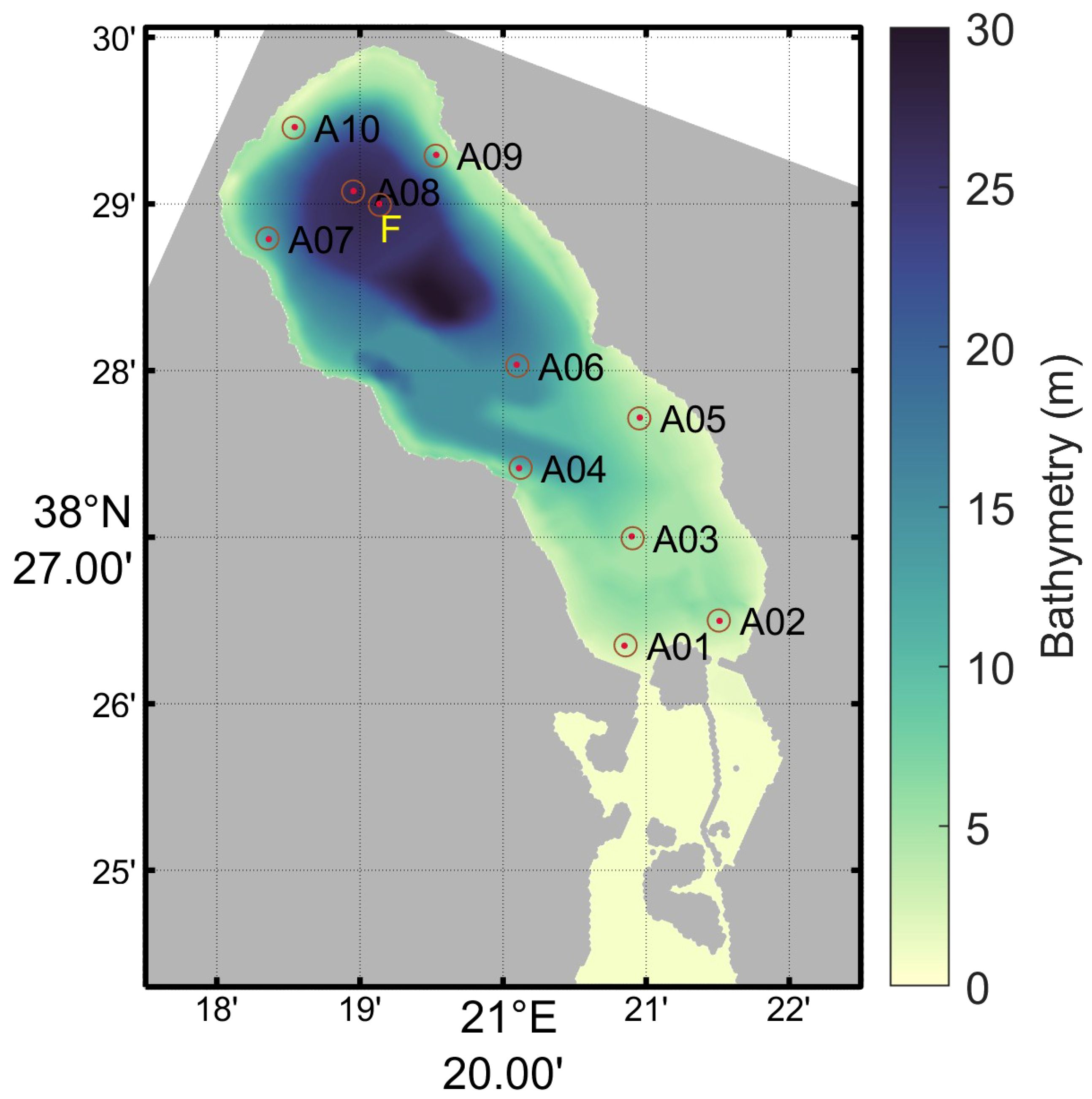
Figure 1 Points of the two measurement campaigns (A01–10: Campaign No. 1, F: Campaign No. 2).
During the period of 2013–2014, physicochemical data was gathered. A total of six cruises were conducted over eleven months, from July 2013 to May 2014. These cruises covered ten sampling locations within the Aitoliko Lagoon, with each station being visited at two-month intervals; see Figure 1. Water quality physicochemical variables, including temperature, pH, oxidation-reduction potential (ORP), dissolved oxygen (DO), and salinity, were monitored at each of the ten stations using a multi-parameter unit (Level TROLL 9500, In-Situ Inc.) at a depth interval of 0.5 meters.
In 2023, an environmental monitoring platform has been deployed in Aitoliko lagoon, in the framework of BLUE-GREENWAY project (Zacharias et al., 2023). One of the partners, Fugro (https://www.fugro.com/) has developed the platform based on one of Fugro’s standard floating monitoring platforms, the SeaWatch (SW) Midi185. This platform is powered by solar panels charging batteries during the day and using power from the batteries during the night. The system is also equipped with Iridium satellite communication transmitting the data in real time to Fugro Norway office in Trondheim, from where it is distributed to the BLUE-GREENWAY project partners.
The platform is equipped with a tripod mast with sensors for monitoring wind speed and direction, air temperature and humidity, air pressure. In addition the voltage measurements from the solar panels indicate the solar radiation. Under the buoy, as a part of the upper part of the buoy mooring, there is an inductive string with sensor placed at 2, 7 and 12 m depth. These sensors are monitoring water temperature, conductivity, pressure and dissolved oxygen.
The platform was installed and set in operation on February 2023 at 38.4832039°N latitude and 21.3189926°E longitude (point F in Figure 1).
For the needs of the present study, the 3D ocean model SINMOD was configured for the region. The physical, chemical and biological modules of SINMOD are fully coupled, and the model is run in a nested setup, as it is described further below. A comprehensive description of the physical, sea ice, chemical and food web components of the model can be found in Slagstad and McClimans (2005) and Wassmann et al. (2006).
SINMOD is forced by the following input: wind, heat exchange, evaporation, precipitation, tides and freshwater run-off from land. In addition, initial values of temperature and salinity for the boundaries are taken from the World Ocean Atlas (Boyer et al., 2018). The atmospheric forcing comes from the European Center for Medium-Range Weather Forecasts (ECMWF) ERA5 reanalysis database (Hersbach et al., 2020).
River discharge data were taken from the Swedish Meteorological and Hydrological Institute’s hydrological model “E HYPE” pan-European simulation results (http://www.smhi.se). Available data from this model contains daily run-off from 1980 to 2010. After 2010, we use the annual run-off average. The run-off data include nutrient (nitrogen, phosphorus and silicate).
According to Sannino et al. (2015), the inclusion of explicit tidal forcing in an eddy resolving Mediterranean model has non-negligible effects on the simulated circulation, in addition to the expected intensification of local mixing processes. Hence, eight tidal components were specified (elevation and currents) at the open boundaries of the Ionian model setup using data from the TPXO model of global ocean tides (https://www.tpxo.net/global), Knutsen et al. (2021). The tidal signal then propagates into the smaller model domains through the open boundaries.
SINMOD was configured in a multiple nested setup with an outer grid of 20 km resolution for the North Atlantic, a 4 km grid for the Mediterranean Sea, 800 m for the Ionian Sea, 160 m for the Gulf of Patras, and finally 32 m for the area of Messolonghi and Aitoliko lagoons in Greece; see Figure 2. The map projection used in this model set-up is Lambert’s conformal conic projection. The standard parallels are 30° and 60°N. Central meridian is 10°W. Bathymetry data for the models is Etopo1 (https://sos.noaa.gov/datasets/etopo1-topography-and-bathymetry/) which is a 1 arc-minute global relief model of Earth’s surface.
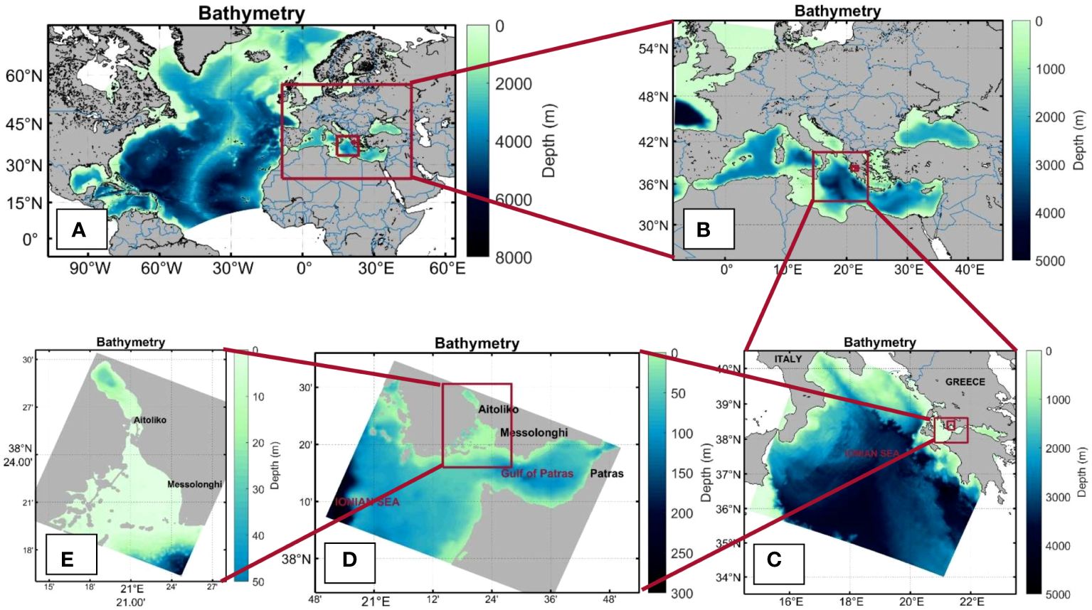
Figure 2 Computational domains of the nested numerical grids. (A): North Atlantic Ocean (20 km), (B) Mediterranean Sea (4 km), (C) Ionian Sea (800 m), (D) Gulf of Patras (160 m), and (E) Aitoliko-Messolonghi lagoons (32 m).
For the grid of the Ionian Sea (800 m) the model uses a z-coordinate in the vertical with a free surface and with a vertical level thickness of 2 m in the upper 10 m, 2.5 m down to 20 m, 5 down to 50 m increasing to 500 m below 2000 m; see, e.g., Figure 2C.
The 160 m model domain is embedded in the 800 m model. Elevation, u- and v-velocity are updated every 6 minutes, temperature and salinity are updated every 6 hours and atmospheric forcing is updated every 3 hours. The 32 m model has similar update intervals for the physical forcing coming from the 160 m model. The bathymetry of the 160 m and the 32 m model domains are shown in Figures 2D, E, respectively. The sources of input data for physical forcing of the finer model domains are the same as for the coarser models, just adapted to the new domains. The vertical coordinate system for the sub-kilometer scale models is z∗ instead of the regular z-coordinates in the coarser model domains. This means that the surface elevation is not only added to the surface layer, but is distributed over all the vertical layers. Hence the vertical layers are not longer strictly horizontal, but contains a small deviation. The z∗ coordinate system enables the use of very high resolution close to the surface, as we have used for the 32m model, see Supplementary Table S1 for an overview of the vertical levels for the 800 m, 160 m and 32 m models. Note that the vertical resolution of the 32 m model goes down to 75 m, although the maximum depth of the lagoon is ~30 m, because the model domain extends further southwards into the Gulf of Patras (Figure 2D), where the depth is greater than 30 m. This has been decided so that it could be obtained high resolution for both Aitoliko and Messolonghi lagoons with regards to exchange of water.
The 32 m setup of SINMOD model starts with specified profiles for temperature and salinity based on observations (Avramidis et al., 2015) and boundary conditions from the 160 m grid for the Gulf of Patras. The freshwater input is the same for all the simulated years, due to lack of available observations. In total 5 fresh water sources was used for the whole 32 m model domain (Figure 3) with a combined average volume flux adjusted to 3.9 m3/s. We found that we needed a little extra freshwater inside Aitoliko to maintain and, at times, reduce the surface salinity; so we added a diffuse runoff over the western part of Aitoliko. This is simply a small amount (here 0.02 m3/s) of fresh water added to the surface in specified grid cells in contact with land, summing up to 1.3 m3/s. The decrease in temperature and salinity towards the western side of the basin is a nonphysical consequence of the need to balance the salinity with the constant mixing with saltier water from south through tides. The diffuse runoff is continuously 1.3 m3/s while the pumping station was set to 1 m3/s average with a seasonal cycle applied.
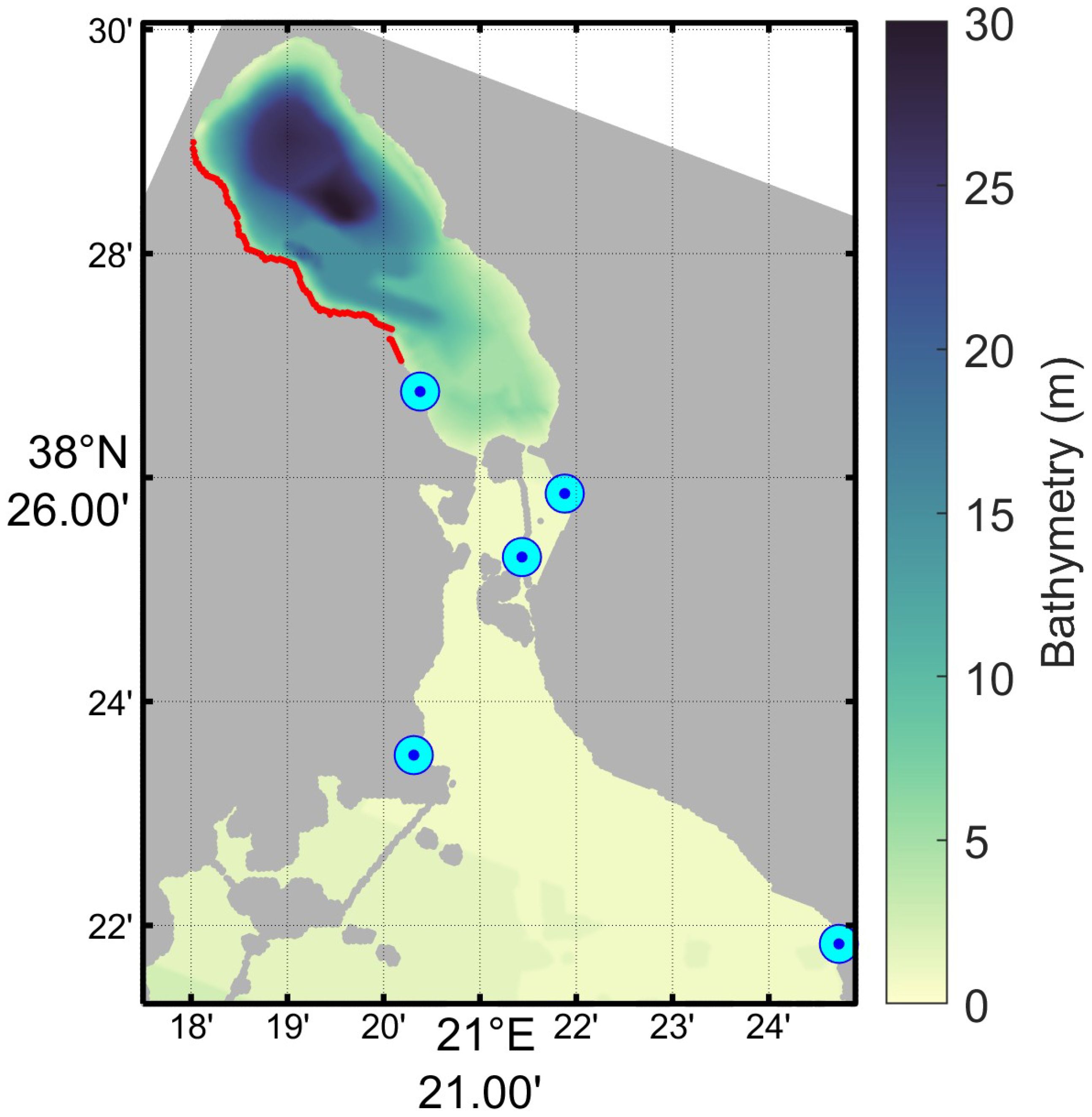
Figure 3 Points of fresh water influx (cyan) and diffuse (red). From north to south the mean flux was set to 1, 0.016, 0.016, 1.9 and 1 m3/s for the five points. The northernmost (cyan) point is the pumping station for the irrigation network. The sum of the red points was 1.3 m3/s.
The 20 km model was run for 12 years, producing boundary conditions to the 4 km model, which then was run from 2009 to 2020. See Figure 2 for overview of the model domains used. Initial field for the 20 km model was from World Ocean Atlas, and for the 4 km model we used a previous simulation, and for the 800 m model we used an interpolated field from the 4 km model. Temperature, salinity, current in x and y-direction was saved every hour for 38 vertical layers down to 3000 m depth (see also Supplementary Table S1), and surface elevation and surface wind was also saved. The higher resolution models were run for at least 10 years. The 800 m model for Ionian Sea (Figure 2C) was run 1.1.2010–31.12.2020 (Knutsen et al., 2021), the 160 m model domain of Patras Bay (Figure 2D) was run 1.1.2011–31.12.2020, and finally the 32 m model of the Aitoliko lagoon (Figure 2E) was run 1.1.2011–31.12.2020.
Initial fields for the smaller models were based on interpolations from the model which produced its boundary conditions. The 160 m model was run in 5 parallel simulations, each covering two years. The 32 m model was run in parallel jobs to save time, each simulation spanning two to three months.
The biological model is a modified version of an ecosystem model used for the Norwegian waters. The model is nitrogen based using the Redfield ratio for calculating Carbon and Phosphorus content in the biological components. The biological model (Wassmann et al., 2006) has 13 state variables: nitrate, ammonium, silicate, phosphate, diatoms, flagellates, microzooplankton (ciliates), small copepods, slow and fast sinking detritus, the microbial loop includes states for Dissolved Organic Carbon (DOC), bacteria and heterotrophic nanoflagllates. Oxygen concentration is calculated from production by the algae and respiration and degradation of living and dead organic material and exchange with the atmosphere. SINMOD includes a state for PO4, but this does not include processes in anoxic layer, such as release of PO4 from the benthic layer. In addition, there were very little information about release of PO4 from the rivers. We have thus not included PO4 in the current study, even though it can be limiting phytoplankton growth during winter (Gianni and Zacharias, 2019).
For the 160 m setup, the biological model was initialized by input data from the following Copernicus Marine Service (CMEMS) product GLOBAL_REANALYSIS_BIO_001_029, which contains 3D monthly mean fields of chlorophyll, nitrate, phosphate, silicate, dissolved oxygen concentration.
The hydrodynamic model takes its initial- and boundary conditions from the model of the Ionian Sea. The biological model uses zero gradient at the boundaries, which means that the value of biological variables close to the boundaries are extrapolated out to the boundaries and that the boundaries do not contribute to the internal domain of the 160m model. Light attenuation is a sum of physical properties (e.g. turbidity) and biological biomass (Chlorophyll). The biological attenuation comes from the model, but the physical part need to be specified. According to Gianni et al. (2012), we specified a Secchi depth of 3 m in the Messolonghi lagoon caused by turbidity alone and 8 m in deeper water. Using Kirk’s formula, the light attenuation coefficient is Kd=1.4/Secchi Depth (Kirk, 1994).
For the 32 m setup, the initial field of biological variables were interpolated from the 160 m. To save computer time, a new start field was interpolated for the start of each of the 32 m model runs. Inside the Aitoliko basin the vertical temperature, salinity and oxygen profiles were modified to resemble observations in Avramidis et al. (2015), and relaxation (nudging a variable towards predefined values, here the initial field) of temperature and salinity at depth was used to help preserving the observed vertical gradient in salinity. The hydrodynamic and the biological modules take their boundary conditions from the 160 m model though a nesting technique.
The analysis procedure followed is presented in detail in Stefanakos (2021). Here only a brief account is given, according to which both the physical (current speed, temperature, salinity, wind speed etc) and the biological (oxygen, chlorophyll etc) parameters are modeled either as 2D or 3D fields of the form
where i runs over the time, j over the latitudes ϕ, k over the longitudes λ, and ℓ over the depths z, respectively.
Then, the statistical analysis of fields Equations (1) and (2) is benefited by introducing Buys-Ballot triple time index (y, m, n) (Stefanakos et al., 2006) in order to properly treat variability at different time scales. The first component y is the yearly index and runs over the number of years Y, m={1,2,…,12} is the monthly index, and n={1,2,…,Nm} represents the time within a month, with Nm be the number of α-hourly observations within the m-th month.
Especially, the following quantities depict the seasonal variability of the data, and they have been used in a nonstationary modeling suitable for metocean and maritime parameters; see Athanassoulis and Stefanakos (1995); Stefanakos et al. (2006); Stefanakos and SChinas (2014):
Mean Monthly Variability (MMV)
Mean Annual Variability (MAV)
where μ32 (y,·,·,·), σ32 (y,·,·,·) and Ny are defined in the following Equations (5)–(7), respectively.
Inter-Annual Variability (IAV)
where (·,·,·) is defined in the following Equation (9).
The vertical profiles of observed dissolved oxygen reveal permanent anoxic conditions below a depth ranging from 7 to 13 m, depending the seasonal and spatial distribution. The dissolved oxygen concentration in the deeper points (A06–10) ranges from 7 to 12 mg/L in the surface and presents a strong oxycline from 5 m to 15 m depth. The oxycline is deeper from September to March, and shallower from May to July. In September, there also seem to be more oxygen rich water mixed down to 20 m at A09; see Figure 4. Note, e.g., that, at point A08, anoxic conditions starts at about 7 m depth in September, while in January they start at about 13 m depth.
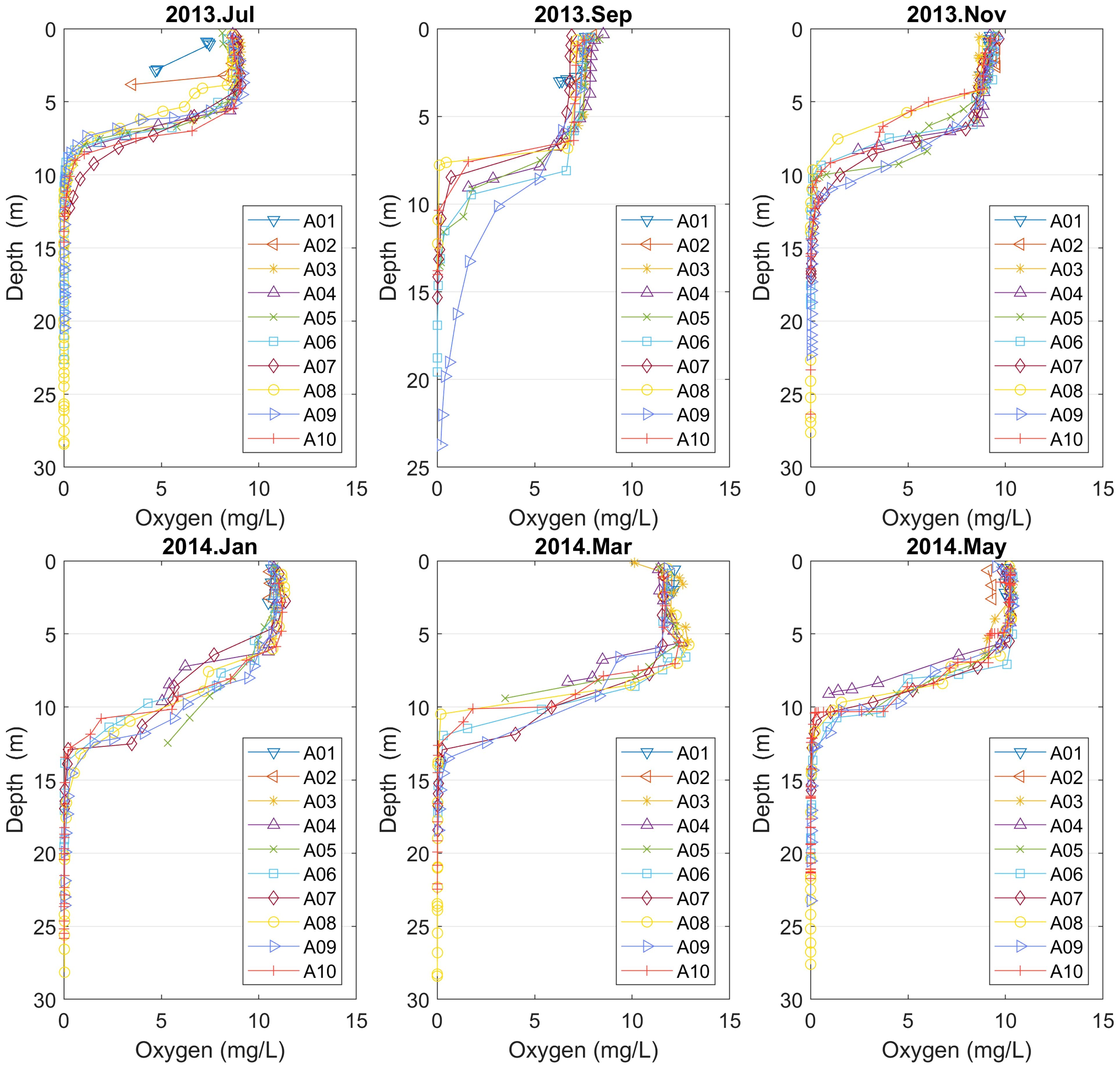
Figure 4 Vertical oxygen profiles for points A01–10 (Campaign No. 1). Note that in September anoxic conditions starts at about 7 m depth at point A08, while in January anoxic conditions start at about 13 m depth.
Concerning salinity profiles, a characteristic halocline zone is found ranging from 6 m to 15 m depth with values from 17 to 23 ppt. In addition, the spring’s vertical profiles are similar in the different parts of the Aitoliko basin, with salinity values beginning from 15 ppt at the surface and rise to around 25 ppt in the deeper parts. In contrast, November’s salinity vertical profiles spread between 19–25 ppt for the deeper points; see Figure 5. In July (A02 and A03) and September (A01 and A03) there are two shallow stations that have a higher salinity close to the bottom. This can be saltier water coming in from the south and flowing below the fresher water of Aitoliko. In July at A03, there is a corresponding temperature signal, which cancels the signal in density. This mechanism of inflow is expected to be responsible for the seasonal fluctuations in salinity at depth in the Aitoliko lagoon.
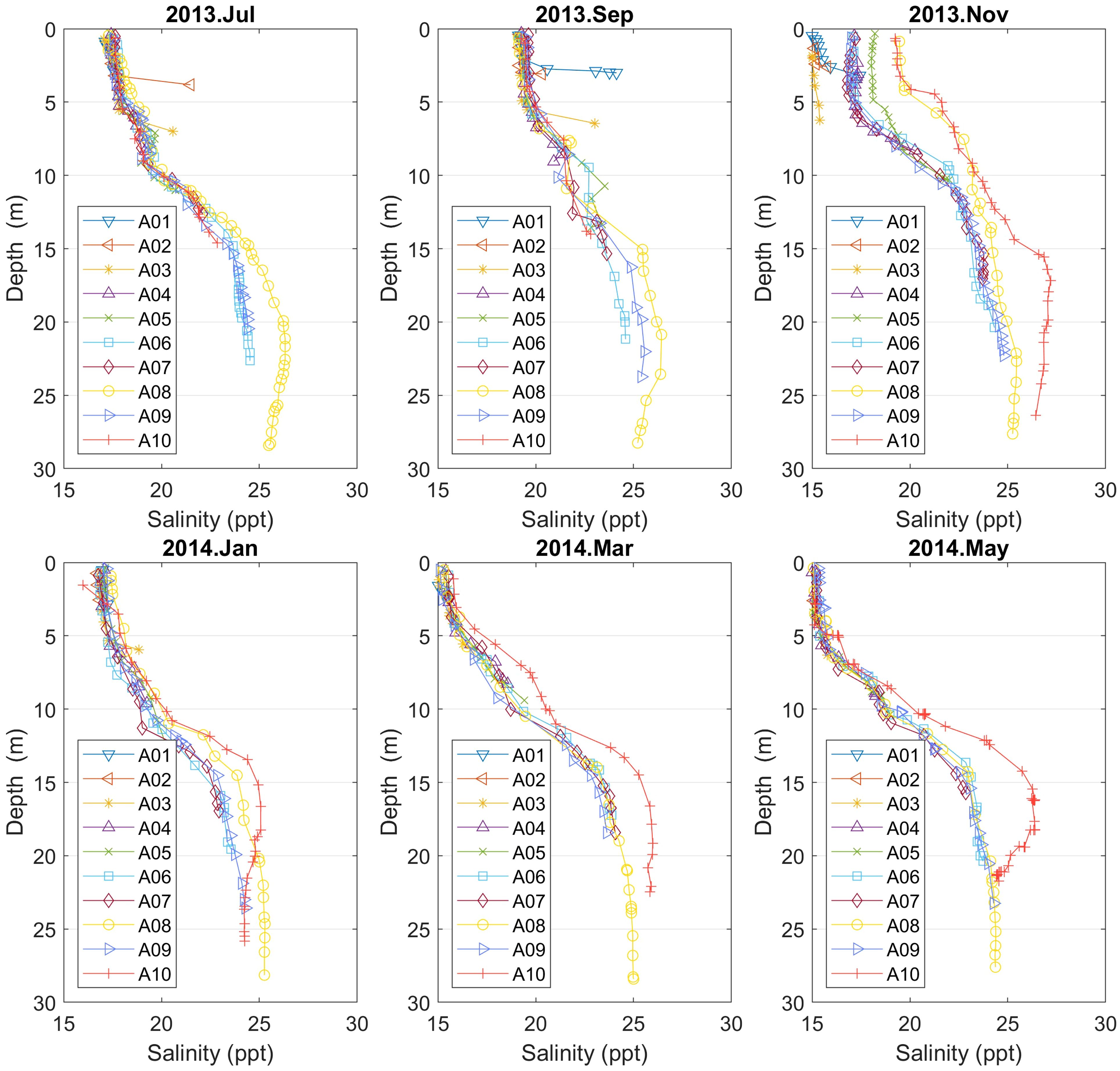
Figure 5 Vertical salinity profiles for points A01–10 (Campaign No. 1). From November to May A10 has the highest salinity for most of the water column, suggesting that there is little freshwater supply in the northern end of Aitoliko. In November, A01–03 are fresher than the other stations, which might be related to freshwater from the pumping station.
The highest salinity values at all depths from November to May is observed at point A10. This fact indicates that there is little freshwater supply in the northern end of Aitoliko in this period (November 2013-May 2014). Another possible explanation could be that upwelling occurs in north between September and November, explaining the higher salinity for A08 and A10 for the whole water column in November and the corresponding lowest oxygen values in the oxycline. The vertical density profiles (Figure 6) of A08 and A10 support this hypothesis and there is also a reduction in salinity below 15 m depth from September to November 2013 at A08. The wind direction was variable during November 2013, but it did come continuously from north for about one week.

Figure 6 Vertical density profiles for points A01–10 (Campaign No. 1). The profiles are quite similar to the salinity profiles.
From November to January there is mixing in Aitoliko, significantly reducing the horizontal differences in salinity in the upper 15 m. Below this, there is a freshening of most of the profiles except A08 below 20 m depth (which is near 25 ppt from November to March). From September to May there is a freshening of most stations in the upper 5 m (from about 19 to 15 ppt) which must come from freshwater runoff as the salinity below and outside Aitoliko is higher. Also, during November 2013, points A01–03 are fresher than the other stations, which might be related to freshwater from the pumping station.
Furthermore, the study of vertical temperature profiles displays a thermocline zone between 5 to 15 m depth located central and central north of the Lagoon. Temperature values vary between 13 and 28°C with sharper thermocline which goes deeper during July and September; see Figure 7. All in all, one can see that there is little spatial variation, but significant vertical and seasonal variation in temperature.
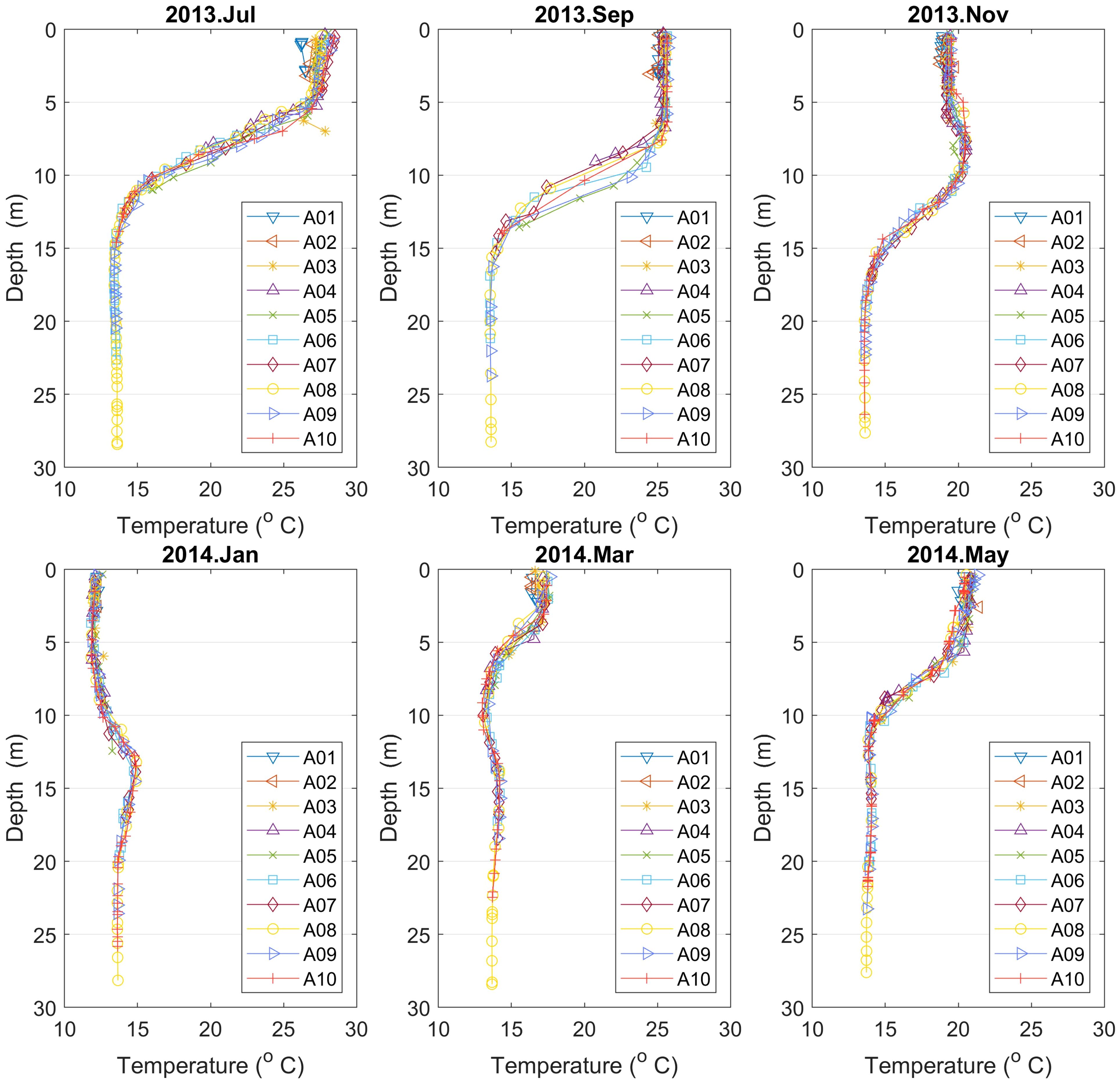
Figure 7 Vertical temperature profiles for points A01–10 (Campaign No. 1). There is little spatial variation, but significant vertical and seasonal variation in temperature.
In the following, after combining temperature and salinity to estimate the density, one finds that vertical density profiles are quite similar to the ones of salinity; see Figure 6. Thus, there is a strong pycnocline zone from 5 m to 15 m for the deeper points (A06–10). Aitoliko Lagoon’s density values span from 1010 to 1020 kg/m3.
The sampling stations located nearer to Messolonghi lagoon (A01–03) are very shallow, and, thus, are affected by the low renewal of waters through the small bridges with Messolonghi lagoon. Therefore, they present almost constant profiles for all variables.
In summary, the spatial differences of salinity between sampling stations are equally pronounced than their seasonal variability. Other factors, such as temperature and density, also present this spatial variability. The minimum water renewal from Messolonghi lagoon strongly affects the spatial variation of these variables. This analysis underscores that the hydrodynamics of Aitoliko lagoon depend both as a function of season and space.
In Figure 8, vertical profiles of oxygen, salinity, temperature, and density are plotted based on measurements from the floating platform at point F; see Figure 1.
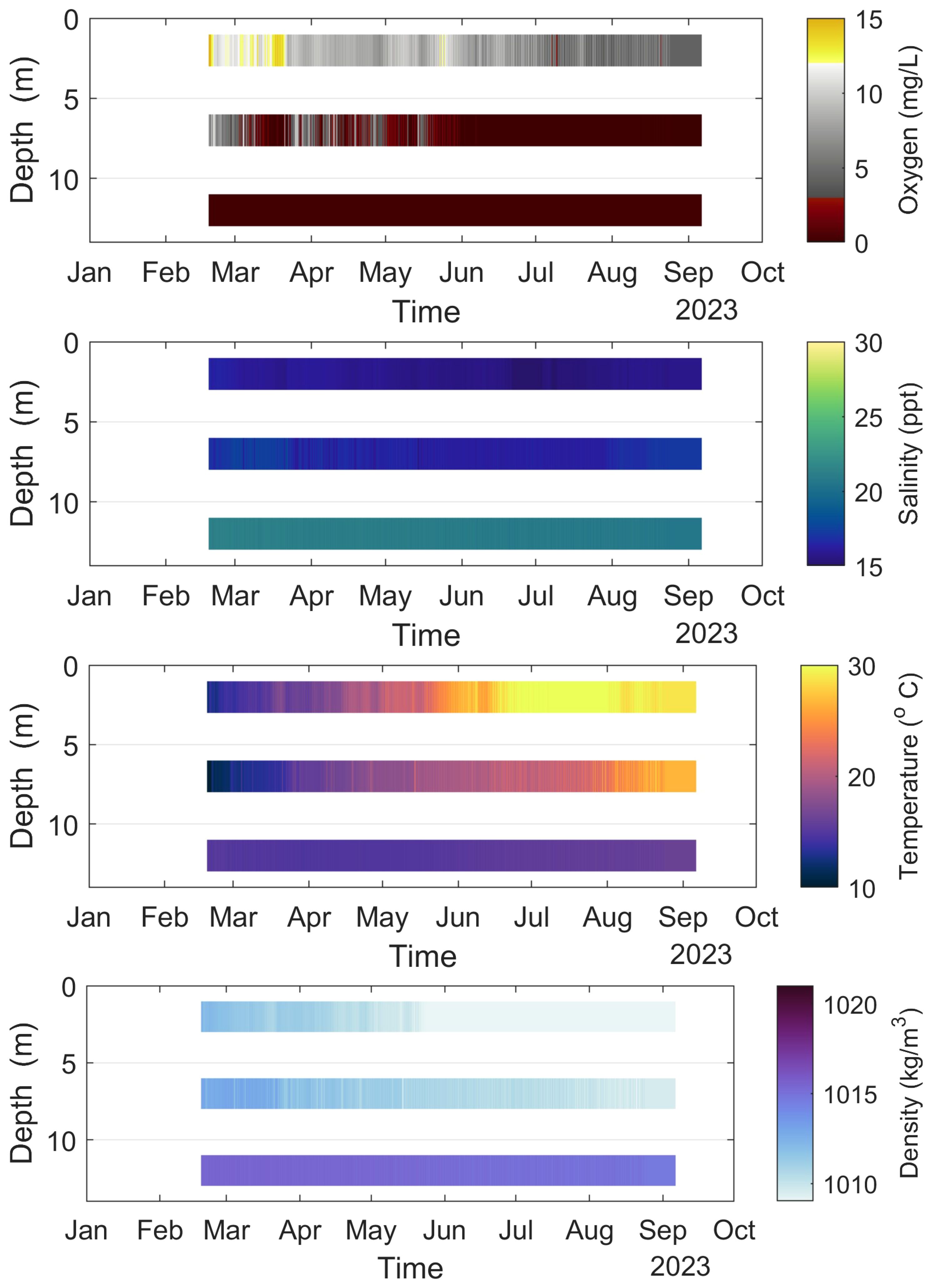
Figure 8 Vertical profiles of oxygen, salinity, temperature, and density for point F (Campaign No. 2).
The vertical profile of oxygen is constantly anoxic from February to August 2023 under 12 m depth. On the 2nd of June, it was recorded that anoxia raised at 7 m depth, and, during the whole summer season, the anoxic layer was reached between 7 to 2 meters depth. Comparing the present (2023) field measurements with earlier published observations (Gianni et al., 2011, 2012; Chamalaki et al., 2014; Avramidis et al., 2015), the anoxic layer is well above 5 m depth. It is expected that the anoxic conditions below 7 m depth will continue until the first autumn winds, which will force upper layer water circulation, and the anoxia will again be found only below 7 m (Gianni and Zacharias, 2015).
The vertical salinity profile presents a halocline zone from February to August 2023 with salinity values spanning between 15–22 ppt. The time period between the 27th of June and the 9th of July, a constant salinity decline is remarked at 2 m depth. The salinity at 12 m depth has been almost constant around 21 ppt, while the salinity at 2 m has been 15–16 ppt, and 16–18 ppt at 7 m depth. It is observed a steep decline and a steep rise of salinity for this period, which cannot be considered as a result of a meteorological or water hydrodynamic change. It is rather explained as a result of large input of non-saline water, most probably from Lysimachia lake.
Further, the results of the first half of the year show that the air temperature rose from 10–15°C in the spring till 30–35°C in the last part of the summer. The water temperature at 12 m depth increased from 15 to 16°C in this period, while the temperature at 2 m depth has almost followed the air temperature.
The Aitoliko lagoon (max depth 28 m) is connected to the ocean only through the shallow Messolonghi lagoon (depth 1–2 m). This naturally prevents the exchange of bottom water from Aitoliko with the Patras Bay. In addition, extra nutrients from the surrounding farmed land that uses chemical fertilizers (Zacharias, Personal communication, 2023) come into the lagoon mainly through the pumping system for the irrigation network. The wind speed in the area is mostly moderate. For 2019, the ERA5 data showed less than 6 m/s wind speed in 96% of the time and less than 8 m/s 99.5% of the time. Max wind speed for 2019 was 11.6 m/s in February, and mean was 2.5 m/s.
Online tidal charts for Aitoliko show typically semi-diurnal tides with tidal amplitude of 0.1 - 0.2 m (https://www.tidetime.org/europe/greece/aitoliko.htm). The model reproduces this pattern, but with slightly reduced amplitude (not shown).
To ensure that we are able to reproduce the hypoxia/anoxia conditions in the lagoon, we have examined and modified several numerical routines in the model with regard to vertical stability in the water column and develop the model to be more appropriate for ultra-high resolution for a lagoon as Aitoliko. In addition, we used relaxation of temperature and salinity in the hypoxic/anoxic part of the basin and paid extra attention of the density profile used as initial field in Aitoliko for all simulations. The model was then run for 10 years in 2–3 months periods on our HPC system as multiple parallel jobs.
Although results of all three last grids (800 m, 160 m and 32 m) are available, we will focus on the description of the results for the higher resolution area (32 m); see Figure 2E. The interested reader can also find the results for the Ionian Sea (800 m) in Knutsen et al. (2021).
The most important driving forces for the dynamics in the Aitoliko lagoon are the tides coming in from the south, freshwater supply and wind forcing. All those drivers may not be important during all seasons, and we expect the effect of tides to be a bit underestimated as the tidal difference was generally just below 0.1 m while the online charts show 0.1–0.2 m. When we plot annual average maps of currents, we find that the inflowing tides seem to bend towards the east (right) and flow northwards. The freshwater supply we have applied tend to disperse out near the surface, towards the interior of the basin and bend southwards back towards the Aitoliko Island. This becomes a cyclonic circulation on average, and this pattern is more pronounced in the southern and shallow part of the lagoon than in the northern, deeper part where we occasionally also see anticyclonic circulation. The current speeds are generally weak at a few cm/s. The strongest currents are in the passages besides the Aitoliko Island where the model presents 9 cm/s average surface currents. Monthly averages could be 2–3 times stronger. At times the inflowing tides forma cyclonic eddy near south west part of the Aitoliko lagoon, and this can in part work together with the freshwater supply from the pump station feeding the western part of the eddy. When this happens the cyclonic circulation in the lagoon is weaker as it then is not continuously driven from the inflowing tides. At 10 m depth we see mainly a weak anticyclonic circulation in the deeper part of the lagoon with monthly mean speed up to 1 cm/s.
The Mean Monthly Variability (MMV) of surface currents is calculated on the basis of Equation (3) and it was found small. The monthly mean values are less than 2 cm/s in most part of the lagoon, with larger values in the western/southwestern area. The surface currents are larger, reaching 10 cm/s near the bridge on Aitoliko Island; see Supplementary Figure S1. The monthly mean values of temperature, salinity, oxygen and chlorophyll are spatially homogeneous.
Furthermore, the deviation between the cooler months (11–15°C) and the warmer ones (26–32°C) is greater than in the open sea due to the limited exchange with the open sea and, therefore, increased importance of air-sea interaction. The monthly mean surface oxygen exhibits higher values during January-May (7.5–9.5 mg/L) and lower during July-October (6.5–7.5 mg/L), whereas the mean values are presented on Supplementary Figures S2, S7, S15, S21. The MMV of wind speed follows the usual seasonal cycle with higher values during the winter months (January-February, November-December), whereas wind direction changes from SW (January-March) to NW (April-September) and, then, E-SE (October-December); see Supplementary Figure S12.
In addition, and in order to investigate MMV along depth, a cross-section is considered, crossing the deepest point of the lagoon and extending a bit further out to the Messolonghi lagoon; see embedded map in Figure 9. The section’s length is approximately 8 km, and the deepest point is a bit less than 30 m. Current speed is layered horizontally in this cross-section, with generally low values. The highest values are being in the surface and in a layer at an average depth of 10 m (7–15 m). This layer is deeper (15–20 m) from May to October. In the surface, water is on average moving southwards (out). There is a compensating flow near 7 m depth in Jan-April (in the northern end of the section), whereas a quieter layer is found between this level and the surface. The compensating flow changes throughout the year, deepening in summer/fall in the model; see Figures 9.
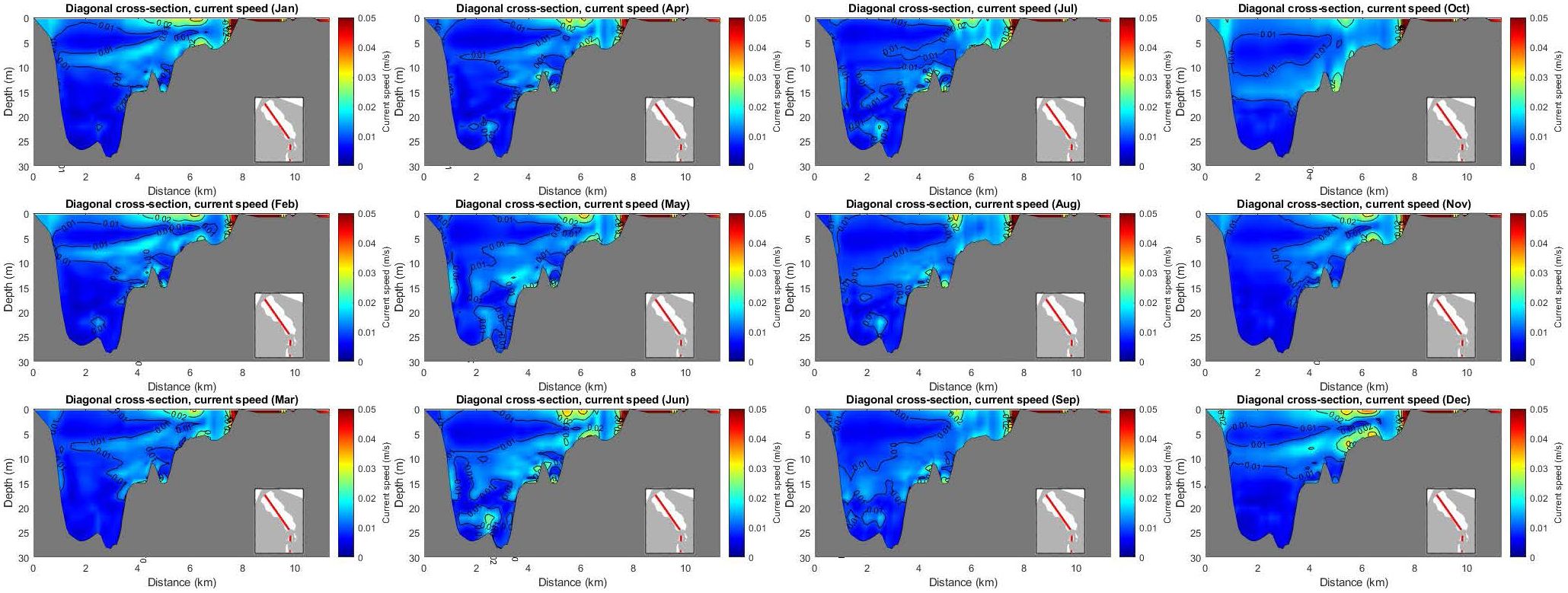
Figure 9 Mean monthly values of current speed in a cross-section.
The temperature in this cross-section is layered horizontally in the deeper parts, while there is a spatial stratification in the shallower areas. Note also that the water at the deeper parts is warmer than the surface during the colder months (January-February, November-December); see Supplementary Figure S6, On the other hand, salinity is well layered horizontally with a layer of high salinity in the bottom of the lagoon during all months; see Supplementary Figure S11. Oxygen shows similar layered behavior like salinity. That is, lower oxygen concentration in the deeper part of the lagoon, with the hypoxic layer going up during the warmer months, in Figure 10.
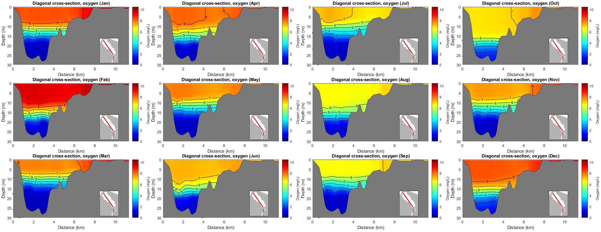
Figure 10 Mean monthly values of oxygen in a cross-section.
We will now present the Mean Annual Variability (MAV), and the Inter-Annual Variability (IAV) defined in Equations 4, 8. MAV of surface currents and wind speed show considerably high values (80% and 62% of the mean value, respectively), which means that there is no significant seasonal variability. Currents has highest values in the deeper part of the lagoon and near the island. Then, surface temperature and chlorophyll exhibits medium variability (32% and 30% of the mean value, respectively). On the other hand, salinity and oxygen show lower values (1.7% and 7.5% of the mean value, respectively), i.e. there is significant variability within the year especially in the upper layer (0–5 m).
Concerning IAV, all parameters (except chlorophyll) exhibit lower values than in MAV (currents: 8% of the mean value, temperature: 1.5%, salinity: 0.5%, oxygen: 1.5%, wind: 2.2%), which are more spread both in the deepest part and the coastal areas of the lagoon.
Examples of MAV and IAV for surface currents and temperature are given in Figure 11. Additional figures can be found in Supplementary Material; Supplementary Figures S8, S9, S13, S14, S16, 17, S22, S23.
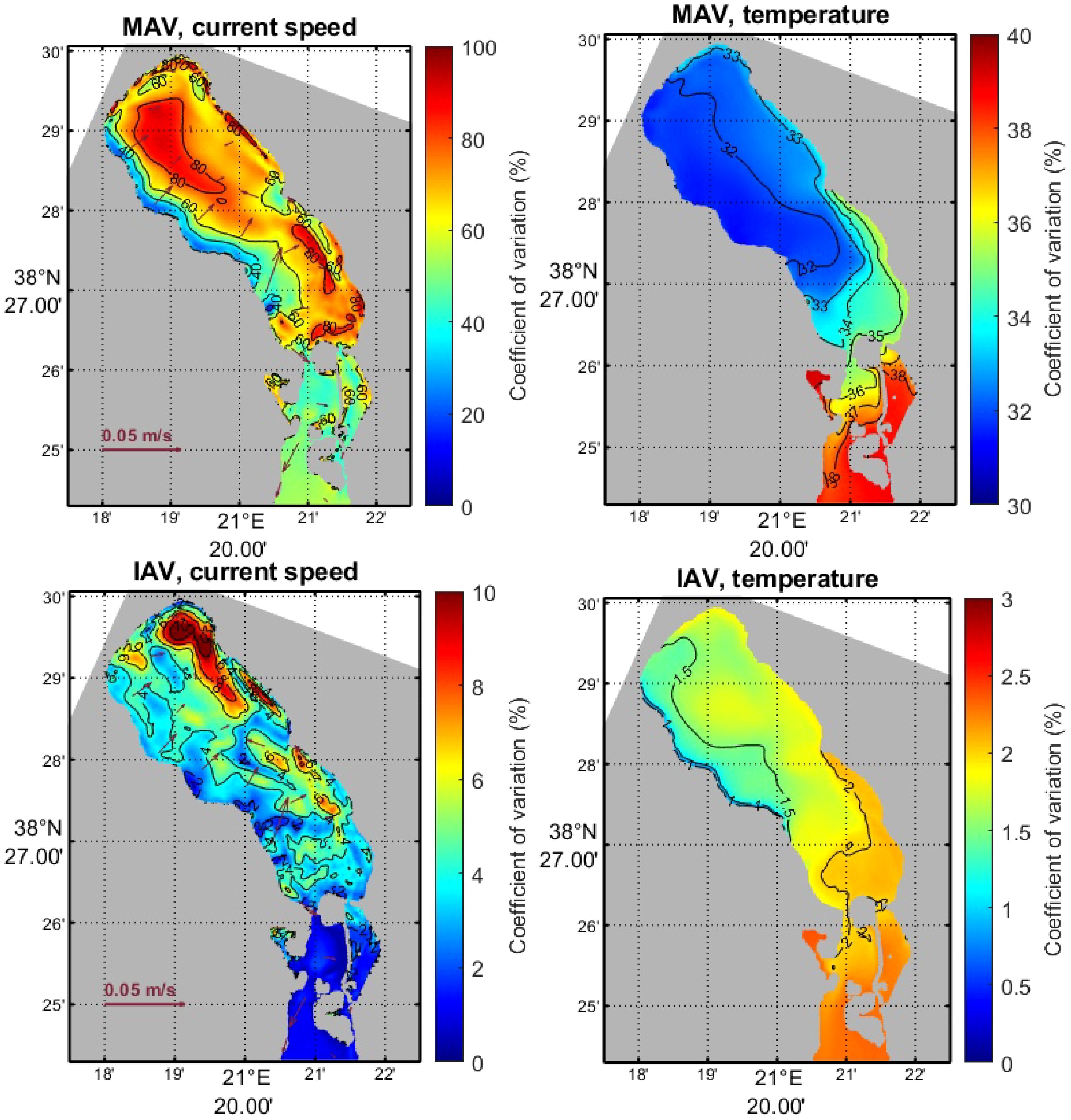
Figure 11 Mean Annual Variability (upper panel) and Inter-Annual Variability (lower panel) of surface currents and temperature.
In Figure 12, a condensed view of the modeled time series is shown for temperature, salinity, density, current speed, oxygen, Brunt-Väisala frequency and Richardson number for the deepest part of the lagoon (point F in Figure 1). The figure comprises monthly means for the vertical layers in Hov-Moeller diagrams as a first glance at seasonal and interannual variability. The ranges are clearly found for the different variables, outlining a seasonal cycle for the first three panels. Temperature exhibits a reasonable variability in the upper water column. However, the summer temperature (for one or two months per year) reaches to the bottom, which is not supported by the measurements; see Section 3.3. Salinity appears to be more in line with observations with a sharp halocline from nearly 10 m to 20 m depth. As the density is determined by temperature and salinity (we disregard pressure at the depths of Aitoliko), the too deep summer mixing of temperature weakens the vertical density gradient and hence vertical mixing can be too strong.
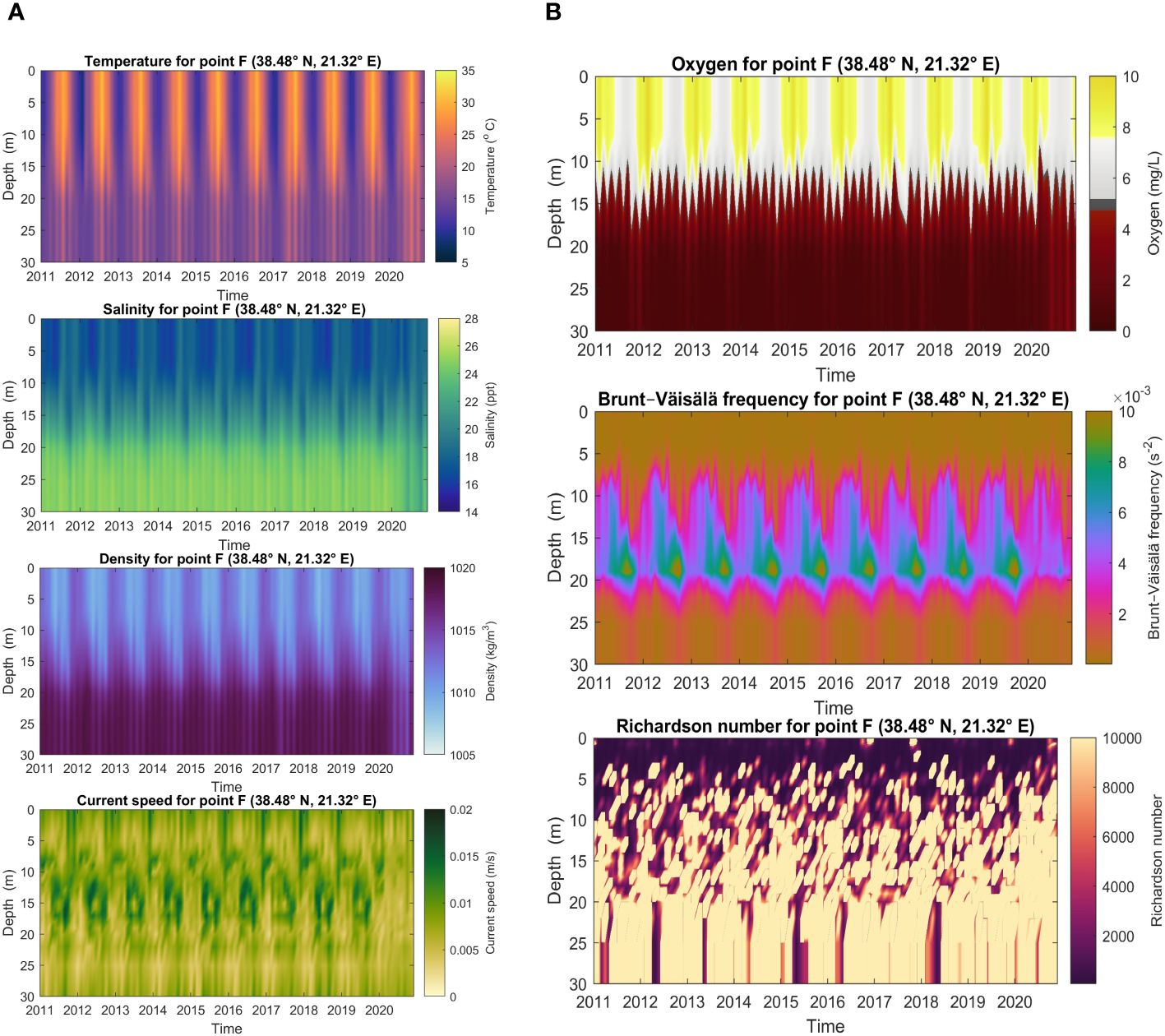
Figure 12 Hov-Moeller diagrams for the gridpoint closest to point F. (A) Temperature, Salinity, Density, Current Speed, (B) Oxygen, Brunt-Väisala frequency, Richardson number.
Current speed at the interior of Aitoliko shows a clear seasonality with strongest monthly means in the late autumn in the surface. Also, there are increased current speeds at intermediate depth, but generally not simultaneously as in the surface. This might be related to inflowing salty water that sinks beneath the very fresh surface water, but it is also possible that the relaxation method applied for temperature and salinity below 8 m depth leads to some non-physical features. The model shows small current speeds near the bottom, which is expected.
Oxygen shows a clear seasonal cycle in the upper water column, but not in the lower part in accordance with measurements. The euphotic zone in the model reaches too deep, as the newer measurements show, i.e., sometimes hypoxic at 7 m depth. The model compares better for the older oxygen measurements (Figure 13), although in summer the model estimates the hypoxic level 4–5 m too deep.
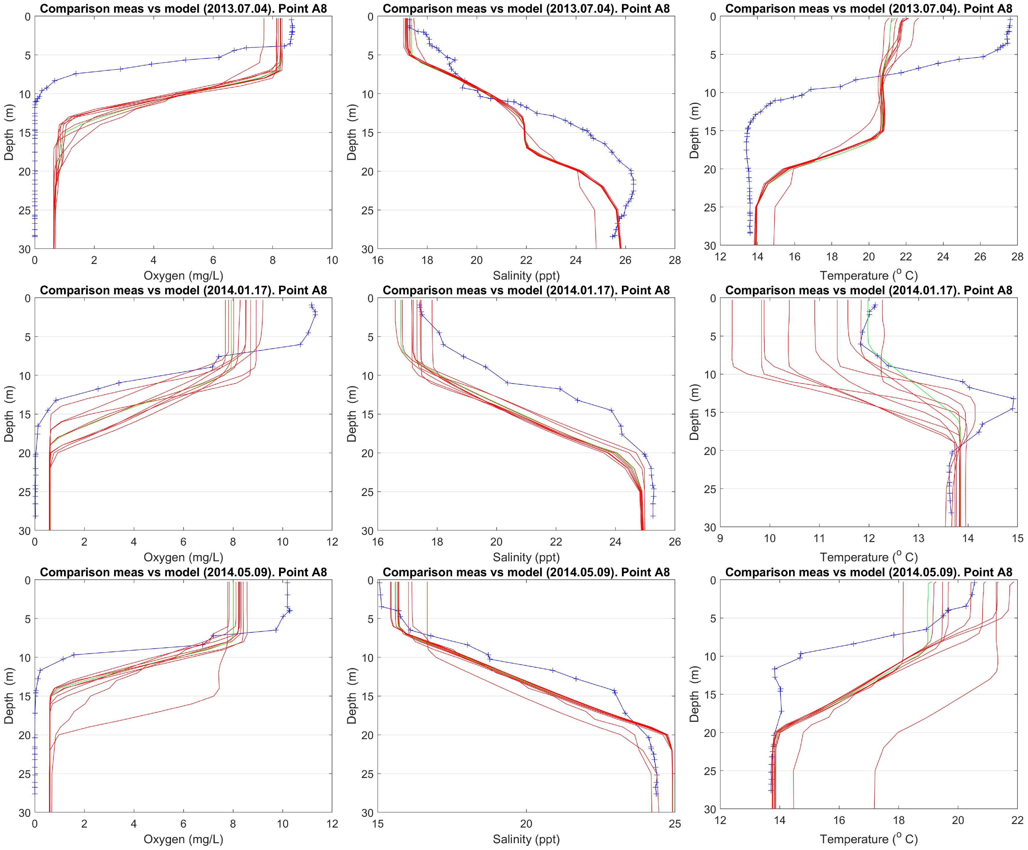
Figure 13 Comparison of model data vs Campaign No. 1 measurements.
The Brunt-Väisala frequency (BVf) is highest in the 15–20 m depth range, which is related to the temperature-salinity profiles that has strongest vertical gradient in that depth interval. Probably this should be shallower, again linked to too deep vertical mixing. Its seasonal cycle is clear and in the autumn the BVF increases towards the bottom. Low values near the surface indicate that well mixed upper ocean throughout the year.
The Richardson number in the last panel of Figure 12 indicates high stability as is expected both due to vertical gradients in temperature and salinity, but also due to low current speeds inside the lagoon.
In this section, model results are compared against measurements gathered in the two measuring campaigns described in Section 2.2.
For Campaign No. 1, there are 10 available measuring points at 6 distinct dates. For each one of these dates and points, model data have been retrieved for each one of the 10 years (2011–2020). In Figure 13, one can see vertical profiles of oxygen, salinity and temperature using model (red lines) and measured (blue line) data for three dates (2013.07, 2014.01, 2014.05). The model simulates a too deep hypoxia layer compared to the measurements. The model also underestimates oxygen concentrations in the surface layers. Salinity profiles show similar level of agreement, while temperature profiles exhibit higher discrepancies. Full account for the comparison of data for all dates can be found in Supplementary Figure S25.
The second comparison refers to Campaign No. 2 measurements, which were taken during Feb–Aug 2023. The measurements come from three specific depths (2, 7 and 12 meters) every 1 hour. So, for each depth, there is a statistically significant population to calculate the monthly histogram of the measured population; see the light blue zone in Figure 14. In addition, in the same figures, the 90% of the probability mass (between percentiles 5% and 95%) is marked as yellow zone, and the median as a cyan circle. Also the raw measurements are shown as crosses. Full account for the comparison of data for all dates can be found in Supplementary Figure S26.
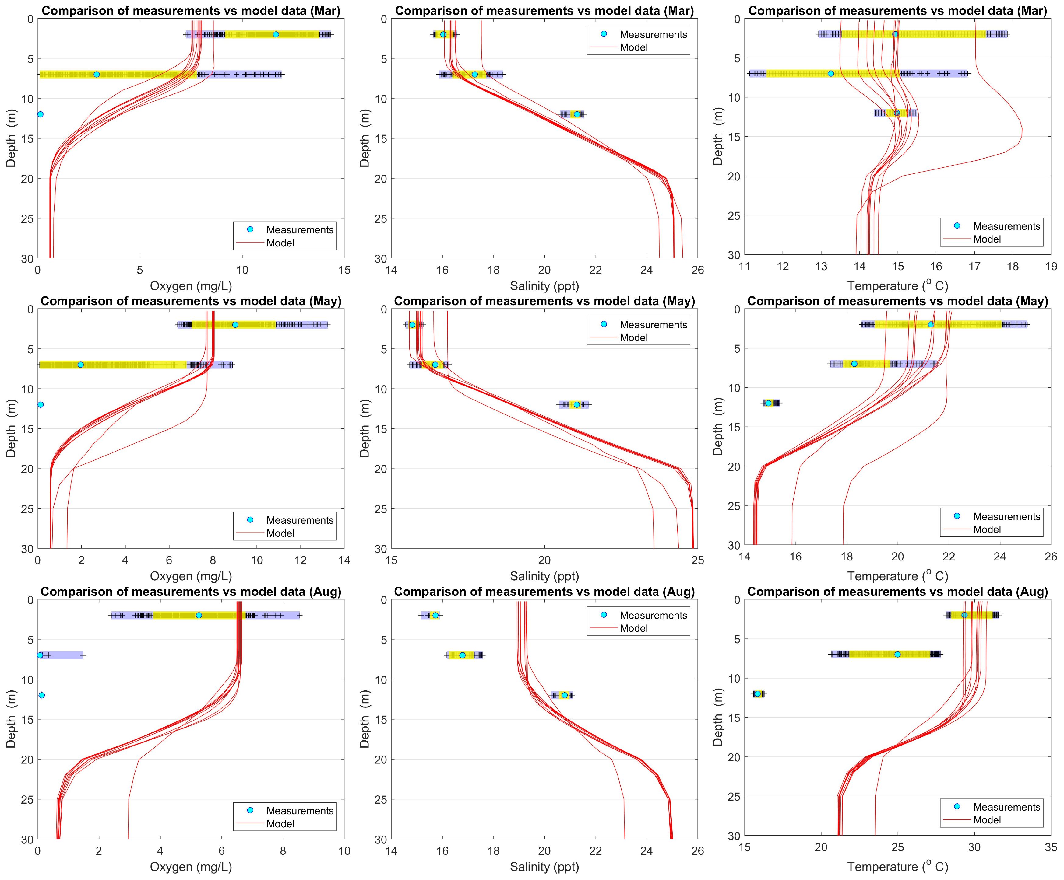
Figure 14 Comparison of model data vs Campaign No. 2 measurements.
In general, there are several discrepancies between model results and measurements, in particular in the deeper parts. On the other hand, there is partial agreement in some cases in the surface depth layers; see, e.g., temperature (March and May), salinity (March and May) and oxygen (August). In any case, it should be noted that the comparisons should be considered as a first “offhand” effort, since the nature of model and measured data differs. In the first case (2013–2014), the measurements originate just from a specific day/time. Even in the second case, measurements come from a specific year, which cannot be considered by any means representative or typical for the lagoon.
The objective of this research is to investigate the evolution of hypoxia/anoxia levels in Aitoliko lagoon, Greece. For this purpose, data from two measuring campaigns have been used along with results of the 3D ocean model SINMOD. The model has been calibrated and validated based on the field studies that have already been performed by our team; see, e.g., Papadas et al. (2009); Gianni et al (Gianni et al., 2011, 2012; Gianni et al., 2013); Gianni and Zacharias (Gianni and Zacharias, 2012, 2015); Kehayias et al. (2013); Chamalaki et al. (2014); Koutsodendris et al (Koutsodendris et al., 2015; Koutsodendris et al., 2017).
It should also be noted that the SINMOD biological module incorporates the influence of oxygen concentration through photosynthesis, respiration, and remineralization. It is configured to account for nutrient loads from land (nitrate). Additionally, the model integrates a basic connection to the benthic environment. We should, however, stress that the primary focus of the numerical modeling is to investigate how physical processes impacts oxygen distribution.
The analysis of results includes monthly, annual and interannual variability of fields of (i) current speed, (ii) temperature, (iii) salinity, (iv) wind speed, (v) oxygen, and (vi) chlorophyll. Some of these fields are at the sea surface (wind speed, chlorophyll), whereas others are both at sea surface and along a cross-section (current speed, temperature, salinity, oxygen).
The analysis of such a large amount of data (a decade) at a high spatial (32 m) and temporal (1 hour) resolution, gives us the opportunity to investigate the variability in seasonal (monthly, annual) and inter-annual scales.
Temperature exhibits reasonable variability in the upper water column, although summer temperature reaches in some cases the bottom, which is not supported by the measurements. Model salinity agrees better with observations with a sharp halocline from about 10 m to 20 m depth. As the density is determined by temperature and salinity, the too deep summer mixing of temperature weakens the vertical density gradient and hence vertical mixing can be too strong.
Current speed in the interior of Aitoliko shows a clear seasonality with strongest monthly means in the late autumn in the surface. Also, there are increased current speeds at intermediate depth, but generally not simultaneously as at the surface. This might be related to inflowing salty water that sinks beneath the very fresh surface water which is expected, but it is also possible that the relaxation method applied for temperature and salinity below 8 m depth has some non-physical features here. For example if the relaxation pulls the temperature or salinity towards the values of the initial field more on one side of the basin than the other, this will modify the horizontal pressure gradient and hence it can set up a current. In addition, the model shows low current speeds near the bottom, which is expected.
Finally, oxygen shows a clear seasonal cycle in the upper water column, but not in the lower part in accordance to the measurements. The euphotic zone in the model reaches too deep, as the measurements show hypoxic at 5–7 m depth, while the model gives estimates of the hypoxic level 4–5 m deeper.
Some possible causes for these partial discrepancies with the measurements could have been that the light penetrates too deep and heats up too much of the water column compared to what happens in the field. The secchi depth should probably be set to a lower value. Measured secchi depth in Aitoliko is on the order of 1 m (Zacharias, pers. comm.), which contributes to absorption of solar radiation in the surface layer and hence preventing heating below. This means that the surface water will warm up faster than in clearer water (and in the model), creating a vertical density gradient that reduces vertical mixing.
Another issue in this study is the accuracy of the freshwater budget. The database from SMHI does not cover the study period and we use long-term average instead, for all years. This is an obvious simplification that reduces the modeled variability. Future studies of the Aitoliko should strive to get high quality freshwater data for the region, in addition to measured time series of sea surface elevation for model calibration of water fluxes due to tides. Inaccuracies in freshwater supply will affect vertical stability and mixing, in addition to horizontal currents.
Comparison of the measured wind force and direction at the buoy in Aitoliko with the ERA5 dataset for the months of overlapping data, indicate that ERA5 is adequate for this study although the spatial resolution is low.
We experienced some noise in the velocity field that we managed to get rid of by manipulating the advection scheme. However, there might still be numerical noise that is not large enough to be clearly visible but still can affect, for example, vertical mixing. One could argue that we are pushing the limits for a hydrostatic model at 32 m horizontal resolution, and that a non-hydrostatic model should have been used for this application. That would be a fair criticism; however, we find it interesting to see what a regular hydrostatic model can do at ultra-high resolution. The problems with the model in this application are, as we see it, mainly related to vertical mixing, and this is where to focus modeling effort in future work of similar resolution.
In any case, this is a work in progress, where we are continuously working to improve SINMOD model to enhance its ability to detect anoxic/hypoxic marine environments, especially in semi-enclosed, depth-limited seas. In addition, this study stands as a guide for developing and improving the calibration and validation of such case studies.
The original contributions presented in the study are included in the article/Supplementary Material, further inquiries can be directed to the corresponding author.
ØK: Conceptualization, Investigation, Methodology, Software, Writing – original draft. CS: Conceptualization, Data curation, Formal analysis, Funding acquisition, Methodology, Project administration, Software, Supervision, Validation, Visualization, Writing – original draft, Writing – review & editing. DS: Conceptualization, Investigation, Methodology, Software, Supervision, Writing – review & editing. IE: Investigation, Supervision, Writing – review & editing. IZ: Conceptualization, Data curation, Funding acquisition, Methodology, Project administration, Supervision, Writing – original draft, Writing – review & editing. IB: Data curation, Validation, Writing – original draft. AB: Data curation, Writing – original draft.
The author(s) declare financial support was received for the research, authorship, and/or publication of this article. This work was supported by EEA and Norway Grants 2014–2021 through the project “BLUE-GREENWAY: Innovative solutions for improving the environmental status of eutrophic and anoxic coastal ecosystems”, (project number 2018–1-0284, Support for Regional Cooperation).
Author AB is an employee of Fugro Norway.
The remaining authors declare that the research was conducted in the absence of any commercial or financial relationships that could be construed as a potential conflict of interest.
All claims expressed in this article are solely those of the authors and do not necessarily represent those of their affiliated organizations, or those of the publisher, the editors and the reviewers. Any product that may be evaluated in this article, or claim that may be made by its manufacturer, is not guaranteed or endorsed by the publisher.
The Supplementary Material for this article can be found online at: https://www.frontiersin.org/articles/10.3389/fmars.2024.1299202/full#supplementary-material
Alexakis D. (2011). Assessment of water quality in the Messolonghi-Etoliko and Neochorio region (West Greece) using hydrochemical and statistical analysis methods. Environ. Monit. Assess. 182, 397–413. doi: 10.1007/s10661-011-1884-2
Altieri A. (2019). “Dead zones: Low oxygen in coastal waters,” in Encyclopedia of Ecology, 2nd ed. Ed. Fath B. (Elsevier, Oxford), 22–34. doi: 10.1016/B978-0-12-409548-9.10616-5
Altieri A. H., Diaz R. J. (2019). “Chapter 24 - Dead zones: Oxygen depletion in coastal ecosystems,” in World Seas: An Environmental Evaluation, 2nd ed. Ed. Sheppard C. (London, UK: Academic Press), 453–473. doi: 10.1016/B978-0-12-805052-1.00021-8
Arvanitidis C., Koutsoubas D., Dounas C., Eleftheriou A. (1999). Annelid fauna of a mediterranean lagoon (gialova lagoon, south-west Greece): community structure in a severely fluctuating environment. J. Mar. Biol. Assoc. United Kingdom 79, 849–856. doi: 10.1017/S0025315499001010
Athanassoulis G., Stefanakos C. (1995). A nonstationary stochastic model for long-term time series of significant wave height. J. Geophys. Res. Sect. Oceans 100, 16149–16162. doi: 10.1029/94JC01022
Avramidis P., Bekiari V., Christodoulou D., Papatheodorou G. (2015). Sedimentology and water column stratification in a permanent anoxic Mediterranean lagoon environment, Aetoliko Lagoon, western Greece. Environ. Earth Sci. 73, 5687–5701. doi: 10.1007/s12665-014-3824-2
Baric A., Grbec B., Kuspilic G., Marasovic I., Nincevic Z., Grubelic I. (2003). Mass mortality event in a small saline lake (Lake Rogoznica) caused by unusual holomictic conditions. Scientia Marina 67, 129–141. doi: 10.3989/scimar.2003.67n2
Boyer T., Garcia H., Locarnini R., Zweng M., Mishonov A., Reagan J., et al. (2018). World Ocean Atlas 2018 (NOAA National Centers for Environmental Information). Available online at: https://www.ncei.noaa.gov/archive/accession/NCEI-WOA18 (Accessed 2021-01-15).
Breitburg D., Levin L. A., Oschlies A., Grégoire M., Chavez F. P., Conley D. J., et al. (2018). Declining oxygen in the global ocean and coastal waters. Science 359, eaam7240. doi: 10.1126/science.aam7240
Burke M., Grant J., Filgueira R., Sheng J. (2023). Temporal and spatial variability in hydrography and dissolved oxygen along southwest Nova Scotia using glider observations. Continent. Shelf Res. 254, 104908. doi: 10.1016/j.csr.2022.104908
Caskey L. L., Riedel R. R., Costa-Pierce B., Butler J., Hurlbert S. H. (2007). Population dynamics, distribution, and growth rate of tilapia (Oreochromis mossambicus) in the Salton Sea, California, with notes on bairdiella (Bairdiella icistia) and orangemouth corvina (Cynoscion xanthulus). Hydrobiologia 576, 185–203. doi: 10.1007/s10750-006-0301-2
Chamalaki A., Gianni A., Kehayias G., Zacharias I., Tsiamis G., Bourtzis K. (2014). Bacterial diversity and hydrography of Etoliko, an anoxic semi-enclosed coastal basin in Western Greece. Ann. Microbiol. 64, 661–670. doi: 10.1007/s13213-013-0700-3
Diaz R. J. (2001). Overview of hypoxia around the world. J. Environ. Qual. 30, 275–281. doi: 10.2134/jeq2001.302275x
Díaz R. J., Rosenberg R. (1995). Marine benthic hypoxia: a review of its ecological effects and the behavioural responses of benthic macrofauna. Oceanogr. Mar. Biol. 33, 245–303.
Diaz R. J., Rosenberg R. (2008). Spreading dead zones and consequences for marine ecosystems. Science 321, 926–929. doi: 10.1126/science.1156401
Dimitriou E., Moussoulis E. (2010). Hydrological and nitrogen distributed catchment modeling to assess the impact of future climate change at Trichonis Lake, western Greece. Hydrogeol. J. 18, 441–454. doi: 10.1007/s10040-009-0535-y
Doulgeraki S., Lampadariou N., Sinis A. (2006). Meiofaunal community structure in three Mediterranean coastal lagoons (North Aegean Sea). J. Mar. Biol. Assoc. United Kingdom 86, 209–220. doi: 10.1017/S0025315406013051
Fallesen G., Andersen F., Larsen B. (2000). Life, death and revival of the hypertrophic Mariager Fjord, Denmark. J. Mar. Syst. 25, 313–321. doi: 10.1016/S0924-7963(00)00024-5
Friligos N., Zenetos A. (1988). Elefsis bay anoxia: Nutrient conditions and benthic community structure. Mar. Ecol. 9, 273–290. doi: 10.1111/j.1439-0485.1988.tb00208.x
Gianni A., Kehayias G., Zacharias I. (2011). Geomorphology modification and its impact to anoxic lagoons. Ecol. Eng. 37, 1869–1877. doi: 10.1016/j.ecoleng.2011.06.006
Gianni A., Kehayias G., Zacharias I. (2012). Temporal and spatial distribution of physico-chemical parameters in an anoxic lagoon, Aitoliko, Greece. J. Environ. Biol. 33, 107–114.
Gianni A., Zacharias I. (2012). Modeling the hydrodynamic interactions of deep anoxic lagoons with their source basins. Estuarine Coast. Shelf Sci. 110, 157–167. doi: 10.1016/j.ecss.2012.04.030
Gianni A., Zacharias I. (2015). “Anoxic monimolimnia: Nutrients devious feeders or bombs ready to explode?,” in European Geosciences Union General Assembly 2015 (Vienna, Austria: European Geosciences Union General Assembly).
Gianni A., Zacharias I. (2019). Anoxic monimolimnia: Nutrients devious feeders. Biogeosciences, 1–28. doi: 10.5194/bg-2019-349
Gianni A., Zamparas M., Papadas I. T., Kehayias G., Deligiannakis Y., Zacharias I. (2013). Monitoring and modeling of metal concentration distributions in anoxic basins: Aitoliko lagoon, GGreece. Aquat. Geochem. 19, 77–95. doi: 10.1007/s10498-012-9179-y
Gollock M. J., Kennedy C. R., Brown J. A. (2005). European eels, Anguilla Anguilla (L.), infected with Anguillicola crassus exhibit a more pronounced stress response to severe hypoxia than uninfected eels. J. Fish Dis. 28, 429–436. doi: 10.1111/j.1365-2761.2005.00649.x
Hatzikakidis A. (1951). Seasonal hydrological study in Messolonghi – Aitoliko lagoon. 2Hellenic Hydrobiol. Instit. 5, 85–141.
Hersbach H., Bell B., Berrisford P., Hirahara S., Horányi A., Muñoz-Sabater J., et al. (2020). The ERA5 global reanalysis. Q. J. R. Meteorol. Soc. 146, 1999–2049. doi: 10.1002/qj.3803
Karaouzas I., Dimitriou E., Skoulikidis N., Gritzalis K., Colombari E. (2008). Linking hydrogeological and ecological tools for an Integrated River Catchment Assessment. Environ. Model. Assess. 14, 677. doi: 10.1007/s10666-008-9183-1
Kehayias G., Ramfos A., Ioannou S., Bisouki P., Kyrtzoglou E., Gianni A., et al. (2013). Zooplankton diversity and distribution in a deep and anoxic Mediterranean coastal lake. Mediterr. Mar. Sci. 14, 179–192. doi: 10.12681/mms.332
Kirk J. T. (1994). Light and photosynthesis in aquatic ecosystems (Cambridge, UK: Cambridge University Press). doi: 10.1017/CBO9780511623370
Knutsen Ø., Stefanakos C., Slagstad D. (2021). “Ocean current conditions in the Ionian Sea,” in 31st International Offshore and Polar Engineering Conference, ISOPE’2021. 2084–2091.
Kountoura K., Zacharias I. (2011). Temporal and spatial distribution of hypoxic/seasonal anoxic zone in Amvrakikos Gulf, Western Greece. Estuarine Coast. Shelf Sci. 94, 123–128. doi: 10.1016/j.ecss.2011.05.014
Kountoura K., Zacharias I. (2013). Trophic state and oceanographic conditions of Amvrakikos Gulf: evaluation and monitoring. Desalination Water Treat 51, 2934–2944. doi: 10.1080/19443994.2012.748442
Koutrakis E. T., Kamidis N. I., Leonardos I. D. (2004). Age, growth and mortality of a semi-isolated lagoon population of sand smelt, Atherina boyeri (Risso 1810) (Pisces: Atherinidae) in an estuarine system of northern Greece. J. Appl. Ichthyol. 20, 382–388. doi: 10.1111/j.1439-0426.2004.00583.x
Koutsodendris A., Brauer A., Reed J. M., Plessen B., Friedrich O., Hennrich B., et al. (2017). Climate variability in SE Europe since 1450 AD based on a varved sediment record from Etoliko Lagoon (Western Greece). Quater. Sci. Rev. 159, 63–76. doi: 10.1016/j.quascirev.2017.01.010
Koutsodendris A., Brauer A., Zacharias I., Putyrskaya V., Klemt E., Sangiorgi F., et al. (2015). Ecosystem response to human- and climate-induced environmental stress on an anoxic coastal lagoon (etoliko, Greece) since 1930 ad. J. Paleolimnol. 53, 255–270. doi: 10.1007/s10933-014-9823-1
Koweek D. A., García-Sánchez C., Brodrick P. G., Gassett P., Caldeira K. (2020). Evaluating hypoxia alleviation through induced downwelling. Sci. Total Environ. 719, 137334. doi: 10.1016/j.scitotenv.2020.137334
Kralj M., Lipizer M., Čermelj B., Celio M., Fabbro C., Brunetti F., et al. (2019). Hypoxia and dissolved oxygen trends in the northeastern Adriatic Sea (Gulf of Trieste). Deep Sea Res. Part II: Topical Stud. Oceanogr. 164, 74–88. doi: 10.1016/j.dsr2.2019.06.002
Leonardos I. D., Sinis A. I. (1997). Fish mass mortality in the Etolikon lagoon, Greece: The role of local geology. Cybium 21, 201–206. doi: 10.26028/cybium/1997-212-006
Lu L., Wu R. S. S. (2000). An experimental study on recolonization and succession of marine macrobenthos in defaunated sediment. Mar. Biol. 136, 291–302. doi: 10.1007/s002270050687
Luther G. W., Ma S., Trouwborst R., Glazer B., Blickley M., Scarborough R. W., et al. (2004). The roles of anoxia, H2S, and storm events in fish kills of dead-end canals of Delaware inland bays. Estuaries 27, 551–560. doi: 10.1007/BF02803546
Ménesguen A., Lacroix G. (2018). Modelling the marine eutrophication: A review. Sci. Total Environ. 636, 339–354. doi: 10.1016/j.scitotenv.2018.04.183
Nixon S. W. (1990). Marine eutrophication: A growing international problem. Ambio 19, 101–101. Available at: http://www.jstor.org/stable/4313673.
Papadas I. T., Katerinopoulos L., Gianni A., Zacharias I., Deligiannakis Y. (2009). A theoretical and experimental physicochemical study of sulfur species in the anoxic lagoon of Aitoliko-Greece. Chemosphere 74, 1011–1017. doi: 10.1016/j.chemosphere.2008.11.009
Pitcher G. C., Aguirre-Velarde A., Breitburg D., Cardich J., Carstensen J., Conley D. J., et al. (2021). System controls of coastal and open ocean oxygen depletion. Prog. Oceanogr. 197, 102613. doi: 10.1016/j.pocean.2021.102613
Psilovikos A. (1995). Evaluation and management of the lower Acheloos drainage water budget for the development and environmental enhancement of its estuary, lagoons and the greater area (Greece: Aristotel University Press, Inc).
Psilovikos A. (2006). Methodology development for the determination of heavy metals in coastal environments. Atomic Absorption Spectroscopy. Application to Lake Trichonis and Aitoliko lagoon (Greece: Ioannina University Press, Inc).
Rabalais N. N., Harper D. E. Jr., Turner R. E. (2001a). “Responses of nekton and demersal and benthic fauna to decreasing oxygen concentrations,” in Coastal Hypoxia: Consequences for Living Resources and Ecosystems, vol. 7 . Eds. Rabalais N. N., Turner R. E. (Washington DC, USA: American Geophysical Union (AGU)), 115–128. doi: 10.1029/CE058p0115
Rabalais N. N., Smith L. E., Harper D. E. Jr., Justic D. (2001b). “Effects of seasonal hypoxia on continental shelf benthos,” in Coastal Hypoxia: Consequences for Living Resources and Ecosystems, vol. 12 . Eds. Rabalais N. N., Turner R. E. (Washington DC, USA: American Geophysical Union (AGU)), 211–240. doi: 10.1029/CE058p0211
Sannino G., Carillo A., Pisacane G., Naranjo C. (2015). On the relevance of tidal forcing in modelling the Mediterranean thermohaline circulation. Prog. Oceanogr. 134, 304–329. doi: 10.1016/j.pocean.2015.03.002
Slagstad D., McClimans T. A. (2005). Modeling the ecosystem dynamics of the Barents Sea including the marginalice zone: I. Physical and chemical oceanography. J. Mar. Syst. 58, 1–18. doi: 10.1016/j.jmarsys.2005.05.005
Stefanakos C. (2021). Global wind and wave climate based on two reanalysis databases: ECMWF ERA5 and NCEP CFSR. J. Mar. Sci. Eng. 9, 990. doi: 10.3390/jmse9090990
Stefanakos C., Athanassoulis G., Barstow S. (2006). Time series modeling of significant wave height in multiple scales, combining various sources of data. J. Geophys. Res. Sect. Oceans 111, 10001–10012. doi: 10.1029/2005JC003020
Stefanakos C., Schinas O. (2014). Forecasting bunker prices; a nonstationary, multivariate methodology. Transport. Res. Part C: Emerg. Technol. 38, 177–194. doi: 10.1016/j.trc.2013.11.017
Turner R. E., Rabalais N. N., Justic D. (2008). Gulf of Mexico hypoxia: Alternate states and a legacy. Environ. Sci. Technol. 42, 2323–2327. doi: 10.1021/es071617k
Wassmann P., Slagstad D., Riser C., Reigstad M. (2006). Modelling the ecosystem dynamics of the Barents Sea including the marginalice zone: II. Carbon flux and interannual variability. J. Mar. Syst. 59, 1–24. doi: 10.1016/j.jmarsys.2005.05.006
Wei Q., Yuan Y., Song S., Zhao Y., Sun J., Li C., et al. (2022). Spatial variability of hypoxia and coupled physical-biogeochemical controls off the Changjiang (Yangtze River) Estuary in summer. Front. Mar. Sci. 9. doi: 10.3389/fmars.2022.987368
Wu R. (1999). Eutrophication, water borne pathogens and xenobiotic compounds: Environmental risks and challenges. Mar. pollut. Bull. 39, 11–22. doi: 10.1016/S0025-326X(99)00014-4
Zacharias I., Stefanakos C., Panayotou C., Mardikis J., Suciu G., Berg A. (2023). BLUE-GREEWAY project. Available online at: http://blue-greenway.upatras.gr/ (Accessed 2023-09-07).
Keywords: ocean current, temperature, oxygen, salinity, hypoxia, anoxia, Aitoliko, hydrodynamic modeling
Citation: Knutsen Ø, Stefanakos C, Slagstad D, Ellingsen I, Zacharias I, Biliani I and Berg A (2024) Studying the evolution of hypoxia/anoxia in Aitoliko lagoon, Greece, based on measured and modeled data. Front. Mar. Sci. 11:1299202. doi: 10.3389/fmars.2024.1299202
Received: 22 September 2023; Accepted: 10 June 2024;
Published: 12 July 2024.
Edited by:
Gilles Reverdin, Centre National de la Recherche Scientifique (CNRS), FranceReviewed by:
Yannis N. Krestenitis, Aristotle University of Thessaloniki, GreeceCopyright © 2024 Knutsen, Stefanakos, Slagstad, Ellingsen, Zacharias, Biliani and Berg. This is an open-access article distributed under the terms of the Creative Commons Attribution License (CC BY). The use, distribution or reproduction in other forums is permitted, provided the original author(s) and the copyright owner(s) are credited and that the original publication in this journal is cited, in accordance with accepted academic practice. No use, distribution or reproduction is permitted which does not comply with these terms.
*Correspondence: Christos Stefanakos, Y2hyaXN0b3Muc3RlZmFuYWtvc0BzaW50ZWYubm8=
Disclaimer: All claims expressed in this article are solely those of the authors and do not necessarily represent those of their affiliated organizations, or those of the publisher, the editors and the reviewers. Any product that may be evaluated in this article or claim that may be made by its manufacturer is not guaranteed or endorsed by the publisher.
Research integrity at Frontiers
Learn more about the work of our research integrity team to safeguard the quality of each article we publish.