Abundance and distribution of narwhals (Monodon monoceros) on the summering grounds in Greenland between 2007-2019

Narwhal abundance in West Greenland (WG) and East Greenland (EG) was estimated from aerial surveys conducted between 2007 and 2019 at their summer grounds. Analyses were completed using Mark Recapture Distance Sampling and Hidden Markov Line Transect Models taking account of the stochastic availability of diving whales. No statistically significant difference in abundance of narwhals could be detected for the two summer grounds (Melville Bay and Inglefield Bredning) in WG between 2007 and 2019. The distribution of narwhals in Inglefield Bredning was similar between years but in Melville Bay, area usage has decreased >80% since the first survey in 2007. Few detections of narwhals were obtained during the surveys in EG and a common detection function was fitted from combining sightings from seven surveys. Narwhals were found in small aggregations distributed between Nordostrundingen and south to and including Tasiilaq. Abundance of narwhals was estimated for the first time in the relatively unexplored Northeast Greenland (Dove Bay and a restricted coastal area of the Greenland Sea). The abundance in these two areas was 2908 narwhals (CV=0.30; 95% CI:1639-5168) estimated in 2017 for the Greenland Sea and 2297 (0.38; 1123-4745) and 1395 (0.33; 744-2641) narwhals were estimated for Dove Bay in 2017 and 2018, respectively. Both abundance and distribution range of narwhals in Southeast Greenland, where narwhals are subject to subsistence harvest, has decreased significantly between 2008-2017 and narwhals have even disappeared at the southernmost area since the first surveys in 2008.

Introduction

Narwhals (Monodon monoceros) are Arctic-dwelling whales found in the North Atlantic Region, highly vulnerable to the ongoing climatic changes that are reshaping the habitats of marine mammals in the Arctic (Laidre et al., 2015). Their distribution spans from Eastern Canada, Northwest and Northeast Greenland, towards Svalbard and Western Russia and the global population of narwhals is estimated to be at least 110,000 individuals (Hobbs et al., 2020). These whales have adapted to thrive in one of the noisiest soundscapes in the ocean and are closely associated with sea ice, cold sea surface temperatures and, during the summer months, they tend to be found in close proximity to fjords and coastal bays where density and abundance are inversely correlated with sea surface temperatures in those areas (Chambault et al., 2020; Heide-Jørgensen et al., 2020; Podolskiy and Sugiyama, 2020). They also have specific temperature requirements for their preferred feeding habitats and are known to be sensitive to rising ocean temperatures (Laidre et al., 2016; Chambault et al., 2020; Heide-Jørgensen et al., 2020). Approximately 95% of the world’s population of narwhals are found in Baffin Bay and adjacent fjord systems and they seem to be non-flexible in their annual choice of summer and winter ground (Heide-Jørgensen et al., 2015). The low genetic diversity makes stock discrimination based on DNA difficult and currently, stock discriminations rely on the geographic location where narwhals distribute at their respective summer grounds (Westbury et al., 2019; Watt et al., 2020). The majority (six stocks) summer in the Canadian Arctic Archipelago and two stocks summer in West Greenland in Melville Bay and Inglefield Bredning (Heide-Jørgensen et al., 2010; Doniol-Valcroze et al., 2020). Most narwhals from these stocks winter in the drifting pack-ice in Baffin Bay but the North Water polynya, that forms during winter in Smith Sound, also serves as an important wintering ground (Heide-Jørgensen et al., 2013; Heide-Jørgensen et al., 2016). The summer occurrence of narwhals in Inglefield Bredning is well known for at least a century (Vibe, 1950, Born, 1986). The whales congregate at the edge of the fast ice in May awaiting ice-break up to enter the fjord where they stay throughout August. They exit the fjord in September when autumn freeze-up begins and while it is likely that they migrate to the North Water or to Baffin Bay, their winter ground remains unknown. In Melville Bay, narwhals arrive in July and preferentially seek out the front of glaciers for the summer period through late September (Laidre et al., 2016). They feed little during this time and satellite tracking in the 90s show that they used to conduct wide-ranging movements along the coast (Dietz and Heide-Jørgensen, 1995).

In East Greenland, there are small, scattered aggregations of narwhals residing along the coast, as well as in fjords, bays, and inlets but the exact stock structure of these aggregations is unknown (Dietz et al., 1994; Heide-Jørgensen et al., 2010). According to local knowledge and whaling logbooks, narwhals have been observed during summer from Nordostrundingen in Northeast Greenland, extending southward to include Umivik (64°11N) for at least 120 years (Dietz et al., 1994). However, overharvesting in certain areas, combined with increasing sea surface temperatures, appears to be influencing the demographic composition of narwhals and causing a general shift in the distribution of cetacean species in the region (Garde et al., 2022, Heide-Jørgensen et al., 2020; Heide-Jørgensen et al., 2022). There have been sporadic sightings of narwhals north of Scoresby Sound, although the abundance, distribution, and stock structure of these whales remain unclear (Dietz et al., 1994; Boertmann et al., 2009).

The narwhal stocks that summer in Greenland waters are considered the most vulnerable among the world’s narwhal populations due to the risk of overharvesting and the potential negative impacts of climate change (Hobbs et al., 2020). In Greenland, narwhals from stocks that are subjected to hunting are closely monitored through a program that includes regular aerial visual surveys. A series of visual aerial surveys were conducted between 2007 and 2019 (WG) and between 2008-2018 (EG) covering the summer grounds of narwhals. Abundance estimates based on Mark-Recapture Line Transect Distance Sampling (MRDS) from a survey conducted in 2007 (WG) are presented in Heide-Jørgensen et al. (2010). In this study, we present a combined Hidden Markov Line Transect Model (HMLTM) that incorporates data from this survey as well as surveys conducted between 2012 and 2019. Abundance of narwhals from a survey in 2008 (EG) are presented in Heide-Jørgensen et al. (2010) but revised here using MRDS methods. These updated estimates contribute to our understanding of the narwhal population in East Greenland and provide valuable insights into their abundance and distribution dynamics. Additionally, we provide trend analysis and information on changes in the distribution patterns within the different narwhal stocks (WG and EG).

Methods

Survey design

All surveys were visual line transect surveys, conducted as a double-platform, or double-observer, experiment with independent observation platforms at the front and rear of the survey plane, a De Havilland Twin Otter. Target altitude and speed were 700 feet and 90 nm h^-1 (213m and 170 km h^-1) and effort recorded during sea states<3 and visibility >10 km was included in the analysis. Two observers sat in the front seats just behind the cockpit, and two observers sat in the rear seats at the back of the plane. The distance between front and rear observers was approximately 4 m, and a long-range fuel tank and recording equipment installed between the front and rear seats prevented visual or acoustic cueing of sightings between the two platforms. All four observers had bubble windows allowing them to view the track line directly below the aircraft.

Survey area and timing

In total, 11 aerial surveys covering all narwhal summering grounds in Greenlandic waters were conducted between 2007 and 2019. In all areas a systematic coverage with equally spaced transect lines was attempted (Figure 1).

Figure 1

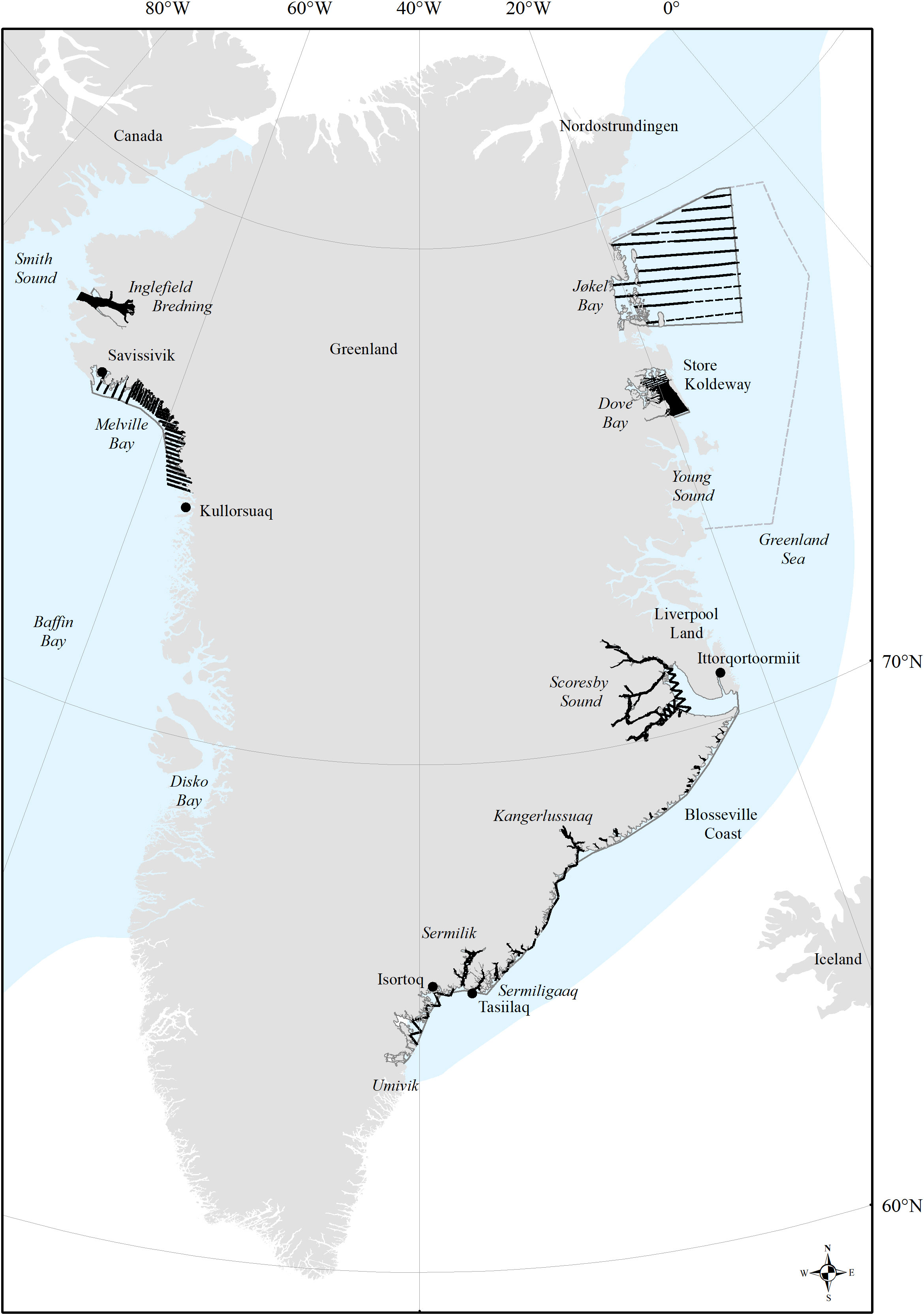
Figure 1 Distribution of effort on the narwhale summering grounds (delimited by grey line) in West Greenland (Inglefield Bredning and Melville Bay), Northwest Greenland (Jøkel Bay and Dove Bay) and East Greenland (Scoresby Sound to Umivik) with place names mentioned in the text. Black lines in bold indicate realized effort. Blue colored area indicates overall narwhal distribution in all seasons.

West Greenland

Inglefield Bredning was surveyed with transects aligned north-south from coast to coast and side fjords (Academy Bay and Bowdoin Fjord) were surveyed in a zig-zag manner between 15 and 21 August in 2007 following survey design described in Heide-Jørgensen et al. (2010). In 2019, between 21-27 August, the survey was repeated covering the same area and transects. The distance between transects in the western and eastern stratum in Inglefield Bredning was 2km and 1.2 km, respectively (Figure 2). Every other transect was covered during each survey day.

Figure 2

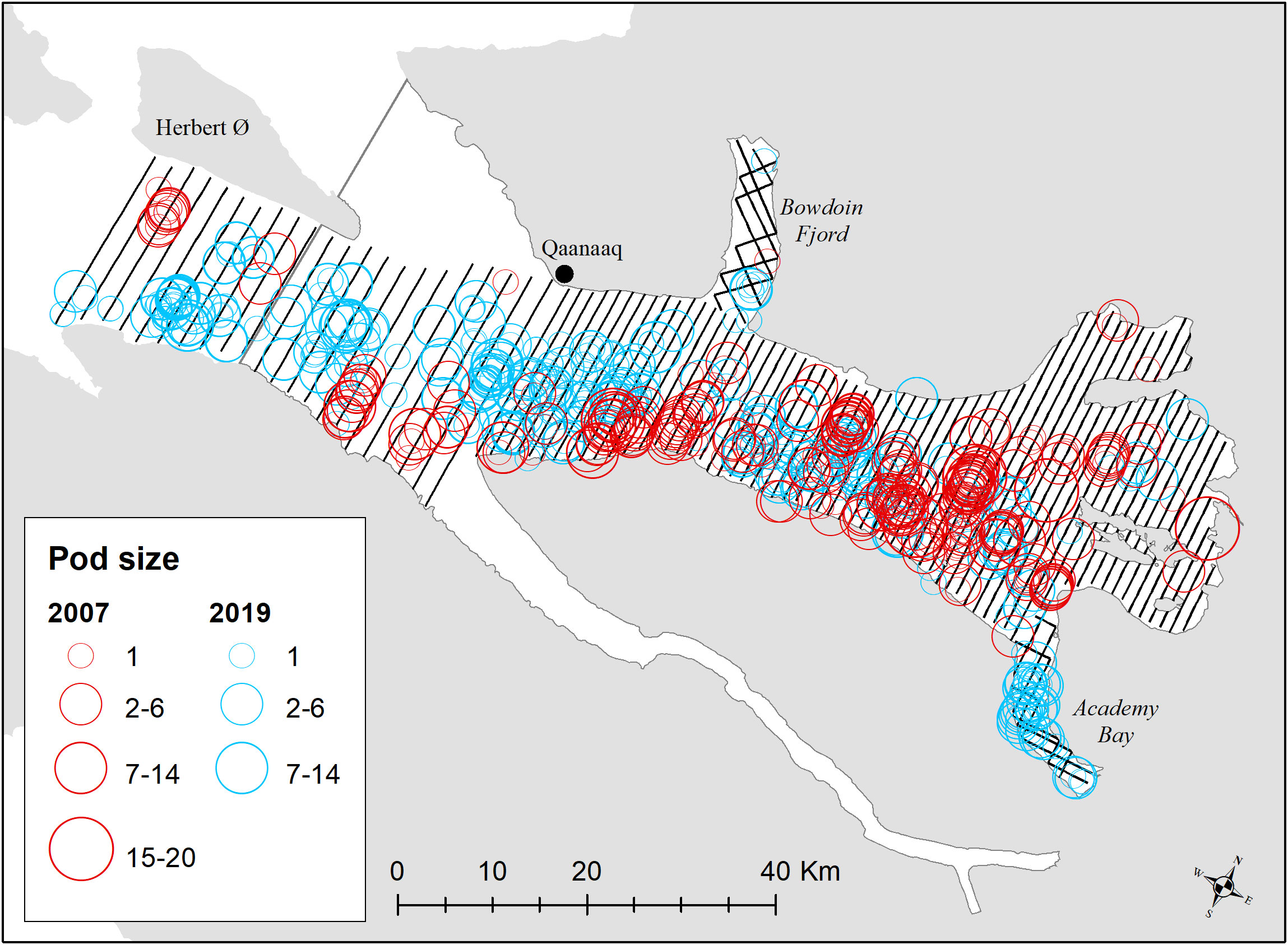
Figure 2 Transects on effort for surveys in Inglefield Bredning with strata delineation outlined in grey. Distribution of sightings of narwhals are shown in red (2007) and blue (2019).

In Melville Bay, four strata were identified to cover narwhal distribution and the two southern strata were surveyed by transects aligned east-west and the two northern were surveyed by north-south transects, systematically placed from the coast to offshore areas crossing glacier edges and bathymetric gradients (Figure 3). Every other transect was covered during each survey day. Melville Bay was surveyed between 11-23 August in 2007 (Heide-Jørgensen et al., 2010), in 2012 the survey was conducted between 28 August – 1 September, in 2014 between 25-30 August and in 2019 between 27 August – 2 September.

Figure 3

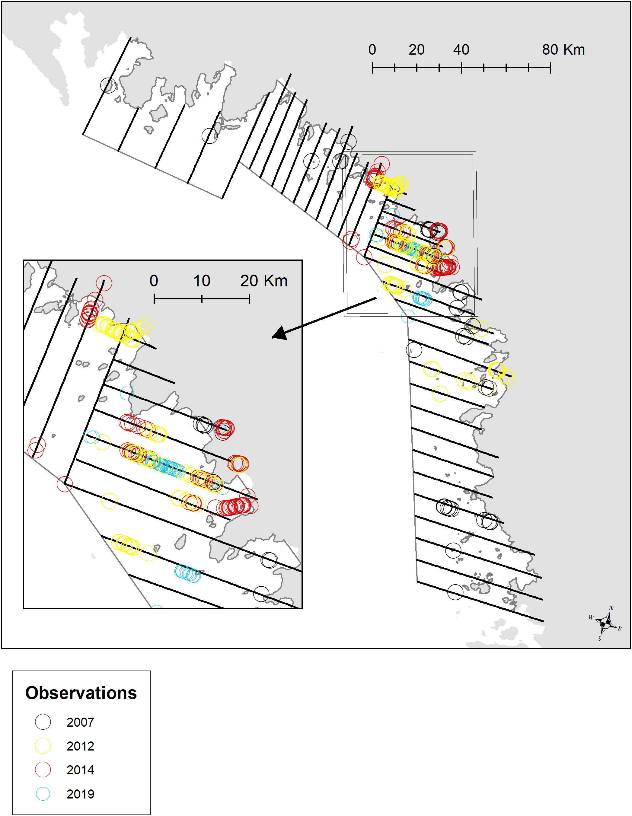
Figure 3 Transects on effort for surveys in Melville Bay with delineation of four strata outlined in grey. Distribution of sightings of narwhals are shown in black (2007), yellow (2012), red (2014) and blue (2019). Insert show the main distribution area in the central part of the bay.

East Greenland

Southeast Greenland is divided into three main regions. The fjord system of Scoresby Sound and the fjords and bays along the Blosseville Coast comprise one region, the Kangerlussuaq fjord system is a region, and the fjords and bays south of Kangerlussuaq to 64°N comprise a region. All were covered between 17 and 25 August 2016 (Figure 4). In 2008, the Kangerlussuaq fjord system, was treated as a stratum that is part of the Scoresby Sound region. Transect lines in the fjords were constructed in a zig-zag manner beginning at the outer coast and ending at the glacial front. A more intensive coverage than what was obtained at a previous survey in 2008 (Heide-Jørgensen et al., 2010) was attempted. In 2017, only the fjord system of Scoresby Sound was covered in the period 19 to 22 August (Figure 4).

Figure 4

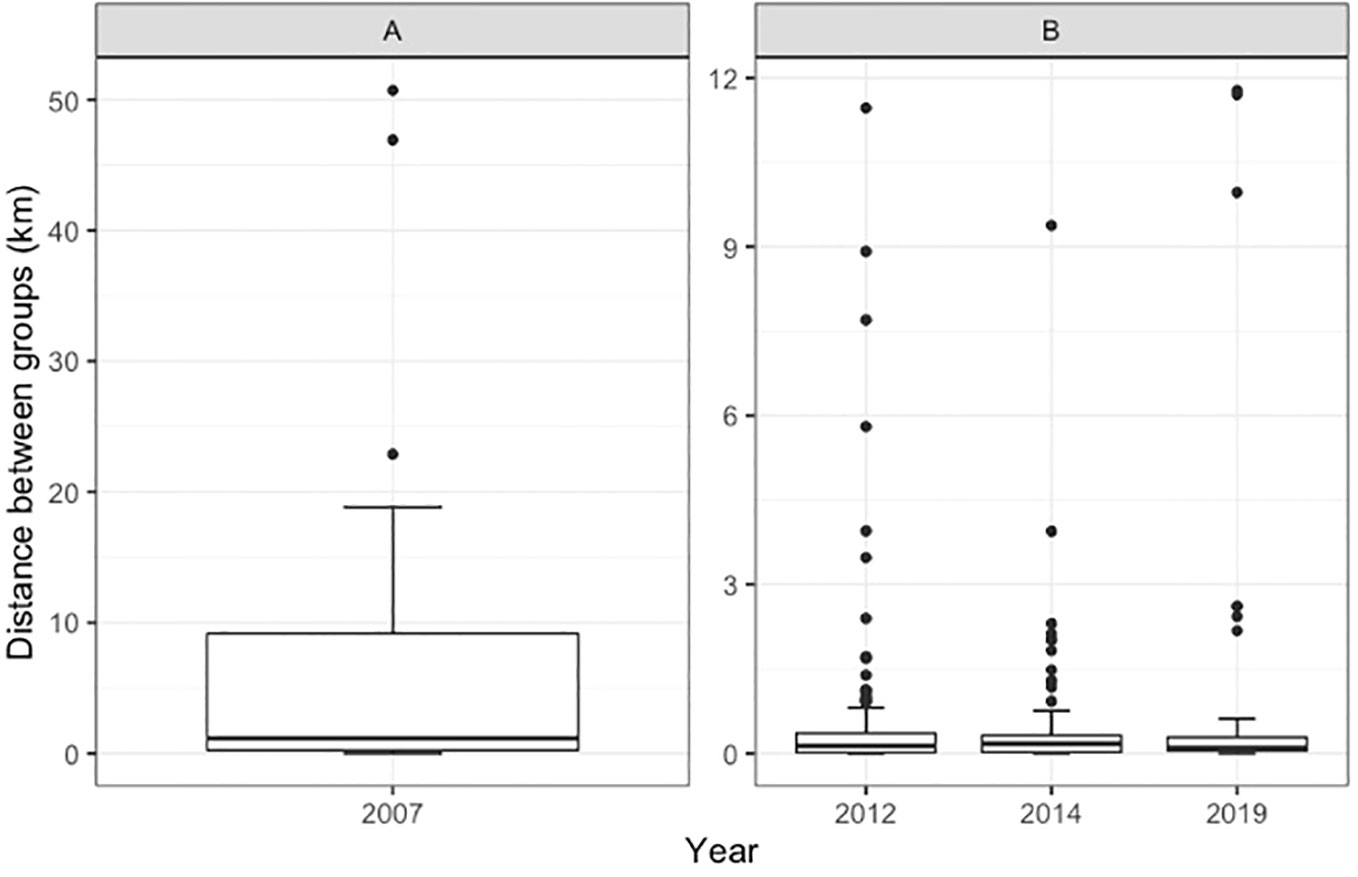
Figure 4 Distance between groups of narwhals in Melville Bay from 2007-2019. Note the large difference in the natural scale on the y-axis between year 2007 (A) and 2012-2019 (B).

In Northeast Greenland, The Greenland Sea was covered by evenly placed transects across strata from 73°N to 79°3N (post stratified at the eastern most sighting of narwhals) over the continental shelf between 23 August and 4 September 2017 (Figure 5). Two surveys in Dove Bay were conducted between August 30 and 3 September 2017 and between 1 and 5 September 2018. The initial coverage followed a zigzag design but due to the encounter of large densities of narwhals during the first survey, the design was changed to a design with evenly placed (4.7km apart) transects from coast to coast (Figure 6).

Figure 5

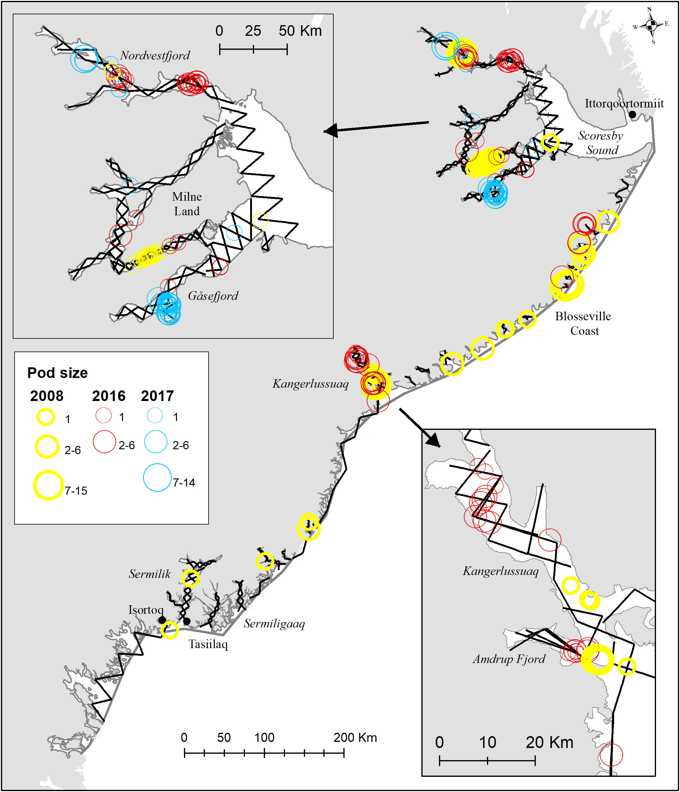
Figure 5 Transects on effort for surveys in Tasiilaq, Kangerlussuaq and Scoresby Sound with strata delineation outlined in grey. Distribution of sightings of narwhals are shown in yellow (2008), red (2016) and blue (2017). Inserts show the distribution areas in the main survey areas.

Figure 6

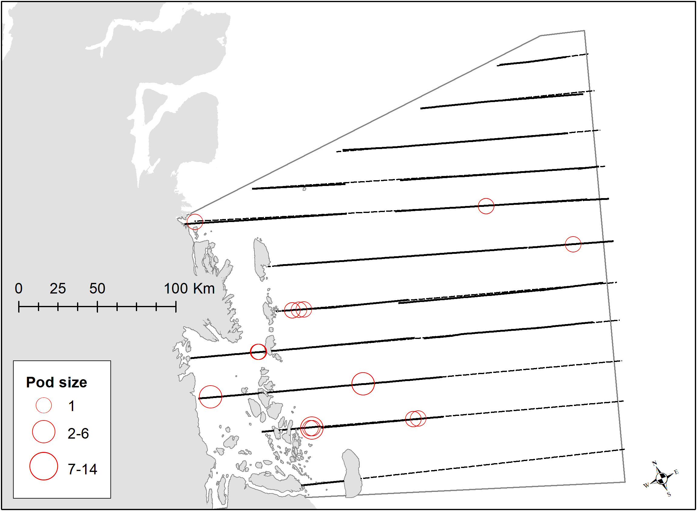
Figure 6 Transects on effort (black) and planned effort (dotted) for the survey in Jøkel Bay and a coastal part of the Greenland Sea, Northeast Greenland, between 23 August and 4 September 2017 with strata delineation outlined in grey. Distribution of sightings of narwhals are shown in red (2017). Jøkel Bay is stratified post survey as a proportion of the larger survey area indicated in Figure 1.

Recording of sightings

During the surveys, observers were instructed to concentrate their search view on the water surface closest to the plane, ahead and abeam to angles of 20 degrees where the field of view comprises ¼ of a circle between track line and abeam. Observers followed a specific data collection protocol, prioritizing certain information. This included recording sightings in a specific order of declination angle, group size (with minimum, maximum, and best guess estimates), time-in-view, and sex (certain or uncertain). They also noted the presence of a calf of the year or a 1-2-year-old calf. When animals were observed abeam, observers recorded declination angles using Suunto inclinometers in 2007-2014 and Geometers (electronic inclinometers) since 2016, which recorded roll, pitch, and yaw data when activated by a pushbutton (Hansen et al., 2020).

The recorded declination angles (α) for sightings abeam were then converted to radial distances using the equation d = altitude * tan(90-α), where d represents the distance. The altitude was calculated as an average value for each transect. Time-in-view (TIV) for a sighting was determined by measuring the time difference between the initial sighting of the animal(s) and when the sighting passed abeam converted into a forward distance assuming aircraft speed of 90 knots. It is assumed that all individuals in a group dive in synchrony and hence the number of animals in a group does not change while in view. Another assumption is that the group is not necessarily available in the entire time-in-view interval. If a group of narwhals had dived before abeam the TIV was set to a distance of 0m. Observers also documented the prevailing sighting conditions, such as sea state, ice coverage, and visibility. To identify double sightings, a post-survey analysis was conducted each day, considering the coincidence of time, distance, and group size. This standardized data collection methodology ensures consistency across surveys and enables accurate analysis of the survey data, allowing for the interpretation of narwhal distribution and abundance patterns.

Dealing with availability bias

During visual aerial surveys of marine mammals, there is an unknown proportion of animals that are submerged below a certain depth and thus not visible for detection. In the case of narwhals, this depth is assumed to be less than 2.5 meters (Richard et al., 1994; Heide-Jørgensen, 2004). We use the Hidden Markov Line Transect (HMLT) model of Borchers et al. (2013). This involves (a) fitting a two-state (available/unavailable) Markov model (MM) to data from depth recorders attached to individual whales in order to estimate whales’ patterns of availability, and (b) recording both the forward distance (y) and the perpendicular distance (x) for each sighting and modelling a two-dimensional detection hazard function h(x,y) instead of a one-dimensional detection function g(x). Figure 7 illustrates the key components of the model. The detection function g(x) is obtained by using hidden Markov model (HMM) methods to combine the MM for availability with the detection hazard function, h(x,y) (see Borchers et al., 2013 and Rekdal et al., 2014 for details).

Figure 7

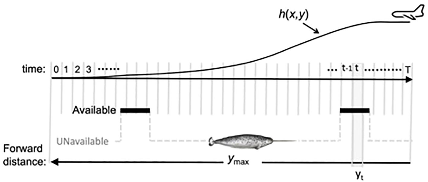
Figure 7 Schematic representation of the components of the HMLT modelM. The survey aircraft is moving from right to left and we model events within a forward distance y_max (meters) of the aircraft. Animals enter this distance interval at time 0 and come abeam of the aircraft at time T. Time is divided into small intervals numbered 0 (when the animal enters at maximum forward distance) to T (when it comes abeam). These correspond to forward distance intervals (only interval y_t is shown). The observer in the aircraft has a discrete detection hazard function h(x,y), which for any perpendicular distance x, gives the conditional probability of detecting an animal in forward distance interval y, given that the animal has not yet been detected and is available for detection. Animals switch between being available (bold line segments) and unavailable (grey dashed line segments) and this process is modelled as a Markov chain The availability sequence is hidden (hence the name “hidden Markov model”); all that is observed is the forward distance and perpendicular distance at the time of first detecting an animal. The diagram shows h(x,y) only for one perpendicular distance x.

The rationale for using the HMLT method is that the probability of detecting an animal depends not only on the proportion of time that it is available, but where it becomes available relative to the observer and how long its periods of availability and unavailability are. The MM in (a) above models how long its periods of availability and unavailability are and the detection hazard function models how detection depends on where it becomes available. The HMLT method combines these to estimate the probability of detection and the abundance. It uses a bootstrap method to incorporate the uncertainty about the availability pattern and about the detection hazard, into estimates (see Borchers et al., 2013 and Rekdal et al., 2014 for details). We can also get estimates of the proportion of time animals are available, together with associated 95% confidence intervals, from the MM availability model in (a) above. In this case, the confidence intervals are obtained by using the inverse Hessian matrix of the fitted MM availability model to estimate variance.

Data on the diving patterns of narwhals, used to estimate the MM for availability in (a) above, were obtained from a Satellite Linked Time Depth Recorder (whale #3965, as described in Heide-Jørgensen et al., 2015; Heide-Jørgensen et al., 2017). This recorder was deployed on August 13, 2013, and retrieved on August 14, 2014, in Scoresby Sound (EG), providing an unprecedentedly long record of time-at-surface data over approximately 90 days. The data collection occurred at a resolution of 1Hz (one reading per second) with a precision of 0.5 meters (Mahn et al., 2019). A subsample of 12 days from this dataset was used to estimate the availability process for the present study. The MM for availability was estimated from the 12-day dataset of narwhal diving behavior between 6 am and 6 pm, and each day was treated as an independent realization of the availability process. The resulting confidence intervals offer insights into the variability of narwhal availability over the 12-day period.

Comparisons of the dive sequence data from this particular narwhal with a larger sample of narwhals equipped with time-depth recorders revealed no significant differences (Heide-Jørgensen and Lage, 2022). Whale #3965 displays a large variation of dives (and series of dives) that encompass, if not all, then a large proportion of different surface behaviors found in the greater sample size of all whales. Since there are minimal differences in the average surface time among narwhals in the larger sample size, the findings by Heide-Jørgensen and Lage (2022) suggests that the data from the specific narwhal (whale #3965) can be used as representative of narwhal diving patterns in general, enhancing the reliability of the HMLT model. To correct the at-surface abundance estimate obtained from a revised MRDS analysis of a survey conducted in Southeast Greenland in 2008, the average time spent at depths less than 2.5 meters was utilized (Heide-Jørgensen and Lage, 2022).

Development of abundance estimates

Conventional distance sampling (CDS) models were fitted to the perpendicular distance data using the R package Distance (Figures 8; 9; Miller et al., 2019). Hazard-rate and half-normal models were fitted, with combinations of bf, ss, or no covariates and either right or left (or both) truncation was chosen. The best model by AIC was a hazard-rate model with no covariates.

Figure 8

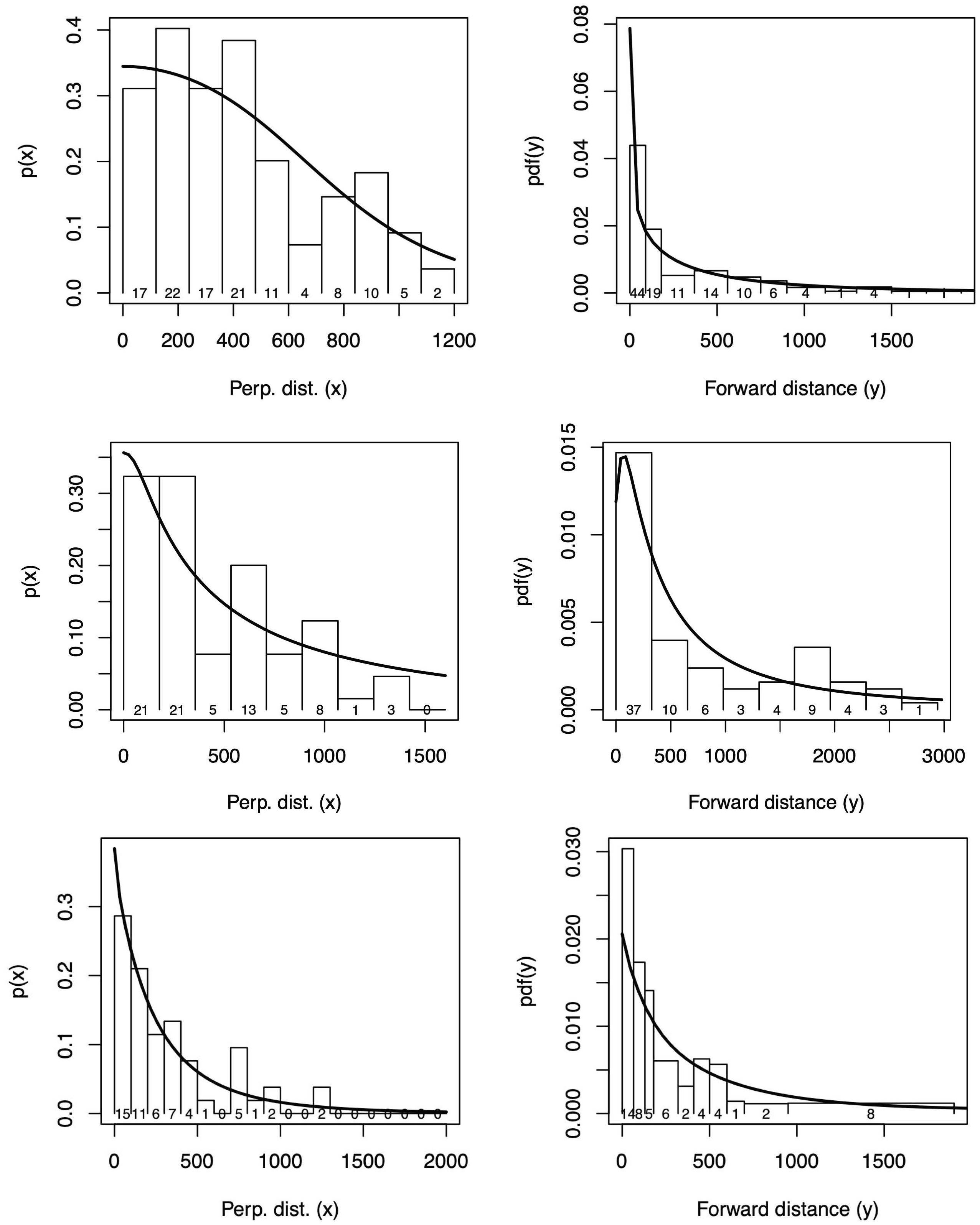
Figure 8 Perpendicular (left) and forward (right) distance data from the survey in 2012 (upper panel), 2014 (middle panel) and 2019 (lower panel) in Melville Bay. The detection function from the selected model is superimposed on a histogram of detection frequencies.

Figure 9

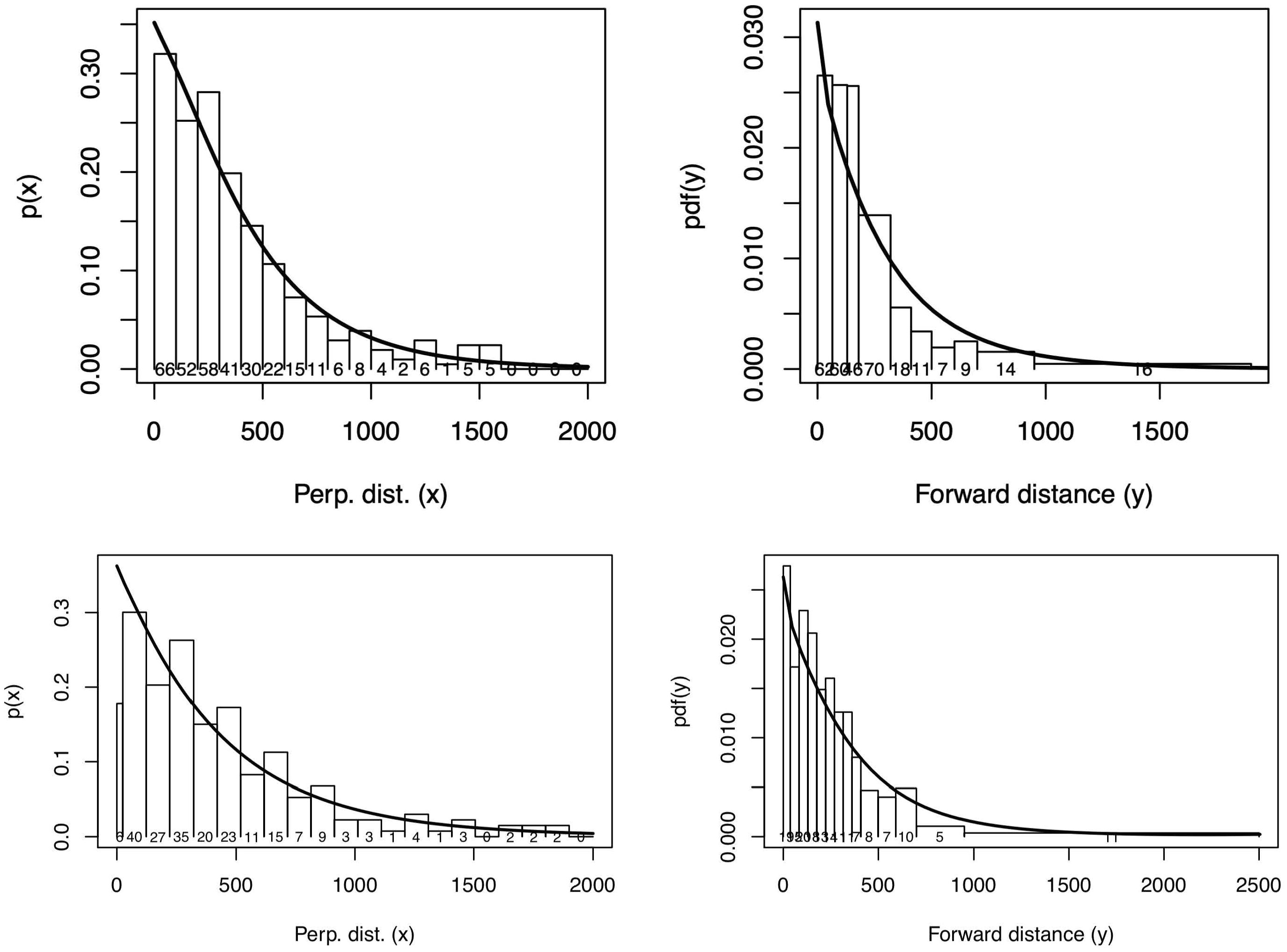
Figure 9 Perpendicular (left) and forward (right) distance data from the survey in 2019 in Inglefield Bredning (upper panel) and from the surveys between 2016 and 2018 in East Greenland (lower panel). The detection function from the selected model is superimposed on a histogram of detection frequencies.

The HMLT model of Borchers et al. (2013) was fitted to the sightings data, using the R package hmltm (available here: https://github.com/david-borchers/hmltm) and the MM for availability was fitted to the time depth recorder data from whale #3965. Unlike conventional distance sampling (CDS) methods that assume certain detection at perpendicular distance zero, regardless of whether the animals are within or below 2 meters of water, this method requires the much weaker assumption that the probability of detecting an animal that is at radial distance zero and is available, is 1.

By incorporating both the perpendicular (x) and forward (y) distances at which animals were detected and considering the availability process model, this approach provides more reliable estimation of the probability of detection than methods that use perpendicular distance only (see Borchers et al., 2013). The method accounts for both availability bias, which is addressed through the MM for availability, and imperfect detectability of available animals, which is addressed through the 2-dimensional detection hazard model, h(x,y). It does not require that both perpendicular (x) and forward (y) distances are observed for all sightings, but it does require that both distances are observed for some sightings.

Perception bias was estimated most all surveys using MRDS methods. To implement the method, the double-observer data collected during the surveys were converted to single-observer data. The two observers were treated as a single observation platform, so if an animal was detected by one or both observers, it was considered as a single sighting by the combined platform. By using these data with the HMLTM, we estimate g(0) for the combined observer platform under the assumption that if an animal is available for detection and at radial distance zero, at least one of the observers will detect it. (This replaces the MRDS assumption that the two observers’ detections are independent - an assumption that is violated by animals being available according to a random process, because in this case both observers tend to see the more available animals and both tend to miss the less available, or unavailable animals.)

The surveys conducted in East Greenland resulted in a limited number of narwhal detections. To enhance the accuracy of the detection functions, data from all surveys conducted in East Greenland, as well as a survey conducted in the winter in the North Water polynya in West Greenland in 2018 (which included 23 sightings), were included in the analysis. Preliminary examination of the distribution of distances revealed no significant difference between the winter and summer surveys. This suggests that the detection patterns remained consistent across seasons. Furthermore, three out of the four observers were consistent across all surveys. To improve the detection functions, a common detection function was fitted by combining the sightings from the seven surveys. Detection function parameters were estimated by maximizing likelihood Equation (5) of Borchers et al. (2013), as described by Rekdal et al. (2014). The availability models and detection hazard models are described below.

Forward and perpendicular distances to sightings were available for (at least some) sightings on the 2012-2019 surveys. In these cases, the following four forms of detection hazard function model given below were considered (Model name appears in brackets next to the model definition). We can incorporate covariates (z) into the scale parameter(s) of the detection hazard models. In this case, we write the detection hazard as h(x,y,z) instead of just h(x,y) as outlined above. The models differ in their shapes. Models IP and EP1 are the least flexible in that they have only one scale parameter ($\sigma$(z)) that determines the range of the functions in both the x- and the y-dimension, and one shape parameter ($\gamma$) that determines the shape in both dimensions. Model EP2 is more flexible as it has a single scale parameter, but separate shape parameters for the x- and y-dimensions ($\gamma$_x and $\gamma$_y). Model EP2x is most flexible, as it has separate scale parameters and separate shape parameters for each dimension.

$$h(x,y,z)={\left(\frac{\sigma (z)}{\sqrt{\sigma (z)+x^2+y^2}}\right)}^{\gamma }(\text{Model IP})$$

$$h(x,y,z)=exp\left\{-{\left(\frac{x}{\sigma (z)}\right)}^{\gamma }-{\left(\frac{y}{\sigma (z)}\right)}^{\gamma }\right\}(\text{Model EP}1)$$

$$h(x,y,z)=exp\left\{-{\left(\frac{x}{\sigma (z)}\right)}^{{\gamma }_x}-{\left(\frac{y}{\sigma (z)}\right)}^{{\gamma }_y}\right\}(\text{Model EP}2)$$

$$h(x,y,z)=exp\left\{-{\left(\frac{x}{{\sigma }_x(z)}\right)}^{{\gamma }_x}-{\left(\frac{y}{{\sigma }_y(z)}\right)}^{{\gamma }_y}\right\}(\text{Model EP}2\text{x})$$

West Greenland

For each year’s survey, the best model form among these was chosen on the basis of AIC after fitting each model with no covariates to data from each year. The chosen model form was then fitted using various combinations of the available covariate data (bf: Beaufort sea state, ss: group size, and in some years wait: waiting time since last sighting), and the best model chosen on the basis of AIC.

East Greenland

The best model form among these was chosen on the basis of AIC after fitting each model with no covariates to data from all years simultaneously (with no year effect). The chosen model form was then fitted to data from all years using combinations of covariates (again with no year effect), and the best among these was selected on the basis of AIC. This model was then compared to a model fitted to all years’ data and including a year effect (i.e. year as a covariate). The best of these two models was selected on the basis of their AIC values. The estimated parameters from this model were used to estimate detection probability, p(x), using Equation (1) of Borchers et al. (2013), and the expression for p(x) that is given below Equation (1) of that paper.

Goodness of fit in the perpendicular distance (x) and forward distance (y) dimensions was evaluated using Kolmogorov-Smirnov goodness of fit tests. When there was evidence of rounding of forward distances, this test is not applicable and a Chi-squared goodness of fit test, using data grouped into intervals, was used to test goodness of fit in the forward dimension instead.

Abundance and mean group size estimation on surveys with forward distances

Group abundance and animal abundance in each of the survey strata was estimated using the following Horvitz-Thompson-like estimators

$${\widehat{N}}_g=\frac{A}{a}{\displaystyle \sum _{i=1}^n\frac{1}{{\displaystyle {\int }_0^W{\widehat{p}}_i(x, z_i)\frac{1}{W}dx}}}$$

and

$$\widehat{N}=\frac{A}{a}{\displaystyle \sum _{i=1}^n\frac{s_i}{{\displaystyle {\int }_0^W{\widehat{p}}_i(x, z_i)\frac{1}{W}dx}}}$$

where W is the perpendicular truncation distance, A is the stratum area, a is the covered area (a = $2WL$, where L is total transect length), s_i is the group size of the ith detected group, n is the total number of sightings in the stratum and ${\widehat{p}}_i(x, z_i)$ is the estimated sighting probability of group i, with covariates $z_i$, evaluated at perpendicular distance x. Group size of each sighting is the average group size from the front and rear observer. If a sighting was assigned a certain group size from one observer and a best guess from the second observer, the group size from the observer with the certain group size was used. If both observers had a sighting where group size was a best guess then the average of the two was used. Mean group size in each stratum was estimated by $\widehat{E}[s]={\widehat{N}}_g/\widehat{N}$ and estimated abundances in strata were summed to provide regional abundance estimates.

Variance and confidence interval estimation on surveys with forward distances

Variances and 95% confidence intervals of abundance, mean group size and related parameters were estimated using a two-stage bootstrap procedure, in which each bootstrap iteration is as follows:

Stage 1: Resample parametrically from the estimated information matrix of the estimated MM availability model parameters of each of the 12 available fitted MMs (one for each day) for narwhals.

Stage 2: Resample transects with replacement within each stratum, together with the sightings made on the resampled transects. Re-estimate detection hazard function parameters by maximizing likelihood Equation (5) of Borchers et al. (2013), conditional on the resampled MMs for animal availability; re-estimate abundance, mean group size and related parameters, as outlined above.

Variances were estimated by the variance of the estimates from 250 (Melville Bay and Inglefield Bredning) and 500 (East Greenland) bootstrap samples of each of the quantities of interest. Confidence intervals for abundance were obtained from these estimates using the coefficient of variation estimated from the bootstrap procedure above and assuming log-normality of the abundance estimator.

Alternative variance and confidence interval estimation in Melville Bay in 2019

Because of the extreme clustering of detections in Melville Bay in 2019 (the majority of the 54 detections made on the survey were on a single transect), we used Method O1 of Fewster et al. (2009) to provide an alternative estimate of the variance of the encounter rate on this survey (in the Central stratum, which is the only stratum with any detections). The Fewster variance estimator (O1) is a post-stratification method in which the survey stratum is subdivided into a set of overlapping substrata consisting of each pair of adjacent track lines. The variance in each substratum is estimated and then the variances of the substrata are summed and averaged to estimate the variance for the stratum. This approach accounts for the spatial distribution of variance which is largely limited to the region of the higher density clumped animals. To incorporate this alternative estimate of variance in the abundance estimate, we calculated the alternative estimate of the CV of the abundance estimates as

$${\widehat{CV}}_{O1}{(\widehat{N})}^2={\widehat{CV}}_{Boot}{(\widehat{N})}^2-{\widehat{CV}}_{Boot}{(\widehat{n/L})}^2+{\widehat{CV}}_{O1}{(\widehat{n/L})}^2$$

where ${\widehat{CV}}_{O1}{(\widehat{N})}^2$ is the alternative estimate of the squared CV of estimated abundance ($\widehat{N}$), ${\widehat{CV}}_{Boot}{(\widehat{N})}^2$ is the bootstrap based estimate (as 2.1.3 above) of the squared CV of estimated abundance, ${\widehat{CV}}_{Boot}{(\widehat{n/L})}^2$ is the bootstrap based estimate of the squared CV of the encounter rate (n/L), and ${\widehat{CV}}_{O1}{(\widehat{n/L})}^2$ is the estimate of the squared CV of the encounter rate, using method O1 of Fewster et al. (2009).

Methods for surveys without forward distances

In the case of the 2007 surveys in Melville Bay and Inglefield Bredning, West Greenland, no forward distances were available. In this case, the methods of Borchers et al. (2013) cannot be used. Instead, multiple covariate distance sampling methods (R package Distance; Miller et al., 2019) were used to estimate abundance under the assumption that g(0)=1 and g(0) was estimated using the method of Laake et al. (1997) using the MM availability estimates described above. The distance sampling estimate of abundance was divided by this g(0) to “correct” for availability bias. Confidence intervals for abundance were obtained by calculating the coefficient of variation (CV) of the “corrected” estimate as the square root of the sum of the squared CV obtained from the package Distance and the squared CV of the g(0) estimate, and assuming abundance to be lognormally distributed. An estimate of the CV of the g(0) estimate was obtained by bootstrap.

The method of Laake et al. (1997) requires a forward distance to be specified, beyond which available animals cannot be detected and within which they are assumed to be detected with certainty. There is in reality no such distance, because the probability of detecting an available animal decreases smoothly with increasing forward distance and it is only at very short forward distances that detection of available animals is certain. Selection of a forward distance to use with the method is therefore somewhat subjective. We estimated the coefficient of variation of the g(0) estimate from Laake’s method by bootstrapping (1,000 replicates) the availability data (Figure 10) and recalculating Laake’s g(0) for each bootstrap replicate. The squared CV of the “corrected” abundance estimate (that from the CDS model divided by the g(0) estimate) was obtained as the sum of the square of the CV of the g(0) estimate and the square of the CDC abundance estimate. Abundance estimates were obtained separately in regions Inglefield Bredning and Melville Bay in 2007, but using the same detection function, fitted to all sightings.

Figure 10

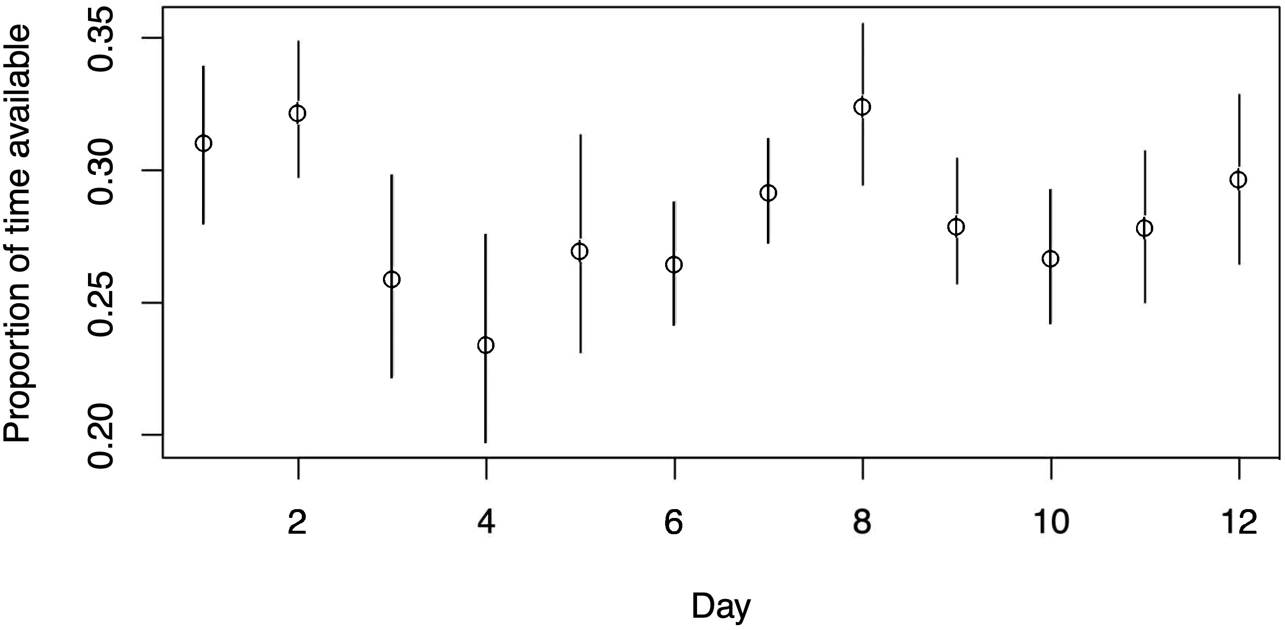
Figure 10 The estimated proportion of time whales are available, together with 95% confidence intervals, for each of the 12 days of depth tag data to which HMMs were fitted.

Corrections of abundance from Southeast Greenland 2008

Abundance of narwhals in East Greenland has previously been estimated by Heide-Jørgensen et al. (2010) using a MRDS analysis. Here we update the MRDS estimate of abundance by corrected transect line measurements, cartographically updated strata areas and a new correction for availability of 0-2 m depth using dive data from the same individual as presented in this paper (29.62%, CV= 0.20, Heide-Jørgensen and Lage, 2022).

Results

Distribution

West Greenland

Both Inglefield Bredning and Melville Bay were divided into four strata each for survey design. In Inglefield Bredning, the surveys conducted in 2007 and 2019 revealed a similar distribution of narwhal sightings, however, in 2019, a notable increase in sightings was observed in Academy Bay (Figure 2). The presence of sightings in the westernmost part of the main fjord stratum suggests the possibility of more whales residing outside the surveyed region.

In 2019 in the Melville Bay the narwhal sightings were concentrated in the central stratum, which contrasts significantly with the distribution in 2007 when narwhals were detected in all four strata (Figure 3). In 2012, narwhals were observed in three strata, and in 2014, sightings occurred in two strata. The area of strata where narwhals were observed decreased from approximately 16,400 km² in 2007 to 2,610 km² in 2019, indicating an 84% decrease in area usage (Table S1). The average group size of narwhals, ranging between 2.4 and 3.3 individuals, remained relatively consistent over the years. However, the distance between groups showed a significant decline, from an average of 6.8 km with substantial variation in 2007 to 0.6 km with minimal variation in 2012 (Figure 4). Since 2014, all sightings were within close proximity (<1 km) of neighbouring sightings.

East Greenland

East Greenland was divided into several regions defined as The Greenland Sea, Dove Bay, Scoresby Sound, Kangerlussuaq and South of Kangerlussuaq. All regions revealed limited observations of narwhals that were found scattered between latitudes 65-79°N, with relatively higher concentrations in specific regions such as the Greenland Sea (Jøkel Bay and Dove Bay), Scoresby Sound and Kangerlussuaq fjord systems. In 2008 narwhals were detected in all major fjord systems such as Sermilik, Kangerlussuaq, and Scoresby Sound, as well as in several other fjords, bays, and inlets along the Blosseville Coast. These areas include all the hunting grounds that have been in use since the turn of the century in East Greenland and hence narwhals were present at each hunting locality [Scoresby Sound fjord system and areas south to Isortoq (around 65°N, Figure 5)].

In 2016, a total of 66 unique sightings of narwhal groups were recorded in 9 strata, with more than half of the sightings found in the Scoresby Sound region. Out of the 37 fjords along the Blosseville Coast, a random sample of 15 fjords was surveyed, and narwhals were detected in 3 of them. In Scoresby Sound, narwhals were mainly found in Nordvestfjord, Inner Gåsefjord, and around Milne Land. The majority of sightings consisted of single animals, and the largest groups (with a group size of 6) were recorded in the Kangerlussuaq and Nordvestfjord strata. Since 2008, no whales have been detected south of Kangerlussuaq, and the regions where narwhals have been observed decreased from approximately 30,000 km2 in 2008 to 19,800 km2 in 2016, representing a decrease in area usage of 34% over eight years (Table S1). In 2008, the southernmost sightings of narwhals were made at latitudes 65.3°N and at 70°N in 2016. Both the maximum and average distances between the closest narwhal sighting decreased from 71 km to 48 km and from 6 km to 3 km, respectively. No significant difference was detected in group size between the two survey years, with an average of 2.2 (CV=0.25) in 2008 and 1.3 (CV=0.06) in 2016. In 2017, only the Scoresby Sound fjord system was surveyed (Figure 5).

Narwhals North of Scoresby Sound were concentrated in the Greenland Sea in the coastal area of Jøkel Bay between 78-79°N, an area dominated by the large (80 km long) 79°N glacier, as well as in Dove Bay between 76-77°N (Figures 6, 11; Table 1). Fifteen sightings of narwhal were obtained during the survey in the offshore area of the Greenland Sea and an abundance estimate in a post-stratified stratum, in the northern part of a larger multi-species survey, was developed. In addition, there was a relatively high density of narwhals in Dove Bay (Figure 11; Table 1).

Figure 11

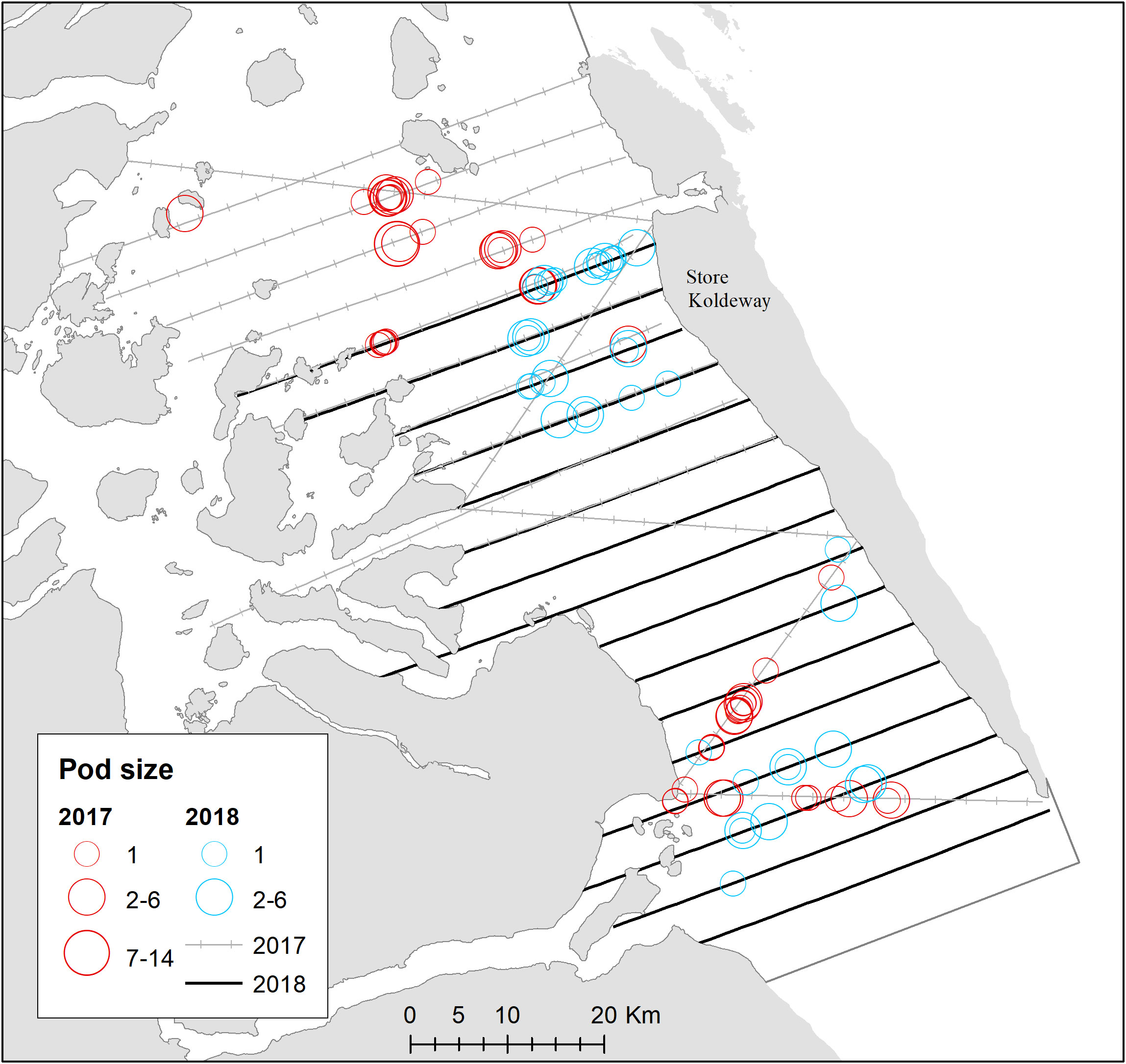
Figure 11 Transects on effort for surveys in Dove Bay. Distribution of sightings of narwhals are shown in red (2017) and blue (2018). The two northern most zig-zag lines were not used for abundance estimation.

Table 1

Table 1 Summary of survey effort and number of sightings seen by all platforms for each survey.

Abundance estimation

Data on effort and sightings per region are given in Tables 1, 2 and in Supplementary Table 1. Multiple surveys were conducted in each region, with transects covering alternate sections on individual survey days. Each transect was treated as an independent sample for analysis. Differences in duplicate sightings for perpendicular distances and in group sizes were examined and no systematic patterns were apparent. It was therefore decided to use the average distance and group size between front and rear observer. The combined perception bias was estimated to be between 0.96-0.98 for the various surveys. After exploratory analysis, detections were left-truncated for some surveys at 50 to 150m perpendicular distance. For some surveys there seems to be a paucity of detections at small perpendicular distances, something that is not uncommon with aerial surveys, especially in surveys with few sightings where observers tend to spend more time searching farther from the track line. Detections were also right-truncated at perpendicular distance 2000m.

Table 2

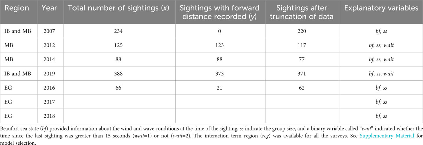
Table 2 Overview of sightings and explanatory variables with regions Inglefield Bredning (IB), Melville Bay (MB), East Greenland (EG).

West Greenland

No forward distances were recorded for the survey in Inglefield Bredning and Melville Bay in 2007 (Table 2). To help decide what forward distance we should use for Laake’s method with the 2007 data, we considered the estimates of g(0) obtained from the 2012, 2014 and 2019 surveys in Melville Bay (see below) that were obtained using the method of Borchers et al. (2013). The g(0) from Laake’s method is shown in Figure 12 as a function of specified forward distance, together with the g(0) estimates from the 2012, 2014 and 2019 surveys (horizontal lines). Guided by Figure 12, we decided to use a forward distance of 500m to calculate a g(0) with Laake’s method, to “correct” the CDS estimate from the 2007 data. Mean g(0) was estimated to be 0.377 (CV=0.013).

Figure 12

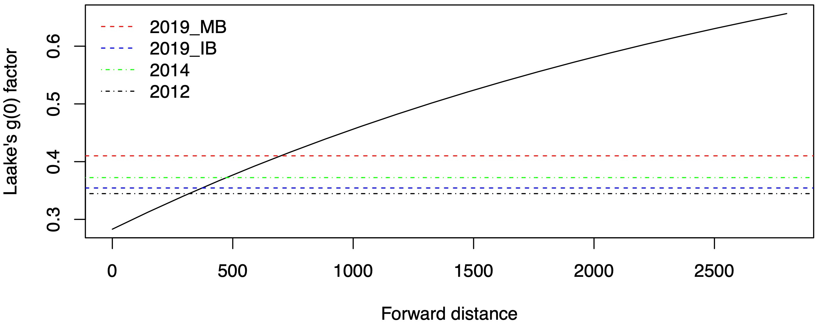
Figure 12 Laake’s g(0) estimate using the mean proportion of time available that is shown in Figure 8, as a function of forward distance (meter). g(0) estimates from the 2012, 2014 and 2019 survey in Melville Bay (MB) and in 2019 in Inglefield Bredning (IB) are shown as horizontal lines.

The recorded forward distances of sightings from the survey in Melville Bay in 2012 suggested rounding to zero of sightings at small forward distances (Figure 8). To deal with this, the method of Borchers et al. (2013) was extended to accommodate grouped data within some specified forward distance of zero, and exact distances beyond this. This model was fitted both with grouped data out to 150m forward distance, and without grouping. The fits yielded similar results, with abundance estimates differing by no more than 1, and the ungrouped data fit was used. The rounding does however invalidate the Kolmogorov-Smirnov goodness of fit test, and instead a Chi-squared test was used to asses goodness of fit.

Model selection by AIC suggests that a hazard detection model with bf and wait affecting the scale parameter in the x-dimension and no covariates in the y-dimension should be used (Figure 8). The fit in the x-dimension is good (Kolmogorov-Smirnov p-value = 0.85) while that in the y-dimension is not (K-S p-value = 0.005). The badness of fit in the y-dimension occurs primarily within about 100m of the origin. A Chi-squared test with intervals defined by the histogram intervals suggests grouping at distances close to zero (p=0.02).

The perpendicular distance distribution of the sightings from the survey in Melville Bay in 2014 showed a decline as distance approached zero (Figure 8), suggesting that perhaps animals were missed closer to the track line due to obstructed forward or downward view. This decline led to poorly-fitting detection function models and as a result left-truncation at 150 m was implemented. Model selection using AIC showed that a detection hazard model IP with ss as an explanatory variable provided the best fit and it was used with the availability data (Figure 10). The fit was adequate in both the x-dimension (K-S p-value = 0.60) the and y-dimension (K-S p-value = 0.24, Figure 8).

For the survey in Inglefield Bredning and Melville Bay in 2019 the detection hazard model was found by AIC to fit best, and a range of combinations of variables were considered for the scale parameter in which ss and bf and their interaction with region (reg) affected the scale parameter in the y-dimension, and ss and its interaction with region (reg) affected the scale parameter in the x-dimension (Figure 8). This is equivalent to separate models for each region, with ss and bf affecting the scale parameter in the y-dimension (differently in each region) and with ss affecting the scale parameter in the x-dimension (differently in each region).

For Inglefield Bredning 2019 the fit was adequate in the x-dimension (K-S p-value = 0.74) but the fit in the y-dimension was not satisfactory (K-S p-value = 0.001, Figure 9). With 332 sightings there is considerable power to reject the null hypothesis even for small deviations from expected value, hence the low p-value despite the fit not being visually very bad. For Melville Bay 2019 the fit was adequate in both the x-dimension (K-S p-value = 0.99) and the y-dimension (p-value = 0.74, Figure 9). We used the method O1 of Fewster et al. (2009) to estimate the encounter rate variance.

East Greenland

The likelihood of Borchers et al. (2013) was extended to include detections with no y by adding a new marginal component to the likelihood, in which y is integrated out of the likelihood for each detection. Beaufort sea state (bf) and group size (s) were incorporated by allowing the x and/or y scale parameters of the detection hazard function models (${\sigma }_x$ and ${\sigma }_y$) to depend on the covariates bf and/or ss. The data from East Greenland 2016-2019 were combined and the fits were acceptable for both x-dimension (K-S p-value=0.3160) and the y-dimension (Chi-Square p-value=0.1130, Figure 9).

Corrections of abundance from Southeast Greenland 2008

The MRDS analysis used to estimate abundance of narwhals from a survey in Southeast Greenland in 2008 was reanalyzed using corrected transect lengths and strata areas but otherwise using the same MRDS approach as described by Heide-Jørgensen et al. (2010). Recalculation of the 2008-survey with the corrected transect lengths and strata areas changed the individual abundance estimate, corrected for perception bias, to 817 animals (CV= 0.48; 95% CI 328-2035). The at-surface estimate of 817 animals is considerably lower than the old estimate of 1353 (CV=0.50) animals. Correction with the new availability correction factor from whale #3965 gave an estimate of 2758 narwhals (CV= 0.52; 95% CI= 1060-7200) in Southeast Greenland. The point estimate corrected for availability bias of 2758 individuals is also lower than the old estimate of 6444 individuals (C=0.51; 95% CI=2505-16,575).

Trend abundance

There was no statistically significant trend in abundance in Melville Bay and Inglefield Bredning so it cannot be rejected that there has been no change in abundance between 2007 and 2019. For Melville Bay, the test has low power because of the high variance in 2007 and 2019. The confidence interval for Melville Bay in 2019 in particular is wide, and this is due mainly to the high CV of the encounter rate (68%), which is due in turn to the majority of the 54 sightings made on the survey being on a single transect. If we use the Method O1 of Fewster et al. (2009) the CV of the encounter rate is reduced to 42% and the confidence interval for abundance is reduced in width by about 30%, but the null hypothesis of no change in abundance between 2007 and 2019 still cannot be rejected. In East Greenland both Kangerlussuaq and Scoresby Sound showed significant declines in abundance (Table 1).

Discussion

Subsistence hunt of narwhals occur at their summer grounds in West Greenland and Southeast Greenland and surveys at regular intervals are necessary for assessing the sustainability of the hunt. In this paper, we present the most recent distribution patterns and abundance estimates of narwhals from these surveys. We specifically focus on reducing the impact of the availability correction, hence adjusting for diving animals, by using Hidden Markov Line Transect Models (HMLTM) to estimate total abundance. To ensure comparability in trends of abundance in the different regions, we reanalyze previous survey estimates using the same methods.

When estimating total abundance of narwhals in a region, it is important to account for the fact that not all individuals are available at the water surface for detection during surveys. In the past, this correction was achieved by multiplying the at-surface abundance with an instantaneous correction factor derived from data obtained from satellite transmitters deployed on the whales. These transmitters provided information on the average time an individual narwhal spent in the 0-2m depth range, which is the depth range within which they are assumed to be detectable by observers (Heide-Jørgensen et al., 2010). The HMLT model requires complete high-frequency sampling of the dive profiles of narwhals to estimate the hidden-state where the whales are unavailable for detection (depths below 2m). Survey specific data on the time the water surface is under surveillance by the observers is then included to estimate the forward detection probability.

Dive data from only one individual were included in the availability matrix, which may lead to speculation that this particular whale may not represent the full spectrum of all surfacing behaviors exhibited by narwhals. In the paper authored by Heide-Jørgensen and Lage (2022), a comparison of the surfacing behavior of the whale we are using in the abundance estimation paper (whale #3965) and several other whales are presented. This comparison revealed minimal differences in the average surface time among seven animals with shorter-duration time series and the one we have used (#3965). This is partly explained by the fact that all narwhals are subject to physiological constraints regarding the time they can stay submerged and the number of dives they can make per hour. Interestingly, whale #3965 had the same number of dives per hour as a significant number of whales previously tagged from both Canada and Greenland. Whale #3965 displays a large variation of dives (and series of dives) encompassing all types of dives found in the greater sample size of all whales (Heide-Jørgensen and Lage, 2022). We adjust abundance for diving groups of narwhals with the diving behavior of an individual animal assuming that the group act as an entity, meaning the individuals in a group appear and disappear in synchrony.

The use of HMLTM instead of MRDS introduces two key changes to the abundance estimation process. Firstly, the HMLTM uses the forward distances as well as the perpendicular distances to estimate detection probability. Secondly, the availability correction factor used in HMLTM considers not only the proportion of time whales spend in the 0-2m depth bin but also considers the variation in dive patterns and dive cycles. Despite having data from only one whale in this survey, the dataset still contains a sufficient number of dives (12 days with over 2000 dives) and dive types to generate an availability model that reflects the variety of patterns of availability well. In the HMLTM the availability bias is not a simple multiplier correction because the models were fitted to each day with depth data separately, treating depths< 2.5m as being available for detection, then treating these as independent samples from whale dive patterns, calculating the likelihood for each pattern, and then summing over these separate likelihood components (see Borchers et al., 2013 for details). This is equivalent to treating the whale availability pattern as a random effect in the model. The individual average proportions of time available each day varied from about 20% of the time to just over 30% of the time. By utilizing this availability model, the abundance estimation obtained through HMLTM yields a larger but more accurate estimated g(0) (the probability of detecting a whale at zero perpendicular distance). In contrast, previous surveys analyzed using the MRDS method in combination with an instantaneous availability correction factor may have exhibited a positive bias in their abundance estimates. This is explained in detail by See Borchers et al. (2013) for how use of an instantaneous correction factor can result in a negative bias in estimated detection probability, which in turn induces a positive bias in estimated abundance. The key idea is that when animals are available for more than an instant, their detection probability is higher than the proportion of time that they are available for only an instant. So, if you have an abundance estimate from a survey in which animals were available for more than an instant and you apply a correction to this abundance estimate that treats them as if they were available for only an instant, you adjust the proportion of diving animals by a factor that is too high.

The MRDS method can account for availability bias as well as perception bias, but only if animals go through many available/unavailable cycles while within detectable range, and not if some animals can be unavailable for the whole time they are within detectable range. In this survey, the maximum forward distance, y_max (see Figure 7), was chosen to be 2,400m, which is greater than the largest observed forward distance. The survey aircraft covers this distance in about 52 seconds. The mean time that narwhals are estimated (from the 12 dive depth datasets) to be unavailable in a single dive cycle ranges from 38 seconds to 216 seconds. The probability that a whale that is unavailable for 216 seconds is never available while within a detection window of 52 seconds is about 52% ((216-2*52)/216). It is therefore clear that a sizeable proportion of whales that are present could never be detected by the observers, and hence that an MRDS method could never correct for this availability bias.

West Greenland

The distribution patterns of narwhals in Inglefield Bredning demonstrate a widespread utilization of the fjord, with no significant differences observed between the two survey years, except for a higher concentration of sightings in the small side fjord, Academy Bay, during the survey in 2019. However, it is worth noting that both surveys had observation of narwhals at the most western transects furthers suggestion more narwhals may have been present beyond the surveyed area. The observed concentration of sightings in the inner part of Inglefield Bredning aligns well with previous aerial surveys conducted in the same area, as reported by Born et al. (1994) and Heide-Jørgensen (2004). This consistency indicates that a similar proportion of the narwhal population is likely to be available for surveying within Inglefield Bredning during all surveys conducted in August.

The re-analysis of abundance estimates from Inglefield Bredning in 2007 reveals a notable reduction in the estimated narwhal population size. The previous estimate using the MRDS technique yielded an abundance of 8368 individuals (with a confidence interval of 5209-13442). However, with the implementation of the HMLTM method, the revised estimate indicates a lower abundance of 4110 individuals (with a confidence interval of 2738-6168). The disparity in abundance estimates between the two techniques is somewhat attributed to the differences in estimation methods. However, the primary factor contributing to the change in abundance is the variation in the availability correction factor employed in the two years. Specifically, the availability correction factor was 0.21 (CV=0.09) in 2007 and 0.30 (CV=0.20) in 2019, as determined by Heide-Jørgensen and Lage (2022).

During all surveys conducted in Melville Bay, four strata covering the main distribution of narwhals were systematically covered. However, in the 2019 survey, narwhals were only found in the Central stratum, primarily in close proximity to land and glaciers. This indicates a significant shift in the area used by narwhals in Melville Bay over time. The analysis of presence/absence of whales in the four strata suggests a steady decline in the area utilized by narwhals in Melville Bay. The area used by the population decreased from 16,362 km² in 2007 to 2,610 km² in 2019. This reduction in area indicates a contraction of the narwhal’s range within Melville Bay. Furthermore, the distance between neighbouring sightings has also decreased over the years. Between 2007 and 2012, the distance between sightings became progressively closer. Since then, the majority of sightings have occurred within 1 km of each other, indicating a higher spatial aggregation of narwhals within the bay and in 2019, more than 70% of the sightings in Melville Bay were concentrated in one area (one transect). This concentration of sightings on one transect has a substantial impact on the overall abundance estimate and introduces a higher variance into the survey results. To address the challenge of estimating variance in clumped distributions, an alternative method of estimating the variance (Fewster et al., 2009) reduced the variance observed in 2019 by approximately 20%.

While the density of narwhals in Melville Bay is generally low compared to other summer grounds, it is important to note that Melville Bay differs from those areas. Typically, narwhal summer grounds consist of narrow fjords or inlets bordered by coastlines on three sides. In contrast, Melville Bay has an open and elongated coastline, allowing narwhals to freely move north and south as well as offshore to the west. However, during the summer, narwhals tend to congregate in front of glaciers within the Melville Bay and are rarely observed further offshore. Although large groups of narwhals are still present in Melville Bay, their distribution is now concentrated in a smaller area. This concentration may create the impression among local hunters that the population is still large. However, the observed monotonic decline in the coastal area utilized by narwhals between 2007 and 2019 suggests a potential significant decline in the population.

The abundance estimates obtained from the surveys conducted between 2007 and 2019 were used to assess the trend in narwhal abundance in Melville Bay and Inglefield Bredning, but the trend in abundance was not significantly different from zero, indicating that there is no clear evidence of a significant increase or decrease in narwhal abundance in Melville Bay and Inglefield Bredning over the studied period.

East Greenland

The hunting of narwhals in Southeast Greenland occurs in the areas stretching from Tasiilaq to Scoresby Sound and this region was surveyed for the first time in 2008 (Heide-Jørgensen et al., 2010). The reevaluation of the 2008 survey in Southeast Greenland, considering corrected transect lengths, strata areas, and a new availability bias correction factor, resulted in a revised abundance estimate for narwhals in the region. The previous estimate of 6444 narwhals (CV=0.51) was adjusted to a lower estimate of 2758 narwhals (CV=0.52).

A significant decline in the distribution and abundance of narwhals between 2008 and 2016 has been observed in Southeast Greenland. Historical information combined with survey data suggests that narwhals used to occur throughout the survey area in 2008 but were not detected south of Kangerlussuaq fjord in 2016. This decline in narwhal distribution and abundance, along with the disappearance of narwhals in the southern part of East Greenland, strongly suggests that local stocks have been overexploited. The historical activity of hunting narwhals in the Tasiilaq district and further south highlights the impact of human activities on narwhal populations.

The study indicates that narwhals now occur sporadically and in such low numbers that aerial surveys, despite covering a major part of the survey area, are unable to detect them. In 2008, the southernmost sightings of narwhals were made at latitudes 65.3°N and at 70°N in 2016, indicating a northward retraction of sightings of 420 km. This suggests a severe decline in density and potentially the local extinction of narwhals in certain areas of Southeast Greenland.

The first scientific studies conducted in Dove Bay date back to a major expedition, which involved zoologists who spent three years in the area from 1906 to 1908. Surprisingly, they did not document any observations of narwhals (Johansen, 1910). Subsequent expeditions and personnel stationed at a weather station reported only three sightings in the Dove Bay vicinity (Dietz et al., 1994). However, on July 25th, 2008 approximately 100 narwhals were observed west of St. Koldewey (Boertmann et al., 2009). The surveys conducted in 2017 and 2018 yielded a minimum of 1100 and 700 narwhals, respectively, present in Dove Bay and the fully corrected estimates were ~2300 and ~1400 narwhals. These two estimates do not differ significantly and can potentially be attributed to the delayed ice breakup in Dove Bay during 2018, which likely hindered the whales from entering the bay. The sheer magnitude of narwhal abundance was unexpected, especially considering the almost complete absence of observations of whales in the bay over the past century. It appears that the changing ice conditions along the East Greenland coast, particularly after 2004 (Heide-Jørgensen et al., 2022), have created a newfound opportunity for narwhals to explore this previously unoccupied fjord system.

In the remote area of Jøkel Bay and adjacent areas, there has been limited observations of narwhals historically (Dietz et al., 1994). This scarcity of sightings could be attributed, at least in part, to the lack of human activity in the area. However, it is still surprising that an abundance estimate of 2908 narwhals (CV=0.30) could be generated from this region, considering that the survey coverage only represents a partial section of the coastline that narwhals could potentially inhabit during the summer.

The study suggests that during the summer, there was a minimum of 5000 narwhals inhabiting the coast of East Greenland, ranging from Nordostrundingen to Kangerlussuaq fjord. Of these, approximately 80% of narwhals were concentrated in Dove Bay and the greater Jøkel Bay area. The relatively high concentration of narwhals in Dove Bay and Jøkel Bay highlights the potential presence of a significant narwhal population in Northeast Greenland. Furthermore, the study suggests that further exploration and survey efforts in the region could potentially reveal even higher densities and provide a more comprehensive understanding of the narwhal population in Northeast Greenland.

In Southeast Greenland, the local stock of narwhals has significantly declined to a few hundred animals. The population has decreased to such low numbers that conducting aerial surveys for estimating abundance may no longer be a feasible method. This highlights the severity of the decline and the urgent need for conservation efforts in this region. It is crucial to gather more data and information about the current status, distribution, and specific threats faced by these narwhals. This can help inform targeted conservation measures and management strategies to protect and restore the population. Additionally, the study highlights the significance of addressing hunting pressure in the region. Sustainable and responsible management of hunting activities is crucial to ensure the viability of narwhal populations. Balancing conservation efforts with the needs of local communities is essential for the long-term survival of these marine mammals.

In summary, the study emphasizes the need for continued research, conservation efforts, and sustainable management practices to safeguard the narwhal population in Southeast Greenland and other areas where data are limited or populations vulnerable. Protecting these unique and iconic whales is essential for maintaining the biodiversity and ecological integrity of Arctic marine ecosystems.

Data availability statement

The raw data supporting the conclusions of this article will be made available by the authors, without undue reservation.

Ethics statement

Ethical approval was not required for the study involving animals in accordance with the local legislation and institutional requirements because The study did not involve handling or close contact with the study animals.

Author contributions

H-JM: Conceptualization, Funding acquisition, Investigation, Methodology, Supervision, Writing – original draft, Writing – review & editing. BD: Formal analysis, Methodology, Writing – review & editing, Visualization. HR: Data curation, Investigation, Project administration, Writing – review & editing, Funding acquisition, Writing – original draft, Visualization.

Funding

The author(s) declare financial support was received for the research, authorship, and/or publication of this article. Funding was provided by the Greenland Institute of Natural Resources. The Mineral License and Safety Authority (MLSA) and Environmental Agency for Mineral Resource Activities (EAMRA) of Greenland provided funding as part of the Joint Northeast Greenland Strategic Environmental Study Program. Additional funding was obtained from the Carlsberg Foundation and the Danish Cooperation for the Environment in the Arctic (DANCEA).

Acknowledgments

We would like to thank the observers Tenna Kragh Boye, Rasmus Due Nielsen, Rasmus Stenbak Larsen, Nadya Ramirez-Martinez and Carsten Egevang, the skillful pilots of Norlandair, the staff at Hotel Qaanaaq, Pituffik Space Base, Nerlerit Inaat and Danmarkshavn as well as the military personnel at Daneborg and St. Nord. Finally, we would like to thank the two reviewers whose insights contributed to the improvement of this manuscript.

Conflict of interest

The authors declare that the research was conducted in the absence of any commercial or financial relationships that could be construed as a potential conflict of interest.

Publisher’s note

All claims expressed in this article are solely those of the authors and do not necessarily represent those of their affiliated organizations, or those of the publisher, the editors and the reviewers. Any product that may be evaluated in this article, or claim that may be made by its manufacturer, is not guaranteed or endorsed by the publisher.

Supplementary material

The Supplementary Material for this article can be found online at: https://www.frontiersin.org/articles/10.3389/fmars.2024.1294262/full#supplementary-material

References

Boertmann D., Olsen K., Nielsen R. D. (2009). Seabirds and marine mammals in Northeast Greenland. Aerial surveys in spring and summer 2008 (Denmark: National Environmental Research Institute, Aarhus University). Available at: http://www.dmu.dk/Pub/FR721.pdf. 50 pp. – NERI Technical Report no. 721.

Google Scholar

Borchers D. L., Zucchini W., Heide-Jørgenssen M. P., Canadas A., Langrock R. (2013). Using hidden Markov models to deal with availability bias on line transect surveys. Biometrics 69, 703–713. doi: 10.1111/biom.12049

PubMed Abstract | CrossRef Full Text | Google Scholar

Born E. W. (1986). Observations of narwhals (Monodon monoceros) in the Thule area (NW Greenland), August 1984. Rep. inter. Whal. Commn. 36, 387–392.

Google Scholar

Born E. W., Heide-Jørgensen M. P., Larsen F., Martin A. (1994). Abundance and stock composition of narwhals (Monodon monoceros) in Inglefield Bredning (NW Greenland). Meddelelser om Grønland, Bioscience 39, 51–68.

Google Scholar

Chambault P., Tervo O. M., Garde E., Hansen R. G., Blackwell S. B., Williams T. M., et al. (2020). The impact of rising sea temperatures on an Arctic top predator, the narwhal. Sci. Rep. 10, 18678. doi: 10.1038/s41598-020-75658-6

PubMed Abstract | CrossRef Full Text | Google Scholar

Dietz R., Heide-Jørgensen M. P. (1995). Movements and swimming speed of narwhals, Monodon monoceros, equipped with satellite transmitters in Melville Bay, Northwest Greenland. Can. J. Zool. 73 (11), 2106–2119. doi: 10.1139/z95-248

CrossRef Full Text | Google Scholar

Dietz R., Heide-Jørgensen M. P., Born E. W., Glahder C. M. (1994). Occurrence of narwhals (Monodon monoceros) and white whales (Delphinapterus leucas) in East Greenland. Meddelelser om Grønland 39, 69–86. doi: 10.7146/mogbiosci.v39.142535

CrossRef Full Text | Google Scholar

Doniol-Valcroze T., Gosselin J.-F., Pike D., Lawson J., Asselin N., Hedges K., et al. (2020). Abundance estimates of narwhal stocks in the Canadian High Arctic in 2013. NAMMCO Sci. Public. 11. doi: 10.7557/3.5100

CrossRef Full Text | Google Scholar

Fewster R. M., Buckland S. T., Burnham K. P., Borchers D. L., Jupp P. E., Laake J. L., et al. (2009). Estimating the encounter rate variance in distance sampling. Biometrics 65, 225–236. doi: 10.1111/j.1541-0420.2008.01018.x

PubMed Abstract | CrossRef Full Text | Google Scholar

Garde E., Tervo O. T., Sinding M.-H. S., Cornett C., Heide-Jørgensen M. P. (2022). Biological parameters in a declining cetacean population. Arctic Sci. 8 (2), 329–348. doi: 10.1139/as-2021-0009

CrossRef Full Text | Google Scholar

Hansen R. G., Pike D., Thorgilsson B., Gunnlaugsson T., Lawson J. (2020). The Geometer: A New Device for Recording Angles in Visual Surveys. NAMMCO Sci. Public. 11. doi: 10.7557/3.5585

CrossRef Full Text | Google Scholar

Heide-Jørgensen M. P. (2004). Aerial digital photographic surveys of narwhals, Monodon monoceros, in Northwest Greenland. Mar. Mammal Sci. 20 (2), 58–73. doi: 10.1111/j.1748-7692.2004.tb01154.x

CrossRef Full Text | Google Scholar

Heide-Jørgensen M. P., Blackwell S. B., Williams T. M., Sinding M.-H. S., Tervo O. M., Garde E., et al. (2020). Some like it cold: Temperature dependent habitat selection by narwhals. Ecol. Evol. 10, 8073–8090. doi: 10.1002/ece3.6464

PubMed Abstract | CrossRef Full Text | Google Scholar

Heide-Jørgensen M. P., Chambault P., Jansen T., Gjelstrup C. V. B., Rosing-Asvid A., Macrander A., et al. (2022). A regime shift in the Southeast Greenland marine ecosystem. Global Change Biol., 1–18. doi: 10.1111/gcb.16494

CrossRef Full Text | Google Scholar

Heide-Jørgensen M. P., Hansen R. G., Nielsen N. H., Rasmussen M. (2013). The significance of the North Water to Arctic top predators. Ambio 42, 596–610. doi: 10.1007/s13280-012-0357-3

PubMed Abstract | CrossRef Full Text | Google Scholar

Heide-Jørgensen M. P., Lage J. (2022). On the availability bias in narwhal abundance estimates NAMMCO Sci. Public. 12 (NAMMCO Scientific Publications). doi: 10.7557/3.6518

CrossRef Full Text | Google Scholar

Heide-Jørgensen M. P., Laidre K. L., Burt M. L., Borchers D. L., Marques T. A., Hansen R. G., et al. (2010). Abundance of narwhals (Monodon monoceros) on the hunting grounds in Greenland. J. Mammal 91, 1135–1151. doi: 10.1644/09-MAMM-A-198.1

CrossRef Full Text | Google Scholar

Heide-Jørgensen M. P., Nielsen N. H., Hansen R. G., Schmidt H. C., Blackwell S. B., Jørgensen O. A. (2015). The predictable narwhal: satellite tracking shows behavioural similarities between isolated subpopulations. J. Zool. 297, 54–65. doi: 10.1111/jzo.12257

CrossRef Full Text | Google Scholar

Heide-Jørgensen M. P., Nielsen N. H., Teilmann J., Leifsson P. S. (2017). Long-term tag retention on small cetaceans. Mar. Mam Sci. 33, 713–725. doi: 10.1111/mms.12394

CrossRef Full Text | Google Scholar

Heide-Jørgensen M. P., Sinding M.-H. S., Nielsen N. H., Rosing-Asvid A., Hansen R. G. (2016). Large numbers of marine mammals winter in the North Water polynya. Polar Biol. 39 (9), 1605–1614. doi: 10.1007/s00300-015-1885-7

CrossRef Full Text | Google Scholar

Hobbs R. C., Reeves R. R., Prewitt J. S., Desportes G., Breton-Honeyman K., Christensen T., et al. (2020). Global review of the conservation status of monodontid stocks. Mar. Fish. Rev. 81 (3–4), 1–41. doi: 10.7755/MFR.81.3–4.1

CrossRef Full Text | Google Scholar

Johansen F. (1910). Observations on seals (Pinnipedia) and whales (Cetacea) made on the Danmark-Expedition 1906-1908. Meddr Grønland 45, 201–224.

Google Scholar

Laake J. L., Calambokidis J. C., Osmek S. D., Rugh D. J. (1997). Probability of detecting harbor porpoise from aerial surveys: estimating g(0). J. Wildl. Manage. 61, 63–75. doi: 10.2307/3802415

CrossRef Full Text | Google Scholar

Laidre K. L., Moon T., Hauser D., McGovern R., Heide-Jørgensen M. P., Dietz R., et al. (2016). Use of glacial fronts by narwhals (Monodon monoceros) in west Greenland. Biol. Lett. 12, 20160457. doi: 10.1098/rsbl.2016.0457

PubMed Abstract | CrossRef Full Text | Google Scholar

Laidre K. L., Stern H., Kovacks K. M., Lowry L., Moore S. E., Regehr E. V., et al. (2015). Arctic marine mammal population status, sea ice habitat loss, and conservation recommendations for the 21st century. Conserv. Biol. Vol. 29 No. 3, 724–737. doi: 10.1111/cobi.12474

CrossRef Full Text | Google Scholar

Mahn C. N., Heide-Jørgensen M. P., Ditlevsen S. (2019). Understanding narwhal diving behavior using Hidden Markov Models with dependent state distributions and long range dependence. PLoSComputBiol 15 (3), 1–21. doi: 10.1371/journal.pcbi.1006425

CrossRef Full Text | Google Scholar

Miller D. L., Rexstad E., Thomas L., Marshall L., Laake J. L. (2019). Distance sampling in R. J. Stat. Softw. 89, 1–28. doi: 10.18637/jss.v089.i01

CrossRef Full Text | Google Scholar

Podolskiy E. A., Sugiyama S. (2020). Soundscape of a narwhal summering ground in a glacier fjord (Inglefield Bredning, Greenland). J. Geophys. Res.: Oceans 125, e2020JC016116. doi: 10.1029/2020JC016116

CrossRef Full Text | Google Scholar

Rekdal S. L., Hansen R. G., Borchers D. L., Bachmann L., Laidre K. L., Wiig O., et al. (2014). Trends in bowhead whales in West Greenland: Aerial surveys vs. genetic capture-recapture analyses. Mar. Mammal Sci. 31, 133–154. doi: 10.1111/mms.12150

CrossRef Full Text | Google Scholar

Richard P. R., Weaver R., Dueck L., Barber D. (1994). Distribution and numbers of Canadian High Arctic narwhals (Monodon monoceros) in August 1984. Meddelelser om Grønland. Bioscience 39, 41–50. doi: 10.7146/mogbiosci.v39.142533

CrossRef Full Text | Google Scholar

Vibe C. (1950). The marine mammals and the marine fauna in the Thule district (northwest Greenland) with observations on ice conditions in 1939-41. Meddr. Grønland 150 (6). 115 pp.

Google Scholar

Watt C. A., Doniol-Valcroze T., Witting L., Hobbs R., Hansen R. G., Lee D. S., et al. (2020). Hunt allocation modelling for migrating marine mammals. Mar. Fish. Rev. 81 (3-4), 125–136. doi: 10.7755/MFR.81.3–4.8

CrossRef Full Text | Google Scholar

Westbury M. V., Petersen B., Garde E., Heide-Jørgensen M. P., Lorenzen E. D. (2019). Narwhal genome reveals long-term low genetic diversity despite current large abundance size. iScience 15, 592–599. doi: 10.1016/j.isci.2019.03.023

PubMed Abstract | CrossRef Full Text | Google Scholar