Numerical simulation of bichromatic wave propagation based on the paddle- and modified mass source wave-maker methods

A second-order numerical wave-maker is realized by combining the paddle wave-maker theory proposed by Schäffer for physical experiments with the Fluent software. The numerical results from the paddle wave-maker method are compared with the results from the modified mass source wave-maker method, the theoretical solutions, and the physical experimental data. The numerical model based on the paddle wave-maker method is verified, and the applicable scopes of the two wave-maker methods are discussed. The paddle wave-maker method is not suitable for bichromatic wave combinations that include shallow-water waves. However, within their common applicable range, the numerical results from the paddle wave-maker method are better than those from the modified mass source wave-maker method, at least for the grid divisions adopted in this study. The effects of the incident wave parameters on the nonlinear wave-wave interaction are also analyzed.

1 Introduction

The study of wave-wave interaction has always been a hot topic in the field of coastal/offshore engineering. Many researchers have made important contributions to this topic over the decades. In particular, Phillips (Phillips, 1960; Phillips, 1961), in his pioneering study on the dynamics of nonlinear wave interactions, revealed the main mechanism for energy transfer between the wave components in a finite-amplitude random wave field by studying the third-order nonlinear wave interactions.

With the development of computer technology, numerical simulations of wave propagation have rapidly advanced. Wave generation in numerical wave flumes is an important area of research. Three methods are usually employed for wave generation in numerical wave flumes, namely, a method in which, the inflow boundary conditions are specified (Nwogu, 1993; Zhang et al., 2013), the pseudo-physical wave-maker method (Madsen, 1970; Krvavica et al., 2018), and the source wave-maker method (Wei et al., 1999; Chen et al., 2021). The main characteristics of the above three methods were detailed described by Zhang et al. (2013).

The paddle wave-maker and piston wave-maker are two typical examples of the pseudo-physical wave maker method. The numerical piston wave-maker method first proposed by Ursell et al. (1960) based on the potential flow theory is first-order and verified by experiments. Dean and Dalrymple (1991) summarized the earlier works for the piston and paddle wave-maker methods. To eliminate the pseudo-free waves generated by the second-order wave-maker method in the flume, Sand and Donslund (1985); Sand and Mansard (1986) calculated the second-order harmonic control signals required for the wave board generator to generate a pseudo-long wave, and developed a paddle wave-maker method for simulating a super-harmonic wave. Schäffer (1996) derived a more complete second-order wave-maker theory based on the Stokes wave theory on the basis of work of Sand and applied it to a paddle wave-maker for irregular waves.

Different wave-maker methods may have different applicable scopes of water depth. The physical meaning of water depth mentioned here indicates the ratio of absolute water depth to wavelength, that is, the relative water depth. The incident wave parameters may affect the effects of the nonlinear wave-wave interaction. In this paper, the second-order wave-maker theory proposed by Schäffer (1996) for physical experiments was combined with the Fluent software to effectively simulate the propagation of nonlinear water waves, and the numerical results based on the present method were then compared to those based on the modified mass source wave-maker method proposed by Chen et al. (2021).

The remainder of this paper is organized as follows: the paddle wave-maker theory and numerical model are presented in Section 2, and the simulations of wave propagation in water with a constant depth and with a variable topography bottom are also described in this section. Then, the results for several test cases are presented and analyzed in Sections 3. Finally, in Section 4, the works done by predecessors and the results of simulations are discussed.

2 Methods

2.1 The paddle wave-maker theory

2.1.1 Governing equations

Schäffer (1996) presented a paddle wave-maker theory based on the boundary-value problems for the second-order wave contributions. The solutions of boundary-value problems were obtained by combining classical perturbation theory with the Taylor expansions of the boundary conditions. Figure 1 shows a schematic sketch of the system considered. x is the direction of wave propagation, z is measured vertically upwards from the still water level, and the origin of the coordinate system is located on the still water level. t is the time, η = η(x, t) is the surface elevation, h is the still water depth, l is the distance of the wave-maker hinge below the channel bottom, $X$ = $X$ (z, t) is the distance from an arbitrary point on the wave board to the z-axis, and $X_0$ = $X_0$ (0, t) is the distance between the position of the wave board on the still water surface and the z-axis, which is abbreviated as the wave board position. The wave board rotates around a hinge located at the depth of (h + l) to generate the rightward propagating wave.

Figure 1

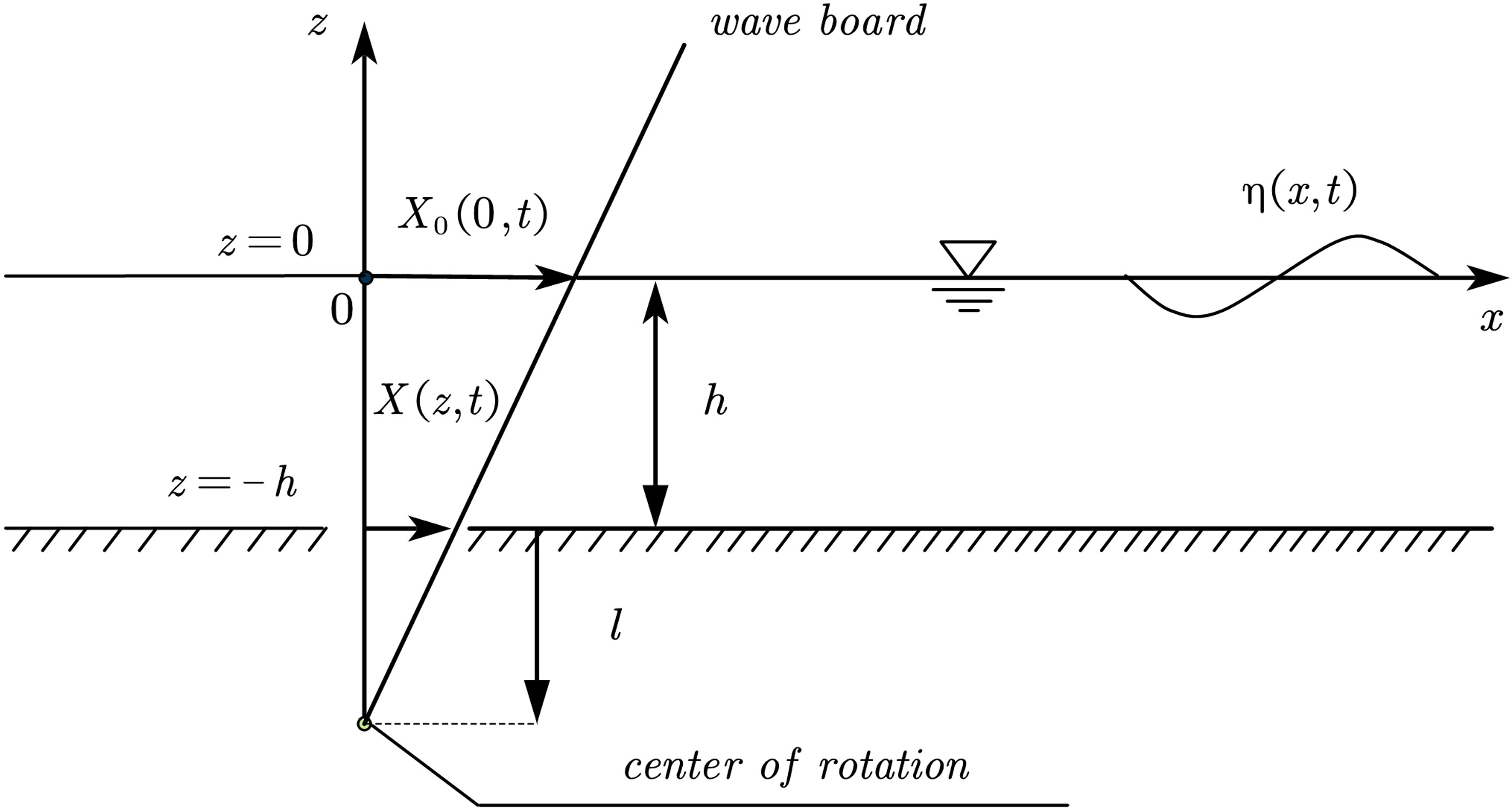
Figure 1 Definition sketch.

Using the Stokes perturbation expansion method, the surface elevation η, the velocity potential Ф, and the wave board position $X_0$ correct to second order expressed with the small ordering parameter $ϵ$ are given by

$$\eta =ϵ{\eta }^{(1)}+{ϵ}^2{\eta }^{(2)}$$

$$\text{Φ}=ϵ{\text{Φ}}^{(1)}+{ϵ}^2{\text{Φ}}^{(2)}$$

$$X_0=ϵX_0^{(1)}+{ϵ}^2{X}_0^{(2)}$$

where the superscript (1) denotes the first-order terms in ($\text{Φ}$, η, $X_0$), that is, (${\text{Φ}}^{(1)}$, ${\eta }^{(1)}$, $X_0^{(1)}$), and the superscript (2) the second-order terms in ($\text{Φ}$, η, $X_0$), that is, (${\text{Φ}}^{(2)}$, ${\eta }^{(2)}$, $X_0^{(2)}$). Employing the above equations, the boundary-value problems for the first- and second-order can be expressed as follows.

The first-order problem

$$\Delta {\text{Φ}}^{(1)}=0$$

$${\text{Φ}}_{tt}^{(1)}+{\text{gΦ}}_z^{(1)}=0\text{ for }z=0$$

$${\text{Φ}}_x^{(1)}=X_{0t}^{(1)}\text{ for }x=0$$

$${\eta }^{(1)}=(1/\text{g}){\text{Φ}}_t^{(1)}\text{\hspace{0.17em}for\hspace{0.17em}}z=0$$

$${\text{Φ}}_z^{(1)}=0\text{\hspace{0.17em}for\hspace{0.17em}}z=-h$$

where g is the gravitational acceleration.

The second-order problem

$$\Delta {\text{Φ}}^{(2)}=0$$

$${\text{Φ}}_{tt}^{(2)}+{\text{gΦ}}_z^{(2)}=-\{{\left[{\text{Φ}}_x^{(1)2}+{\text{Φ}}_z^{(1)2}\right]}_t+{\eta }^{(1)}{\left[{\text{Φ}}_{tt}^{(1)}+{\text{gΦ}}_z^{(1)}\right]}_z\}\text{ for }z=0$$

$${\text{Φ}}_x^{(2)}=-X_0^{(1)}{\text{Φ}}_{xx}^{(1)}+X_{0t}^{(2)}\text{ for }x=0$$

$${\eta }^{(2)}=(1/\text{g})\left({\text{Φ}}_t^{(2)}+(1/2)\left[{\text{Φ}}_x^{(1)2}+{\text{Φ}}_z^{(1)2}\right]+{\eta }^{(1)}{\text{Φ}}_{zt}^{(1)}\right) forz=0$$

$${\text{Φ}}_z^{(2)}=0\text{\hspace{0.17em}for\hspace{0.17em}}z=-h$$

2.1.2 Second-order solution of bichromatic waves

Schäffer (1996) derived the unifying and compact form of the second-order solutions for the motion of the wave board based on the second-order boundary-value problem. In this study, the nonlinear propagation of component waves with the frequencies ω₁ and ω₂ is studied. The wave-maker motion equation of the wave board for bichromatic waves can be obtained by simplifying the detailed forms of the solutions derived by Schäffer (1996)(see the Equations (13) and (42) in (Schäffer, 1996)) as

$$\begin{array}{l}{X}_0(t)=A_1^{*}{\omega }_1\text{cos}({\omega }_{1}t)+A_2^{*}{\omega }_2\text{cos}({\omega }_{2}t)+2B_1^{*}{\omega }_1\text{cos}(2{\omega }_{1}t)\\ + C_2^{*}({\omega }_1-{\omega }_2)\text{cos}[({\omega }_1-{\omega }_2)t]+2B_2^{*}{\omega }_2\text{cos}(2{\omega }_{2}t)\\ + C_1^{*}({\omega }_1+{\omega }_2)\text{cos}[({\omega }_1+{\omega }_2)t]\end{array}$$

where $A_1^{*}$ and $A_2^{*}$ are the amplitudes of the two primary waves, $B_1^{*}$ and $B_2^{*}$ are the amplitudes of the second-order components, and $C_1^{*}$ and $C_2^{*}$ are the amplitudes of the sum and difference frequency components, respectively.

2.2 Numerical model

2.2.1 Numerical wave flume

The bichromatic wave propagation in water with a constant water depth and with a variable topography was simulated in this study.

Figure 2 shows a schematic of the numerical wave flume with a constant water depth and grid meshing of two wave-maker methods. In Figure 2A, the area surrounded by the solid lines denotes the calculation domain when the paddle wave-maker method was employed. Its total length was set as 10 times the maximum wavelength of the two incident waves, and the length of the sponge layer at the right end was set as the maximum wavelength of the two incident waves. s denotes the wave board, θ is the angle between the wave board and the oz-axis, and xoz was used as coordinate system. The calculation domain for the modified mass source method consisted of the calculation domain for the paddle wave-maker method and the added area which was surrounded by the dashed lines shown in Figure 2A. A sponge layer was set at the left end in the added area. s₁ and s₂ denote the first and second sources, respectively.

Figure 2

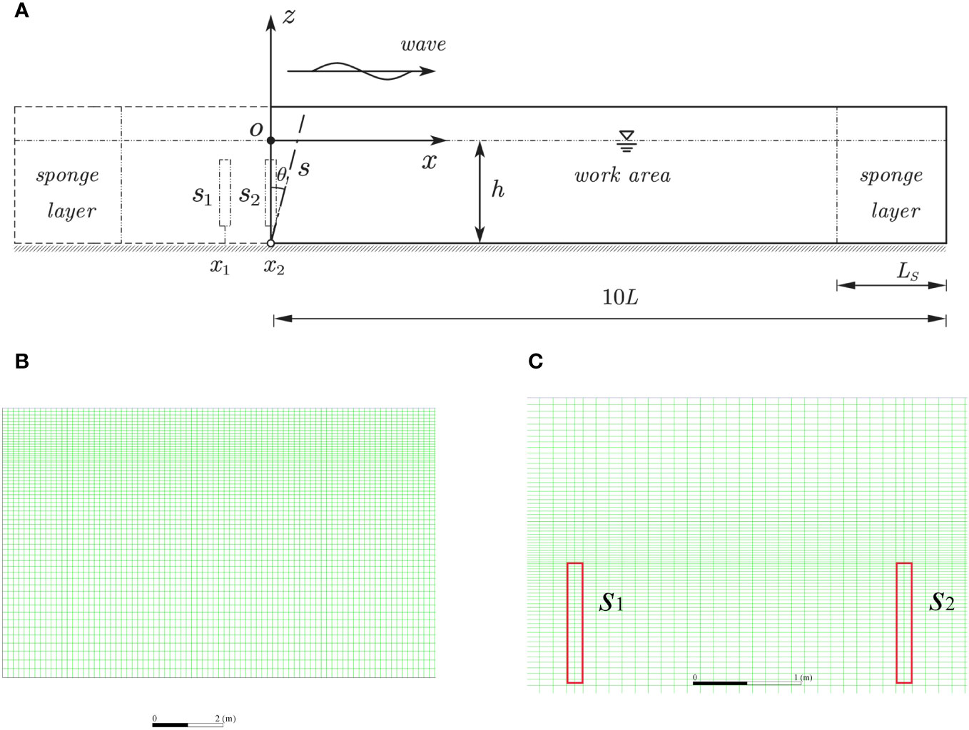
Figure 2 Sketch of numerical wave flume with a constant water depth and grid meshing of two wave-maker methods [(A) numerical wave flume; (B) grid meshing of wave board method; (C) grid meshing of mass source method].

Figure 3 shows a sketch of the numerical wave flume with a variable topography bottom for the paddle wave-maker method. The topography of the wave flume in a physical experiment (Xu et al., 2009) is simplified to obtain a numerical wave flume with a variable topography bottom here because the effects of current on the non-linearity of the wave are not considered in this study. The still depth was 0.5 m in the deep region and decreased to 0.25 m at the top of the bar, which consisted of a 1:20 upward slope, a 1:60 upward slope, a 6 m horizontal crest, a 1:40 downward slope, and a 1:10 downward slope. A wave sponge layer with the uniform length of 2.0 m was set at the right end. When the modified mass source wave-maker method was adopted, the first part of the wave flume was the same as the added area which is surrounded by the dashed lines in Figure 2A, while the second part was the same as that shown in Figure 3.

Figure 3

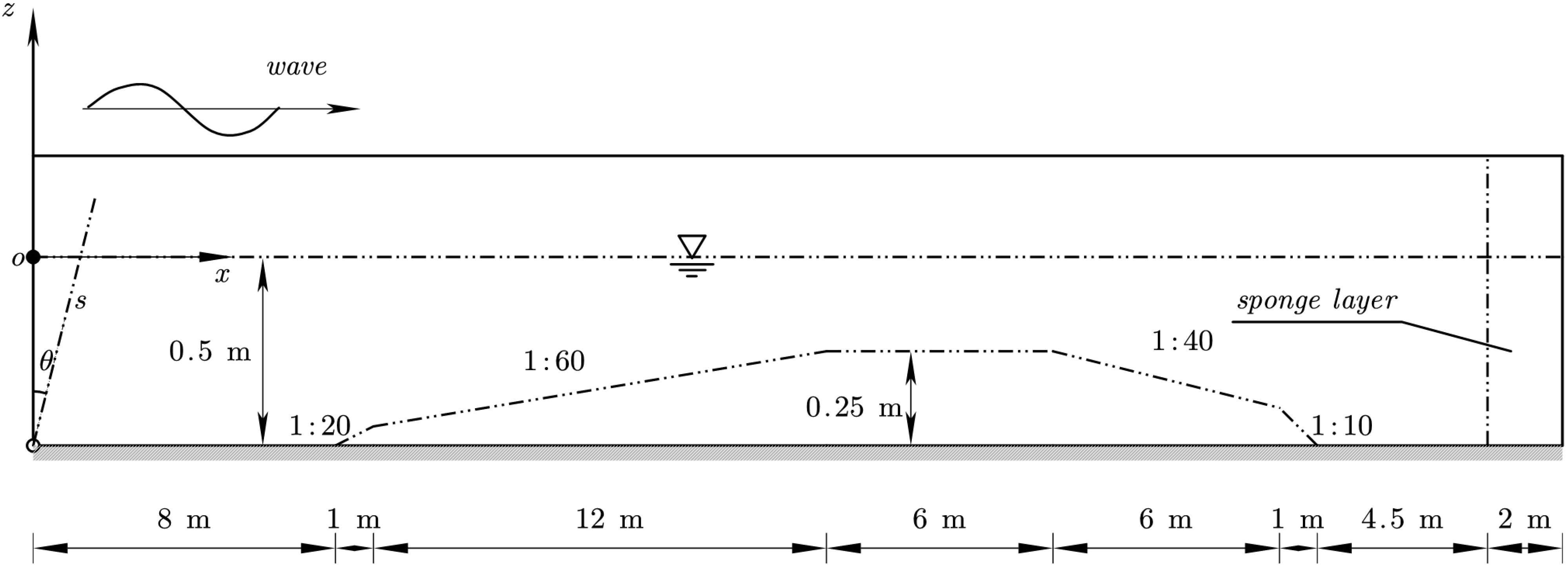
Figure 3 Sketch of the numerical wave flume with a variable topography bottom for the paddle wave-maker method.

The modified mass source wave-maker method was described in detail in Subsection 2.2.2. The grid meshing of two wave-maker methods for specific cases was described in detail in Subsections 2.3.1 and 2.4.1.

2.2.2 The modified mass source wave-maker method

The numerical results from the paddle wave-maker method were compared with those from the modified mass source wave-maker method presented by Chen et al. (2021), who adopted two wave sources to generate bichromatic waves. As shown in Figure 2A, x_i (i =1, 2) is the horizontal coordinate of the center point of wave-maker region Ω. The horizontal coordinate of the center point for the second source, x_2, equates 0, and that for the first source is taken as x₁. The functions for the two mass sources are expressed as

$$S_{m1}=\frac{2c_1{a}_1}{A_{\text{Ω}}}\text{cos}(k_1{x}_1-{\omega }_{1}t)$$

$$S_{m2}(t)=\frac{2c_2{a}_2}{A_{\text{Ω}}}\text{cos}(-{\omega }_{2}t)$$

where, a₁ and a₂ are the amplitudes of the two incident waves, k₁ is the wave number of the first incident wave, c₁ and c₂ are the wave velocities of the two incident waves, A_Ω is the total area of the grid covered by the wave-maker region. S_m1 and S_m2 are the mass source functions of s₁ and s₂, respectively.

2.2.3 Relevant setup of Fluent

The k-epsilon model and pressure implicit with splitting of operators (PISO) algorithm in the Fluent software were used for the numerical simulation in this study. It is necessary to perform secondary development at the locations of the wave-maker and sponge layer in the Fluent software to establish the numerical flume model for wave propagation. The expression for the second-order motion equation of the wave board and the functions for the two wave sources were programmed and the source term in the governing equation was defined to realize wave generation and wave absorption. When the paddle wave-maker method was adopted, the left boundary of the wave flume was set as the moving boundary, and a moving grid was used to realize the numerical wave generation. When the modified mass source wave-maker method was employed, the left boundary of the wave flume was set as the sponge layer to realize the numerical wave absorption. For both two wave-maker methods, the right boundary of the wave flume was set as the sponge layer. The effect of the sponge layer is related to its width, which is often set to 1−2 times the incident wavelength. In this study, a momentum source is added to the momentum equation to absorb the wave. The absorbing source terms are given by

$$S_x=-\rho \xi (x)u$$

$$S_z=-\rho \xi (x)w$$

$$\xi (x)=\alpha (x-x_{sl})/(x_{sr}-x_{sl})$$

where $S_x$ and $S_z$ are the additional momentum source terms in the x and z directions, respectively; $u$ and $w$ are the velocity variables of the water particles in the x and z directions, respectively; $\alpha$ is the damping coefficient, which is taken as 6.0, and $x_{sl}$ and $x_{sr}$ are the horizontal coordinates of the start and end points of the sponge layer, respectively.

2.3 Numerical simulation and verification of bichromatic waves in waters of uniform depth

2.3.1 Parameter settings and grid meshing

The amplitudes of each component of the incident bichromatic waves were all set as 0.01 m, and different wave periods were used in the different combinations. Table 1 lists the parameters of the incident waves in the studied cases. In Table 1, T, L, and μ (μ = h/L) denote the period, wavelength, and ratio of water depth to the wavelength, respectively. Case A1 considers the bichromatic wave combination of two transition water waves, and Case A2 considers the bichromatic wave combination of a transition water wave and a shallow-water wave. Cases B1 and B2 consider the combination of a deep-water wave and a transition water wave. The water depths for cases A1 and A2 were both set as 0.45 m and those for Cases B1 and B2 were both set as 4.0 m. The frequencies of the two incident waves were f₁ and f₂, respectively. The nonlinear interactions between the waves lead to the sum frequency, difference frequency, and higher harmonic components.

Table 1

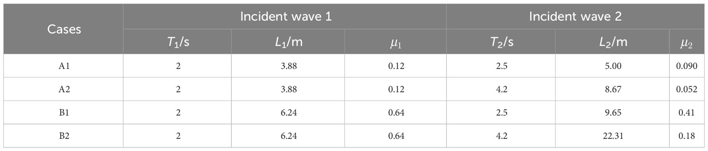
Table 1 Table of parameters for different combinations of incident waves.

The wave flume in Figure 2A was used for grid meshing. As shown in Figure 2B, when the paddle wave-maker method was adopted, a structured grid was used in the work area. We have conducted a lot of tests to simulate the propagation of bichromatic waves with different grid sizes and time steps and finally selected the parameters as follows. The grid size in the horizontal direction, Δx, was set to 1/35 of the maximum wavelength of the two incident waves. Δx was non-uniform in the sponge layer, and increased gradually with a ratio of 1.06 along the wave propagation direction. The grid size in the vertical direction, Δz, was taken as 1/10 of the wave height of the two incident waves within a distance of one wave height away from the still water level, and increased gradually towards the bottom and top of the wave flume with a ratio of 1.03 in the remaining area. The time step, Δt, was set as 0.005 s, and the number of iterations for each time step was set as 20.

As shown in Figure 2C, when the modified mass source wave-maker method was employed, the two wave sources were set to the same size. The width and height of the wave sources for Cases A1 and A2 were 0.2 m and 0.44 m, respectively, and the center of the wave source region was located at 0.5 times the water depth beneath the still water level. The left end of s₁ was located 5.0 m away from the right end of the sponge layer in the front segment of the wave flume, and s₂ was located at the right side of s₁. The horizontal distance between the two wave source centers was 2.0 m. Δx was set as 0.05 m, Δz as 0.01 m, and Δt as 0.01 s. The width and height of the two wave sources for Cases B1 and B2 were 0.1 m and 0.74 m, respectively, and the top of the wave source region was set as the value of the wave height away from the still water level. The other parameters for the two wave sources were the same as those for Cases A1 and A2. In the work area, Δx was set as 0.05 m near the two wave sources, and as 0.08 m in the remaining region. For all the cases, a non-uniform grid was adopted in the horizontal direction in the sponge layer similar to the grid adopted when the paddle wave-maker method was employed; a non-uniform grid was also employed in the vertical direction. Δz was set as 0.025 m near the still water level and gradually increased with the water depth to 0.18 m at the bottom of the wave flume. Δt was also set as 0.01 s.

2.4 Numerical simulation and verification in the wave flume with an uneven bottom

2.4.1 Grid division

The wave flume in Figure 3 was used for grid meshing. Similar to Figure 2B, when the paddle wave-maker method was adopted, a structured grid was also adopted in the work area. Δx was set to 1/40 of the maximum wavelength of the two incident waves. Similar to subsection 2.3, a non-uniform grid was adopted along the horizontal direction of the sponge layer. To capture the variation of the wave profile efficiently, the grid along the vertical direction within a wave height of the still water level was more refined and contained 15 grid nodes. Outside this area, the grid gradually became coarser towards the bottom and top of the wave flume at a ratio of 1.03. Δt was set as 0.005 s, and the number of iterations for each time step was 20.

Similar to Figure 2C, the width and height of the two wave sources were set as 0.09 m and 0.25 m, respectively, and the distance between the top of the wave source and the still water level was set as 0.1m. The distance between the left side of s₁ and the right end of the sponge layer in the front part of the wave flume was 5.0 m, s₂ was located at the right side of s₁, and the horizontal distance between the two wave source centers was 2.0 m. Δx was set as 0.045 m near the wave sources in the work area, and as 0.08 m in the remaining domain. A non-uniform grid similar to that described in subsection 2.3 was adopted in the horizontal direction in the sponge layer. A non-uniform grid was also adopted in the vertical direction. The grid within a wave height of the still level was more refined and had 12 grid nodes, while Δz was set as 0.05 m in the remaining region. An unstructured grid was set near the submerged bar. Δt was taken as 0.01 s.

2.4.2 Test cases

The two wave-maker methods were adopted to simulate the generation of bichromatic waves, and the calculation results were compared with the experimental data (Xu et al., 2009).

Table 2 lists the incident wave parameters for the different cases. In Table 2, ${\mu }^{*}$ (${\mu }_1^{*}$ and ${\mu }_2^{*}$) denotes the ratio of the water depth in the deeper region to L. f_g is the difference (f_g = f₁–f₂) between the two primary frequencies, that is, the frequency of the wave groups. The ratio of the amplitudes of the two primary waves (δ = a₂/a₁) is called the modulation rate of the wave groups (Baldock et al., 2000). When a₁ = a₂, the wave groups are fully modulated wave groups. To study the effects of the wave group frequency and the incident wave parameters on the propagation of bichromatic waves, the test cases were divided into the four groups F, H, S, and W. The amplitudes of the two primary waves in group F, which includes the three Cases F1, F2, and F3, were all set as 0.0175 m. The wave groups were therefore fully modulated wave groups, and the effects of different f_g on the propagation of the bichromatic waves were studied. Group H includes the three Cases H1, H2, and H3, and all of which had the same frequencies in order to study the effects of different incident wave amplitudes on the nonlinearity of the bichromatic wave propagation. Group S considers a strongly modulated wave group (δ = 0.8), and group W a weakly modulated wave group (δ = 0.2). The sum of the amplitudes in the two groups S and W was equal to 0.045 m. The effect of the modulation rates on the propagation of bichromatic waves can be studied by comparing the results for groups F, S, and W. For all test cases, the wave at the crest of the submerged bar is a transition wave, and wave breaking does not appear during propagation.

Table 2

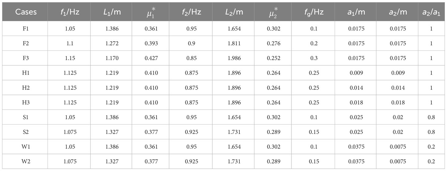
Table 2 Table of incident wave parameters.

3 Results

3.1 Calculation results and analyses of numerical simulation of bichromatic waves in waters of uniform depth

The second-order approximate solutions for the nonlinear interaction of gravitational surface waves derived by Hong (1980) based on the Stokes finite amplitude wave theory and the perturbation method [see the Equations (2-2) and (2-6) in (Hong, 1980)] were used as the theoretical solutions for comparison.

Figures 4, 5 show the comparisons between the results from the two numerical models and the theoretical solutions for Cases A1 and A2, respectively. From Figure 4, it can be seen that the results obtained from the modified mass source wave-maker method are in good agreement with the theoretical solutions, while the results obtained from the paddle wave-maker method are slightly larger than those from the theoretical solutions. As shown in Figure 5, there is a large difference between the results calculated using the paddle wave-maker method and those calculated using the modified mass source wave-maker method as well as the theoretical solutions. The amplitude calculated using the paddle wave-maker method is larger and the waveform is different. This is because incident wave 2 in Case A2 is a shallow-water wave, while the numerical paddle wave-maker method is derived based on the Stokes wave theory and is therefore not applicable to shallow-water waves. In addition, we calculated several cases in which the period of incident wave 2 varied from 2.5 s to 4.2 s, and found that the paddle wave-maker method was not applicable when ${\mu }_2<0.065$.

Figure 4

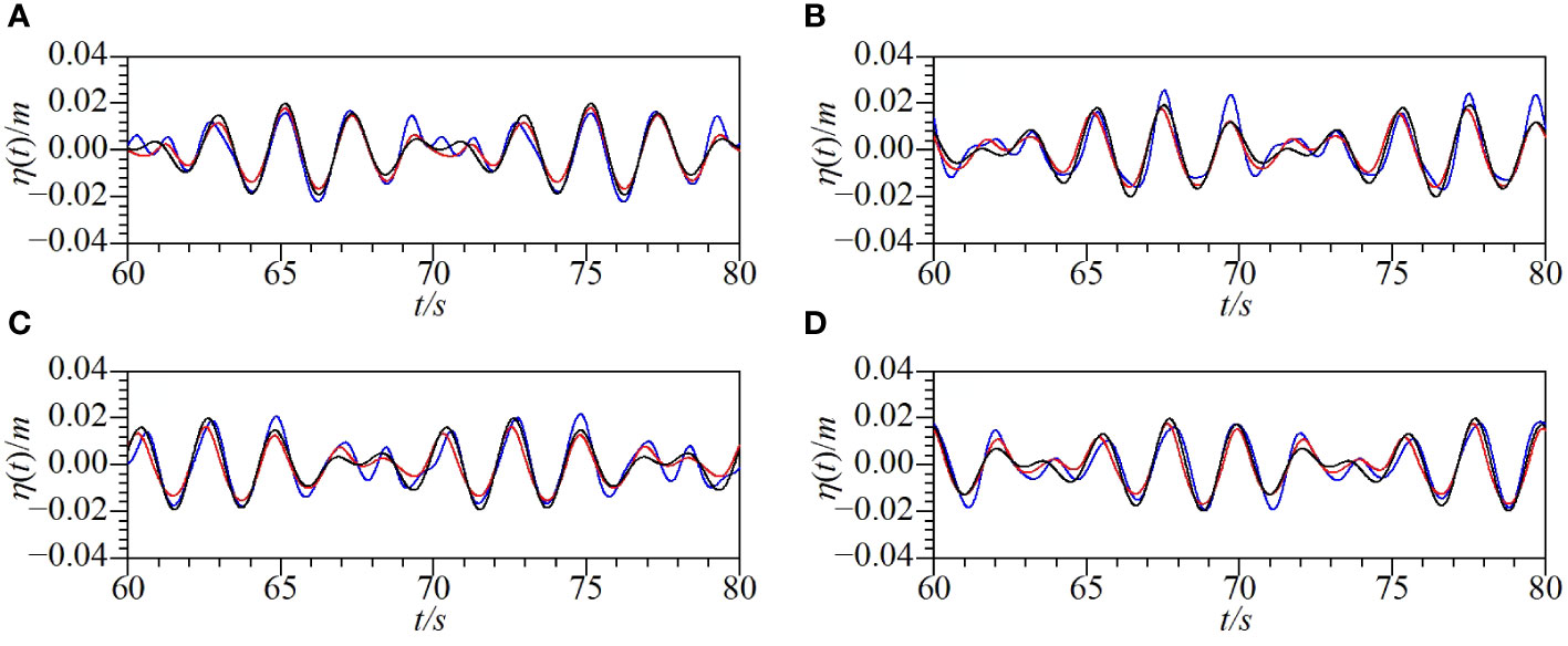
Figure 4 Comparisons of the time series of surface displacements at different locations for Case A1 (solid black line: theoretical solution; solid red line: numerical solution from mass source method; solid blue line: numerical solution from wave board method) [(A) x=2.5L₂; (B) x=5L₂; (C) x=7.5L₂; (D) x=10L₂].

Figure 5

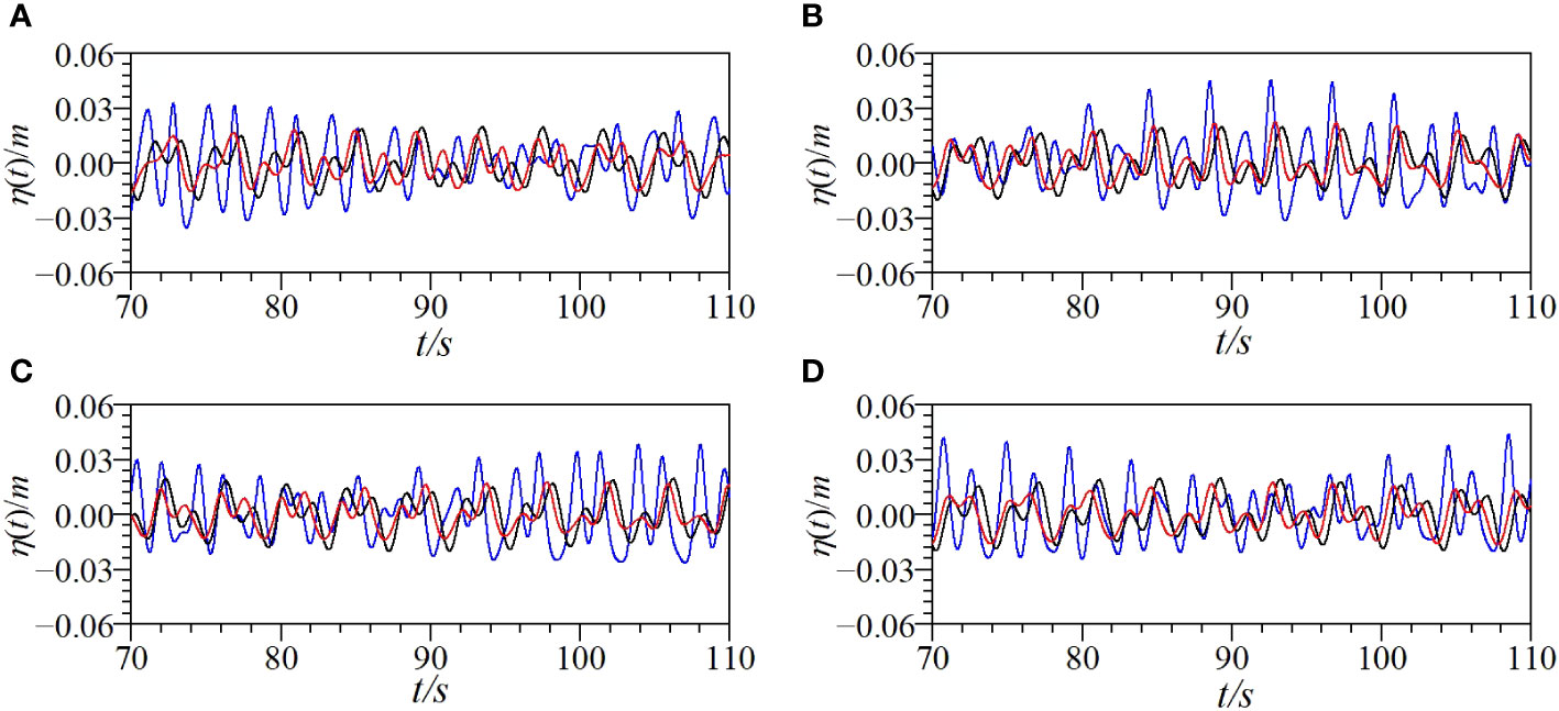
Figure 5 Comparisons of the time series of surface displacements at different locations for Case A2 (solid black line: theoretical solution; solid red line: numerical solution from mass source method; solid blue line: numerical solution from wave board method) [(A) x=2.5L₂; (B) x=5L₂; (C) x=7.5L₂; (D) x=10L₂].

Figures 6, 7 show the comparisons between the results from the two numerical models and the theoretical solutions for Cases B1 and B2, respectively. As shown in Figures 6, 7, the results from the two numerical models are basically consistent with the theoretical solution. Comparing Figures 6A–D to Figures 7A–D, it can be observed that for the cases considered and the grid adopted, the attenuation of the wave amplitude along the wave flume calculated using the paddle wave-maker method is almost zero, and the same waveform at the beginning is still maintained at $x=10L$ without any attenuation. However, the results from the modified mass source wave-maker method compared to the theoretical solutions attenuate by 15% or so. Therefore, the results from the paddle wave-maker method are in better agreement with the theoretical solutions than those from the modified mass source wave-maker method.

Figure 6

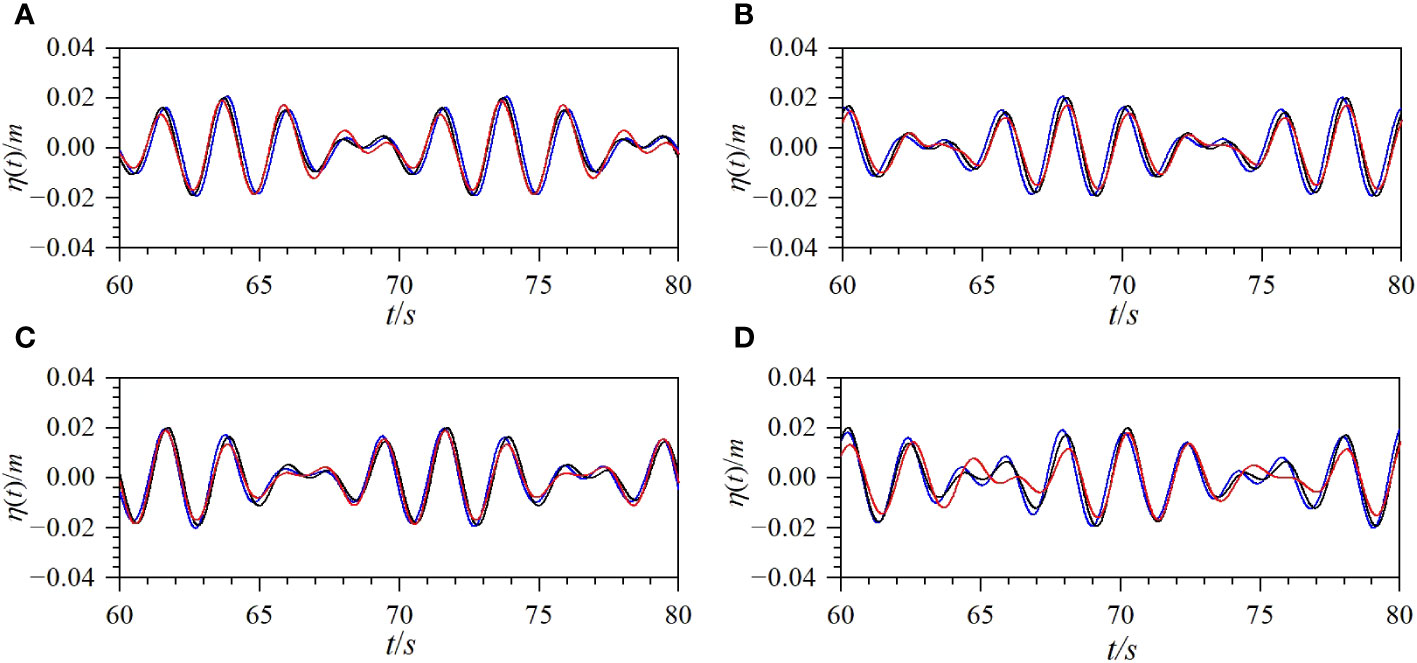
Figure 6 Comparisons of the time series of surface displacements at different locations for Case B1 (solid black line: theoretical solution; solid red line: numerical solution from mass source method; solid blue line: numerical solution from wave board method) [(A) x=2.5L₂; (B) x=5L₂; (C) x=7.5L₂; (D) x=10L₂].

Figure 7

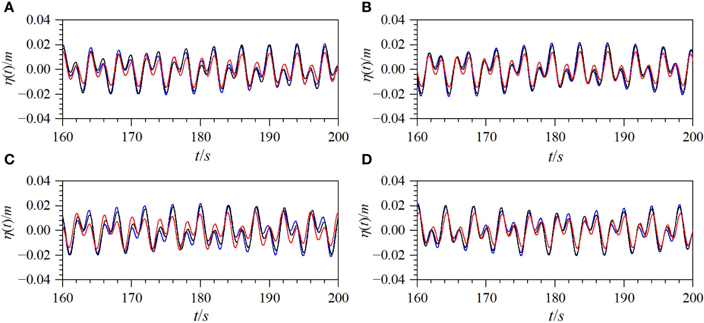
Figure 7 Comparisons of the time series of surface displacements at different locations for Case B2 (solid black line: theoretical solution; solid red line: numerical solution from mass source method; solid blue line: numerical solution from wave board method) [(A) x=2.5L₂; (B) x=5L₂; (C) x=7.5L₂; (D) x=10L₂].

The interactions between different wave components in the bichromatic wave field are then analysed through spectral analysis; that is, the frequency components are obtained through the Fourier transformation of the time-domain wave profile data at different locations. Figure 8 shows the spatial distribution of the amplitude of each frequency component in Cases A1, A2, B1, and B2. From Figures 8A–D, it can be observed that the differences between the numerical results and the theoretical solutions for Case A2 are more obvious than those for Case A1, also indicated in Figures 4, 5. This is because Case A2 is the bichromatic wave combinations of a transition water wave and a shallow-water wave, instead, Case A1 is the bichromatic wave combinations of two transition water waves. The nonlinearity in Cases A1 and A2 can both be illustrated adequately by the numerical results. From Figures 8E–H, it can be observed that, for Cases B1 and B2, the numerical results are basically consistent with the theoretical solutions, also indicated in Figures 6, 7. This is because Cases B1 and B2 are the bichromatic wave combinations of a deep-water wave and a transition water wave, and the nonlinearity is not significant for the two cases. Case B1 is used as an example to illustrate the harmonics of the bichromatic wave field obtained using the paddle wave-maker method. Figure 8E shows that the amplitudes of the two primary frequencies, f₁ and f₂, are both 0.01 m and do not change along the wave flume. Figure 8F show that, the difference frequency components, f₁–f₂, and second-order components, 2f₁, f₁ + f₂, and 2f₂, are basically zero along the wave flume, which indicates that the wave field in this case has weak nonlinearity and that little energy is transferred from the low-order frequency components to the high-order frequency components.

Figure 8

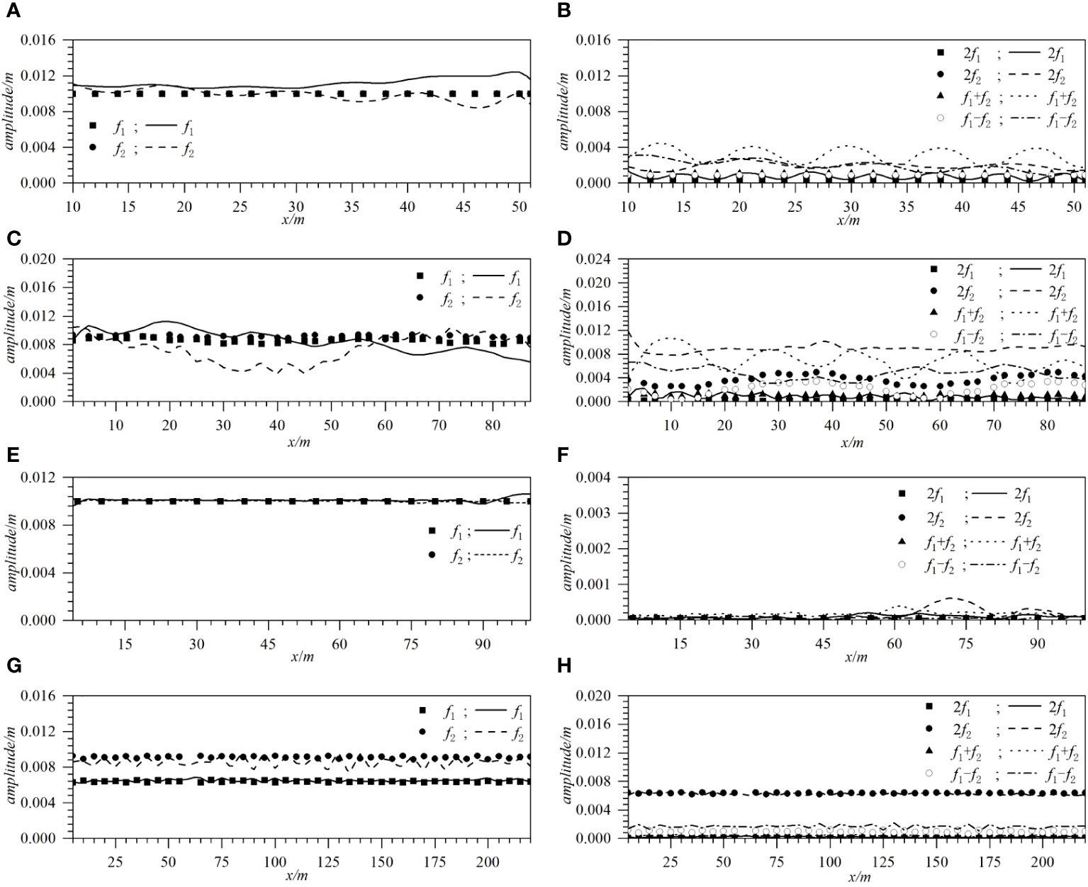
Figure 8 Comparisons of the spatial variation of amplitudes of each frequency component for Cases A1, A2, B1, and B2 (solid line, dashed line, dotted line, dashed-dotted line: numerical solutions from wave board method; blacksquare, blackcircle, blacktriangle, circle: theoretical solutions) [(A) f₁ and f₂ for Case A1; (B) 2f₁, 2f₂, f₁+f₂, and f₁-f₂ for Case A1; (C) f₁ and f₂ for Case A2; (D) 2f₁, 2f₂, f₁+f₂, and f₁-f₂ for Case A2; (E) f₁ and f₂ for Case B1; (F) 2f₁, 2f₂, f₁+f₂, and f₁-f₂ for Case B1; (G) f₁ and f₂ for Case B2; (H) 2f₁, 2f₂, f₁+f₂, and f₁-f₂ for Case B2].

3.2 Calculation results and analyses of numerical simulation of bichromatic waves in waters with an uneven bottom

Taking Case F1 as an example, the propagation of bichromatic waves was simulated using the two numerical models. Case F1 considers the bichromatic wave combination of 1.05 Hz and 0.95 Hz. Figure 9 compares the time series of the surface displacements and the upper wave envelopes calculated with the two numerical models and those of the experimental data. As shown in Figure 9, the results from the two numerical models are basically consistent with the experimental data. The calculated waveforms are stable, and the amplitude of the bichromatic waves (approximately 0.035 m) is approximately twice that of the primary wave (0.0175 m). By carefully observing the calculated upper wave envelope and the experimental data shown in Figure 9, it can be found that with the calculation grid adopted in this study, the upper wave envelope calculated by the paddle wave-maker method is closer to the experimental data. Therefore, the paddle wave-maker method provides better results than the modified mass source wave-maker method. Figure 10 shows the comparisons of the numerical solutions and the experimental data for the amplitude spectrum of each harmonic component at different locations for Case F1. As shown in Figure 10, owing to the nonlinear interactions of the bichromatic waves, higher-order harmonics with obvious amplitudes are generated. The amplitudes of the two primary waves, which have the frequencies of f₁ and f₂, respectively, decrease as the propagation distance increases. The energy in the wave field is redistributed owing to the nonlinear effects of the waves. The energy of the low-frequency wave components is gradually transferred to the high-frequency harmonics, which leads to an increase in the amplitudes of the high-frequency harmonics. As shown in Figure 10, the amplitude of each frequency component calculated by the paddle wave-maker method is closer to the experimental data, which is also indicated in Figure 9.

Figure 9

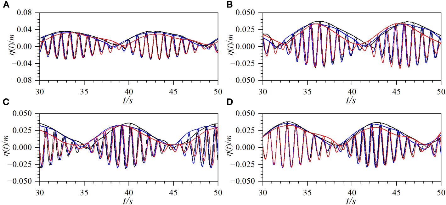
Figure 9 Comparisons of time series of surface displacement and upper envelope of wave profile at different locations for Case F1 (solid black line: experimental data; solid blue line: numerical solutions from wave board method; solid red line: numerical solutions from mass source method) [(A) x=6 m; (B) x=13 m; (C) x=23 m; (D) x=35 m].

Figure 10

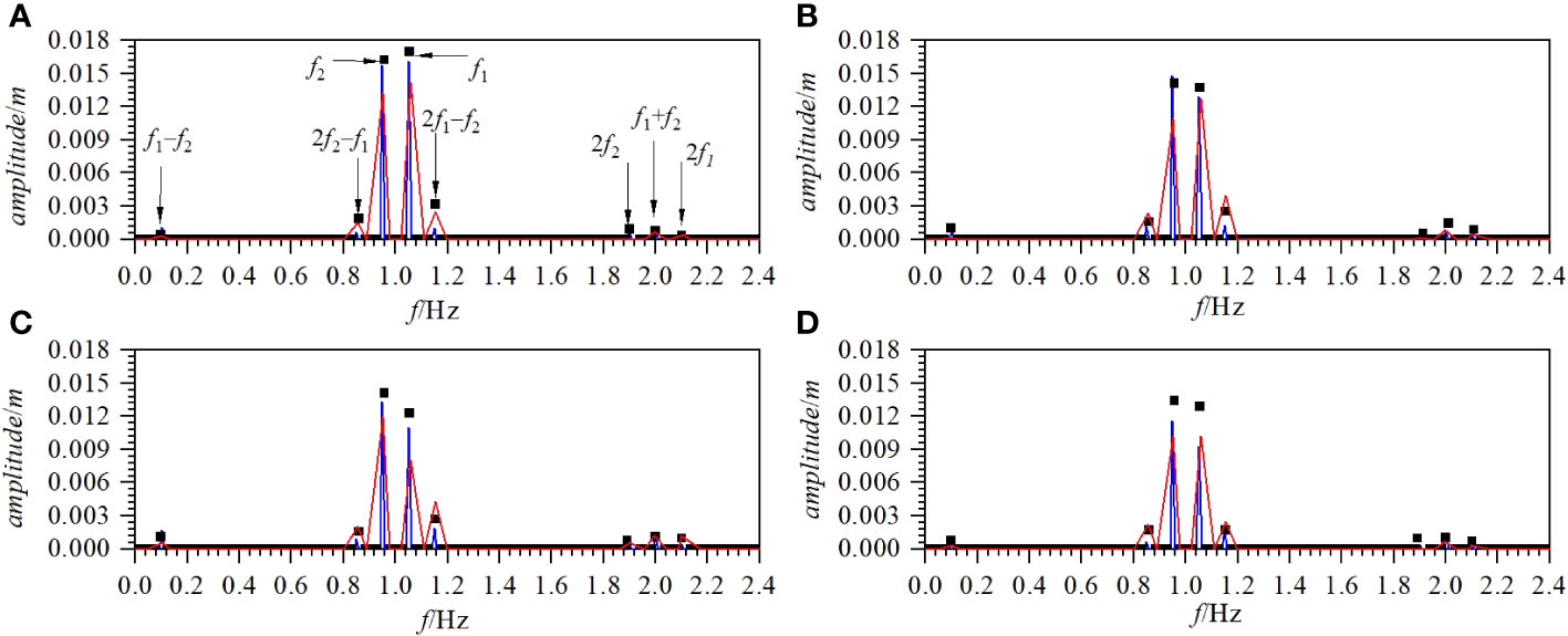
Figure 10 Comparisons of the spatial variation of amplitudes of each frequency component for Case F1 (blacksquare: experimental data; solid blue line: numerical solutions from wave board method; solid red line: numerical solutions from mass source method) [(A) x=6 m; (B) x=13 m; (C) x=23 m; (D) x=35 m].

To analyze the effects of the wave group frequency on the nonlinear interactions of the bichromatic wave field, the time series of the surface displacement and upper envelope of the wave profile calculated with the two numerical models for the two cases of group F (F2 and F3) at x = 6.0 m are compared with the experimental data, as shown in Figure 11. As shown in Table 2, the wave group frequencies of F1, F2, and F3 are 0.1, 0.2 and 0.3, respectively. As shown in Figures 9A, 11, as the frequency of the wave group increases, the wave crest of the upper envelope of the wave profile of the bichromatic waves becomes steeper, the main peak in the waveform becomes sharper. The agreement between the numerical solutions from the paddle wave-maker method and the experimental data is slightly better than that of the mass source wave-maker method.

Figure 11

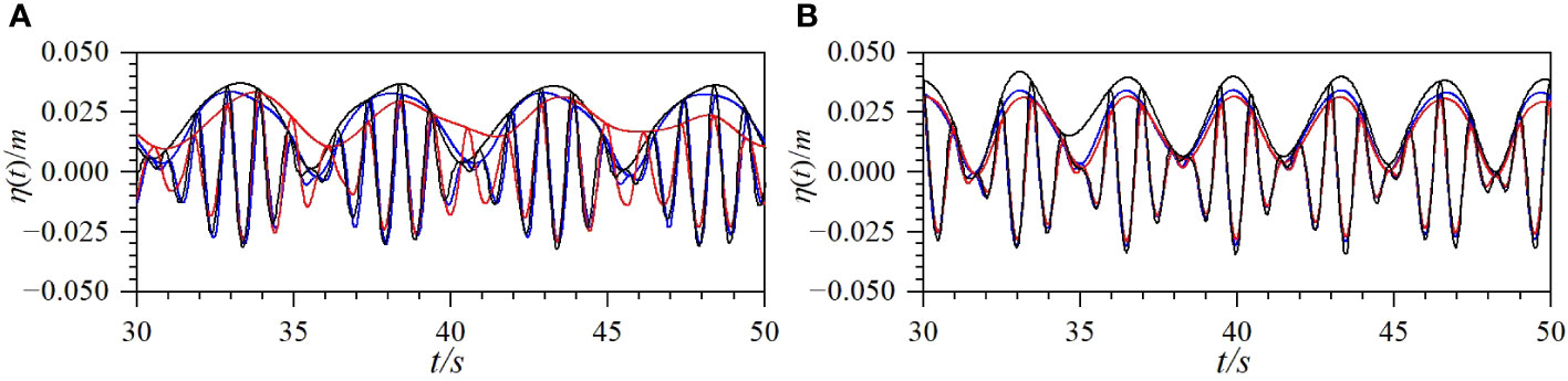
Figure 11 Comparisons of time series of surface displacements and upper envelope of wave profile for group F (F2, F3) at x = 6 m (solid black line: experimental data; solid blue line: numerical solutions from wave board method; solid red line: numerical solutions from mass source method) [(A) Case F2; (B) Case F3].

To study the effects of wave amplitude on bichromatic waves, different amplitudes of primary waves were set for the cases in Group H; the amplitudes increase successively from Cases H1 to H3. Figure 12 shows the comparisons of the time series of the surface displacement and the upper envelope of the wave profile for the cases in group H at x = 6.0 m obtained from the two numerical models with those from the experimental data. As shown in Figure 12, the results from the two numerical models are consistent with the experimental data. It can be observed from Figure 12 that the numerical results from the paddle wave-maker method are still slightly better than those from the mass source wave-maker method. As shown in Figure 12, as the amplitude of the incident wave increases, the amplitude of the bichromatic waves also increases.

Figure 12

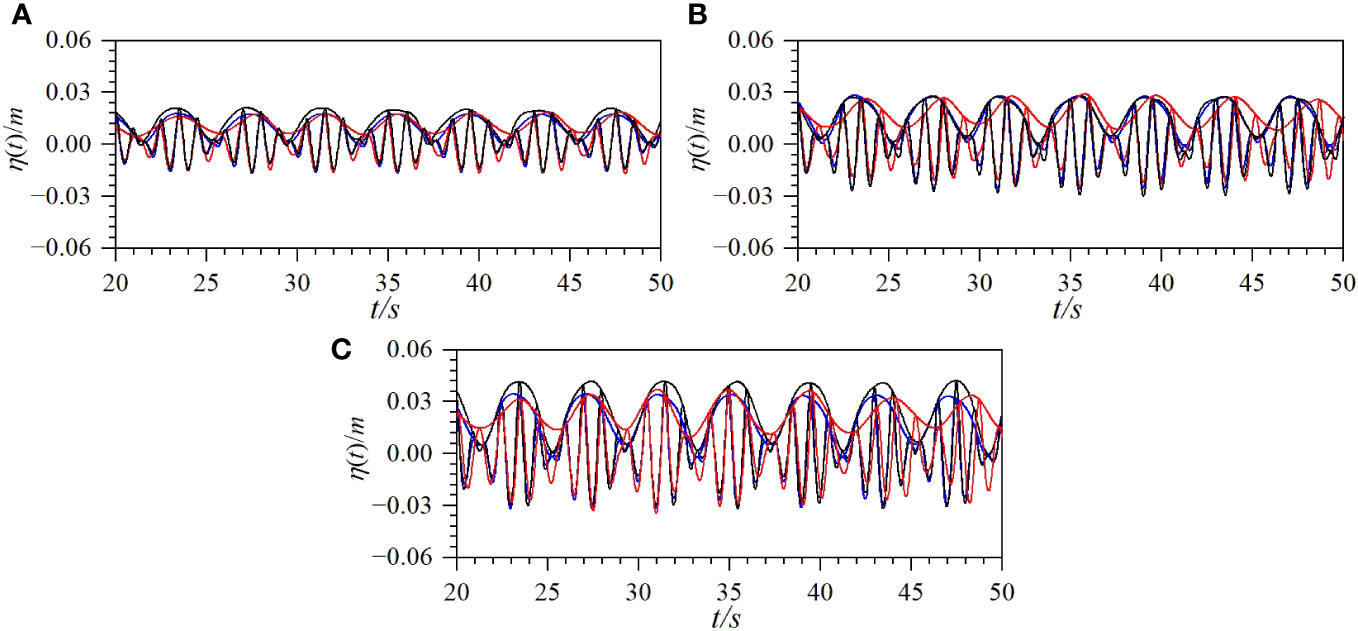
Figure 12 Comparisons of time series of surface displacement and upper envelope of wave profile for group H at x = 6 m (solid black line: experimental data; solid blue line: numerical solutions from wave board method; solid red line: numerical solutions from mass source method) [(A) Case H1; (B) Case H2; (C) Case H3].

The modulation rate is an important parameter of bichromatic waves (Baldock et al., 2000). Figure 13 shows the comparisons of the time series of the surface displacement and upper envelope of the wave profile for the cases of S1 and W1 at x = 6.0 m obtained from the two numerical models to the experimental data. Comparing Figure 9A with Figure 13A, it can be seen that the waveform basically does not change as the modulation rate decreases from that of the fully modulated wave group to that of the strongly modulated wave group. Comparing Figures 13A, B, it can be observed that, as the modulation rate decreases from that of strongly modulated wave group to that of the weakly modulated wave group, the amplitude of the upper envelope of the wave profile becomes smaller, and the waveform becomes more regular and symmetrical. At the same time, the main peak in the wave envelope becomes gentler. For bichromatic wave groups with different modulation rates, the results from the paddle wave-maker method agree better with the experimental data than those from the mass source wave-maker method.

Figure 13

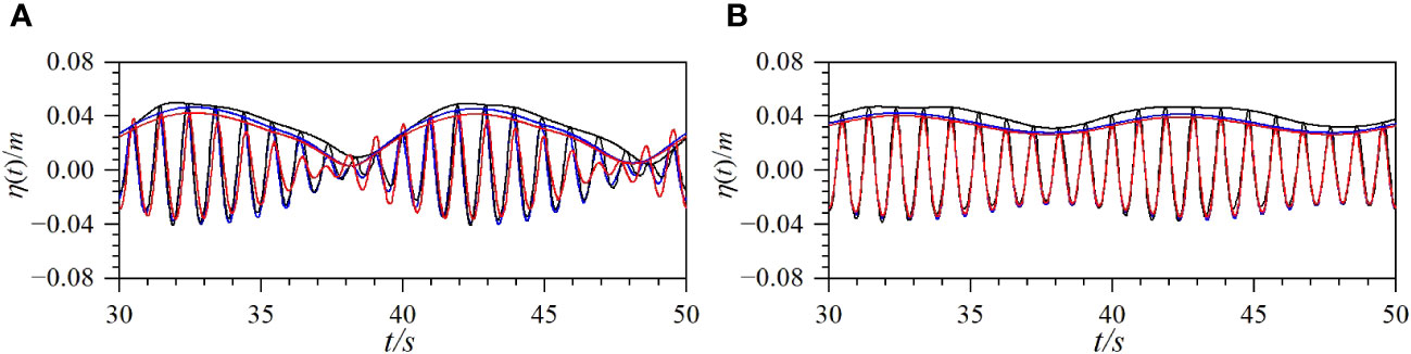
Figure 13 Comparisons of time series of surface displacement and upper envelope of wave profile for the Cases (S1, W1) at x = 6 m with different modulation rates (solid black line: experimental data; solid blue line: numerical solutions from wave board method; solid red line: numerical solutions from mass source method) [(A) Case S1; (B) Case W1].

4 Discussion and conclusions

The wave-maker theory proposed by Schäffer (1996) has been widely used in physical experiments. Dong et al. (2022) used the second-order wave-maker theory proposed by Schäffer (1996) to suppress the generation of spurious free-wave and obtained accurate and stable wave signals when studying the low-frequency harbor oscillations. When Ma et al. (2022) studied freak waves, they proposed a modified time reversal method using a second-order transfer function proposed by Schäffer (1996) as the first step of the correction procedure to reconstruct some in-situ measured waves. Díaz-Carrasco et al. (2021) proposed an improved formula to estimate the reflection coefficient for the rubble mound breakwaters, and they used the wave-maker theory of Schäffer (1996) to create second-order irregular waves. Schaffer’s method was rarely combined with FLUENT software in numerical simulations. Researchers used the wave-maker theory proposed by Schäffer (1996) more to study specific problems, and the water depth applicable range of the wave-maker method based on this theory has not been discussed in detail. The mass source wave-maker method is a relatively mature method in numerical simulation (Peric and Abdel-Maksoud, 2015; Bai et al., 2020). At present, no researchers have compared the applicability of the second-order paddle wave-maker method and the mass source wave-maker method in numerical simulation.

In this study, the second-order wave-maker theory proposed by Schäffer (1996) for physical experiments was combined with the Fluent software to effectively simulate the propagation of nonlinear water waves. By using the secondary development function in the Fluent software, and a dynamic mesh, the second-order paddle wave-maker numerical wave-maker was realized using the pseudo-physical wave-maker method. To discuss the specific applicable scopes of water depth for different wave maker methods, the results for the propagation of bichromatic waves in a numerical wave flume with uniform and non-uniform depths obtained from the paddle wave-maker method were detailed compared with those from the modified mass source method. The paddle wave-maker method is not suitable for bichromatic wave combinations containing shallow-water waves, especially when ${\mu }_2<0.065$. For the bichromatic wave combination of two transition water waves, and the combination of a transition water wave, and a deep-water wave, the calculation results from the paddle wave-maker method are superior to those from the mass source wave-maker method, at least for the grid divisions adopted in this study.

Through the frequency spectrum analysis, it was found that the energy in the wave field is transferred from the low-frequency components to the high-frequency components as bichromatic waves propagate in a flume with a variable topography bottom. This process becomes more obvious when the nonlinear effects between wave components become larger, and the energy in the wave field becomes more dispersed. Additionally, the relationships between the incident wave parameters and wave-wave nonlinear interactions were also investigated in this study. Through the numerical simulation of several different cases and comparison of the calculated results with the experimental data, it was found that increasing the amplitudes of the incident waves can cause the amplitudes of the wave group to increase correspondingly. Varying the wave group frequency has a direct impact on the waveform of the wave envelope. A higher wave group frequency results in a steeper crest of the upper envelope of the wave profile.

Data availability statement

The raw data supporting the conclusions of this article will be made available by the authors, without undue reservation.

Author contributions

Z-HZ: Data curation, Formal analysis, Methodology, Software, Validation, Visualization, Writing – original draft, Writing – review & editing. H-SZ: Conceptualization, Funding acquisition, Methodology, Supervision, Writing – review & editing. P-BZ: Data curation, Formal analysis, Investigation, Software, Writing – review & editing. M-YC: Investigation, Resources, Software, Validation, Writing – review & editing.

Funding

The author(s) declare financial support was received for the research, authorship, and/or publication of this article. This work was supported by the National Natural Science Foundation of China (Grant Nos. 51679132 and U22A20216), the Science and Technology Commission of Shanghai Municipality (Grant No. 21ZR1427000), and Shanghai Frontiers Science Center of “Full Penetration” Far-Reaching Offshore Ocean Energy and Power.

Conflict of interest

The authors declare that the research was conducted in the absence of any commercial or financial relationships that could be construed as a potential conflict of interest.

Publisher’s note

All claims expressed in this article are solely those of the authors and do not necessarily represent those of their affiliated organizations, or those of the publisher, the editors and the reviewers. Any product that may be evaluated in this article, or claim that may be made by its manufacturer, is not guaranteed or endorsed by the publisher.

References

Bai X. D., Zhang W., Zheng J. H., Wang Y. (2020). On the mass source internal wave making method for ALE based numerical wave tank. J. Mar. Sci. TECH 25 (4), 1093–1102. doi: 10.1007/s00773-020-00702-z

CrossRef Full Text | Google Scholar

Baldock T. E., Huntley D. A., Bird P., O’hare T., Bullock G. N. (2000). Breakpoint generated surf beat induced by bichromatic wave groups. Coast. Eng. 39 (2), 213–242. doi: 10.1016/S0378-3839(99)00061-7

CrossRef Full Text | Google Scholar

Chen M.-Y., Zhang H.-S., Zhou E.-X., Xu D.-L. (2021). Numerical bichromatic wave generation using designed mass source function. J. Math.-UK, 2021, 8514751. doi: 10.1155/2021/8514751

CrossRef Full Text | Google Scholar

Dean R. G., Dalrymple R. A. (1991). Water wave mechanics for engineers and scientists. World Sci. 2. doi: 10.1142/1232

CrossRef Full Text | Google Scholar

Díaz-Carrasco P., Eldrup M. R., Andersen T. L. (2021). Advance in wave reflection estimation for rubble mound breakwaters: The importance of the relative water depth. Coast. Eng. 168. doi: 10.1016/j.coastaleng.2021.103921

CrossRef Full Text | Google Scholar

Dong G., Yan M., Zheng Z., Ma X., Sun Z., Gao J. (2022). Experimental investigation on the hydrodynamic response of a moored ship to low-frequency harbor oscillations. Ocean Eng. 262. doi: 10.1016/j.oceaneng.2022.112261

CrossRef Full Text | Google Scholar

Hong G.-W. (1980). On the nonlinear interactions among gravity subface waves. Haiyang Xuebao(in Chinese) 2, 158–180.

Google Scholar

Krvavica N., Ružić I., Ožanić N. (2018). New approach to flap-type wavemaker equation with wave breaking limit. Coast. Eng. J. 60, 69–78. doi: 10.1080/21664250.2018.1436242

CrossRef Full Text | Google Scholar

Ma Y. X., Tai B., Dong G. H., Fu R. L., Perlin M. (2022). An experiment on reconstruction and analyses of in-situ measured freak waves. Ocean Eng. 244. doi: 10.1016/j.oceaneng.2021.110312

CrossRef Full Text | Google Scholar

Madsen O. S. (1970). "Waves generated by a piston-type wavemaker," in Proceedings of the Twelfth Conference on Coastal Engineering, Washington, D.C., United States, pp. 589–607. doi: 10.1061/9780872620285.036

CrossRef Full Text | Google Scholar

Nwogu O. (1993). Alternative form of boussinesq equations for nearshore wave propagation. J. Waterw. Port Coast. Ocean Eng. 119, 618–638. doi: 10.1061/(ASCE)0733-950X(1993)119:6(618

CrossRef Full Text | Google Scholar

Peric R., Abdel-Maksoud M. (2015). Generation of free-surface waves by localized source terms in the continuity equation. Ocean Eng. 109, 567–579. doi: 10.1016/j.oceaneng.2015.08.030

CrossRef Full Text | Google Scholar

Phillips O. M. (1960). On the dynamics of unsteady gravity waves of finite amplitude Part 1. The elementary interactions. J. Fluid Mech. 9, 193–217. doi: 10.1017/S0022112060001043

CrossRef Full Text | Google Scholar

Phillips O. M. (1961). On the dynamics of unsteady gravity waves of finite amplitude Part 2. Local properties of a random wave field. J. Fluid Mech. 11, 143–155. doi: 10.1017/S0022112061000913

CrossRef Full Text | Google Scholar

Sand S. E., Donslund B. (1985). Influence of wave board type on bounded long waves. J. Hydraul. Res. 23, 147–163. doi: 10.1080/00221688509499362

CrossRef Full Text | Google Scholar

Sand S. E., Mansard E. P. D. (1986). Reproduction of higher harmonics in irregular waves. Ocean Eng. 13, 57–83. doi: 10.1016/0029-8018(86)90004-1

CrossRef Full Text | Google Scholar

Schäffer H. A. (1996). Second-order wavemaker theory for irregular waves. Ocean Eng. 23, 47–88. doi: 10.1016/0029-8018(95)00013-B

CrossRef Full Text | Google Scholar

Ursell F., Dean R. G., Yu Y. S. (1960). Forced small-amplitude water waves: a comparison of theory and experiment. J. Fluid Mech. 7, 33–52. doi: 10.1017/S0022112060000037

CrossRef Full Text | Google Scholar

Wei G., Kirby J. T., Sinha A. (1999). Generation of waves in Boussinesq models using a source function method. Coast. Eng. 36, 271–299. doi: 10.1016/S0378-3839(99)00009-5

CrossRef Full Text | Google Scholar

Xu J.-W., Ma X.-Z., Ma Y.-X. (2009). Experimental study of regular wave blocking on opposing currents. Chin. J. Comput. Mechanics (in Chinese) 26, 817–822.

Google Scholar

Zhang H.-S., Wang Y., Xu C.-H., Shang H., Yu X.-W. (2013). Tests and applications of an approach to absorbing reflected waves towards incident boundary. China Ocean Eng. 27, 703–718. doi: 10.1007/s13344-013-0059-z

CrossRef Full Text | Google Scholar