Engineering design and economic analysis of offshore seaweed farm

As global demand for sustainable biomass and need to mitigate global warming begin to rise, cultivation of seaweed has gained significant attention in recent years due to its potential for carbon recycling. However, limited availability of suitable coastal areas for large-scale seaweed cultivation has led to exploration of offshore environments as a viable alternative. The nature of many offshore environments often exposes seaweed farming systems to harsh environmental conditions, including strong waves, currents, and wind. These factors can lead to structural failures, kelp losses, and significant financial losses for seaweed farmers. The main objective of this study is to present a robust design and numerical analysis of an economically viable floating offshore kelp farm facility, and evaluate its stability and mooring system performance. A numerical method of preliminary designs of the offshore aquaculture systems were developed using the OrcaFlex software. The models were subjected to a series of dynamic environmental loading scenarios representing extreme events. These simulations aimed to forecast the overall dynamic response of an offshore kelp farm at a depth of 50m and to determine the best possible farm design with structural integrity for a selected offshore environment. Furthermore, to assess the economic feasibility of establishing offshore seaweed farms, a comprehensive capital expenses analysis was conducted. The results revealed that, in terms of the kelp farms with the same number of the kelp cultivating lines, the cost of building kelp farms will be strongly affected by the cost of mooring lines. The present study may help to understand the dynamic response and economic feasibility of offshore kelp farms.

1 Introduction

Currently, the world faces numerous environmental challenges, ranging from climate change to the depletion of natural resources. As these issues become more pressing, the need for sustainable solutions becomes increasingly evident. In recent years, offshore seaweed farming has emerged as a promising alternative that not only addresses these challenges but also presents significant opportunities for economic growth, food security, and environmental restoration (Buschmann et al., 2017; Campbell et al., 2019; Abhinav et al., 2020; Ahmed et al., 2022). Seaweed, also known as macroalgae, is a diverse group of marine autotrophs that thrive in coastal and offshore environments. While seaweed has traditionally been used in applications such as food, fertilizers, and pharmaceuticals in many cultures, its potential as a sustainable resource has garnered renewed attention worldwide (Duarte et al., 2017; Fernand et al., 2017; Feng et al., 2021; Coleman et al., 2022; Chen et al., 2023). One of the key advantages of offshore seaweed farming lies in its potential to address climate change. Ocean Macroalgal Afforestation (OMA), or the process of cultivating macroalgae in the ocean, offers the potential to decrease atmospheric carbon dioxide levels by increasing the natural growth of macroalgae. These macroalgae naturally absorb carbon dioxide, and they can be harvested for the production of biomethane and biocarbon dioxide using anaerobic digestion (N’Yeurt et al., 2012; Capron et al., 2020). Seaweed has a remarkable capacity to absorb carbon dioxide (CO2) from the atmosphere through photosynthesis, making it a powerful tool for carbon sequestration (Duarte et al., 2017; Krause-Jensen et al., 2018). Studies have shown that seaweed farming could potentially offset a significant portion of global carbon emissions, thus mitigating the impacts of climate change (Duarte et al., 2017; Zhu et al., 2020).

By expanding offshore seaweed farming operations, humankind can tap into this emerging market, creating new jobs and driving economic development, particularly in coastal regions (Buck and Buchholz, 2004). However, efficient design and operation of offshore seaweed farms require a comprehensive understanding of complex hydrodynamic and structural interactions between the seaweed, the farm infrastructure, and the surrounding marine environment. Numerical analysis using tools, e.g., finite element procedures, has become an indispensable method for studying and optimizing various aspects of offshore engineering systems. By utilizing such numerical models, researchers and engineers can simulate and evaluate sets of alternative scenarios and design parameters, enabling them to make informed decisions and improve the overall performance and sustainability of offshore seaweed farms (Wang et al., 2023). Over the past few years, various farming systems have been developed for offshore seaweed cultivation. These include floating systems, submerged line systems, and fixed structures such as longlines or grid systems. Each system has advantages and challenges, including ease of installation, maintenance, scalability, and resistance to environmental forces. Advances in engineering and technology have led to the development of innovative systems, such as floating integrated systems. After examining general representation of developments and design advancements of offshore seaweed farms over the past 50 years, it is found that only a limited number of systems managed to endure the challenging environmental conditions encountered in offshore and nearshore exposed sites. Specifically, the BAL Ring, and MACR structures demonstrated technical viability, with the MACR being tested for over eight years based on personal observations, and the BAL undergoing a three-year testing period according to Camus et al. (2018). A review conducted by Bak et al. (2020) concludes that the failures experienced by early offshore kelp farms were primarily attributed to the lack of sufficient durability in the equipment, rendering the systems unable to withstand the harsh environmental conditions and high capital expenses. The challenge of ensuring survivability in offshore cultivation has led to a tendency to over-engineer structures, resulting in excessively high installation costs. This is exemplified by the Marine Biomass Program and the TLP, which incurred particularly high expenses (Bak et al., 2020). In contrast, the MACR and BAL adopted a simpler approach by incorporating ropes, buoys, and anchors into their design. These structures offer more flexibility, allowing them to move with the waves and currents instead of resisting their forces. Unlike complex systems where the cost is driven by small and delicate components, the primary cost factors for the BAL are anchors and ropes. In the case of the MACR system in the Faroe Islands, installation costs were reduced by enhancing spatial efficiency and repurposing anchors, chains, ropes, and buoys from the fishing industry and finfish aquaculture, as observed by Bak et al. (2018). In addition, to the previous developments discussed, many more researchers such as Sulaiman Olanrewaju et al. (2013); Laurens et al. (2020); Ma et al. (2022); St-Gelais et al. (2022); Lian et al. (2023a); Schmid et al. (2023); and Olanrewaju et al. (2017) etc. in recent years have contributed extensively to the development of modular offshore seaweed farm. Note Lian et al. (2023b) and Seghetta and Goglio (2020) have done a comprehensive life cycle analysis of offshore seaweed farm to identify the impacts of a production system on the environment.

However, according to the listed reviews above, except for St-Gelais et al. (2022), none of the studies performed economic analysis or capital expenses assessment of their kelp farm platform taking into consideration the potential for profitability for low to middle income farmers. In addition, except for Moscicki et al. (2022), most of the studies did not consider both regular (monochromatic) waves and random waves in the environmental loading scenarios of their models to prevent overprediction of expected tensions and overdesign of structure under investigation. Also, only a few of the studies considered kelp aggregates, it’s loading and hydrodynamic coefficients in the model. This study aims to provide a comprehensive numerical analysis of offshore seaweed farms, using a finite element analysis software, OrcaFlex, focusing on key aspects such as hydrodynamics, structural mechanics, and farm optimization. In addition, economic analysis of the offshore seaweed farm designs will be assessed to ensure an economically viable engineering option. The findings of this research will contribute to the development of robust offshore seaweed farming system that can help address the global climate and environmental challenges we face today. Section 2 of this paper provides a comprehensive overview of the distinctive features of the particular offshore seaweed farm design being studied. Section 3 outlines the numerical model employed to assess the dynamic behavior of the farm design. The process of developing and applying loading scenarios is elucidated in Section 4. Subsequently in Section 5, the outcomes obtained from the numerical model are presented and analyzed. Section 6 then elaborates on the economic assessment of the offshore seaweed farm facility. Finally, in Section 7, the conclusions drawn from the study are deliberated.

2 Description of offshore kelp farm

The proposed farm facility consists of a square-shaped structure measuring 60m on each side, as shown in Figures 1 and 2. It serves as the main platform for cultivating seaweed. To secure the farm in place, four buoys are strategically positioned around the perimeter of the facility, as shown in Figure 1. Each buoy is connected to the header lines of the farm. This cultivation system employs the mussel longline approach. The header lines and cultivation lines consist of 8-stranded nylon ropes. Smaller floaters known as buoyant droppers are attached to the flexible rope at regular intervals. The buoyant droppers are attached at 8m intervals on the header lines and 10m intervals on the cultivation line. These colored buoyant droppers or floaters provide visibility, easy accessibility and improved buoyancy to the offshore seaweed farm. The longline provides efficient deployment, retrieval and maintenance. Mooring lines (100m) are connected to the buoys of the offshore seaweed farm and anchored on the seabed at 50m depth ensuring a secure and reliable anchoring system. These mooring lines provide the necessary tension and support to keep the farm stable and prevent excessive movement. To prevent excessive deformation, the anchor lines undergo precise pretension, establishing a semi-taut mooring system that can effectively withstand significant loads and maintain its structural integrity. 14 cultivation lines with lengths of 60m are connected across the square-shaped offshore seaweed farms. The cultivation lines are arranged in an interval of 4 m. The kelp that is attached to the cultivation lines is seaweed (Laminaria japonica), which is a popularly cultured species. The cultivation lines serve as a substrate for the attachment of kelp holdfasts, which can be likened to the root system of a plant. On the other hand, the header line plays a crucial role in consolidating and transferring the load from the cultivation lines to the anchor lines. The buoys used in this offshore seaweed farm are spar buoys with four cylinders connected with a total length of 9 m which is partially submerged at 6.7m of its length. The seaweed cultivation lines are submerged 2.3m below sea surface.

Figure 1

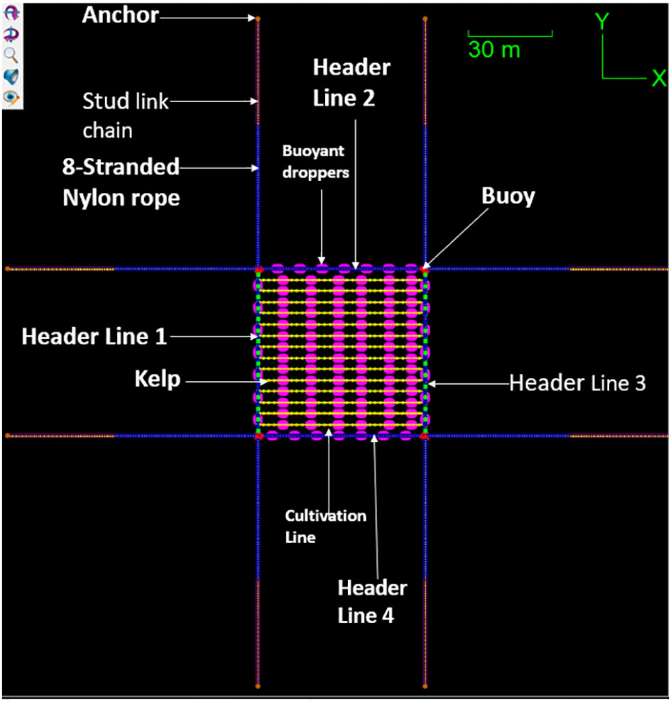
Figure 1 Plan view of offshore seaweed farm.

Figure 2

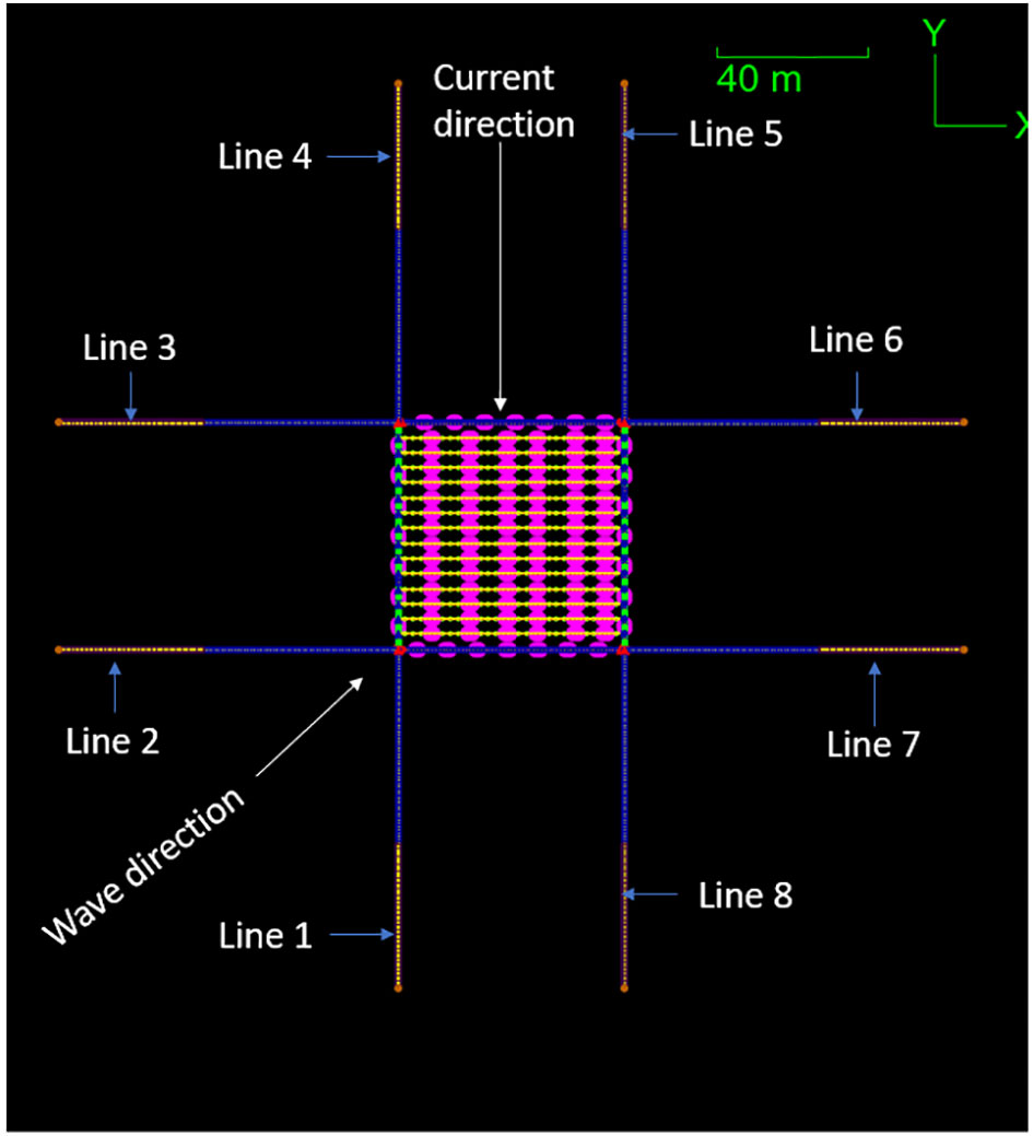
Figure 2 Model 1.

To design reasonable kelp farms, the two different types of offshore seaweed farm models with varying mooring arrangements are presented and tested, as depicted in Figures 2 and 3. The objective is to identify the design that exhibits lower tension on the mooring lines and possesses high structural integrity.

Figure 3

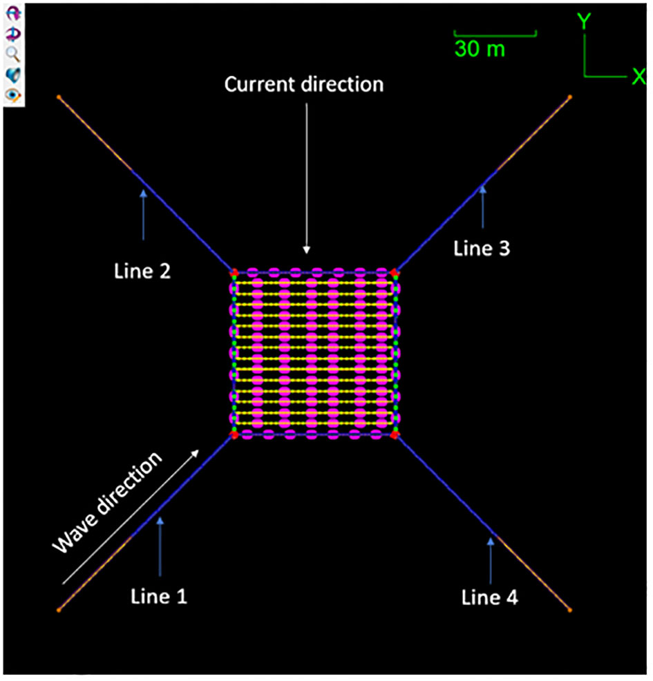
Figure 3 Model 2.

Following a thorough evaluation, the design of Model 1 is selected, as illustrated in Figure 2. This kelp farm comprises of 8 mooring lines that are securely anchored at a seabed depth of 50m. These mooring lines are connected to four buoys. The header line of Model 1 is constructed using a 60m-long 8-stranded nylon rope with a diameter of 0.06m. The total length of the mooring line is 100m, with the first 60m consisting of nylon rope and the remaining 40m composed of stud link chain, anchored at the seabed. The header lines and cultivation line of Model 1 and 2 are attached with smaller buoyant droppers. The buoyant droppers are attached at 8m intervals on the header lines and 10m intervals on the cultivation line for Model 1 and 2. The seaweed is kept 2.3m below sea surface. Model 2, illustrated in Figure 3, comprises of four mooring lines that are securely anchored at a seabed depth of 50m. These mooring lines are connected to four buoys, spread out at an angle of 45 degrees. The header line of Model 2 is constructed using a 60m-long 8-stranded nylon rope with a diameter of 0.06m. The total length of the mooring line is 100m, with the first 60m consisting of nylon rope and the remaining 40m composed of stud link chain, anchored at the seabed. These offshore seaweed farm models and their distinct mooring arrangements serve as a basis for comprehensive analysis and comparison. By examining the performance and structural characteristics of each model, valuable insights can be gained regarding their suitability and effectiveness in supporting offshore seaweed farming operations. These offshore seaweed farm models and their distinct mooring arrangements serve as the basis for comprehensive analysis and comparison. The mass of each buoy used in Model 1 and 2 was carefully implemented to ensure sufficient buoyancy and stability for the overall system of the offshore seaweed farm under different design scenarios.

Figures 1, 2 show the numerical model of a modular offshore seaweed farm structure. Table 1 provides an overview of the essential components of the farm design, outlining the significant parameters such as material choices and sizes that define these components. The seaweed cultivation lines are designed at 2.3m below sea surface. Table 2 provides the detailed structural parameters of kelp farm components. Table 3 provides the hydrodynamic parameters. Drag diameter equals normal drag reference area per length, or tangential drag reference area per length.

Table 1

Table 1 Major parameters defining offshore seaweed farm structure.

Table 2

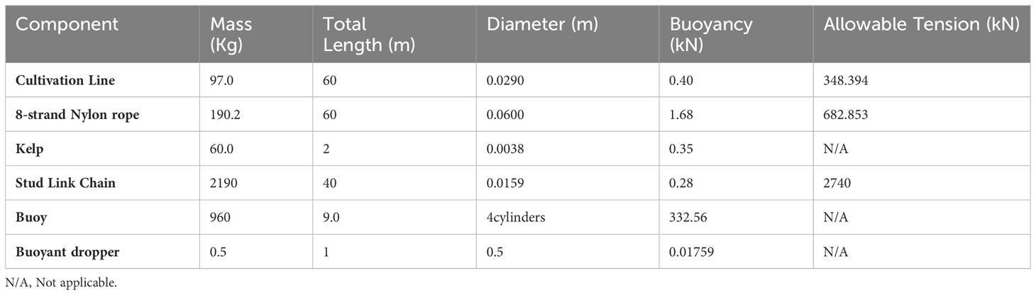
Table 2 Structural parameters of farm components.

Table 3

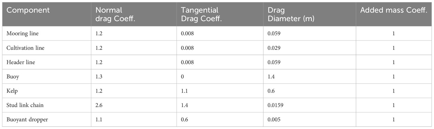
Table 3 Hydrodynamic parameters of the farm components.

3 Method of kelp farm model

Fiber ropes are simulated as line type with flexible linear elements. Lines are represented by using a lumped mass method (Heffernan, 2017). That is, the line is modeled as a series of ‘lumps’ of mass joined together by massless springs. Ropes are represented using linear elastic elements, which are assigned specific values for diameter, density, modulus of elasticity, and length. The stud link chain is modeled by a general line type, where the axial, bending and torsional stiffness are set directly. Similarly, mass is given per unit length, rather than calculated from a material density. This direct approach gives complete control over the data, allowing the analysis of flexible risers, umbilical, hoses, mooring chains, ropes, wires, bundles, seismic arrays, power cables, nets etc. The strands of seaweeds are represented as linear elastic elements attached to the line. The attachment type is defined by its weight, diameter, and arc length at which it is attached to the line. OrcaFlex models the buoyant dropper as a clump line attachment. The clump attachment can be buoyant or heavy and represents a small body that experiences forces (weight, buoyancy, drag etc.). But instead of being free to move, it is constrained to move with the node to which it is attached. The clump adds to the mass, buoyancy and hydrodynamic force to the line through its node. The properties of the line attachment themselves are given separately on the attachment types data form, allowing the same set of attachment properties to be used for a number of different attachments. The seaweed was attached at 2m intervals on the cultivation line. The structural mechanics of offshore seaweed farms are investigated in the following sections. OrcaFlex (https://www.orcina.com/orcaflex/), a commercial FEM and multibody physics software package, specializes in evaluating the loading and movement of rigid floating bodies moored by flexible anchor lines. OrcaFlex relies on finite element analysis and multibody dynamics to simulate the hydrodynamic forces and response of marine structures subjected to waves, currents, and wind. Marine structures are modeled as flexible and rigid elements in the form of lines, 6- or 3-degree-of-freedom buoys, and rigid body elements (Moscicki et al. 2022).

3.1 Static analysis

The hydrodynamic analysis of offshore seaweed farms also forms a fundamental component of this research. Understanding the flow characteristics around seaweed structures is essential for predicting the drag forces acting on the plants and determining their motion and stability. OrcaFlex uses steady hydrodynamic forces and catenary equations, an iterative approach using the multi-dimensional form of Newton’s method to find positions and orientations for each element in the model such that all forces and moments are in equilibrium.

Given a system of n equations with unknowns: F(x) = 0, where F: Rⁿ ≥ Rⁿ is a vector-valued function, and x = (x₁, x₂, …, x_n) represents the vector of unknowns. The multidimensional form of Newton’s method iteratively updates an initial guess x₀ for the solution by using the Jacobian matrix of F, denoted as J (F), and the current estimate x_k as shown in Equation (1):

$\begin{array}{ll}{x}_{\text{k}+1} = x_{\text{k}} - J(F){(x_{\text{k}})}^{-1}\times F(x_{\text{k}})& (1)\end{array}$

where J(F) (x_k) is the Jacobian matrix evaluated at x_k, and J(F) (x_k)^-1 denotes the inverse of the matrix. The Jacobian matrix J(F) is an n×n matrix, where each entry J_ij(F) represents the partial derivative of the i–th equation with respect to the j–th unknown. It can be written as shown in Equation (2):

$\begin{array}{ll}\text{J}\left(\text{F}\right)=\left[\begin{array}{c}\begin{array}{ccc}\frac{\partial {\text{F}}_1}{\partial {\text{x}}_1}& \frac{\partial {\text{F}}_1}{\partial {\text{x}}^2}\dots & \frac{\partial {\text{F}}_1}{\partial x_n}\\ \frac{\partial {\text{F}}_2}{\partial {\text{x}}_1}& \frac{\partial {\text{F}}_2}{\partial {\text{x}}^2}\dots & \frac{\partial {\text{F}}_2}{\partial x_n}\\ ⋮& ⋮& ⋮\end{array}\\ \begin{array}{ccc}\frac{\partial F_n}{\partial {\text{x}}_1}& \frac{\partial F_n}{\partial {\text{x}}_2}& \frac{\partial F_n}{\partial x_n}\end{array}\end{array}\right]& (2)\end{array}$

Where $\partial F_{\text{i}}/\partial x_{\text{j}}$ represents the partial derivative of the i–th equation with respect to the j–th unknown. The iteration continues until a desired level of accuracy is achieved or until a maximum number of iterations is reached. This is done to provide a starting configuration or static analysis solution for a dynamic simulation.

3.2 Dynamic analysis

The dynamic simulation uses the static analysis as its initial configuration and time then evolves forward from there. OrcaFlex uses numerical time-stepping algorithms to solve the fully nonlinear Equation (3) in the time domain.

$\begin{array}{ll}M(p,a)+C(p,v)+K(p)=F(p,v,t)& (3)\end{array}$

where, M(p, a) is the system of inertia load, which is related to the mass matrix, added mass matrix and position vector of the system; C(p, v) is the system damping load, which is related to damping matrix and velocity vector of the system; K(p) is the system stiffness load, whichi is related to stiffness matrix and vector, F(p, v, t) is the external load, which reflects the wind, wave and current environmental loads of the systems; here, p, v and a are the position, velocity, acceleration vectors repectively, and t is the simulation time. Equation (3) is the simply description about Cummmin’s equation.The more information about the application of Cummin’s theory and applicaiton can be found (Qiao et al., 2020; Li, 2021a; Li, 2021b; Huang et al., 2023; Li et al., 2023, Li and Wang, 2023; Wang et al., 2023). Especitally, Li and Wang (2023) give the detailed about theory and modeling of offshore floating complex operations, these will be helpful to understand the theory of dynamic analysis of mooring systems for floating structures.

Equation (3) is solved using implicit integration schemes. This time domain solution re-compute the system geometry at every time step and so the simulation takes full account of all geometric nonlinearities, including the spatial variation of both wave loads and contact loads. The forces and moments acting on each free body and node are then calculated. Forces and moments considered include weight, buoyancy, hydrodynamic and aerodynamic drag, tension and shear, bending and torque, seabed reaction and friction, contact forces with other objects, and forces applied by links and winches. The equation of motion (Newton’s law) is then formed for each free body and each line node as shown in Equation (4).

$\begin{array}{ll}M(p,a)=F(p,v,t)-C(p,v)-K(p)& (4)\end{array}$

Before the main simulation stage(s) there is usually a build-up stage, during which wave and vessel motions are smoothly ramped up from zero to their full size. This gives a gentle start to the simulation and helps reduce the transients that are generated by the change from the static position to full dynamic motion. OrcaFlex uses the extended form of Morison equation formulation to incorporate the relative movement between structural components and the surrounding fluid to estimate the hydrodynamic loading on the structures during each time interval. To account for the penetration of the water surface, the simulation adjusts the buoyancy, drag, and added mass of the affected components based on their submerged volume. This can be described by Equation (5).

$\begin{array}{ll}dF=\frac{1}{2}\rho D{C}_d\left|U_f-U_s\right|(U_f-U_s)+\rho A(1+C_a)\dot{U_f}-\rho A{C}_a\dot{U_s}& (5)\end{array}$

where D is the characteristic drag diameter, Cd is the drag coefficient, A is the cross-sectional area, Ca is the added mass coefficient, U_f is the transvers directional fluid particle velocity, and U_s is the transverse directional structure velocity. OrcaFlex simulations enable the dynamic adjustment of added mass and drag coefficients according to changing parameters like the Reynolds number in each time step. The simulation specifies the current and wave conditions at the beginning and does not modify them based on their interaction with the structure.

3.3 Fluid model hydrodynamics theory

The hydrodynamic loads on lines, 6D buoys are calculated by using an expanded version of Morison’s equation. Morison et al. (1950) initially proposed the equation to calculate wave loads on fixed vertical cylinders, incorporating two force components: one linked to water particle acceleration, representing the fluid inertia force, and another associated with water particle velocity, representing the drag force (Heffernan, 2017).

The original Morison's equation can be written as Equation (6):

$\begin{array}{ll}f=C_m\Delta a_f+\frac{1}{2}\rho C_{d}A\mid v_f\mid v_f& (6)\end{array}$

Where, f is the fluid force per unit length on the body. C_m is the inertia coefficient for the body. Δ is the mass of fluid displaced by the body. a_f is the fluid acceleration. ρ is the density of water. v_f is the fluid velocity. ρ is the density of water. C_d is the drag coefficient for the body. A is the drag area. v_f is the fluid velocity.

This principle is extended to a moving body, where the inertia term is reduced by $C_a\Delta a_b,$ and the drag term utilizes the body-relative velocity, resulting in the extended Morison’s equation, as shown in Equation (7):

$\begin{array}{ll}f=(C_m\Delta a_f-C_a\Delta a_b)+\frac{1}{2}\rho C_{d}A\mid v_r\mid v_r& (7)\end{array}$

Here: is the added mass coefficient for the body. a_b​ is the body acceleration relative to earth. v_r​ is the fluid velocity relative to the body. Typically, C_m​ is assumed to be 1+C_a. Simplifying the extended Morison’s equation can be written as (Heffernan, 2017), as shown in Equation (8):

$\begin{array}{ll}f=(\Delta a_f+C_a\Delta a_r)+\frac{1}{2}\rho C_{d}A\mid v_r\mid v_r & (8)\end{array}$

Here, a_r = a_f–a_b represents the fluid acceleration relative to the body. The term $(\Delta a_f+C_a\Delta a_r)$ denotes the inertia force, while the other term represents the drag force. The inertia force is comprised of two parts: one proportional to fluid acceleration relative to earth a_f (the Froude-Krylov component) and another proportional to fluid acceleration relative to the body a_r (the added mass component).

4 Environmental loads

The selected area for the model test and deployment is at Storm Bay, Tasmania, Australia, Latitude: - 43°08’24.00”S Longitude: 147° 31’ 48.00” E, as shown in Figure 4.

Figure 4

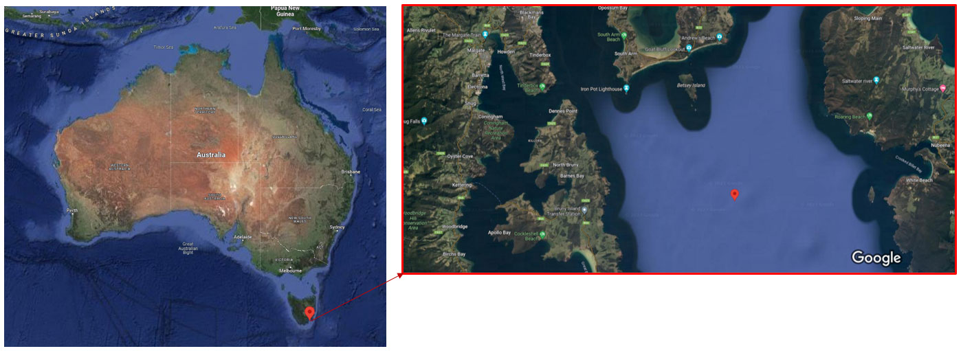
Figure 4 GPS coordinate for the selected site (s://latitude.to/articles-by-country/au/australia/117901/storm-bay).

A complete dynamic response analysis of the offshore seaweed farm design requires consideration of a wide range of wave conditions, including operational and extreme conditions. Therefore, in this study, the analyses are reported for environmental conditions with regular wave and irregular/random (JONSWAP) waves described by significant wave height (H_s), the zero-crossing period (T_z) and a constant sea current and wind speed. According to aquaculture industry standards, Norwegian standard of NS9415 (Norway Stardard 9415, 2021) typically suggests the application of waves or currents with a 50-year return period in design load cases for aquaculture structures. Extreme conditions for the study area were determined through statistical analysis of publicly available oceanographic data collected wave dataset ERA5 for the last 6 years (from 2013 to 2018) downloaded from the European Centre for Medium-Range Weather Forecasts (ECMWF) (Chu and Wang, 2020). ECMWF provides significant wave height H_s = 6.84 m and the zero-crossing period T_z=9.4s and current speed of 0.81 m/s. From the wave raw data, 50-year (EC3) return period sea states can be statistically estimated using the probability distribution function (PDF) of Gumbel distribution (Chu and Wang, 2020). Hence, in the present simulation, for the regular wave and irregular (JONSWAP) wave cases, both wave heights are 6.84 meter, the wave direction is set as 45 deg. For the JONSWAP wave case, the peak period is set as 9.4 second. For the regular wave case, the period is 9.4 second. In addition, the current speed is 0.81m/s and the current direction is 270 deg in these two simulation cases.

5 Numerical results and discussions

Two numerical models of offshore seaweed farm were developed. Each of the models was subjected to both regular and irregular waves as described in Section 4. The simulation time was set to 1200s at times steps of 0.01s with a maximum iteration of 500.

5.1 Numerical results

5.1.1 Buoy heave motion and elevation

The maximum buoy elevation values for the two models subjected to environmental loads are shown in Figures 5–8. Model 1 and Model 2 are subjected to random wave loading and regular monochromatic wave. The heave movement of the buoy for both models is compared.

Figure 5

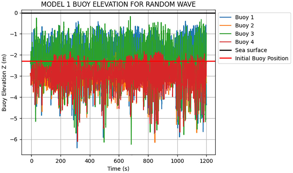
Figure 5 The heave motion of buoys in Model 1 for random wave.

Figure 6

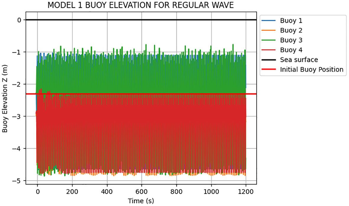
Figure 6 The heave motion of buoys in Model 1 for regular wave.

Figure 7

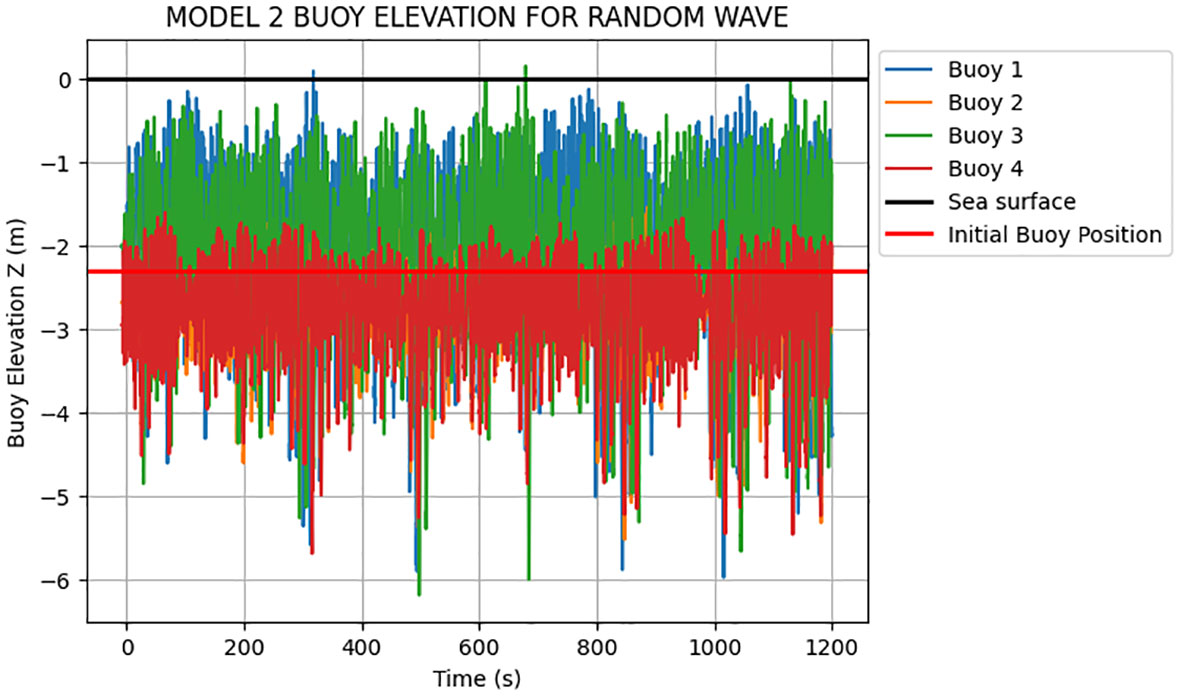
Figure 7 The heave motion of buoys in Model 2 for random wave.

Figure 8

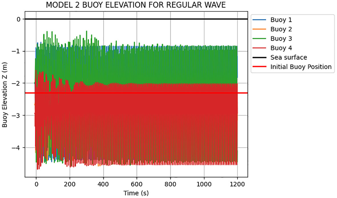
Figure 8 The heave motion of buoys in Model 2 for regular wave.

Two different wave types are used in case 1 for regular waves and case 2 for irregular waves, as shown in Section 4. The initial stack base (z) position of buoy which serves as initial reference point of the buoy posiition is -2.3m submerged. Comparing the buoy elevation of Model 1 subjected to random wave with the buoy elevation of Model 1 subjected to regular wave, as shown in Figures 5 and 6, it can be observed that the buoy heave movement and elevation for the random wave of Case 2 is higher than that in the regular wave of Case 1.

In addition, comparing the maximum buoy elevation of Model 2 subjected to random wave with the buoy elevation of Model 2 subjected to regular wave, as shown in Figures 7 and 8, it can be observed that, the heave movement of model subjected to random wave is higher than the one of Model 2 subjected to regular wave. Comparing Model 1 and Model 2, it can be observed that the buoy heave movement is higher in Model 2 almost piercing the surface of the sea as compared to the lower heave movement in Model 1. Note that the irregular nature of the buoy heave movement of the models when subjected to random wave and the steady pattern of buoy heave motion when the models are subjected to regular. In summary, the irregular and unpredictable nature of random waves makes it more challenging for the buoyancy system of an offshore seaweed farm to adapt to the changing wave conditions. Consequently, the buoy heave movement tends to be higher in random wave spectra compared to regular wave. Since the mooring line attached to the buoy has paid out length which allowed the line to extend and retract during up and down movement. The sinusoidal motion of the buoy is determined to be caused by the time-varying wave elevation. This motion occurs because the mooring line connected to the buoy has a specific length that allows it to extend and retract as the waves move up and down.

5.1.2 Effective tension of mooring lines

Figure 9 shows the maximum tension in the entire length of the mooring line when Model 1 is subjected to random wave, respectively, while Figures 10 shows the maximum tension in the entire length of the mooring line when Model 2 is subjected to random waves, respectively. The mooring line is anchored at the seabed and represented at the position of 100m length of the mooring line, whilst the fairlead is attached to the buoy and represented at the position of 0m on the mooring line as shown in Figures 9 and 10. The tensile forces for the two models are analyzed and compared to check whether they are over the breaking load limit or not. From the parameters shown in Table 2, the breaking load for the mooring lines is given as 682.853 kN. It is observed that none of these mooring lines has exceeded their breaking load limit. However, it can be observed in Figures 9 through 10 that, in environmental conditions (random waves) Model 2 has the higher mooring tension while Model 1 has the lower mooring tension at both anchor and fairlead. Lower mooring tension in Model 1 implies reduced cyclic loading on the mooring system, which can result in decreased fatigue damage. Fatigue damage accumulation can lead to failures in the mooring components over time. Therefore, the lower tension levels of Model 1 indicate potentially longer service life and reduced maintenance requirements. A more stable mooring system in Model 1 allows for better control and positioning of the seaweed farms. This stability helps to maintain the desired orientation and minimizes the risk of dislodgement or drifting. As a result, Model 1 can potentially achieve higher productivity and operational efficiency compared to Model 2. It can also be observed that the mooring tension in all models when subjected to random waves are higher than the tension when subjected to regular waves. This can be attributed to the nonlinear effects in the response of the mooring system and the wide range of wave heights, periods, and directions, which leads to greater variability compared to regular waves.

Figure 9

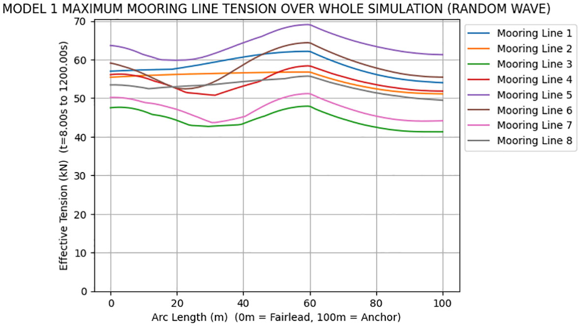
Figure 9 Mooring line tension of Model 1 for random wave.

Figure 10

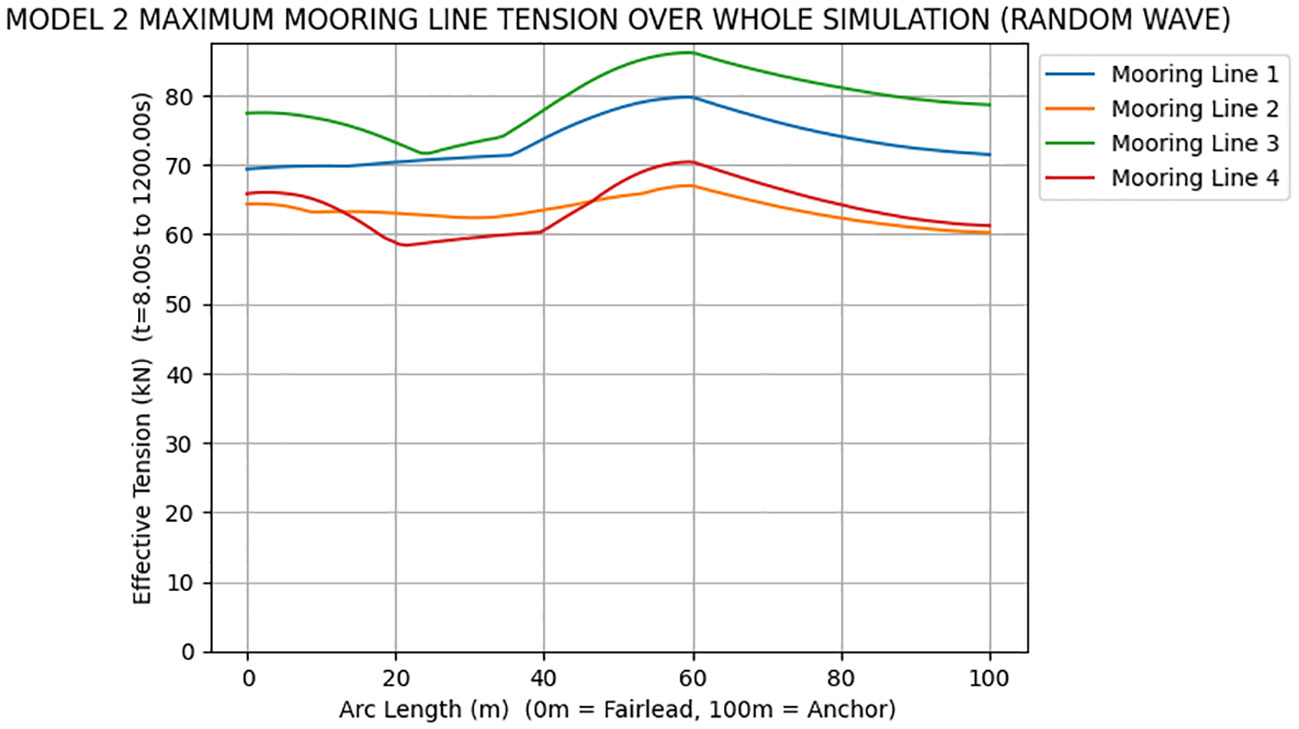
Figure 10 Mooring line tension of Model 2 for random wave.

From Table 4, it can be observed that maximum tension at fairlead of mooring lines in Model 2, when subjected to random waves experience higher tensions as compared to mooring line tension when subjected to regular waves. As shown in Section 4, the environmental loading conditions including wave height, period, direction, current speed, and current direction for both random wave and regular waves were the same and comparable. The mooring peak tensions and system response at fairlead and anchor for both random and regular wave were compared. According to Table 4, it can be noticed that the line tension at fairlead for random wave experiences an increasing percentage of 18.40% in mooring Line 3 and lowest in Line 2 at 7.4%. This can be attributed to the differences in wave characteristics, wave energy distribution, resonance and interference, between random waves and regular waves. Random waves exhibit a wide spectrum of wave heights, periods, and directions. They are more realistic representations of natural wave conditions. The broad spectrum of random waves can lead to resonance and interference effects, causing varying tensions in the mooring lines as different wave components interact with the system. Whereas regular waves have constant wave characteristics, including wave height, period, and direction. They are simplified representations for analytical purposes. Regular waves are less likely to cause resonance or interference effects due to their single-frequency nature. The nonlinear effects in the response of the mooring system and wide range of wave heights, periods, and directions, led to greater variability of mooring tension in random waves compared to regular waves.

Table 4

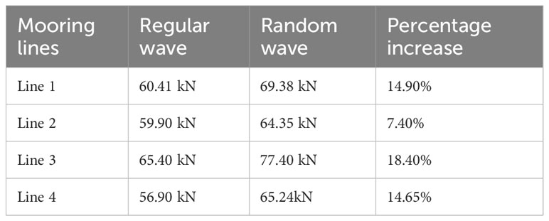
Table 4 Comparing maximum tension at fairlead of mooring lines in Model 2 under environmental load cases.

5.1.3 Tension of planting lines for two models

Figure 11 shows the tensile forces exerted on planting lines for the two preliminary models under certain period of time for random waves, respectively. It is observed that the tension forces on planting lines in the two models subjected to random wave did not exceed the planting line breaking load limit which is 348.394 kN. The tensile forces in planting lines as shown in Figure 11 subjected to randon waves reveals that, most of cultivation line tension for Model 1 is lower than the tension force of cultivation lines in Model 2. Similar phenomenon that the tensile forces in cultivation lines for Model 1 are lower than that of Model 2, when the systems are subjected to regular wave loads. In summary, Model 1 has the least tension in planting lines, while Model 2 has the highest tension. Thus, the planting lines in Model 1 are much more suitable for seaweed farming than those in the Model 2.

Figure 11

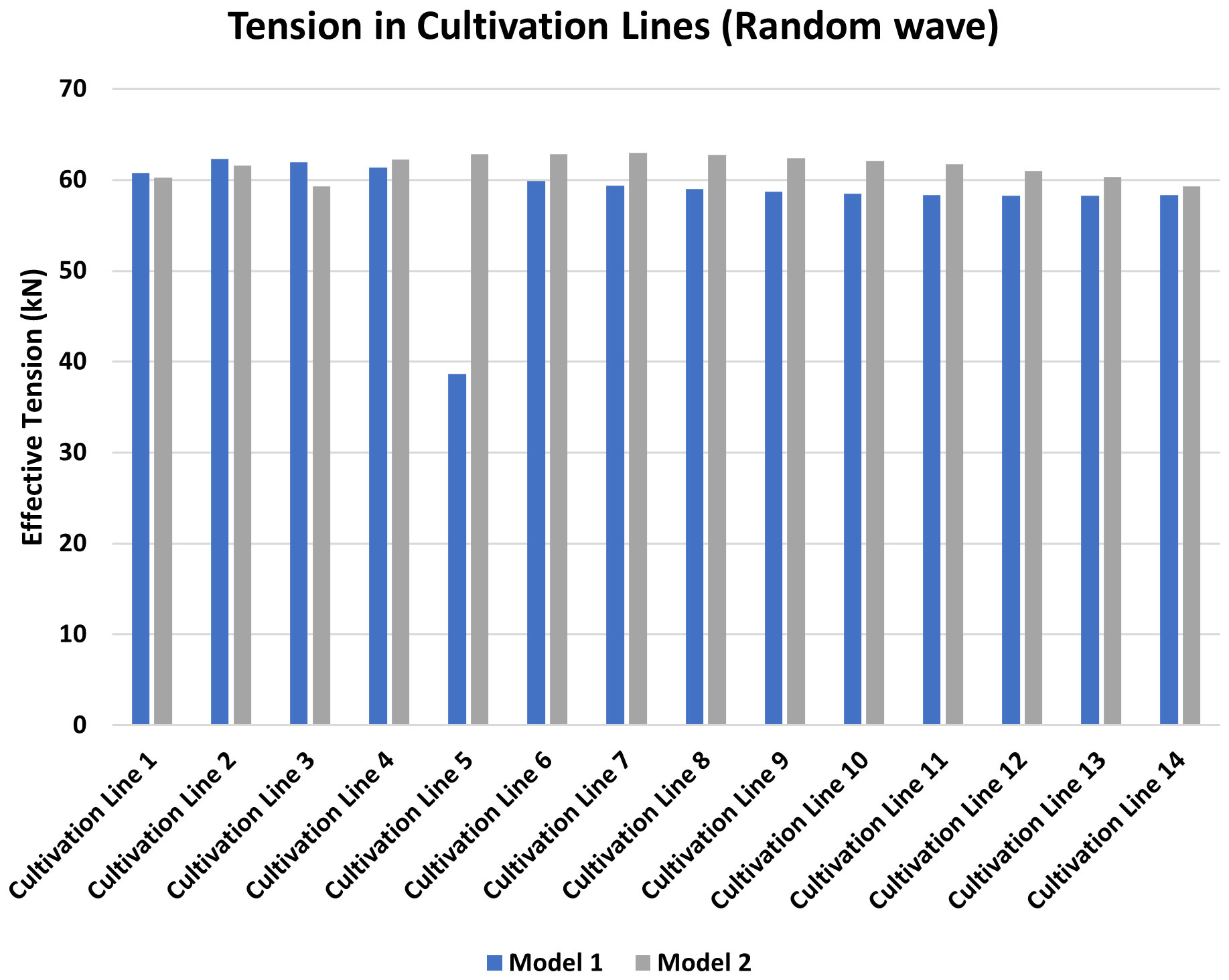
Figure 11 Tension of planting lines for random wave.

5.1.4 Maximum tension in header lines

Figures 12, 13 show the maximum tension in headlines along the entire length. According to Figures 1, 12, 13, it can be observed that tension in header line 1 and header line 3 at rigid ends for both models are higher than tension in header line 2 and header line 4. This can be attributed to load distribution. The cultivation lines carrying the seaweed impose additional loads on the connected header lines. Since Header Line 1 and Header Line 3 are connected to the cultivation lines, they are directly subjected to the additional load induced by the weight and drag forces of the seaweed. This additional load leads to higher tension in Header Lines 1 and 3 compared to Header Lines 2 and 4, which do not carry any extra load. However, none of this header lines for either model 1 or 2 exceeds its breaking load limit, which could potentially cause the collapse of the offshore seaweed farm. In addition, the tension values of Header Lines 1 and 3 in Model 1 is lower than the values of Header Lines 1 and 3 in Model 2 by comparing Figure 12 with Figure 13. In addition, the tension response of the header lines for Model 1 and Model 2 under the regular wave are lower compared to that under the random waves. Based on the above results of Section 5.1, Model 1 is a more suitable design for keeping the structural integrity of kelp farms because the tension values of mooring lines and cultivation lines in Model 1 are lower than those in Model 2.

Figure 12

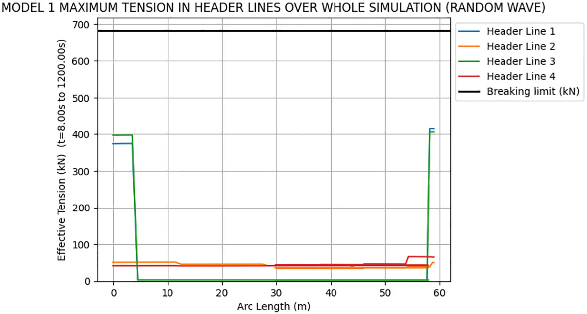
Figure 12 Model 1 tension in header lines for random wave.

Figure 13

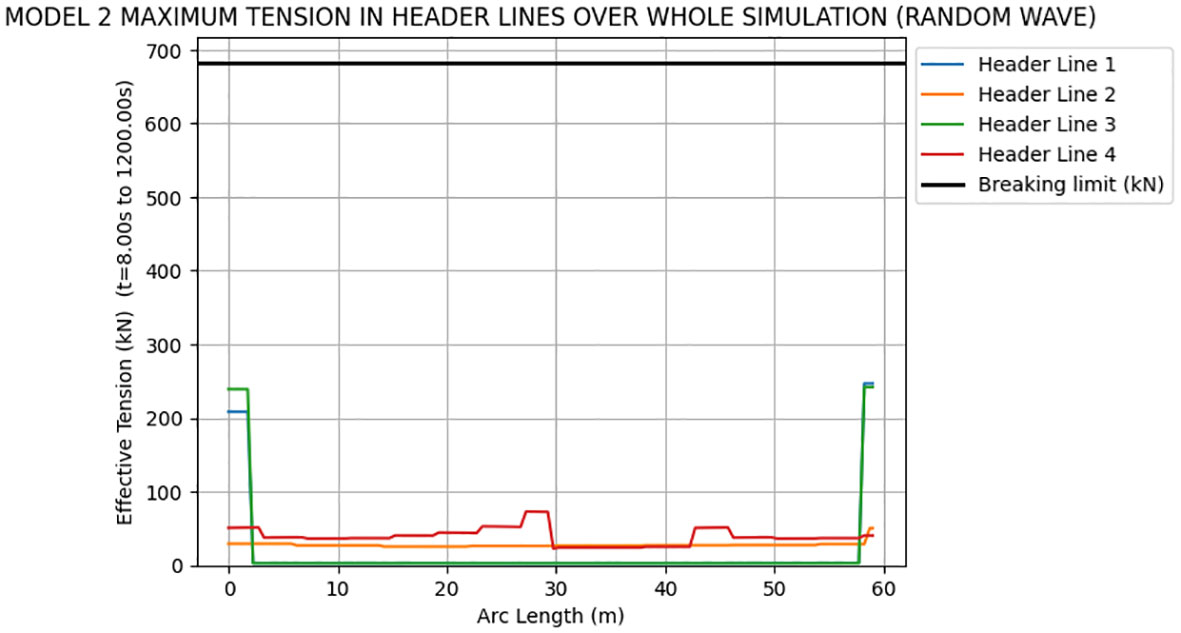
Figure 13 Model 2 tension in header lines for random wave.

5.2 Model validation

Model validation is a crucial aspect of any simulation study, ensuring the accuracy and reliability of the computational model. This approach provides a means to assess the fidelity of the simulation by examining how well it reproduces the outcomes reported in a reputable source. Through this comparative analysis, it is possible to establish the credibility and robustness of capturing the dynamic behavior of the offshore seaweed farm in the present study. For validation, the published paper titled Numerical Modelling of a Mussel Line System by Means of Lumped-Mass Approach published by Pribadi et al. (2019) will be simulated using OrcaFlex. The simulated results of the dynamic response of the Mussel Line System will be compared to the published results.

5.2.1 Description of mussel longline system

The longline system configurations (depicted in Figure 14) employ a semi-submerged system comprising an extended central line connecting two spar-type buoys, which serves as the backbone supporting mussel collector lines. The dry mass, the outer diameter, length, and volume, are set as 2500kg, 0.790meter, 8.865meter, 4.345m³. Key characteristics of the mooring arrangement for these experimental setups are presented in Tables 5 (Pribadi et al., 2019).

Figure 14

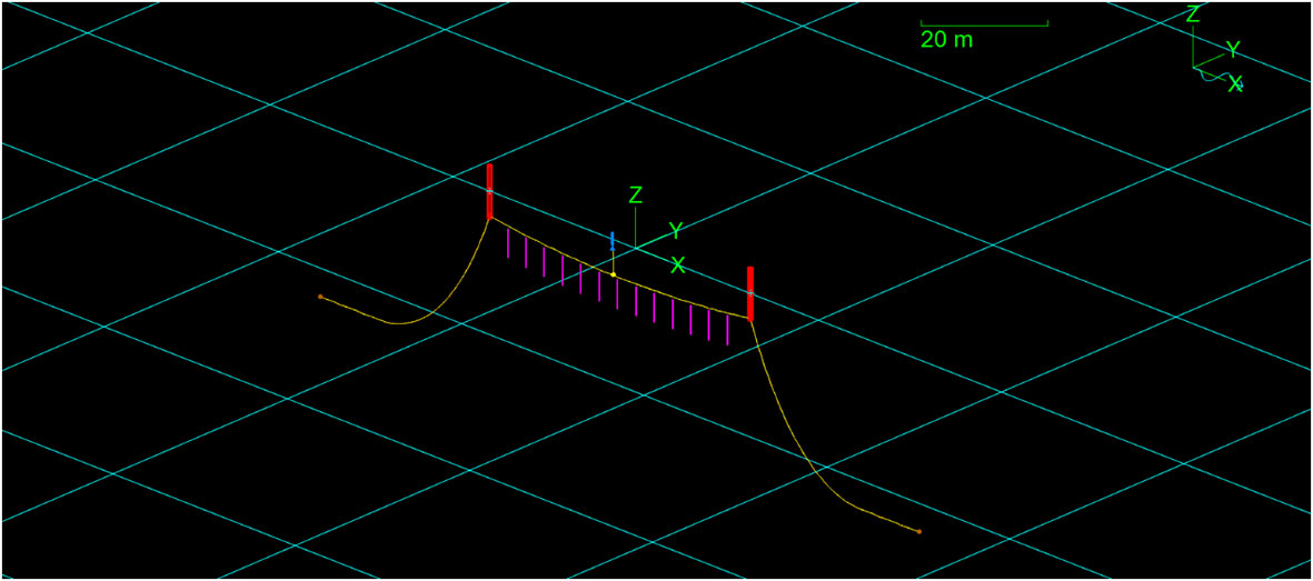
Figure 14 Numerical model of the longline cultivating system.

Table 5

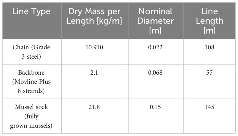
Table 5 Line componnet properties of the longline system.

This system, featuring partially submerged crop lines, is anticipated to undergo reduced mooring line loads due to its deeper submersion. The chain is discretized into 12 contiguous segments, each resembling a homogeneous cylinder. Drag coefficients are suggested based on the chain’s equivalent diameter utilized in the numerical computations. The seabed is represented as a flat bottom or constant bathymetry with a depth of 30 meters, the buoy is set at the depth of 4.43 meter. The mooring radius, which is the horizon distance between the nearby buoy and anchor, set as 30 meters (Pribadi et al., 2019).

5.2.2 Environmental load of mussel longline system

In terms of the environmental loads, the setup experiences a regular wave with an amplitude of 5 meters and a period of 8.33 seconds (corresponding to a wavelength of 103 meters), as detailed in the work by Pribadi et al. (2019). The wave propagates along the positive x-axis.

5.2.3 Model validation results and discussion

The time series of the buoy’s heave motion position calculated in MoorDyn by the publisher (Pribadi et al., 2019) and the time series of buoys position in OrcaFlex model are compared and analyzed. The comparison between minimum and maximum values of buoy’s heave (z) motion results are listed in Table 6. Good agreement can be found for heave motion between the published results of Mordyn, according to the reference (Pribadi et al., 2019) and the simulated model results in Orcaflex. The substantial agreement witnessed between the simulated buoy’s z positions over the entire 150-second simulation duration signifies a robust validation outcome, providing confidence in the accuracy of the model. This positive alignment suggests that the simulation faithfully replicates the expected behavior of the buoy under the specified conditions. Several contributing factors bolster the success of this validation.

Table 6

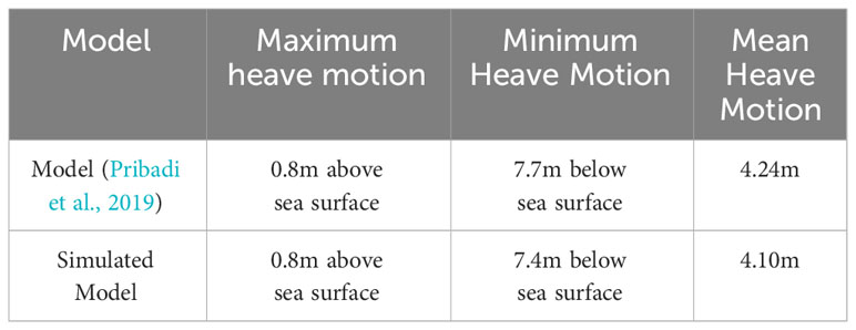
Table 6 Comparison between the buoy heave motion of (Pribadi et al., 2019) and the present simulated model.

The model accurately captures and represents the environmental conditions, such as regular waves or other external forces that influence the buoy’s dynamics during the simulation. The simulation incorporates a precise definition of the buoy system’s dynamics, including the mooring configuration and the buoy’s response to loading conditions. This ensures that the model employs realistic and reliable values, contributing to the accuracy of the simulation.

All conditions during the validation, including initial conditions and applied forces, were maintained consistently. Consistency in simulation conditions enhances the reliability of the validation process. In summary, the observed agreement in the buoy’s positions underscores the effectiveness of the model validation, affirming we have the capability to replicate the behavior of the buoy under the specified conditions. This positive outcome enhances the overall confidence in the accuracy and reliability of the present simulation model.

6 Economic analysis

The decision-making process for selecting the most suitable offshore seaweed farm model involves not only considering the mooring analysis and structural integrity but also conducting a comprehensive analysis of capital expenses. The analysis of capital expenses plays a crucial role in evaluating the financial feasibility and cost-effectiveness of offshore seaweed farm models. This analysis focuses on the initial investment required to construct the farm facilities, including mooring systems, buoys, header lines, cultivation lines, labor expenses, and installation costs to provide a comprehensive overview of the capital expenses associated with each model. A basic capital expenses to gross income and initial rate of return assessment was conducted. The assessment was limited to capital expenses required for purchasing farm components for Model 1, Model 2 and longline cultivation system on the same sea surface area (60m×60m), as shown in Figure 15. Farm equipment, seed costs, and farm-gate crop values were estimated from current market values. By examining the capital expenses for Model 1, Model 2 and longline cultivation system, we can gain valuable insights into the cost implications of each design to determine the most cost-effective option or more economically viable option for commercial-scale offshore seaweed cultivation. An integrated approach, considering both technical and economic aspects, enables stakeholders to make informed decisions and support the sustainable development of offshore seaweed farming.

Figure 15

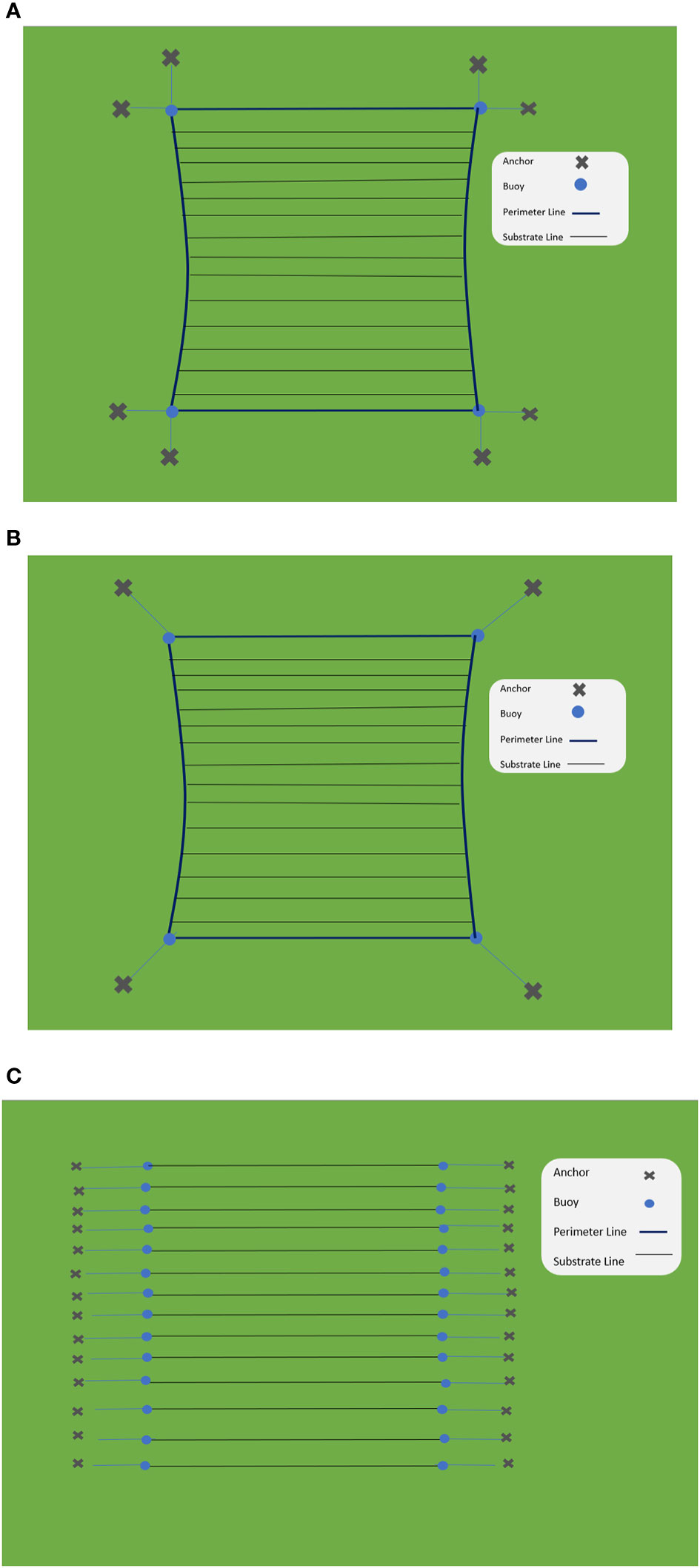
Figure 15 Kelp farms with three models with the same size. (A) Model 1 of the farm size(60m×60m). (B) Model 2 of the farm size(60m×60m). (C) Longline systems of the farm size(60m×60m).

6.1 Capital expenses and operational cost

A single grid of Model 1 comprises of eight mooring lines and four main buoys, providing a robust anchoring system for the offshore seaweed farm. The mooring line is constructed using a 100m-long 8-stranded nylon rope with a diameter of 0.06m for the first 60m, and a stud link chain for the remaining 40m, anchored at the seabed. The cultivation line is constructed using a 60m-long 8-stranded nylon rope with diameter 0.03m. The construction costs of Model 1 mainly consist of materials, labor, and installation expenses for a size of 60m×60m. This farm size will incorporate 8 mooring lines, 8 anchors, 4 buoys, 4 header lines and other components, as shown in Figure 15A. Additionally, costs associated with underwater construction and installation might be higher due to the complexity of the mooring arrangement. Due to 8 mooring lines and anchors in Model 1, Model 1 is expected to have a higher initial construction cost compared to Model 2 with 4 moorings. However, a detailed cost estimation is necessary to determine the exact difference. Model 2 comprises of 4 mooring lines, arranged at an angle of 45 degrees. Similar Model 1, it also requires a 100m-long nylon rope with a diameter of 0.06m for the first 60m, and a stud link chain for the remaining 40m, anchored at the water area with 50 meters. Model 2 with the size of 60m×60m includes 4 mooring lines, anchors and buoys, as shown in Figure 15B. The cultivation lines are constructed using a 60m-long nylon rope with a diameter of 0.03m. The construction costs of Model 2 will be lower than Model 1 due to the reduced number of mooring lines. Additionally, the simpler mooring arrangement might result in easier installation procedures, further contributing to cost savings.

A single traditional long-line cultivation system comprises two mooring lines and two buoys, according to Pribadi et al. (2019). The mooring lines in the longline system require a 100m-long nylon rope with a diameter of 0.06m for the first 60m and a stud link chain for the remaining 40m, anchored at the water area with 50 meters. The longline has only one cultivation line and is constructed using a 60m-long nylon rope with diameter of 0.06m. The construction costs of the longline cultivation on a farm with the size of 60m×60m will incorporate 14 cultivation lines, 28 buoys and 28 anchors, as shown in Figure 15C. The longline system will be more expensive in construction cost than models 1 and 2 due to the increase of mooring lines, buoys, and anchors.

6.1.1 Material costs

The material costs include the expenses for ropes, chains, buoys, cultivation lines, and other necessary components. Model 1, Model 2 and the traditional longline utilize 8-stranded nylon ropes and stud-link chains for their mooring lines, and all use nylon ropes for their header lines and cultivation lines. The costs of these materials depend on market prices and the required quantities. In the description of the models, it was mentioned that the mass of each buoy used in Model 1 and Model 2 was carefully implemented to ensure sufficient buoyancy and stability. The cost of designing and manufacturing buoys with specific mass and stability characteristics will contribute to the overall capital expenses. According to Figure 15, the main difference of these three models is the number of mooring lines. Hence, the material cost of mooring components of kelp farms is listed in Table 7.

Table 7

Table 7 List of main components of Kelp Farms (Source from St-Gelais et al., 2022).

6.1.2 Labor expenses

The labor expenses encompass the costs associated with the installation of mooring lines, buoys, header lines, and cultivation lines. Model 1, with its more extensive mooring system, might require additional labor hours for installation, compared to Model 2 and the longline cultivation system. The labor costs depend on local labor rates and the expertise required for underwater construction. The man hours for the installation are estimated, as listed in Table 8 (St-Gelais et al., 2022).

Table 8

Table 8 Man-hours required to construct offshore seaweed farm (St-Gelais et al., 2022).

Following the Fair Work Commission (FWC) Annual Wage Review 2022-2023, the Australian national minimum wage has now increased to $23.23 per hour (The 2023 Australian Minimum Wage Increase, 2023). We estimate an hourly labor rate in the Australian marine industry to be about $45. In that regard, the labor cost per person of construction and deployment of Model 1 costs $7200, Model 2 costs $3600, whereas the 14 longline cultivation systems costs $25200.

6.1.3 Equipment costs

Specialized equipment, such as winches, cranes, and underwater construction tools, may be necessary for the installation of the offshore seaweed farm. The cost of renting or purchasing this equipment adds to the initial capital expenses. It is assumed that the cost of renting this equipment for these three models can be regarded as the same, because these types of equipment perform the same functions.

6.1.4 Installation costs

The installation costs are influenced by the complexity of the mooring system and the underwater construction project. Due to the complex mooring systems of Model 1,the installation costs of Model 1 is higher than those of Model 2. The transporting materials and equipment to the offshore location may also impact installation expenses which can also be estimated as similarly comparable. As required, a more spacious van is required to transport equipment to the loading boat/vessel for Model 1 as compared to Model 2. The traditional longline cultivation system will incur the highest installation cost, because the construction costs of the longline cultivation will incorporate 14 cultivation lines, 28 buoys and anchors.

6.2 Operational and maintenance costs

All three model systems have 14 cultivation lines with the length of 60m, supporting the growth of Laminaria japonica. These operational costs typically include seeding, harvesting, monitoring, and labor for cultivation management. Hence, the operation cost of these three cultivating systems may be almost the same.

In terms of the maintenance costs of the mooring systems, Model 1 might incur higher maintenance costs compared to Model 2, which has a simpler mooring arrangement. The longline cultivation system will incur the highest maintenance cost due to its increased number of buoys and mooring lines. The traditional longline cultivation system will incur the highest maintenance cost as compared to Models 1 and 2, while Model 2 incurs less maintenance cost than others.

6.3 Cost comparison and discussions

To assess the economic feasibility of establishing offshore seaweed farms, a cost comparison between Model 1, Model 2, and the longline cultivation system is essential.

It is crucial to consider both direct costs (e.g., material and labor) and indirect costs (e.g., equipment and transportation) for a comprehensive analysis. Assuming a 5-member team is considered for the operation and deployment of the offshore seaweed farm, the labor cost for Model 1 is $36000, while the labor cost for Model 2 is $18000, and the longline cultivation system will be $12600 according to Table 8. According to Table 7, the cost of constructing seaweed farm for Model 1 is approximately $27857.6, in addition to the labor cost of $36000, the total cost of Model 1 equals to $63857.6. The cost of constructing Model 2 is approximately $16494.4, in addition to the labor cost, the total cost of Model 2 equals to $34494.4. Note that, the cost of constructing the longline cultivation system will be $91873.6. If the labor cost is also included, the total cost of longline systems is $217873.6. Comparing the total cost of Models 1 and 2 with longline systems, we can find that the number of anchors and mooring lines leads to an increase in the total cost of building kelp farms. Hence, developing the optimal mooring systems will help to reduce the costs of building kelp farms.

Based on the situation of the same (14 lines) lines of all three kelp cultivating systems, we can assume that the potential revenue generated from seaweed products is the same. These three models are made up of 14 cultivating lines of 60 meters length. According to the research of (St-Gelais et al., 2022), the peak biomass of kelp in the cultivating lines was about 12.67kg/m (±0.4kg). Hence, the kelp yield of these kelp cultivation systems produced 10642.8kg (±336kg) wet weight total over 840(60m×14) meters length of cultivation lines. According to (https://www.selinawamucii.com/), the estimation wholesale price of seaweed is $10.5/wet kg in Australia. Considering the 7-month growth season of seaweed, we can estimate annual revenue of $111749.4 ($3528) for these three model cultivation systems with (60m×14) lines.

The (Return on Investment) ROI is a critical financial metric used to evaluate the profitability of an investment. It is calculated as the ratio of net profit to the total investment made over a specific period. A positive ROI indicates a profitable investment, while a negative ROI suggests a loss. If we assumed an 8% return on investment over 3 years for the type of longline cultivating system (St-Gelais et al., 2022), then the total investment of long cultivating systems is about $1396867.5. Hence, the common expense of the kelp seed, fuel, and infrastructure (vessel, truck, trailer, etc.) is about $1178993.9. If we assumed that the common expense of the seed, fuel, and infrastructure (vessel, truck, trailer, etc.) for Models 1 and 2 is equal to $1178993.9. The total investment of Model 1, which includes the investment of mooring part ($63857.6) and the common expense ($1178993.9), equals to $1242851.5. Similarly, the total investment of Model 2 is $1215168.3 ($1178993.9 + 36174.4). We can calculate that the ROI of Model 1 is 8.99% ($111749.4/$1242851.5), while the ROI of Model 2 is 9.20% ($111749.4/$1215168.3).

Note that ROI Factors, which include kelp yield, seaweed quality, expense of infrastructure, kelp farm size and pattern of mooring etc., can impact the ROI. Especially, we can see that the reducing costs of mooring systems for kelp farms can strongly affect the ROI of building kelp farms. While Model 1 appears to have better mooring analysis results and higher structural integrity, the economic analysis reveals that its capital expense is higher. Here, Model 2 presents a more economically viable option for seaweed farmers, while model 1 is the most expensive to build. However, to design the most economically viable and optimal of offshore kelp farms, further detailed lifecycle analysis of kelp farms should be performed in the future.

7 Conclusion

This paper presented a numerical analysis and simulation of an offshore seaweed aquaculture facility. This study also involved an economic analysis of the proposed offshore seaweed farm facility to enable stakeholders to make informed decisions and to support the sustainable development of the offshore seaweed farm facility. The study presented model simulations of offshore seaweed farm facilities, subjecting them to extreme environmental loads such as waves and currents. Among the seaweed platform models, Models 1 and 2 demonstrated the structural feasibility design, featuring a stable mooring arrangement with minimal tension exerted on each line within the model. The analysis encompassed estimating the tension on the mooring lines, planting lines, and header lines, comparing them to the line-breaking limit values. However, economic analysis were performed, the result showed that Model 2 is more economical than Model 1. The traditional longline cultivation system, which requires more lines than Modes 1 and 2, is the least economically viable option. The present numerical simulation would help to understand the dynamic response of offshore seaweed farms and help to design the optimal mooring system of kelp farms, which can strongly affect the economic feasibility of offshore seaweed farms.

Data availability statement

The original contributions presented in the study are included in the article/supplementary material. Further inquiries can be directed to the corresponding author.

Author contributions

YL: Conceptualization, Methodology, Project administration, Supervision, Validation, Writing – review & editing, Writing – original draft. SB: Writing – original draft. ZP: Investigation, Formal analysis, Validation, Writing – review & editing. JZ: Conceptualization, Funding acquisition, Writing – review & editing. WC: Funding acquisition, Supervision, Formal analysis, Writing – review & editing. GM: Project administration, Resources, Visualization, Writing – review & editing. SY: Supervision, Writing – review & editing.

Funding

The author(s) declare financial support was received for the research, authorship, and/or publication of this article. The research work is supported by National Key R&D Program of China (SQ2022YFB4200183), China Postdoctoral Science Foundation (Grant No. 2022M722820), the National Key R&D Program of China (2023YFC3007900), the National Natural Science Foundation of China (Grant Nos. 51979050), the Fund of State Key Laboratory of Coastal and Offshore Engineering (Grant No. LP2213), the Natural Science Foundation of Jiang-Su Province (Grant No. BK20201314), the Fund of State Key Laboratory of Hydraulic Engineering Simulation and Safety of Tianjin University (Grant No. HESS-1910),the Key R&D Program of Shandong Province, China (Grant Nos. 2023CXGC010407, 2020CXGC010702) and XPRIZE Carbon Removal Student Award (KelpFarmCareer Team).

Conflict of interest

The authors declare that the research was conducted in the absence of any commercial or financial relationships that could be construed as a potential conflict of interest.

Publisher’s note

All claims expressed in this article are solely those of the authors and do not necessarily represent those of their affiliated organizations, or those of the publisher, the editors and the reviewers. Any product that may be evaluated in this article, or claim that may be made by its manufacturer, is not guaranteed or endorsed by the publisher.

References

Abhinav K., Collu M., Benjamins S., Cai H., Hughes A., Jiang B., et al. (2020). Offshore multi-purpose platforms for a Blue Growth: A technological, environmental and socio-economic review. Sci. Total Environ. 734, 138256. doi: 10.1016/j.scitotenv.2020.138256

PubMed Abstract | CrossRef Full Text | Google Scholar

Ahmed Z. U., Hasan O., Rahman M. M., Akter M., Rahman M. S., Sarker S. (2022). Seaweeds for the sustainable blue economy development: A study from the south east coast of Bangladesh. Heliyon 8 (3), e09079. doi: 10.1016/j.heliyon.2022.e09079

PubMed Abstract | CrossRef Full Text | Google Scholar

Bak U. G., Gregersen Ó., Infante J. (2020). Technical challenges for offshore cultivation of kelp species: Lessons learned and future directions. Bot. Mar. 63 (4), 341–353. doi: 10.1515/bot-2019-0005

CrossRef Full Text | Google Scholar

Bak U. G., Mols-Mortensen A., Gregersen O. (2018). Production method and cost of commercial-scale offshore cultivation of kelp in the Faroe Islands using multiple partial harvesting. Algal Res. 33, 36–47. doi: 10.1016/j.algal.2018.05.001

CrossRef Full Text | Google Scholar

Buck B. H., Buchholz C. M. (2004). The offshore-ring: a new system design for the open ocean aquaculture of macroalgae. J. Appl. Phycol. 16, 355–368. doi: 10.1023/B:JAPH.0000047947.96231.ea

CrossRef Full Text | Google Scholar

Buschmann A. H., Camus C., Infante J., Neori A., Israel Á., Hernández-González M. C., et al. (2017). Seaweed production: overview of the global state of exploitation, farming and emerging research activity. Eur. J. Pshycology 52 (4), 391–406. doi: 10.1080/09670262.2017.1365175

CrossRef Full Text | Google Scholar

Campbell I., Macleod A., Sahlmann C., Neves L., Funderud J., Øverland M., et al. (2019). The environmental risks associated with the development of seaweed farming in europe - prioritizing key knowledge gaps. Front. Mar. Sci. 6. doi: 10.3389/fmars.2019.00107

CrossRef Full Text | Google Scholar

Camus C., Infante J., Buschmann A. H. (2018). Overview of 3 year precommercial seafarming of Macrocystis pyrifera along the Chilean coast. Rev. Aquaculture 10 (3), 543–559. doi: 10.1111/raq.12185

CrossRef Full Text | Google Scholar

Capron M. E., Stewart J. R., de Ramon N’Yeurt A., Chambers M. D., Kim J. K., Yarish C., et al. (2020). Restoring pre-industrial CO2 levels while achieving sustainable development goals. Energies 13 (18), 4972. doi: 10.3390/en13184972

CrossRef Full Text | Google Scholar

Chen M., Yim S. C., Cox D. T., Yang Z., Huesemann M. H., Mumford T. F., et al (2023). Modeling and analysis of a novel offshore binary species free-floating longline macroalgal farming system. J. Offshore Mech. Arct. Eng. 145 (2), 021301. doi: 10.1115/1.4055803

CrossRef Full Text | Google Scholar

Chu Y. I., Wang C. M. (2020). Hydrodynamic response analysis of combined spar wind turbine and fish cage for offshore fish farms. Int. J. Struct. Stability Dynamics 20 (9), 2050104. doi: 10.1142/S0219455420501047

CrossRef Full Text | Google Scholar

Coleman S., Gelais A. T. S., Fredriksson D. W., Dewhurst T., Brady D. C. (2022). Identifying scaling pathways and research priorities for kelp aquaculture nurseries using a techno-economic modeling approach. Front. Mar. Sci. 9. doi: 10.3389/fmars.2022.894461

PubMed Abstract | CrossRef Full Text | Google Scholar

Duarte C. M., Wu J., Xiao X., Bruhn A., Krause-Jensen D. (2017). Can seaweed farming play a role in climate change mitigation and adaptation? Front. Mar. Sci. 4. doi: 10.3389/fmars.2017.00100

CrossRef Full Text | Google Scholar

Feng D., Meng A., Wang P., Yao Y., Gui F. (2021). Effect of design configuration on structural response of longline aquaculture in waves. Appl. Ocean Res. 107, 102489. doi: 10.1016/j.apor.2020.102489

CrossRef Full Text | Google Scholar

Fernand F., Israel A., Skjermo J., Wichard T., Timmermans K. R., Golberg A. (2017). Offshore macroalgae biomass for bioenergy production: Environmental aspects, technological achievements and challenges. Renewable Sustain. Energy Rev. 75, 35–45. doi: 10.1016/j.rser.2016.10.046

CrossRef Full Text | Google Scholar

Heffernan D. (2017). News -upcoming in OrcaFlex 10.2: line statics policy (Orcina Ltd. Company). Available at: https://www.orcina.com/news/upcoming-in-orcaflex-10-2-line-statics-policy/.

Google Scholar

Huang W., Li B., Chen X. (2023). A new quasi-dynamic method for the prediction of tendon tension of TLP platform. Ocean Eng. 270, 113590. doi: 10.1016/j.oceaneng.2022.113590

CrossRef Full Text | Google Scholar

Krause-Jensen D., Lavery P., Serrano O., Marbà N., Masque P., Duarte C. M. (2018). Sequestration of macroalgal carbon: the elephant in the Blue Carbon room. Biol. Lett. 14 (6), 20180236. doi: 10.1098/rsbl.2018.0236

PubMed Abstract | CrossRef Full Text | Google Scholar

Laurens L. M., Lane M., Nelson R. S. (2020). Sustainable seaweed biotechnology solutions for carbon capture, composition, and deconstruction. Trends Biotechnol. 38 (11), 1232–1244. doi: 10.1016/j.tibtech.2020.03.015

PubMed Abstract | CrossRef Full Text | Google Scholar

Li B. (2021a). Operability study of walk-to-work for floating wind turbine and service operation vessel in the time domain. Ocean Eng. 220, 108397. doi: 10.1016/j.oceaneng.2020.108397

CrossRef Full Text | Google Scholar

Li B. (2021b). Effect of hydrodynamic coupling of floating offshore wind turbine and offshore support vessel. Appl. Ocean Res. 114, 102707. doi: 10.1016/j.apor.2021.102707

CrossRef Full Text | Google Scholar

Li B., Liu Z., Liang H., Zheng M., Qiao D. (2023). BEM modeling for the hydrodynamic analysis of the perforated fish farming vessel. Ocean Eng. 285, 115225. doi: 10.1016/j.oceaneng.2023.115225

CrossRef Full Text | Google Scholar

Li B., Wang C. (2023). The absolute nodal coordinate formulation in the analysis of offshore floating operations Part I: Theory and modeling. Ocean Eng. 281, 114645. doi: 10.1016/j.oceaneng.2023.114645

CrossRef Full Text | Google Scholar

Lian Y., Shen S., Zheng J., Boamah S., Yim Solomon C. (2023a). “A design and numerical study on new kelp culture facility,” in Proceedings of the ASME 2023 42nd International Conference on Ocean, Offshore and Arctic Engineering. Melbourne, Australia: Publisher of American Society of Mechanical Engineers.

Google Scholar

Lian Y., Wang R., Zheng J., Chen W., Chang L., Li C., et al. (2023b). Carbon sequestration assessment and analysis in the whole life cycle of seaweed. Environ. Res. Lett. 18 (7), 074013. doi: 10.1088/1748-9326/acdae9

CrossRef Full Text | Google Scholar

Ma C., Bi C. W., Xu Z., Zhao Y. P. (2022). Dynamic behaviors of a hinged multi-body floating aquaculture platform under regular waves. Ocean Eng. 243, 110278. doi: 10.1016/j.oceaneng.2021.110278

CrossRef Full Text | Google Scholar

Morison J. R., Johnson J. W., Schaaf S. A. (1950). The force exerted by surface waves on piles. J. Pet. Technol. 2(05), 149–154. doi: 10.2118/950149-G

CrossRef Full Text | Google Scholar

Moscicki Z., Dewhurst T., Macnicoll M., Lynn P., Sullivan C., Chambers M. (2022). “Using finite element analysis for the design of a modular offshore macroalgae farm,” in MARINE 2021. Available at: https://arpa-e.energy.gov/technologies/programs/.

Google Scholar

Norway Stardard 9415. (2021). Floating aquaculture farms-site survey, design, execution and use. Norway: NS 9415, Stardards Norway.

Google Scholar

N’Yeurt A. D. R., Chynoweth D. P., Capron M. E., Stewart J. R., Hasan M. A. (2012). Negative carbon via Ocean Afforestation. Process Saf. Environ. Prot. 90 (6), 467–474. doi: 10.1016/j.psep.2012.10.008

CrossRef Full Text | Google Scholar

Olanrewaju S. O., Magee A., Kader A. S. A., Tee K. F. (2017). Simulation of offshore aquaculture system for macro algae (seaweed) oceanic farming. Ships Offshore Structures 12 (4), 553–562. doi: 10.1080/17445302.2016.1186861

CrossRef Full Text | Google Scholar

Pribadi A. B. K., Donatini L., Lataire E. (2019). Numerical modelling of a mussel line system by means of lumped-mass approach. J. Mar. Sci. Eng. 7 (9), 1–24. doi: 10.3390/jmse7090309

CrossRef Full Text | Google Scholar

Qiao D., Feng C., Yan J., Liang H., Ning D., Li B. (2020). Numerical simulation and experimental analysis of wave interaction with a porous plate. Ocean Eng. 218, 108106. doi: 10.1016/j.oceaneng.2020.108106

CrossRef Full Text | Google Scholar

Schmid M., Biancacci C., Leal P. P., Fernandez P. A. (2023). Editorial: Sustainable seaweed aquaculture: Current advances and its environmental implications. Front. Mar. Sci. 10, 1160656. doi: 10.3389/fmars.2023.1160656

CrossRef Full Text | Google Scholar

Seghetta M., Goglio P. (2020). “Life cycle assessment of seaweed cultivation systems,” in Biofuels from Algae: Methods and Protocols, vol. pp. Ed. Spilling K. (Springer), 103–119. doi: 10.1007/7651_2018_203

CrossRef Full Text | Google Scholar

St-Gelais A. T., Fredriksson D. W., Dewhurst T., Miller-Hope Z. S., Costa-Pierce B. A., Johndrow K. (2022). Engineering A Low-Cost Kelp Aquaculture System for Community-Scale Seaweed Farming at Nearshore Exposed Sites via User-Focused Design Process. Front. Sustain. Food Syst. 6. doi: 10.3389/fsufs.2022.848035

CrossRef Full Text | Google Scholar

Sulaiman Olanrewaju O., Kader A. S. A., Wan Shamsuri W. N. (2013). Study of macro algae for marine biotechnology material from large scale offshore cultivation from multiple mooring system of large aquaculture ocean floating structure. Biosci. Biotechnol. Res. Asia 10 (2), 621–628. doi: 10.13005/bbra/1173

CrossRef Full Text | Google Scholar

The 2023 Australian Minimum Wage Increase. (2023). Available at: https://www.studyaustralia.gov.au/news/2023-australian-minimum-wage-increase.

Google Scholar

Wang C., Liu J., Li B., Huang W. (2023). The absolute nodal coordinate formulation in the analysis of offshore floating operations, Part II: Code validation and case study. Ocean Eng. 281, 114650. doi: 10.1016/j.oceaneng.2023.114650

CrossRef Full Text | Google Scholar

Zhu L., Huguenard K., Zou Q. P., Fredriksson D. W., Xie D. (2020). Aquaculture farms as nature-based coastal protection: Random wave attenuation by suspended and submerged canopies. Coast. Eng. 160, 103737. doi: 10.1016/j.coastaleng.2020.103737

CrossRef Full Text | Google Scholar