Zooplankton vertical stratification in the East-pacific and Indian sectors of the Southern Ocean

Introduction: In the Southern Ocean, the large-scale distribution of zooplankton, including their abundance and community composition from the epipelagic to the upper bathypelagic layers, remains poorly understood. This gap in knowledge limits our comprehension of their ecological and biogeochemical roles.

Methods: To better understand their community structure, depth-stratified zooplankton samples were collected from 0 to 1500 m during four summers in the East-Pacific and Indian sectors of the Southern Ocean. In addition, analysis of environmental drivers including temperature, salinity, dissolved oxygen, and chlorophyll a concentration, as well as water masses was conducted.

Results: Our study indicates that zooplankton diversity may be similar between the two sectors, while zooplankton abundance was higher in the East-Pacific sector during different sampling months and years. Moreover, zooplankton abundance decreased with depth in both sectors. Based on cluster analysis, zooplankton communities were generally divided by either the epipelagic or the deeper layers’ communities. In both sectors, the epipelagic layer was dominated by cyclopoid copepods, such as Oithona similis and Oncaea curvata, as well as calanoid copepods including Calanoides acutus, Rhincalanus gigas, and Ctenocalanus citer, while copepods and other taxa including Chaetognatha, Amphipoda, and Ostracoda, were important contributors to the deep layer communities.

Discussion: Our analysis revealed that water masses, combined with their physical characteristics such as specific temperature and salinity ranges and depth, along with biological factors such as chlorophyll a concentration, might be the most important drivers for structuring zooplankton communities from epipelagic to upper bathypelagic layer.

1 Introduction

As one of the most important components in the marine ecosystems, zooplankton, which have a biomass in the millions of tons, maintain the structure and function of marine ecosystems and contribute to global biogeochemical cycles such as carbon cycle, particularly in the climatically important Southern Ocean (Robinson et al., 2010; Irigoien et al., 2014; Boyd et al., 2019; Johnston et al., 2022; Yang et al., 2022). The Southern Ocean, including the Antarctic Zone and the Southern Zone, has one of the most productive but dynamic ecosystems on the planet (Nicol et al., 2000; Constable, 2003; Arrigo et al., 2008; Yang et al., 2021). The Antarctic Zone between the Polar Front (PF) and the Southern Antarctic Circumpolar Current Front (SACCF) and the Southern Zone between the SACCF and the Southern Boundary Antarctic Circumpolar Current (SBACC) is characterized by seasonal sea ice (SSI) and the Antarctic Circumpolar Current (ACC) (Deacon, 1982; Carter et al., 2008; Talley et al., 2011). The SSI along with temperature and salinity dynamics regulates growth and reproduction of plankton (Arrigo and Thomas, 2004; Abelmann et al., 2015). The ACC, connecting to the Atlantic, Indian, and Pacific Ocean basins, exchanges salinity, heat, nutrients, and plankton with these three basins (Murphy et al., 2021). These exchanges are crucial for regulating global temperature and biogeochemical cycles, as well as zooplankton advection, dispersal, and distribution (Murphy et al., 2021). The Indian and East-Pacific sectors are connected by the same large-scale circulation (the ACC) and shared same water masses down to the bathypelagic layer, but display distinct regional oceanographic features, such as the Weddell Gyre and Ross Sea Gyre (Gouretski, 1999; Jacobs, 2004; Williams et al., 2010; Vernet et al., 2019). These two interconnected sectors, characterized by similar large-scale environmental conditions yet distinct mesoscale features, make these two sectors appropriate for conducting comparative analysis of zooplankton community structure and its environmental drivers.

Zooplankton distribution, which is reflected in their community structure and abundance, is shaped by a combination of abiotic factors such as physical oceanographic features, and biotic factors such as food availability (Atkinson, 1998a; Hunt and Hosie, 2005; McManus and Woodson, 2012). In the Southern Ocean, zooplankton with weak swimming capacity are driven by water masses, and large-scale ocean circulation such as the ACC (Johnston et al., 2022). To adapt to unique Antarctic environments, their distribution down to deep layer is affected by regional environmental factors such as seasonality, salinity and water temperature (Constable et al, 2014; Murphy et al., 2016; Boscolo-Galazzo et al., 2021; Johnston et al., 2022). As heterotrophs occupying lower levels of marine food webs, their abundance is also influenced by food availability such as chlorophyll-a (chl-a) concentration (bottom-up control), and other trophic interactions such as predation (top-down control), and competition (Swadling et al., 2010). Moreover, zooplankton perform ontogenetic, diel, and seasonal vertical migrations to complete their life cycles, and there is a balance between predation risk and foraging, which could potentially impact their vertical distribution (Swadling et al., 2010). Some of these critical physical factors, including temperature, salinity and depth, along with biological factors, such as chl-a concentration, can be combined and incorporated into physical and biological characteristics of water masses. However, how these characteristics of water masses could interactively influence the zooplankton communities from the epipelagic to the bathypelagic layers are uncertain.

To date, only a few studies have undertaken regional and local surveys of the vertical community structure of mesozooplankton down to the mesopelagic or upper bathypelagic layer in regions of the Southern Ocean including South Georgia, the Antarctic Peninsula, the Weddell Sea, the Lazarev Sea, the Scotia Sea, and Prydz Bay (Atkinson and Peck, 1988b; Hopkins and Torres, 1988; Atkinson and Sinclair, 2000; Flores et al., 2014; Ward et al., 2014a; Yang et al., 2017). These studies, which employed different sampling methods, sampling strata, and focused environmental drivers, have not yet provided a consistent overview of the large-scale vertical distribution patterns of zooplankton, nor their multiple environmental drivers in the Southern Ocean. Moreover, the difference and similarity of zooplankton communities between sectors are unclear. Consequently, the understanding of the community structure of zooplankton and its environmental drivers, particularly in the mesopelagic and upper bathypelagic layers, are limited in the Southern Ocean.

To enhance our understanding of large-scale zooplankton distribution from the epipelagic to the upper bathypelagic layers in the Southern Ocean, therefore their ecological and biogeochemical roles, we analysed the fundamental aspects of zooplankton community, including their abundance, taxonomic diversity, and community composition, along with relevant environmental factors based on samples collected during the 34^th, 35^th, 36^th, and 37^th Chinese National Antarctic Research Expeditions (CHINARE) from 2018 to 2021. We aim to provide valuable insights into the large-scale vertical distribution patterns of zooplankton and associated environmental drivers in the East-Pacific and Indian sectors.

2 Methods

2.1 Zooplankton samples and environmental data collection

During the 34^th (Mar 2018), 35^th (Jan 2019), 36^th (Dec 2019-Jan 2020), and 37^th (Jan 2021) CHINARE, zooplankton and environmental data were collected from a total of thirty-six stations in the East-Pacific sector (67-71 °S, 89-127 °W) and Indian sector (62-67 °S, 35-71 °E) of the Southern Ocean for four summers (Figure 1). The bathymetry at the stations ranged from 2101 m to 4993 m. This sampling was conducted onboard the Research Vessels Xue Long and Xue Long 2. All procedures and gears for collecting zooplankton samples and environmental data were the same on these four expeditions. The Hydro-Bios Multi-Net type Midi (mesh size of 200-µm, mouth of 0.25 m²) was deployed vertically from 1500 m to 0 m upon the vessel’s arrival at each station, irrespective of the time of day (Supplementary Table 1). Five sampling intervals were 0-100, 100-200, 200-500, 500-1000, and 1000-1500 m. After zooplankton sample collection, all samples were immediately preserved in a 5% neutral-buffered formaldehyde solution for later analysis. Environmental data, including temperature, salinity, and dissolved oxygen concentration from 0-1500 m, were measured using a Seabird 911plus Conductivity Temperature Depth (CTD) sensor with SBE 63 from stations. However, Seabird 911plus CTD sensor was lost during 36^th CHINARE, so temperature, salinity and dissolved oxygen were not available from station I5 to I15. Therefore, mean values of temperature, salinity and dissolve oxygen and their correlations with zooplankton abundance for five sampling strata and three water layers including epipelagic (0-200 m), mesopelagic (200-1000 m) and upper bathypelagic layers (1000-1500 m) were only analysed at rest of 21 stations. For measuring in situ chl-a concentration above surface mixed layer where phytoplankton mainly grow, discrete water samples at each station were collected at depths of 25, 50, 75, 100, 150 and 200 m using 10-L Niskin bottles attached to a rosette of the Seabird 911 plus CTD. Moreover, the Phytoplankton cells from the 10 L water samples were collected using Whatman^® Glass Microfiber Filters (0.7 mm nominal pore size) (Mock and Hoch, 2005). The concentrated cells containing chl-a pigments were then extracted in 90% acetone overnight at 4°C. Finally, a Turner Designs 10-AU field fluorometer, calibrated with a purified chl-a standard, was used to measure the chl-a concentration (Mock and Hoch, 2005).

Figure 1

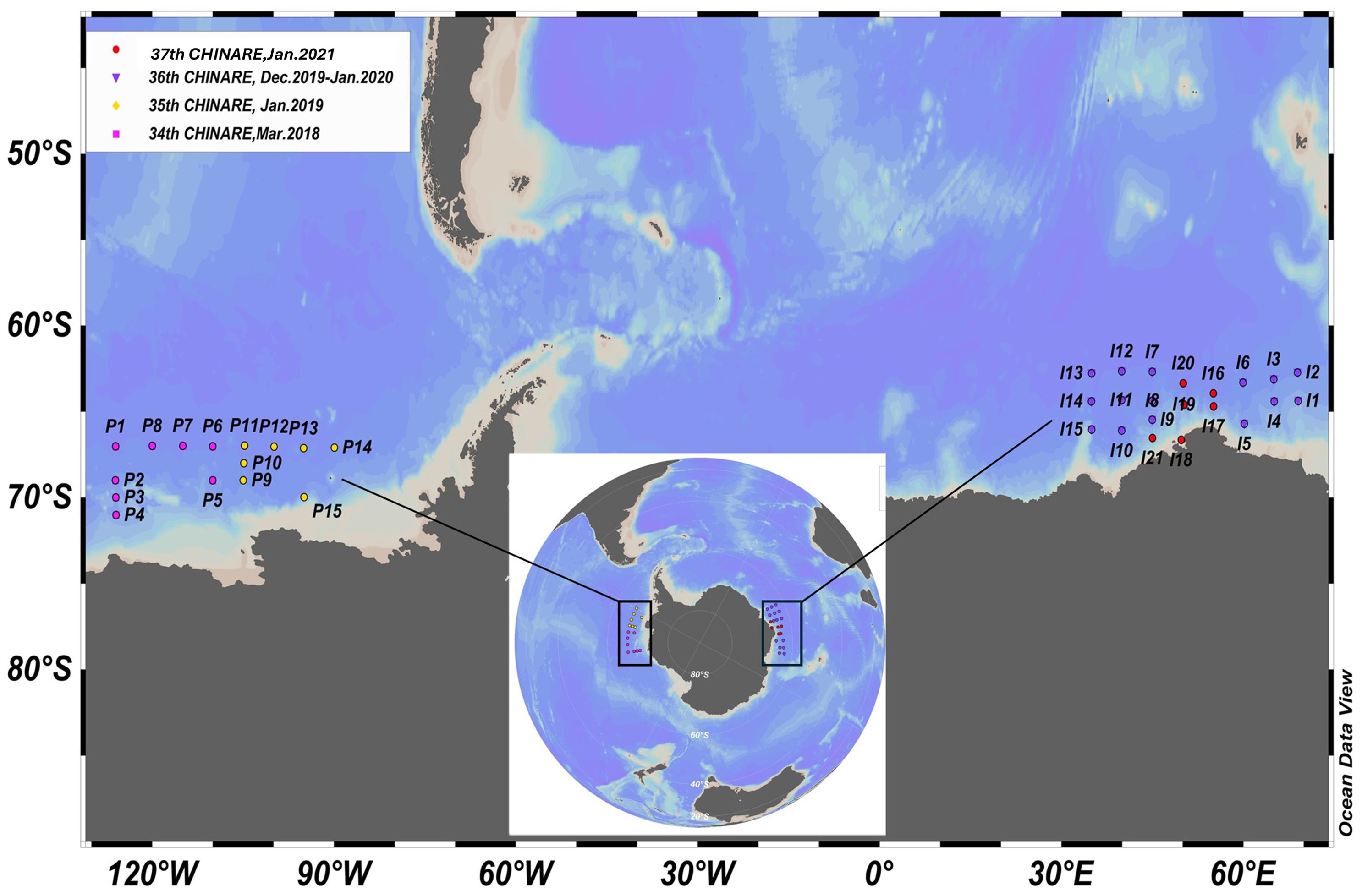
Figure 1. Sampling locations in the East-Pacific sector between 90 to 130 °W (station P1-P15) and the Indian sector between 30 to 70°E (station I1-I21).

2.2 Hydrography and water masses analysis

As potential physical drivers of zooplankton distribution, temperature, salinity, and dissolved oxygen patterns were exhibited by three-dimensional temperature, salinity and oxygen profiles by Python. Then, in-situ measurements of temperature and salinity were utilized to construct T-S diagrams and define water masses from 0-1500 m depth. AASW is characterized by temperatures ranging from −1.8 to 1.0 °C and salinity between 33.0 to 33.7 (Smith et al., 1999). Additionally, WW is located beneath AASW and can be identified by a temperature minimum of approximately −1.5 °C, with salinity between 33.8 to 34.0 (Smith et al., 1999). Circumpolar Deep Water (CDW) was defined by potential temperature lower than 1.5 °C and salinity between 34.5 to 34.75 thresholds, and modified CDW was identified as the water mass with temperature lower than 1.5 °C and salinity lower than 34.7 (Zu et al., 2022). Furthermore, as physical characteristics of water masses, these temperature and salinity ranges will be used in subsequent steps to identify any correlation between zooplankton abundance and water masses.

2.3 Zooplankton identification and counts

In the laboratory, zooplankton specimens were identified to the lowest possible taxonomic level based on morphological features of species or groups and were counted using a Nikon SMZ 745T dissecting microscope. A compound microscope was used to examine closely the minute taxonomic characteristics. Various identification manuals and marine copepod websites were used to aid in identifying the specimens (Kirkwood, 1982; O’Sullivan, 1982a, O’Sullivan, 1982b, O’Sullivan, 1983, O’Sullivan, 1986; Razouls et al., 2023). Macro-zooplankton (>2 mm in body length) were counted in each complete sample. For meso-zooplankton (200 μm-2 mm), sub-splits of 1/2 to 1/32 (depending on the numerical density of individuals) of the complete sample were obtained using a Folsom plankton splitter, ensuring a minimum of 500 individuals per sample was counted. Additionally, four dominant calanoid copepod species (Calanoides acutus, Calanus propinquus, Metridia gerlachei, and Rhincalanus gigas) and Euphausiacea (in the genera Euphausia and Thysanoessa) were identified to adult, subadult, and copepodite stages. These different stages were totalled per species for analysing species abundance. Then, species abundance in each stratum was calculated by dividing counts of individuals by the volume of water filtered by each net. Finally, zooplankton average abundance in each stratum of each sector was calculated and visualized using Python.

2.4 Zooplankton cluster analysis

Zooplankton community structure was analysed using PRIMER version 6 and Python. To preprocess input data, zooplankton abundance data from 36 stations were fourth root-transformed to ensure influence from rarer species and down-weight the influence of abundant species (Quinn and Keough, 2002). The different life stages of the common copepods and Euphausiacea were analysed as separate components in the cluster analysis. To avoid potential effects caused by the diel vertical migration of zooplankton on community structure, all zooplankton samples in each sector were classified as daytime samples and nighttime samples based on local sunset and sunrise times (https://gml.noaa.gov/grad/solcalc/sunrise.html) in each sector and used three-way AMOSIM (sampling layers, sampling years and months, and sampling time) to test the effects of different sampling time (day or night). Subsequently, data from the East-Pacific sector and Indian sector were separately subjected to cluster, ANOSIM, and SIMPER (similarity percentage) analyses. To segregate the zooplankton into communities, the transformed data were used in a q-type cluster analysis based on the Bray-Curtis dissimilarity index and group-average linkage classification. Additionally, all cluster groups were visualized by PRIMER. Following this, ANOSIM was conducted to test for similarity within each resultant community (cluster), and identify the most significant sampling factors, such as water layer and sampling year and month. The cluster groups were treated to the SIMPER analysis to determine which species significantly contributed to the similarity within and between clusters. Finally, the proportion of the most abundance taxa that largely contribute to zooplankton clusters were illustrated by stacked bar chart using Python.

2.5 The environmental drivers on zooplankton abundance

To improve understanding of the environmental factors influencing zooplankton abundance, the relationships between temperature, salinity, oxygen, and zooplankton abundance were evaluated independently using Generalized Additive Models (GAMs) in R Studio (version 4.21). Average values of salinity, temperature, dissolved oxygen, and zooplankton abundance were calculated for each sampling stratum (0-100, 100-200, 200-500, 500-1000, 1000-1500 m) at fifteen stations in the East-Pacific sector and ten stations in the Indian sector. Data from other 11 stations (I5-I15) in the Indian sector were not analysed due to the lack of CTD data. To examine the relationships between zooplankton abundance and water masses further, we categorized zooplankton into three groups: ‘highest abundance’ (upper 90^th percentile), ‘medium abundance’ (45^th to 55^th percentile), and ‘lowest abundance’ (lower 10^th percentile). GAMs were used to forecast the ranges of temperature, salinity, and dissolved oxygen corresponding to these three zooplankton abundance categories within each sector. We then tested whether these predicted temperature and salinity ranges correlated with specific water masses. For the analysis of chl-a concentration and zooplankton abundance, we used the average chl-a concentration at each station from the surface layer (0-200 m), where phytoplankton primarily grow, and the overall zooplankton abundance at each station from 0 to 1500 m for both sectors. We included deep layer zooplankton abundance into overall abundance because deep ocean zooplankton productivity is positively related to surface layer primary production in the global ocean (Hernández-León et al., 2020). Given the short turnover time of phytoplankton cells (chl-a concentration) and their rapid concentration changes, we also utilized monthly Aqua-MODIS satellite chl-a concentration data from NASA Ocean Color to verify phytoplankton phenology and changes during the sampling months (as shown in Supplementary Figures 1, 2). This approach aimed to mitigate the potential effects of different sampling years and months.

3 Results

3.1 Hydrographic features and water masses

Environmental conditions including temperature, salinity, and dissolved oxygen had similar ranges between stations in the two sectors and exhibited similar patterns vertically from surface to 1500 m (Figure 2). Salinity ranged from 32.5 to 34.8 at different stations; additionally, it increased with depth and stabilized from around 500 to 1500 m (Figure 2). Dissolved oxygen levels generally decreased from the surface to depth ranging from 11 to 5 mg. L^-1. Ocean temperature, ranging from -1.7 to 2.1 °C at different stations, was low at around 0-200 m, peaked at approximately 500 m, and then slightly decreased from 500 to 1500 m (Figure 2). Chl-a, as a most important biotic variable, was primarily distributed in the top 200 m layer. The average depth-integrated chl-a concentration varied between stations, ranging from 0.12 to 1.87 mg. m^-³. The average chl-a concentrations in the 0-200 m layer in Mar 2018 and Jan 2019 in the East-Pacific sector (0.21 mg. m^-3) were lower than those in the Indian sector (0.39 mg. m^-3), measured in Dec 2019-Jan 2020 and Jan 2021.

Figure 2

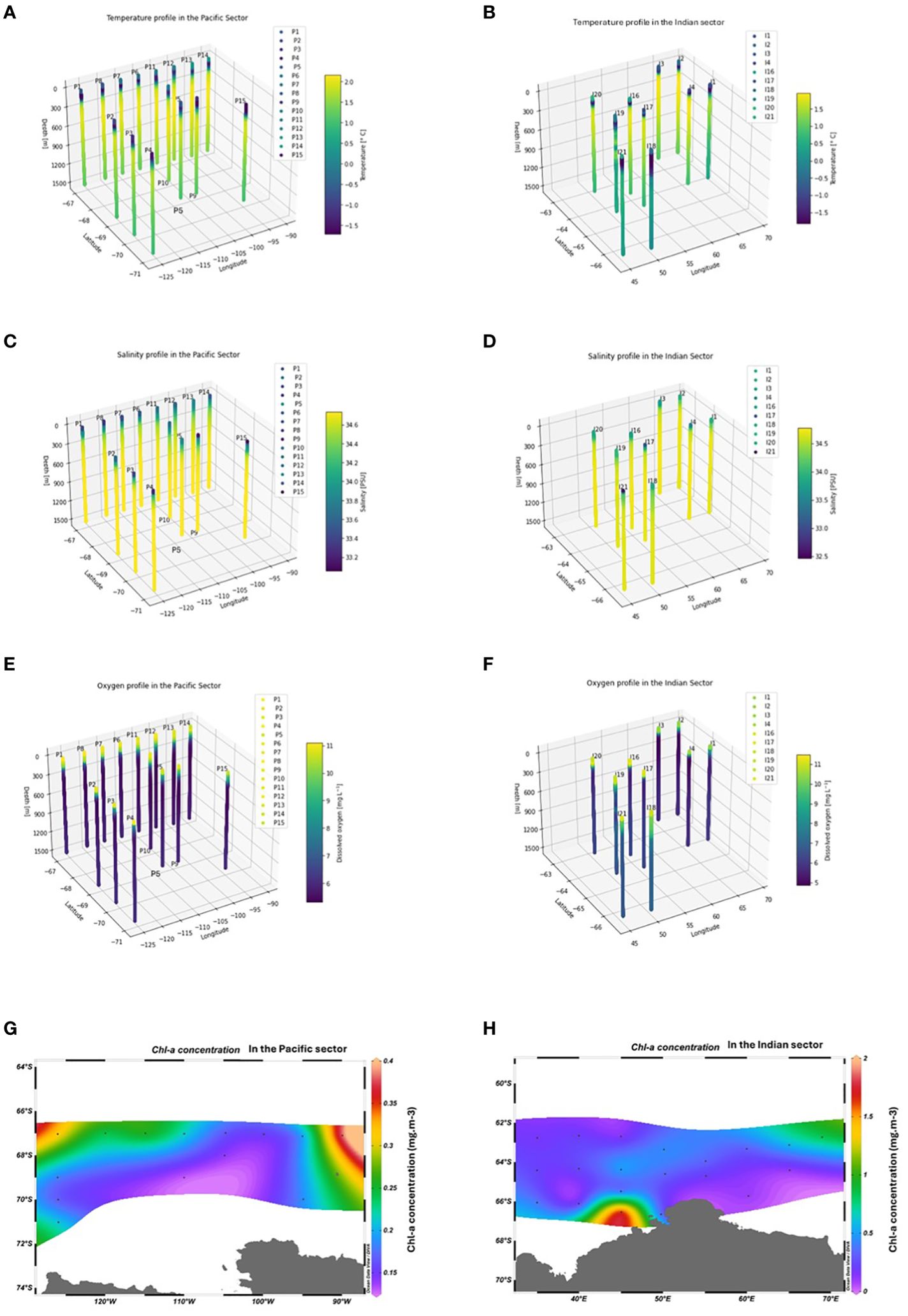
Figure 2. The three-dimensional temperature, salinity, dissolved oxygen profiles of each station from 0-1500m in the East-Pacific and Indian sectors of the Southern Ocean subplot (A–F). The average phytoplankton concentration in each sector (G, H).

The distribution of water masses was generally similar between the two sectors. In the East-Pacific sector (90-130 °W), three water masses were identified: AASW, WW, and CDW (Figure 3). AASW, with its relatively fresh water (salinity <33.8) and temperature, ranging from -1.5 to 0.5 °C, was found on the surface. WW characterized by higher salinity (33.8-34.3) and the lowest temperature (<-1 °C) lay beneath the AASW. CDW was found underneath WW, spanning approximately down to the upper bathypelagic layer, and had the highest temperature (1.5-2 °C) and highest salinity (34.4-34.75). In the Indian sector (30-70 °E), the same water masses as those in the East-Pacific sector, including AASW, WW, and CDW, were identified based on the T-S diagram shown in Figure 3. Modified CDW, characterized by lower temperature (<1.5 °C) and lower salinity (<34.7) than typical CDW, was found exclusively in the Indian sector (Figure 3).

Figure 3

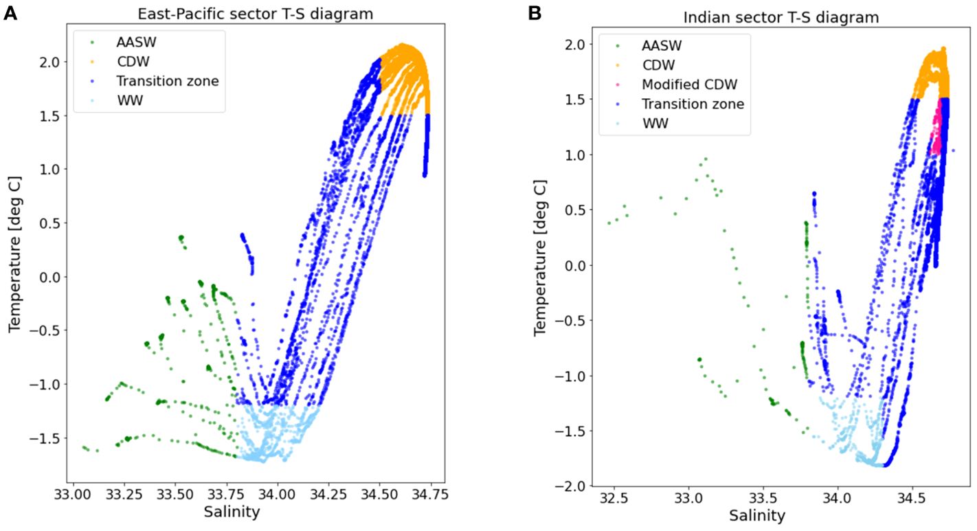
Figure 3. The T-S (Temperature to salinity) diagram showing distribution of the Antarctic Surface Water (ASW), Winter Water (WW), Circumpolar Deep Water (CDW), modified CDW and transition zone from 0 to 1500 m in the East-Pacific (A) and Indian sectors (B). The temperature and salinity data in each sector were collected on different years and months. Data were collected in March 2018 and January 2019 in the East-Pacific sector and Dec 2019 to Jan 2020 and Jan 2021 in the Indian sector respectively.

3.2 Zooplankton diversity

Sixty-three taxa belonging to nine mesozooplankton groups were found in the two sectors (Table 1; Supplementary Table 2). These include Copepoda, Euphausiacea, Chaetognatha, Polychaeta, Amphipoda, Tunicata, Pteropoda, Ostracoda, and Cnidaria (Table 1). Taxonomic diversity was fifty-six taxa in the Indian sector and forty taxa in the East-Pacific sector across different years and months (Table 1). Copepods represented 53% of zooplankton diversity in the East-Pacific sector and 57% of zooplankton diversity in the Indian sector. Differences in species composition were largely attributed to variations among copepods. For instance, Calanus simillimus, Microcalanus pygmaeus, Aetideopsis antarctica, Racovitzanus antarcticus, Stephos longipes and Bathycalanus bradyi were only found in the Indian sector, whereas Bathycalanus richardi, and Farrania frigida were only collected in the East-Pacific sector, though these latter species were collected infrequently. For macro-zooplankton taxa (> 2 mm), Euphausia superba and Thysanoessa macrura were commonly found in both sectors but these species were likely underestimated due to avoidance of the Hydro-Bios multinet (Atkinson et al., 2012). Gelatinous taxa, such as salps, were absent in 28 out of 36 stations, and had low abundance in the samples. Chaetognaths such as Eukrohnia hamata and Pseudosagitta gazellae were abundant in the surface layer at some stations, although many specimens could only be identified to the phylum Chaetognatha due to damage to or disappearance of their lateral fins and heads, both of which are diagnostic features. For other common taxa, such as Polychaeta, Pteropoda, and Cnidaria, only a few specimens were found in the samples, and they were only infrequently observed.

Table 1

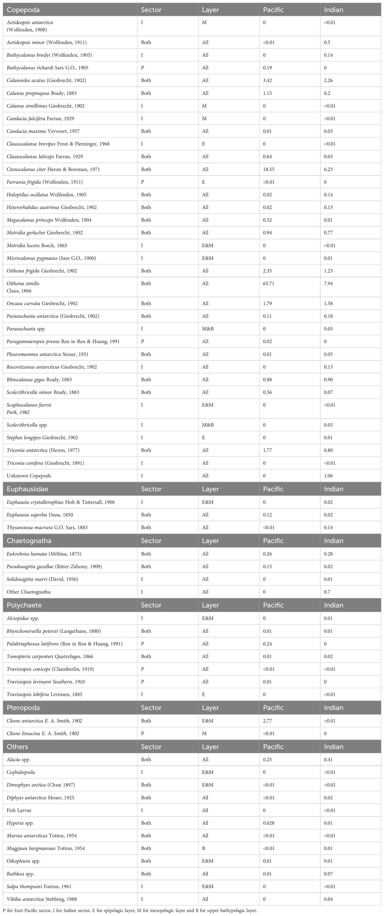
Table 1. Zooplankton diversity in the East-Pacific and Indian sectors, and three layers, as well as average zooplankton abundance for each species in the two sectors.

Taxonomic diversity was higher in the 0-200 m layer, known as epipelagic layer, and the mesopelagic layer (500-1000 m) in the two sectors (Table 1). Additionally, diversity was lowest in the top 500 m of the bathypelagic layer, between 1000-1500 m (Table 1). The most common species could be found throughout the water column, down to 1500 m. In the epipelagic layer, fifty-five taxa were found, including a large proportion of common copepods such as C. citer and O. similis. In the 200-1000 m layer, as known as the mesopelagic layer, some copepods, such as A. antarctica (meso- to bathypelagic species), and Scolecithricella spp., which were absent from surface layers in the samples, were found. The upper bathypelagic layer had the lowest diversity (forty-four taxa). Species such as Oikopleura spp., Salpa thompsoni, Clione antarctica, and Clione limacina were rare or absent in deep layers, although they were abundant in the surface layers of a few stations.

3.3 Zooplankton abundance between layers in each sector

Zooplankton abundance was variable between water layers and sectors. Zooplankton abundance peaked in the epipelagic layer and subsequently declined with each successive water layer at each station (Figure 4). The average abundance was significantly higher in the East-Pacific sector (100 individual.m^-3) than in the Indian sector (27 individual.m^-3) (Figure 4). The elevated zooplankton abundance in the East-Pacific sector was predominantly due to a higher abundance of small common copepods such as O. similis, O. frigida, O. curvata, T. antarctica, and C. citer in the epi-pelagic layer. In our samples, these small copepods dominated numerically in most meso-zooplankton (0.2-20 mm) communities. Four large calanoids, including C. acutus, C. propinquus, M. gerlachei, and R. gigas were also abundant, including abundant copepodite stages of these calanoids were present in the surface layer.

Figure 4

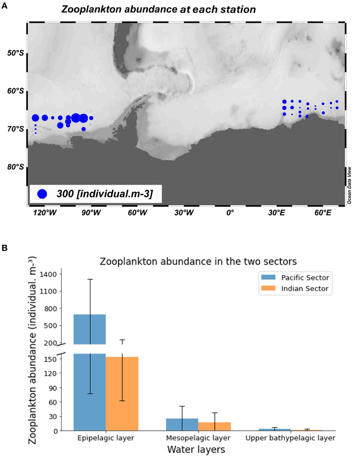
Figure 4. Average zooplankton abundance for each station subplot (A) and average zooplankton abundance in five continuous zooplankton sampling strata in the East-Pacific sector (Mar 2018 and Jan 2019) and the Indian sector (Dec 2019-Jan 2020 and Jan 2021) subplot (B).

3.4 The community structure of zooplankton

In the East-Pacific sector, five communities were identified by cluster analysis (Figure 5). Copepods numerically dominated all the meso-zooplankton communities, while communities in deeper layers had a higher proportion of non-copepod groups including Ostracoda, Chaetognatha and Amphipoda. Three larger communities (C, D, E) were broadly defined by ocean stratification, encompassing the epi-pelagic layer and deeper layers (200-1500m) (Figure 5). Cluster E consisted of zooplankton from the epipelagic layer, displaying a similarity of 50% (Figure 5). The epi-pelagic community (cluster E) was characterized by the highest average zooplankton abundance (796 individual. m^-³) and the highest composition of common copepod Oithona similis (66%) in total abundance (Figure 6). Pteropoda were the most abundant non-copepod group, representing 3% of total abundance. Other zooplankton taxonomic groups, including Chaetognatha, Amphipoda, Tunicata, and Cnidaria, contributed less than 1% of the total abundance. Cluster D, with a similarity of 54%, comprised zooplankton from the deeper layers between 200-1500 m, excluding samples P3(2), P4(2), and P15(2) from the 100-200 m layer (Figure 6). In cluster D, copepods were also the most abundant group, making up 92% of total abundance (Figure 6). The O. similis, C. citer, Oithona frigida had more evenly distribution. Moreover, Chaetognatha, Ostracoda, and Amphipoda were the most abundant non-copepod taxa, constituting 3%, 2.4%, and 1.6% of the total abundance, respectively (Figure 6). Cluster C, with an average similarity of 51%, included the zooplankton communities mainly collected in the upper bathypelagic layer in May 2018. In cluster C, Amphipoda represented 11% of total abundance behind common copepods. The other two minor communities (A and B) mainly consisted of zooplankton from 500-1500 m layers. Cluster A, with similarity of 62%, and cluster B, with similarity of 64%, mainly consisted of copepod. Moreover, the highest proportion of Chaetognatha (14%) and Ctenocalanus citer (33%) were recorded in cluster A and cluster B respectively.

Figure 5

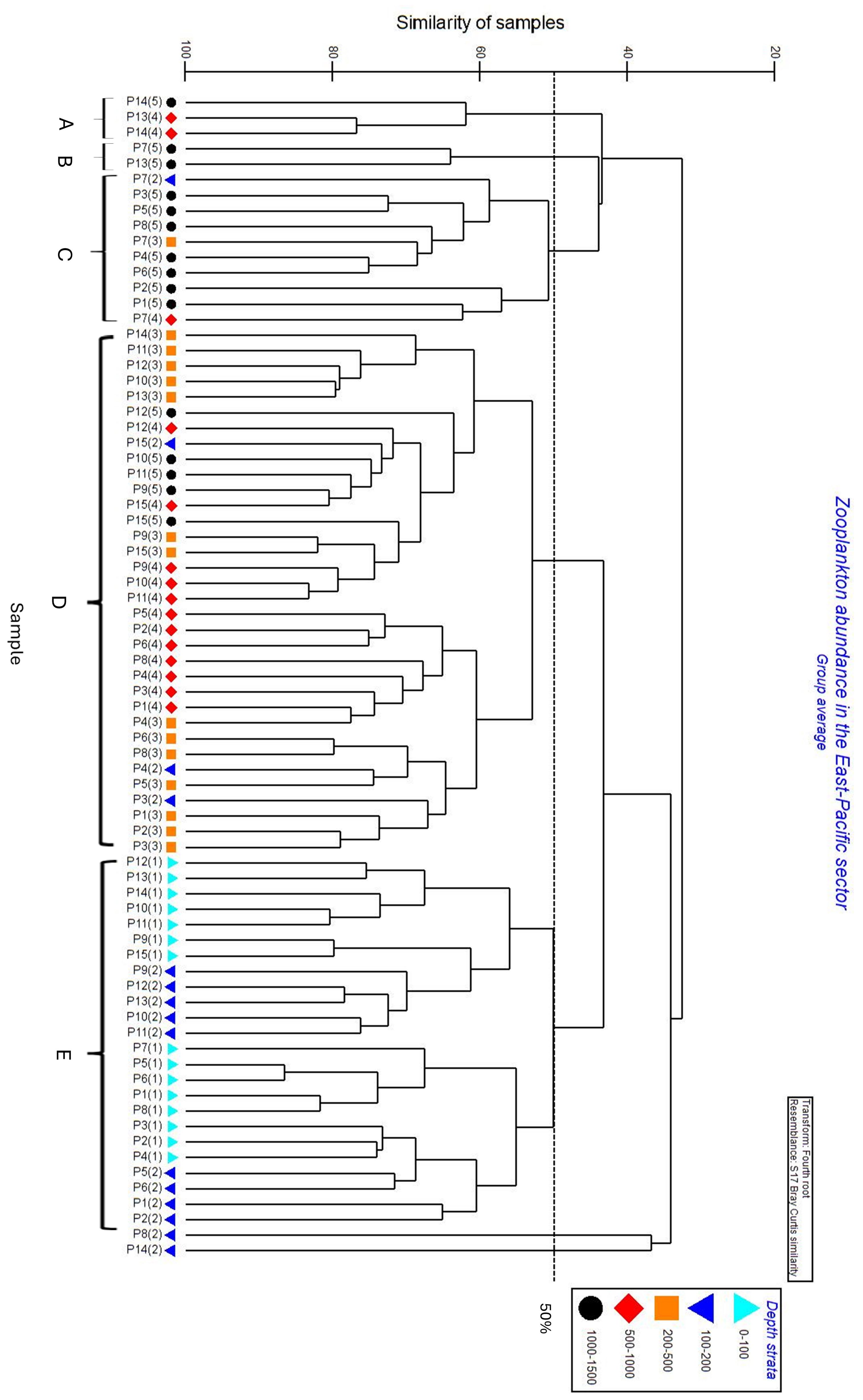
Figure 5. Cluster analysis of zooplankton assemblages in the East-Pacific sector between 90-130°W from 0-1500m with five continuous zooplankton sampling strata [0-100 m: (1), 100-200 m: (2), 200-500 m: (3), 500-1000 m: (4) and 1000-1500 m: (5)].

Figure 6

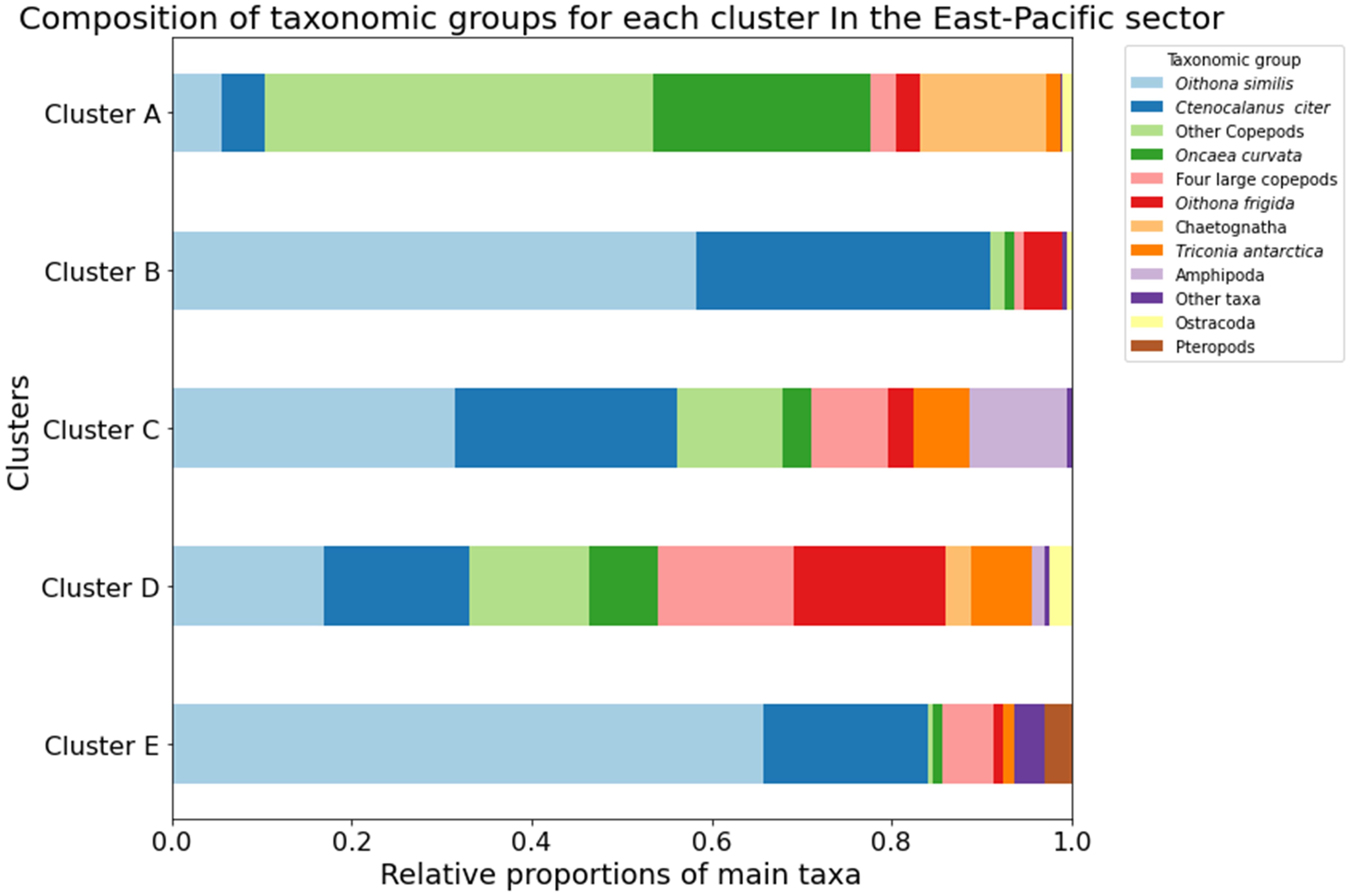
Figure 6. The proportion of most abundant meso-zooplankton taxa and species in zooplankton communities in the East-Pacific sector Cluster A–E.

In the Indian sector, four clusters were primarily distinguished based on water layers (Figure 7). Copepods dominated the mesozooplankton communities, representing 81% to 96% of total abundance (Figure 8). Cluster F, with an average similarity of 50%, comprised zooplankton from the epipelagic layer. In this epipelagic community, O. similis (40%) and C. citer (30%) were still numerically dominant. Non-copepods group including Chaetognatha (3.1%) made a small contribution to this community (Figure 8). Clusters G, with a similarity of 57% and H, with a similarity of approximately 50%, encompassed zooplankton collected in the 200-1500 m strata. These deeper layer communities had an increased proportion of non-copepods taxa such as Chaetognatha (14% and 6% respectively). Nonetheless, copepod taxa, especially Paraeuchaeta sp., were one of the most abundant species. Cluster I, with an average similarity of 60%, mainly included the zooplankton community in the 500-1500 m strata. In this community, four large calanoid copepods (C. acutus, C. propinquus, M. gerlachei, and R. gigas), and cyclopoids such as O. frigida (12%) and O. curvata (15%) made up a significant proportion; additionally, Ostracoda and Chaetognatha represented 5% and 7% of the total abundance (Figure 8).

Figure 7

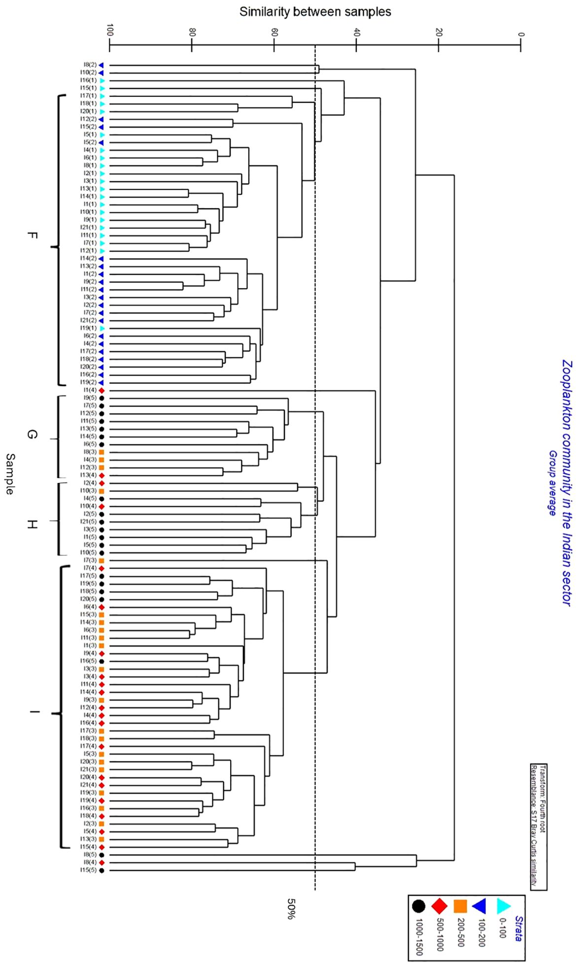
Figure 7. Cluster analysis of zooplankton assemblages in the Indian sector between 30-70°E from 0-1500m with five continuous zooplankton sampling strata.

Figure 8

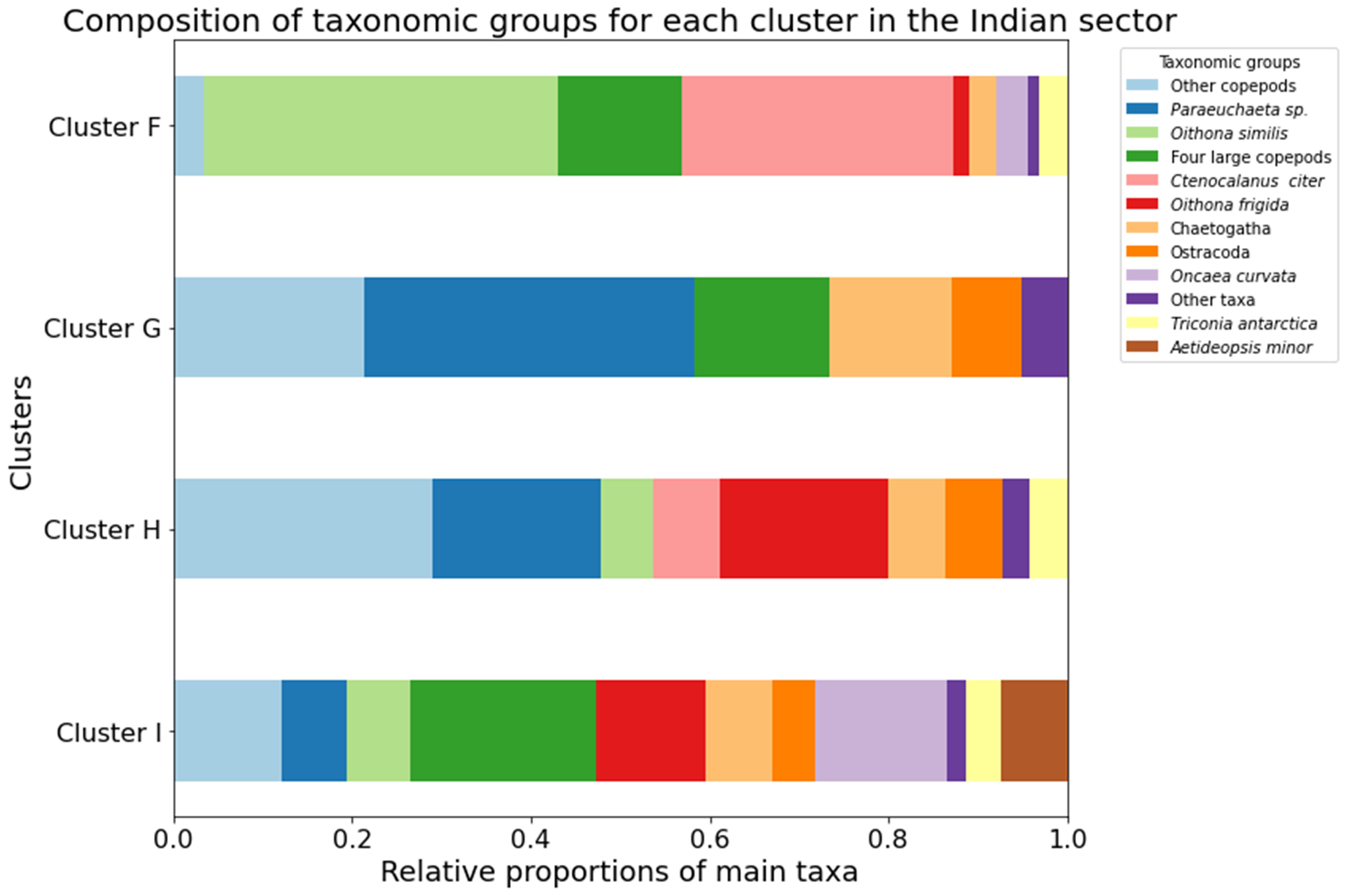
Figure 8. The proportion of most abundant meso-zooplankton taxa and species in zooplankton communities in the Indian sectors (Cluster F–I).

3.5 Environmental drivers on zooplankton abundance and communities

Based on the two-ways ANOSIM, there was no significant difference between daytime and nighttime zooplankton data (R=0.2 for East-Pacific sector, and R=-0.1 for Indian sector), so the zooplankton abundance data was subsequently analysed regardless of the sampling time. The water layer is a more important factor than sampling year and month to define a community in both sectors. In the Indian sector, water layer (R=0.69) was identified as the main factor defining a zooplankton community, rather than the sampling year and month (R=0.17). In the East-Pacific sector, where zooplankton samples were collected in May 2018 and January 2019, the water layer (R=0.49) played a slightly more significant role than sampling year and month (R=0.47).

In both sectors, GAMs exhibit non-linear patterns between zooplankton abundance and temperature, salinity, and oxygen across all water strata (Figure 9, Table 2). Three zooplankton abundance categories were correlated with specific ranges of temperature and salinity, corresponding to particular water masses. In the East-Pacific sector, the highest zooplankton abundance was associated with specific ranges of temperature (-1 to -0.6 °C) and salinity (33.6 to 33.7). Notably, these specific temperature, salinity, and oxygen ranges overlapped with the physical properties of AASW observed in the Pacific sector, when comparing the water masses analysis in Figure 3 and GAMs results in Figure 9. Medium zooplankton abundance was associated with intermediate temperature (0.1 to 0.4 °C) and salinity (34.1 to 34.2), which did not correlate with any specific water mass but indicated a transition zone. The lowest zooplankton abundance was associated with higher temperatures (1.1 to 1.5°C) and salinities (34.5 to 34.6), corresponding to CDW (Figures 3, 9).

Figure 9

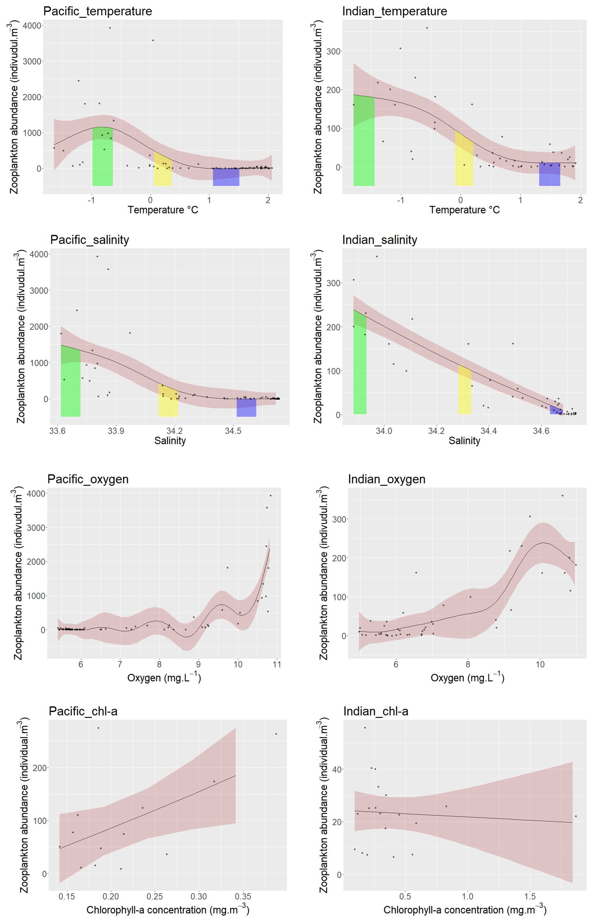
Figure 9. The relationships between salinity, temperature and dissolved oxygen and zooplankton abundance from five continuous sampling strata in the East-Pacific and Indian sectors, and the relationships between the chl-a concentration and zooplankton abundance for each station in the East-Pacific and Indian sector. Each curve represents the fitted relationship between zooplankton abundance and each parameter respectively. The pink shaded areas indicate the 95% confidence interval. The green, yellow, and purple shaded areas represent the upper 90^th, medium 45^th to 55^th, and lower 10^th percentiles of zooplankton abundance, along with their corresponding temperature, salinity, and oxygen ranges.

Table 2

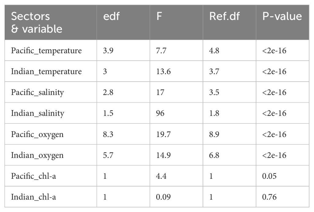
Table 2. GAMs results including Effective degrees of freedom (edf), F, Reference Degree of Freedom (Ref.df) and P-value between temperature, salinity, oxygen, chl-a and zooplankton abundance for each sector.

Similarly, in the Indian sector, the highest zooplankton abundance coincided with lower salinity (33.88 to 33.93) and the lowest temperatures (-1.8 to -1.4 °C), indicative of AASW (Figures 3, 9). Although the salinity range here is slightly higher than typical AASW (33.0 to 33.7), the salinity of AASW can measure up to 34.3 PSU (Carter et al., 2009). Medium zooplankton abundance was associated with intermediate temperature (-0.1 to 0.2 °C) and salinity (34.28 to 34.33), consistent with the transition zone’s physical properties (Figures 3, 9). The lowest zooplankton abundance corresponded to the highest temperatures (1.3 to 1.7 °C) and salinities (34.63 to 34.68), overlapping with CDW in the Indian sector (Figures 3, 9). The results from GAM also revealed that chl-a concentration showed a positive relationship with zooplankton abundance in the East-Pacific sector but a non-significant relationship in the Indian sector (Figure 9, Table 2). Furthermore, the East-Pacific sector exhibited higher zooplankton abundance and lower chl-a concentrations in March 2018 and January 2019. In contrast, the Indian sector showed significantly higher chl-a concentration and lower zooplankton abundance in December-January of 2020 and January 2021.

4 Discussion

4.1 Comparing zooplankton diversity, abundance and communities between two sectors

All sixty-three taxa in our samples are commonly found in the Southern Ocean (Kirkwood, 1982; O’Sullivan, 1982a, O’Sullivan, 1982b, O’Sullivan, 1983, O’Sullivan, 1986; Ward et al., 2003, Ward et al., 2014a; Razouls et al., 2023). Zooplankton taxonomic diversity in our surveys is slightly lower compared to other observations (Atkinson and Sinclair, 2000; Nicol et al., 2010; Flores et al., 2014; Ward et al., 2014a; Yang et al., 2017). This is partly because of some fragmented or unknown jellyfish, Chaetognatha, copepod larvae and Cephalopoda being classified only as indetermined species or into Class level, which reduces the estimated species diversity. Some species, such as C. brevipes, M. princeps, and Candacia falcifera, that were only collected in the epipelagic layer or meso to bathypelagic layers, are restricted to these layers; however, others, including C. simillimus and A. antarctica, which were only collected in the mesopelagic layer, have a wider distribution from the epipelagic to mesopelagic layers (Razouls et al., 2023). For meso-zooplankton diversity in each sector, most species, including M. pygmaeus, A. antarctica, R. antarcticus, S. longipes and B. bradyi and B. richardi, that were only found in one sector by our survey are actually circumpolar species (Razouls et al., 2023). As a result, the in-situ diversity might be similar in the two sectors. The similarity in zooplankton diversity between the East-Pacific and Indian sectors aligns with previous findings of consistent taxonomic composition of Antarctic meso-zooplankton communities across the circumpolar region (Dubischar et al., 2002; Pinkerton et al., 2020; Takahashi and Hosie, 2020; Johnston et al., 2022).

Zooplankton abundance varies across sectors and layers (Wilson et al., 2015; Stevens et al., 2015; Pakhomov et al., 2020; Dietrich et al., 2021). Our results reveal that zooplankton abundance in the deeper layers is generally an order of magnitude lower than the epi-pelagic assemblages. Moreover, the cluster analysis results revealed that zooplankton communities were generally divided by water layers. This finding is consistent with previous surveys in the various regions including Prydz Bay, the Scotia Sea, Drake Passage and the Polar Front (Atkinson and Sinclair, 2000; Ward et al., 2003; Flores et al., 2014; Ward et al., 2014a; Yang et al., 2017; Pinkerton et al., 2020). Our results also showed that zooplankton abundance was more than three times higher in the East-Pacific sector than in the Indian sector. There is little evidence showing significant higher zooplankton abundance between 90-130°W in the East-Pacific sector than between 30-70°E in the Indian sector by previous studies (Pakhomov and McQuaid, 1996; Atkinson et al., 2012; Venkataramana et al., 2020). As a result, this higher abundance may be partially influenced by variation in monthly and annual zooplankton population dynamics (Atkinson et al., 2012). Our ANOSIM analysis also highlighted the secondary roles of sampling years and months in regulating zooplankton communities. Previous studies have also found that the abundance of dominant calanoid copepods peaks in late summer in various regions of the Southern Ocean (Atkinson et al., 1997; Schnack-Schiel and Isla, 2005; Hunt and Hosie, 2006). Consequently, zooplankton abundance in the Indian sector may not have reached its peak between December to January, leading to underestimation (Takahashi and Hosie, 2020), when we were comparing zooplankton abundance between these two sectors.

Zooplankton community structure varied in each layer and sector, the dominant species in meso-zooplankton assemblages in the epipelagic and mesopelagic layers are consistently similar respectively in both sectors. These include calanoid species such as C. acutus, C. propinquus, M. gerlachei, C. citer, and R. gigas as well as smaller cyclopoid species including O. similis and O. curvata. These copepods account for more than 75% of total biomass in both our study and in previous observations (Atkinson et al., 2012). Other less abundant taxa, encompassing salps, Amphipoda, Polychaeta, and Chaetognatha, generally exhibit uneven proportions across different sectors in the Southern Ocean (Ward et al., 2003; Swadling et al., 2010; Pinkerton et al., 2020). As another dominant species in the Southern Ocean, Antarctic krill (Euphausia superba) may be underestimated by their net avoiding behaviour (Atkinson et al., 2012).

4.2 Influence of physical drivers especially water masses on zooplankton distribution in different layers and the two sectors

Water masses play a crucial role in regulating zooplankton communities across different regions of the Southern Ocean (Swadling et al., 2010; Marrari et al., 2011; Mańko et al., 2020). Our GAM model results showed that the most abundant zooplankton assemblages in both sectors were related to specific temperature and salinity ranges, aligning with the physical properties of the AASW, while the lowest zooplankton abundance corresponded to the physical properties of the CDW. These specific temperature and salinity ranges are best understood qualitatively rather than as precise predictors of zooplankton abundance. These results establish a correspondence between water masses and zooplankton abundance, highlighting the impacts of AASW and CDW on the highest and lowest zooplankton abundances, respectively. Comparing with previous studies, acoustic surveys have also demonstrated different zooplankton assemblages associated with AASW and upper CDW respectively in coastal regions of the Southern Ocean (Lawson et al., 2004; Marrari et al., 2011). This implies that not only temperature, salinity, and oxygen themselves (Hunt et al., 2016), but also the combined physical and biological properties of AASW might have a critical effect on zooplankton abundance. Specifically, AASW, with its highest dissolved oxygen content and lower salinity and temperature, may provide a preferred environment for epipelagic zooplankton during the summer, although the thermal and salinity tolerances, as well as oxygen consumption of Antarctic zooplankton, are not well studied (Atkinson et al., 2012; Costa et al., 2021). Moreover, the highest concentration of food sources, such as phytoplankton cells, in the AASW tends to attract zooplankton and Euphausiacea swarms (Tarling and Fielding, 2016; Pauli et al., 2021). In deeper water masses, CDW with its lowest oxygen levels and food availability (Bindoff et al., 2000; Carter et al., 2008; Williams et al., 2010; Carter et al., 2012) could shape distinct zooplankton communities with lowest zooplankton abundance.

4.3 Biotic drivers including chl-a concentration on zooplankton community structure in both sectors

The difference in zooplankton abundance vertically could be affected by biotic factors such as chl-a concentration. As secondary producers, zooplankton abundance is also influenced by primary production, which is largely determined by chl-a concentration, a process known as bottom-up control (Hernández-León et al., 2020). Our observational data in the East-Pacific sector coincides with bottom-up control. However, the Indian sector showed non-significant relationship between zooplankton abundance and in-situ chl-a concentration. Moreover, the Indian sector had higher phytoplankton concentration but lower zooplankton abundance comparing with East-Pacific sector. These opposite results implicate the phenology of phytoplankton and zooplankton. For instance, in-situ chl-a concentration is generally higher in early summer between December to January, but zooplankton abundance reaches its peak in late summer in the high latitude of the Southern Ocean (Atkinson et al., 1997; Atkinson, 1988a; Schnack-Schiel and Isla, 2005; Hunt and Hosie, 2006; Wright et al., 2010; Takahashi and Hosie, 2020). NASA satellite data on chlorophyll-a (chl-a) concentrations supports our inference regarding phytoplankton phenology. In the East-Pacific sector, the average chl-a concentration decreased to 0.25 mg. m³ in March 2018 (the sampling month during the 34th CHINARE) from higher values in early summer (0.43 mg.m³ in December 2017 and 0.32 mg/m³ in January 2018), as shown in Supplementary Figure 1. In the Indian sector, chl-a concentrations were higher in early summer, between December and January (our sampling months during the 36th and 37th CHINARE), compared to late summer, from February to March, as indicated in Supplementary Figure 2. For zooplankton abundance, small copepods including O. similis, C. citer and O. curvata, were important contributors to higher total abundance in the East-Pacific sector. However, many of these small herbivorous and omnivorous copepods reproduce during spring and early summer, but their early life stages are often too small to be effectively collected by nets with a mesh size of 200 µm during 36 and 37^th CHINARE (Hagen, 1999; Ward and Hirst, 2007; Atkinson et al., 2012; Cornwell et al., 2020). Consequently, the chl-a concentration played important roles in regulating zooplankton abundance, but the underestimated contribution of small copepod larvae to total zooplankton abundance and peaked chl-a concentration in early summer may complicate the existing understanding of relationships between zooplankton abundance and chl-a concentration in the Indian sector.

The vertical distribution of zooplankton, including their abundance and community composition, is also consistent with their diet and food availability in each layer. In the surface layer, the proportion and abundance of copepods were highest than deeper layers. This coincides with the highest food availability, such as highest concentration of chl-a for grazers in the surface layer. For example, the most numerous taxa, including O. similis, O. curvata, C. citer, and O. frigida, as well as C. acutus and C. propinquus in the epipelagic layer in our sample, are either herbivorous or omnivorous (Kattner et al., 2003; Pond and Ward, 2011). Moreover, our observations and other studies have shown that the copepodite stages of calanoids, such as C. acutus and C. propinquus, concentrate in the epipelagic layer for ontogenetic development during summer (Conroy et al., 2020). In deeper layers, the reduction in phytoplankton cells but increases in sinking particles could benefit omnivores, scavengers, or predators such as Chaetognatha and Amphipoda (Nishikawa and Tsuda, 2001; Proud et al., 2017). In our samples, the relative proportions of the herbivorous and omnivorous copepods, including O. similis, O. curvata, C. citer, and O. frigida, C. acutus and C. propinquus, decreased in the deeper layers. However, the relative proportions of Amphipoda, Chaetognatha, and Ostracoda increased in the deeper layers in both sectors. Based on existing fatty acid and stable isotope analysis, these groups, including Hyperiidae, Gammaridae, E. hamata, P. gazellae, and Alacia spp. are generally considered to be either carnivores or omnivores (Øresland, 1990; Froneman and Pakhomov, 1998; Nelson et al., 2001; Kruse et al., 2010). The increased relative proportions of carnivores and omnivores in deeper layers align with previous observations that zooplankton trophic levels generally increase with depth (Hernández-León et al., 2020). When considering the combined effects of primary production, food availability and physical water mass properties on zooplankton abundance, the decrease in zooplankton abundance with increasing depth and water masses may be attributed to reduced food availability and unfavourable physical conditions, such as low oxygen levels, in deeper water masses.

Diel vertical migration of zooplankton between the surface and deeper layers potentially affects their vertical distribution. However, our samples were collected upon the vessel’s arrival at each station, irrespective of the time of day, so these samples are not ideal and designed for analysis vertical migration between layers. Moreover, this migratory behaviour was not clearly observed and recorded in our study, perhaps due to the shorter migration distances caused by longer photoperiods during the sampling periods and low predatory pressure from visual mesozooplankton predators in the high latitude of the Southern Ocean (Pinkerton et al., 2010; Saunders et al., 2019; Conroy et al., 2020; Cao et al., 2022; Li et al., 2022).

5 Conclusions

The mesozooplankton community composition and dominant taxa in each layer between the East-Pacific and Indian sectors were similar during Austral summer between 2018 to 2021. However, zooplankton abundance varies across different sectors and declines significantly with three water layers. Our study integrated the common environmental drivers, including temperature and salinity, and chl-a concentration, into physical and biological characteristics of different water masses, and demonstrated that water masses that combined all these characteristic play significant roles in regulating vertical distribution of zooplankton in terms of abundance and composition in both sectors. These multiple environmental drivers provide new insights for understanding large-scale zooplankton abundance and distribution in the Southern Ocean, thereby enhancing our ability to analyse and quantify their ecological and biogeochemical roles and the impacts of climate changes on zooplankton community (Fraser et al., 2018). However, the detailed mechanisms of how some physical properties and movement of water masses influence zooplankton physiology, advection, and dispersal, and therefore their distribution, remain beyond the scope of this paper. Future research might integrate water mass dynamics, physiological analysis of zooplankton, and acoustic zooplankton data to deepen our comprehension of the mechanisms driving large scale zooplankton distribution horizontally and vertically.

Data availability statement

The original contributions presented in the study are included in the article/Supplementary Material. Further inquiries can be directed to the corresponding author.

Ethics statement

The manuscript presents research on animals that do not require ethical approval for their study.

Author contributions

YL: Conceptualization, Data curation, Formal analysis, Methodology, Software, Visualization, Writing – original draft, Writing – review & editing. YW: Data curation, Writing – review & editing. YS: Data curation, Writing – review & editing. GY: Conceptualization, Funding acquisition, Methodology, Project administration, Resources, Supervision, Writing – review & editing. KS: Methodology, Resources, Supervision, Writing – review & editing, Conceptualization.

Funding

The author(s) declare financial support was received for the research, authorship, and/or publication of this article. This work was supported by the National Natural Science Foundation of China (42276238), Impact and Response of Antarctic Seas to Climate Change (IRASCC-01-02-01D) and the Tai Shan Scholars Program.

Acknowledgments

We would like to thank the crew on R/V Xue long and Xue long 2 for their assistance with the plankton sampling and Polar Research Institute of China (https://www.pric.org.cn/) for providing temperature and salinity data.

Conflict of interest

The authors declare that the research was conducted in the absence of any commercial or financial relationships that could be construed as a potential conflict of interest.

Publisher’s note

All claims expressed in this article are solely those of the authors and do not necessarily represent those of their affiliated organizations, or those of the publisher, the editors and the reviewers. Any product that may be evaluated in this article, or claim that may be made by its manufacturer, is not guaranteed or endorsed by the publisher.

Supplementary material

The Supplementary Material for this article can be found online at: https://www.frontiersin.org/articles/10.3389/fmars.2024.1274582/full#supplementary-material

References

Abelmann A., Gersonde R., Knorr G., Zhang X., Chapligin B., Maier E., et al. (2015). The seasonal sea-ice zone in the glacial Southern Ocean as a carbon sink. Nat. Commun. 6, 8136. doi: 10.1038/ncomms9136

PubMed Abstract | Crossref Full Text | Google Scholar

Arrigo K. R., Thomas D. N. (2004). Large scale importance of sea ice biology in the Southern Ocean. Antarct. Sci. 16, 471–486. doi: 10.1017/S0954102004002263

Crossref Full Text | Google Scholar

Arrigo K. R., van Dijken G. L., Bushinsky S. (2008). Primary production in the Southern Ocean –2006. J. Geophys. Res. 113, C08004. doi: 10.1029/2007JC004551

Crossref Full Text | Google Scholar

Atkinson A. (1998a). Life cycle strategies of epipelagic copepods in the Southern Ocean. J. Mar. Syst. 15, 289–311. doi: 10.1016/S0924-7963(97)00081-X

Crossref Full Text | Google Scholar

Atkinson A., Peck J. M. (1988b). A summer-winter comparison of zooplankton in the oceanic area Around South Georgia. Polar Biol. 8, 463–473. doi: 10.1007/BF00264723

Crossref Full Text | Google Scholar

Atkinson A., Schnack-Schiel S., Ward P., Marin V. (1997). Regional differences in the life cycle of Calanoides acutus (Copepoda: Calanoida) within the Atlantic sector of the Southern Ocean. Mar. Ecol. Prog. Ser. 150, 99–111. doi: 10.3354/meps150099

Crossref Full Text | Google Scholar

Atkinson A., Sinclair J. D. (2000). Zonal distribution and seasonal vertical migration of copepod assemblages in the Scotia Sea. Polar Biol. 23, 46–58. doi: 10.1007/s003000050007

Crossref Full Text | Google Scholar

Atkinson A., Ward P., Cb C., Hunt B. P. V., Pakhomov E. A., Hosie G. W. (2012). An overview of Southern Ocean zooplankton data: Abundance, biomass, feeding and functional relationships. CCAMLAR Sci. 9, 171–218.

Google Scholar

Bindoff N. L., Rosenberg M. A., Warner M. J. (2000). On the circulation and water masses over the Antarctic continental slope and rise between 80 and 150°E. Deep Sea Res. Part II Top. Stud. Oceanogr. 47, 2299–2326. doi: 10.1016/S0967-0645(00)00038-2

Crossref Full Text | Google Scholar

Boscolo-Galazzo F., Crichton K. A., Ridgwell A., Mawbey E. M., Wade B. S., Pearson P. N. (2021). Temperature controls carbon cycling and biological evolution in the ocean twilight zone. Science 371, 1148–1152. doi: 10.1126/science.abb6643

PubMed Abstract | Crossref Full Text | Google Scholar

Boyd P. W., Claustre H., Levy M., Siegel D. A., Weber T. (2019). Multi-faceted particle pumps drive carbon sequestration in the ocean. Nature 568, 327–335. doi: 10.1038/s41586-019-1098-2

PubMed Abstract | Crossref Full Text | Google Scholar

Cao S., Li Y., Miao X., Zhang R., Lin L., Li H. (2022). DNA barcoding provides insights into Fish Diversity and Molecular Taxonomy of the Amundsen Sea. Conserv. Genet. Resour. 14, 281–289. doi: 10.1007/s12686-022-01273-4

Crossref Full Text | Google Scholar

Carter L., McCave I. N., Williams M. J. M. (2008). “Chapter 4 circulation and water masses of the southern ocean: A review,” in Developments in earth and environmental sciences (Elsevier) 8, 85–114. doi: 10.1016/S1571-9197(08)00004-9

Crossref Full Text | Google Scholar

Carter P., Vance D., Hillenbrand C. D., Smith J. A., Shoosmith D. R. (2012). The neodymium isotopic composition of waters masses in the eastern Pacific sector of the Southern Ocean. Geochim. Cosmochim. Acta 79, 41–59. doi: 10.1016/j.gca.2011.11.034

Crossref Full Text | Google Scholar

Conroy J. A., Steinberg D. K., Thibodeau P. S., Schofield O. (2020). Zooplankton diel vertical migration during Antarctic summer. Deep Sea Res. Part Oceanogr. Res. Pap. 162, 103324. doi: 10.1016/j.dsr.2020.103324

Crossref Full Text | Google Scholar

Constable A. J. (2003). Southern Ocean productivity in relation to spatial and temporal variation in the physical environment. J. Geophys. Res. 108, 8079. doi: 10.1029/2001JC001270

Crossref Full Text | Google Scholar

Constable A. J., Melbourne-Thomas J., Corney S. P., Arrigo K. R., Barbraud C., Barnes D. K. A., et al. (2014). Climate change and Southern Ocean ecosystems I: how changes in physical habitats directly affect marine biota. Glob. Change Biol. 20, 3004–3025. doi: 10.1111/gcb.12623

Crossref Full Text | Google Scholar

Cornwell L. E., Fileman E. S., Bruun J. T., Hirst A. G., Tarran G. A., Findlay H. S., et al. (2020). Resilience of the copepod oithona similis to climatic variability: egg production, mortality, and vertical habitat partitioning. Front. Mar. Sci. 7. doi: 10.3389/fmars.2020.00029

Crossref Full Text | Google Scholar

Costa R. R., Mendes C. R. B., Ferreira A., Tavano V. M., Dotto T. S., Secchi E. R. (2021). Large diatom bloom off the Antarctic Peninsula during cool conditions associated with the 2015/2016 El Niño. Commun. Earth Environ. 2, 252. doi: 10.1038/s43247-021-00322-4

Crossref Full Text | Google Scholar

Deacon G. E. R. (1982). Physical and biological zonation in the Southern Ocean. Deep Sea Res. Part Oceanogr. Res. Pap. 29, 1–15. doi: 10.1016/0198-0149(82)90058-9

Crossref Full Text | Google Scholar

Dietrich K. S., Santora J. A., Reiss C. S. (2021). Winter and summer biogeography of macrozooplankton community structure in the northern Antarctic Peninsula ecosystem. Prog. Oceanogr. 196, 102610. doi: 10.1016/j.pocean.2021.102610

Crossref Full Text | Google Scholar

Dubischar C. D., Lopes R. M., Bathmann U. V. (2002). High summer abundances of small pelagic copepods at the Antarctic Polar Front—implications for ecosystem dynamics. Deep Sea Res. Part II Top. Stud. Oceanogr. 49, 3871–3887. doi: 10.1016/S0967-0645(02)00115-7

Crossref Full Text | Google Scholar

Flores H., Hunt B. P. V., Kruse S., Pakhomov E. A., Siegel V., Van Franeker J. A., et al. (2014). Seasonal changes in the vertical distribution and community structure of Antarctic macrozooplankton and micronekton. Deep Sea Res. Part Oceanogr. Res. Pap. 84, 127–141. doi: 10.1016/j.dsr.2013.11.001

Crossref Full Text | Google Scholar

Fraser C. I., Morrison A. K., Hogg A. M., Macaya E. C., Van Sebille E., Ryan P. G., et al. (2018). Antarctica’s ecological isolation will be broken by storm-driven dispersal and warming. Nat. Clim. Change 8, 704–708. doi: 10.1038/s41558-018-0209-7

Crossref Full Text | Google Scholar

Froneman P. W., Pakhomov E. A. (1998). Trophic importance of the chaetognaths Eukrohnia hamata and Sagitta gazellae in the pelagic system of the Prince Edward Islands (Southern Ocean). Polar Biol. 19, 242–249. doi: 10.1007/s003000050241

Crossref Full Text | Google Scholar

Gouretski V. (1999). “The large-scale thermohaline structure of the ross gyre,” in Oceanography of the ross sea Antarctica. Eds. Spezie G., Manzella G. M. R. (Springer Milan, Milano), 77–100. doi: 10.1007/978-88-470-2250-8_6

Crossref Full Text | Google Scholar

Hagen W. (1999). Reproductive strategies and energetic adaptations of polar zooplankton. Invertebr. Reprod. Dev. 36, 25–34. doi: 10.1080/07924259.1999.9652674

Crossref Full Text | Google Scholar

Hernández-León S., Koppelmann R., Fraile-Nuez E., Bode A., Mompeán C., Irigoien X., et al. (2020). Large deep-sea zooplankton biomass mirrors primary production in the global ocean. Nat. Commun. 11, 6048. doi: 10.1038/s41467-020-19875-7

PubMed Abstract | Crossref Full Text | Google Scholar

Hopkins T. L., Torres J. J. (1988). The zooplankton community in the vicinity of the ice edge, western Weddell Sea, March 1986. Polar Biol. 9, 79–87. doi: 10.1007/BF00442033

Crossref Full Text | Google Scholar

Hunt B. P. V., Hosie G. W. (2005). Zonal structure of zooplankton communities in the Southern Ocean South of Australia: results from a 2150km continuous plankton recorder transect. Deep Sea Res. Part Oceanogr. Res. Pap. 52, 1241–1271. doi: 10.1016/j.dsr.2004.11.019

Crossref Full Text | Google Scholar

Hunt B. P. V., Hosie G. W. (2006). The seasonal succession of zooplankton in the Southern Ocean south of Australia, part I: The seasonal ice zone. Deep Sea Res. Part Oceanogr. Res. Pap. 53, 1182–1202. doi: 10.1016/j.dsr.2006.05.001

Crossref Full Text | Google Scholar

Hunt G. L., Drinkwater K. F., Arrigo K., Berge J., Daly K. L., Danielson S., et al. (2016). Advection in polar and sub-polar environments: Impacts on high latitude marine ecosystems. Prog. Oceanogr. 149, 40–81. doi: 10.1016/j.pocean.2016.10.004

Crossref Full Text | Google Scholar

Irigoien X., Klevjer T., Røstad A., Martinez U., Boyra G., Acuña J. L., et al. (2014). Large mesopelagic fishes biomass and trophic efficiency in the open ocean. Nat. Commun. 5, 3271. doi: 10.1038/ncomms4271

PubMed Abstract | Crossref Full Text | Google Scholar

Jacobs S. S. (2004). Bottom water production and its links with the thermohaline circulation. Antarct. Sci. 16, 427–437. doi: 10.1017/S095410200400224X

Crossref Full Text | Google Scholar

Johnston N. M., Murphy E. J., Atkinson A., Constable A. J., Cotté C., Cox M., et al. (2022). Status, change, and futures of zooplankton in the southern ocean. Front. Ecol. Evol. 9. doi: 10.3389/fevo.2021.624692

PubMed Abstract | Crossref Full Text | Google Scholar

Kattner G., Albers C., Graeve M., Schnack-Schiel S. B. (2003). Fatty acid and alcohol composition of the small polar copepods, Oithona and Oncaea : indication on feeding modes. Polar Biol. 26, 666–671. doi: 10.1007/s00300-003-0540-x

Crossref Full Text | Google Scholar

Kirkwood J. M. (1982). “A guide to the euphausiacea of the southern ocean,” in Kingston, tas: information services section (Antarctic Division, Dept. of Science and Technology).

Google Scholar

Kruse S., Hagen W., Bathmann U. (2010). Feeding ecology and energetics of the Antarctic chaetognaths Eukrohnia hamata, E. bathypelagica and E. bathyAntarctica. Mar. Biol. 157, 2289–2302. doi: 10.1007/s00227-010-1496-3

Crossref Full Text | Google Scholar

Lawson G. L., Wiebe P. H., Ashjian C. J., Gallager S. M., Davis C. S., Warren J. D. (2004). Acoustically-inferred zooplankton distribution in relation to hydrography west of the Antarctic Peninsula. Deep Sea Res. Part II Top. Stud. Oceanogr. 51, 2041–2072. doi: 10.1016/j.dsr2.2004.07.022

Crossref Full Text | Google Scholar

Li H., Cao S., Li Y., Song P., Zhang R., Wang R., et al. (2022). Molecular assessment of demersal fish diversity in Prydz Bay using DNA taxonomy. Deep Sea Res. Part II Top. Stud. Oceanogr. 202, 105140. doi: 10.1016/j.dsr2.2022.105140

Crossref Full Text | Google Scholar

Mańko M. K., Gluchowska M., Weydmann-Zwolicka A. (2020). Footprints of Atlantification in the vertical distribution and diversity of gelatinous zooplankton in the Fram Strait (Arctic Ocean). Prog. Oceanography. 189, 102414.

Google Scholar

Marrari M., Daly K. L., Timonin A., Semenova T. (2011). The zooplankton of Marguerite Bay, western Antarctic Peninsula—Part II: Vertical distributions and habitat partitioning. Deep Sea Res. Part II Top. Stud. Oceanogr. 58, 1614–1629. doi: 10.1016/j.dsr2.2010.12.006

Crossref Full Text | Google Scholar

McManus M. A., Woodson C. B. (2012). Plankton distribution and ocean dispersal. J. Exp. Biol. 215, 1008–1016. doi: 10.1242/jeb.059014

PubMed Abstract | Crossref Full Text | Google Scholar

Mock T., Hoch N. (2005). Long-term temperature acclimation of photosynthesis in steady-state cultures of the polar diatom fragilariopsis cylindrus. Photosynth. Res. 85, 307–317. doi: 10.1007/s11120-005-5668-9

PubMed Abstract | Crossref Full Text | Google Scholar

Murphy E. J., Cavanagh R. D., Drinkwater K. F., Grant S. M., Heymans J. J., Hofmann E. E., et al. (2016). Understanding the structure and functioning of polar pelagic ecosystems to predict the impacts of change. Proc. R. Soc B Biol. Sci. 283, 20161646. doi: 10.1098/rspb.2016.1646

Crossref Full Text | Google Scholar

Murphy E. J., Johnston N. M., Hofmann E. E., Phillips R. A., Jackson J. A., Constable A. J., et al. (2021). Global connectivity of southern ocean ecosystems. Front. Ecol. Evol. 9. doi: 10.3389/fevo.2021.624451

Crossref Full Text | Google Scholar

Nelson M. M., Mooney B. D., Nichols P. D., Phleger C. F. (2001). Lipids of Antarctic Ocean amphipods: food chain interactions and the occurrence of novel biomarkers. Mar. Chem. 73, 53–64. doi: 10.1016/S0304-4203(00)00072-4

Crossref Full Text | Google Scholar

Nicol S., Meiners K., Raymond B. (2010). BROKE-West, a large ecosystem survey of the South West Indian Ocean sector of the Southern Ocean, 30°E–80°E (CCAMLR Division 58.4.2). Deep Sea Res. Part II Top. Stud. Oceanogr. 57, 693–700. doi: 10.1016/j.dsr2.2009.11.002

Crossref Full Text | Google Scholar

Nicol S., Pauly T., Bindoff N. L., Wright S., Thiele D., Hosie G. W., et al. (2000). Ocean circulation off east Antarctica affects ecosystem structure and sea-ice extent. Nature 406, 504–507. doi: 10.1038/35020053

PubMed Abstract | Crossref Full Text | Google Scholar

Nishikawa J., Tsuda A. (2001). Diel vertical migration of the tunicate Salpa thompsoni in the Southern Ocean during summer. Polar Biol. 24, 299–302. doi: 10.1007/s003000100227

Crossref Full Text | Google Scholar

O’Sullivan D. (1982a). A guide to the chaetognaths of the southern ocean and adjacent waters (Kingston, Australia: Department of Science and Technology, Antarctic Division).

Google Scholar

O’Sullivan D. (1982b). A guide to the hydromedusae of the southern ocean and adjacent waters (Kingston, Australia: Department of Science and Technology, Antarctic Division).

Google Scholar

O’Sullivan D. (1983). A guide to the pelagic Tunicates of the Southern Ocean and adjacent waters (Kingston, Tas., Australia: Antarctic Division, Dept. of Science).

Google Scholar

O’Sullivan D. (1986). A guide to the Ctenophores of the Southern Ocean and adjacent waters (Kingston, Tas., Australia: Antarctic Division, Dept. of Science).

Google Scholar

Øresland V. (1990). Feeding and predation impact of the chaetognath Eukrohnia hamata in Gerlache Strait, Antarctic Peninsula. Mar. Ecol. Prog. Ser. 63, 201–209. doi: 10.3354/meps063201

Crossref Full Text | Google Scholar

Pakhomov E. A., McQuaid C. D. (1996). Distribution of surface zooplankton and seabirds across the Southern Ocean. Polar Biol. 16, 271–286.

Google Scholar

Pakhomov E. A., Pshenichnov L. K., Krot A., Paramonov V., Slypko I., Zabroda P. (2020). Zooplankton distribution and community structure in the Pacific and Atlantic Sectors of the Southern Ocean during austral summer 2017–18: A pilot study conducted from Ukrainian long-liners. J. Mar. Sci Engineer. 8 (7), 488.

Google Scholar

Pauli N.-C., Metfies K., Pakhomov E. A., Neuhaus S., Graeve M., Wenta P., et al. (2021). Selective feeding in Southern Ocean key grazers—diet composition of Euphausiacea and salps. Commun. Biol. 4, 1061. doi: 10.1038/s42003-021-02581-5

PubMed Abstract | Crossref Full Text | Google Scholar

Pinkerton M. H., Décima M., Kitchener J. A., Takahashi K. T., Robinson K. V., Stewart R., et al. (2020). Zooplankton in the Southern Ocean from the continuous plankton recorder: Distributions and long-term change. Deep Sea Res. Part Oceanogr. Res. Pap. 162, 103303. doi: 10.1016/j.dsr.2020.103303

Crossref Full Text | Google Scholar

Pinkerton M. H., Smith A. N. H., Raymond B., Hosie G. W., Sharp B., Leathwick J. R., et al. (2010). Spatial and seasonal distribution of adult Oithona similis in the Southern Ocean: Predictions using boosted regression trees. Deep Sea Res. Part Oceanogr. Res. Pap. 57, 469–485. doi: 10.1016/j.dsr.2009.12.010

Crossref Full Text | Google Scholar

Pond D. W., Ward P. (2011). Importance of diatoms for Oithona in Antarctic waters. J. Plankton Res. 33, 105–118. doi: 10.1093/plankt/fbq089

Crossref Full Text | Google Scholar

Proud R., Cox M. J., Brierley A. S. (2017). Biogeography of the global ocean’s mesopelagic zone. Curr. Biol. 27, 113–119. doi: 10.1016/j.cub.2016.11.003

PubMed Abstract | Crossref Full Text | Google Scholar

Quinn G. P., Keough M. J. (2002). Experimental design and data analysis for biologists (Cambridge: Cambridge University Press). doi: 10.1017/CBO9780511806384

Crossref Full Text | Google Scholar

Razouls C., Desreumaux N., Kouwenberg J., de Bovée F. (2023). Biodiversity of Marine Planktonic Copepods (morphology, geographical distribution and biological data) (Sorbonne University, CNRS). Available online at: http://copepodes.obs-banyuls.fr/en (Accessed August 22, 2023).

Google Scholar

Robinson C., Steinberg D. K., Anderson T. R., Arístegui J., Carlson C. A., Frost J. R., et al. (2010). Mesopelagic zone ecology and biogeochemistry – a synthesis. Deep Sea Res. Part II Top. Stud. Oceanogr. 57, 1504–1518. doi: 10.1016/j.dsr2.2010.02.018

Crossref Full Text | Google Scholar

Saunders R. A., Hill S. L., Tarling G. A., Murphy E. J. (2019). Myctophid fish (Family myctophidae) are central consumers in the food web of the scotia sea (Southern ocean). Front. Mar. Sci. 6. doi: 10.3389/fmars.2019.00530

Crossref Full Text | Google Scholar

Schnack-Schiel S. B., Isla E. (2005). The role of zooplankton in the pelagic-benthic coupling of the Southern Ocean. Sci. Mar. 69, 39–55. doi: 10.3989/scimar.2005.69s239

Crossref Full Text | Google Scholar

Smith D. A., Hofmann E. E., Klinck J. M., Lascara C. M. (1999). Hydrography and circulation of the west antarctic peninsula continental shelf. Deep Sea Res. Part Oceanogr. Res. Pap. 46, 925–949. doi: 10.1016/S0967-0637(98)00103-4

Crossref Full Text | Google Scholar

Stevens C. J., Pakhomov E. A., Robinson K. V., Hall J. A. (2015). Mesozooplankton biomass, abundance and community composition in the Ross Sea and the Pacific sector of the Southern Ocean. Polar Biol. 38, 275–286. doi: 10.1007/s00300-014-1583-x

Crossref Full Text | Google Scholar

Swadling K. M., Kawaguchi S., Hosie G. W. (2010). Antarctic mesozooplankton community structure during BROKE-West (30°E–80°E), January–February 2006. Deep Sea Res. Part II Top. Stud. Oceanogr. 57, 887–904. doi: 10.1016/j.dsr2.2008.10.041

Crossref Full Text | Google Scholar

Takahashi E. K. T., Hosie G. W. (2020). Report on the status and trends of southern ocean zooplankton based on the SCAR southern ocean continuous plankton recorder (SO-CPR) survey. Available at: https://www.researchgate.net/publication/352895937.

Google Scholar

Talley L. D., Pickard G. L., Emery W. J., Swift J. H. (2011). Descriptive physical oceanography: an introduction. 6. ed (Amsterdam Heidelberg: Elsevier, AP).

Google Scholar

Tarling G. A., Fielding S. (2016). “Swarming and behaviour in antarctic euphausiacea Biology and ecology of antarctic euphausiacea,” in Advances in polar ecology. Ed. Siegel V. (Springer, Cham). doi: 10.1007/978-3-319-29279-3_8

Crossref Full Text | Google Scholar

Venkataramana V., Anilkumar N., Swadling K., Mishra R. K., Tripathy S. C., Sarkar A., et al. (2020). Distribution of zooplankton in the Indian sector of the Southern Ocean. Antarct. Sci. 32, 168–179. doi: 10.1017/S0954102019000579

Crossref Full Text | Google Scholar

Vernet M., Geibert W., Hoppema M., Brown P. J., Haas C., Hellmer H. H., et al. (2019). The weddell gyre, southern ocean: present knowledge and future challenges. Rev. Geophys. 57, 623–708. doi: 10.1029/2018RG000604

Crossref Full Text | Google Scholar

Ward B. A., Dutkiewicz S., Follows M. J. (2014a). Modelling spatial and temporal patterns in size-structured marine plankton communities: top–down and bottom–up controls. J. Plankton Res. 36, 31–47. doi: 10.1093/plankt/fbt097

Crossref Full Text | Google Scholar

Ward P., Hirst A. G. (2007). Oithona similis in a high latitude ecosystem: abundance, distribution and temperature limitation of fecundity rates in a sac spawning copepod. Mar. Biol. 151, 1099–1110. doi: 10.1007/s00227-006-0548-1

Crossref Full Text | Google Scholar

Ward P., Whitehouse M., Brandon M., Shreeve R., Woodd-Walker R. (2003). Mesozooplankton community structure across the Antarctic Circumpolar Current to the north of South Georgia: Southern Ocean. Mar. Biol. 143, 121–130. doi: 10.1007/s00227-003-1019-6

Crossref Full Text | Google Scholar

Williams G. D., Nicol S., Aoki S., Meijers A. J. S., Bindoff N. L., Iijima Y., et al. (2010). Surface oceanography of BROKE-West, along the Antarctic margin of the south-west Indian Ocean (30 – 80 ∘ E). Deep Sea Res. Part II Top. Stud. Oceanogr. 57, 738–757. doi: 10.1016/j.dsr2.2009.04.020

Crossref Full Text | Google Scholar

Wilson S. E., Swalethorp R., Kjellerup S., Wolverton M. A., Ducklow H. W., Yager P. L., et al. (2015). Meso-and macro-zooplankton community structure of the Amundsen Sea Polynya, Antarctica (Summer 2010–2011). Elementa. 3, 000033.

Google Scholar

Wright S. W., Van Den Enden R. L., Pearce I., Davidson A. T., Scott F. J., Westwood K. J. (2010). Phytoplankton community structure and stocks in the Southern Ocean (30–80°E) determined by CHEMTAX analysis of HPLC pigment signatures. Deep Sea Res. Part II Top. Stud. Oceanogr. 57, 758–778. doi: 10.1016/j.dsr2.2009.06.015

Crossref Full Text | Google Scholar

Yang G., Atkinson A., Hill S. L., Guglielmo L., Granata A., Li C. (2021). Changing circumpolar distributions and isoscapes of Antarctic Euphausiacea: Indo-Pacific habitat refuges counter long-term degradation of the Atlantic sector. Limnol. Oceanogr. 66, 272–287. doi: 10.1002/lno.11603

Crossref Full Text | Google Scholar

Yang G., Atkinson A., Pakhomov E. A., Hill S. L., Racault M. (2022). Massive circumpolar biomass of Southern Ocean zooplankton: Implications for food web structure, carbon export, and marine spatial planning. Limnol. Oceanogr. 67, 2516–2530. doi: 10.1002/lno.12219

Crossref Full Text | Google Scholar

Yang G., Li C., Wang Y., Zhang Y. (2017). Vertical profiles of zooplankton community structure in Prydz Bay, Antarctica, during the austral summer of 2012/2013. Polar Biol. 40, 1101–1114. doi: 10.1007/s00300-016-2037-4

Crossref Full Text | Google Scholar

Zu Y., Gao L., Guo G., Fang Y. (2022). Changes of circumpolar deep water between 2006 and 2020 in the south-west Indian ocean, east Antarctica. Deep Sea Res. Part II Top. Stud. Oceanogr. 197, 105043. doi: 10.1016/j.dsr2.2022.105043

Crossref Full Text | Google Scholar