
94% of researchers rate our articles as excellent or good
Learn more about the work of our research integrity team to safeguard the quality of each article we publish.
Find out more
ORIGINAL RESEARCH article
Front. Mar. Sci., 01 February 2023
Sec. Marine Affairs and Policy
Volume 10 - 2023 | https://doi.org/10.3389/fmars.2023.979782
This article is part of the Research TopicThe State of Knowledge from Operational Ice Service Perspectives: Previous and Future MandatesView all 12 articles
 Leandro Ponsoni1,2*
 Mads Hvid Ribergaard1
 Pia Nielsen-Englyst1,3Tore Wulf1
 Jørgen Buus-Hinkler1
 Matilde Brandt Kreiner1
 Till Andreas Soya Rasmussen1
Sea ice information has traditionally been associated with Manual Ice Charts, however the demand for accurate forecasts is increasing. This study presents an improved operational forecast system for the Arctic sea ice focusing on the Greenlandic waters. In addition, we present different observational sea ice products and conduct inter-comparisons. First, a re-analysis forced by ERA5 from 2000 to 2021 is evaluated to ensure that the forecast system is stable over time and to provide statistics for the users. The output is similar to the initial conditions for a forecast. Secondly, the sea ice forecast system is tested and evaluated based on two re-forecasts forced by the high resolution ECMWF-HRES forecast for the period from January 2019 to September 2021. Both the re-analysis and the re-forecasts include assimilation of sea surface temperatures and sea ice concentrations. We validate the re-analysis and the re-forecast systems for sea ice concentration against different remotely sensed observational products by computing the Integrated Ice Edge Error metric at the initial conditions of each system. The results reveal that the re-analysis and the re-forecast perform well. However, the summertime retreat of sea ice near the western Greenlandic coast seems to be delayed a few days compared with the observations. Importantly, part of the bias associated with the model representation of the sea ice edge is associated with the observational errors due to limitations in the passive microwave product in summertime and also near the coast. An inter-comparison of the observational sea ice products suggests that the model performance could be improved by assimilation of sea ice concentrations derived from a newly-developed automated sea ice product. In addition, analysis of persistence shows that the re-forecast has better skill than the persistence forecast for the vast majority of the time.
The climate is rapidly changing in Polar Regions. These changes are remarkable in the Arctic, where positive trends in air temperature are reported to be about three to four times the global average (Chylek et al., 2022; Nielsen-Englyst et al., 2023). Aligned to changes in air temperature, the Arctic sea ice area and volume are declining at a fast pace both at regional and pan-Arctic scales (Onarheim et al., 2018). Negative sea ice trends have been observed for all months, being more pronounced at the end of the melt season in September (Serreze and Meier, 2019). Since this intense sea ice loss is projected to continue throughout the twenty-first century (Burgard and Notz, 2017), the navigability for the locals and the marine traffic are bound to change (Lindstad et al., 2016). The marine traffic will increase as local communities are accessible for longer periods of the year and new shipping routes become available. At the same time, cruise ship tourism (Snyder, 2007) and other economic activities are expected to intensify (e.g. mineral resource extraction (Gleick, 1989)). Due to this, the interest in sea ice predictability and variability is constantly increasing among scientists, policymakers, and society in general.
The above scenario leads to an augmentation in the demand for maritime weather, ocean, and sea ice services for the benefit of safety at sea and planning, especially in near-coastal waters. Consequently, operational services are required to provide better and more accurate sea ice information at time scales ranging from nowcasting through short-term forecasting and up to at least seasonal. The information at different time scales is important for near real-time maritime safety support and, on longer time scales, for the planning of voyages.
Historically (1893 to 1956), Danish Meteorological Institute (DMI) has collected information and produced ice charts for the summer months of the Arctic region (Underhill and Fetterer, 2012). However, the prime Arctic focus is on Greenlandic Waters, where DMI is the authority in charge of meteorological maritime safety information that assists mariners off the Greenlandic coast. In addition, DMI has offered in-person consultancy through the ice service with analysis focused on specific areas of the Greenlandic waters. For many years the ice service at DMI was based on in situ observations by helicopters and airplanes combined with manual interpretation of remotely sensed images that were converted into ice charts. The volume of remotely sensed data has increased and the Greenlandic ice service is now primarily based on remotely sensed data, although the portfolio of sea ice products has extended over time to include sea ice forecasting. In this direction, DMI has recently launched an improved operational, 5-km high-resolution sea ice forecast system with a focus on the waters surrounding Greenland (Figure 1).
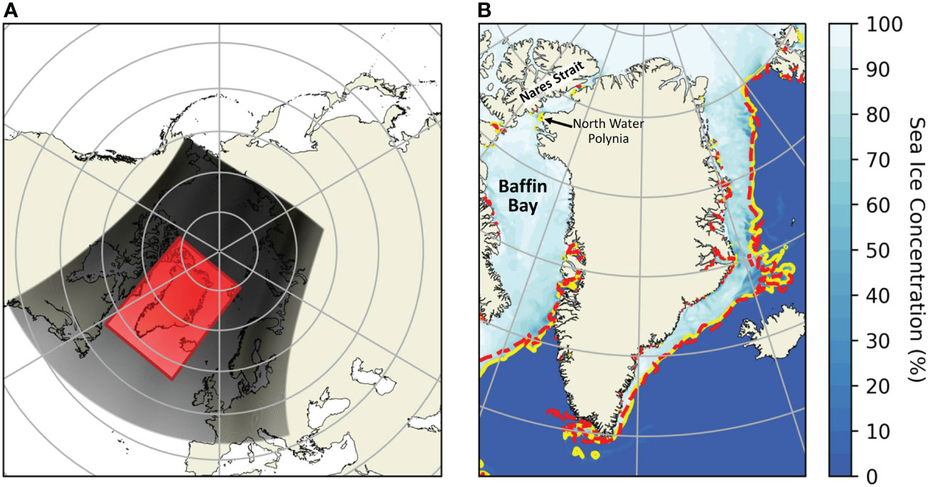
Figure 1 (A) Study region. Black and red shaded area define the operational model domain and the Greenland region from which the grid points are used in this study, respectively. (B) Demonstration-case (27/Apr/2021) of sea ice concentration estimated by the model (experiment v9; see below). The ice edge defined by the 15%-sea ice concentration contour is represented by the yellow line after the analysis at T=0 hours. The dashed red line shows the sea ice edge for the same forecast on day 6 forecast (T=144 hours; 03/May/2021).
This study introduces and conducts an inter-comparison of this forecast system and the latest operational remotely sensed-based sea ice services that DMI provides. The focus is on the sea ice edge location around Greenland as this is the main focus area for DMI and, at the same time, it is an essential diagnostic for mariners.
The article is organized as follows. Section 2 describes the materials and methods by introducing the high-resolution operational forecast system (Section 2.1), the re-analyses and the re-forecast experiments (Section 2.2), the atmospheric forcing (Section 2.3), the observational references (Section 2.4) used for evaluation purposes, and the verification metric (Section 2.5). The results related to the models’ evaluation in terms of sea ice concentration (Section 3.1), edge location (Section 3.2), and persistence (Section 3.3) are described and discussed in Section 3. Section 4 summarizes the main aspects of this work.
The newly-launched DMI sea ice operational forecast system (DMI-HYCOM-CICE) is based on the coupling of the 3D ocean model Hybrid Coordinate Ocean Model [HYCOM; Chassignet et al. (2007)] with the Community Ice CodE model [CICE; Hunke et al. (2021)] through the Earth System Modeling Framework [ESMF; DeLuca et al. (2012)]. The system predicts the ocean and sea ice states. Compared to its previous version (Madsen et al., 2016), the model set-up has been updated on many fronts. It now adopts a finer nominal horizontal resolution of 5 km in the northern regions and includes new parameterized features. The sea ice component is improved with parameterizations of land fast sea ice (Lemieux et al., 2016b) and melt-ponds, as well as enhanced with prognostic sea ice salinity and improved thermodynamics schemes (Turner and Hunke, 2015).
Formation of sea ice occurs at the ocean freezing temperature, and ocean melts sea ice from below, when the ocean temperature exceeds the sea ice melting temperature, which is determined by the salt content of the lowest sea ice layer. The freshwater and ice discharge from Greenland are upgraded using a detailed dataset from the Geological Survey of Denmark and Greenland (Mankoff et al., 2019; Mankoff et al., 2020a; Mankoff et al., 2020b). We calculated monthly means for each of the ∼ 50000 river-runoff outlets (29576 streams and 18902 “glacier margins”, ie. glacier meltwater) and distribute these to the nearest coastal grid cell. Similar to this, ice calving from 267 glaciers (solid ice discharge) is transformed into equivalent freshwater fluxes, implying that the ice immediately melts at the nearest ocean grid cell. In reality, the solid ice (icebergs and growlers) will melt underway and gradually decrease the surface salinity and temperature within the fjords and offshore for the part that survives. The solid ice discharge used is on average 55%±32% of the total discharge for the 267 glaciers, but this number is an overestimation, as it also includes submarine melting at the glacier termini and melting between the termini and the gate upstream the glacier (Enderlin et al., 2014; Mankoff et al., 2020b). When compared to the previous version, the total freshwater discharge from Greenland is increased by a factor of 15, resulting in decreased near-shore salinity and increased baroclinicity. This is expected to contribute to improve the coastal ocean currents and, consequently, the sea ice transport nearshore Greenland.
The DMI-HYCOM-CICE set-up covers the Arctic and the Atlantic Ocean north of 15°S for the ocean, whereas the sea ice model only covers a northern fraction of the entire grid making the system more computationally efficient and less I/O demanding (Figure 1; black shaded area). It is forced by weather forecasts provided by the European Centre for Medium-Range Weather Forecasts (ECMWF) according to the performed experiment. To constrain model errors related to the sea ice, DMI-HYCOM-CICE assimilates satellite-based sea ice concentration provided at near real-time by the Ocean and Sea Ice Satellite Application Facility (OSI SAF), product OSI-401-b (OSI SAF, 2017). Similarly, DMI-HYCOM CICE assimilates satellite-based sea surface temperatures provided by the Group for High Resolution Sea Surface Temperature [GHRSST, https://podaac.jpl.nasa.gov/GHRSST, Høyer et al. (2012); Høyer et al. (2014)]. The assimilation system is a nudging system which is described in Rasmussen et al. (2018).
To evaluate the performance of the model system three experiments were performed. They generated one re-analysis (v7) and two re-forecasts (v8 and v9). For details the reader is referred to Table 1 and Figure 2.
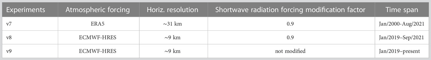
Table 1 Description of the three experiments (v7, v8, and v9), their atmospheric forcing and its modifications performed for the development of the DMI-HYCOM-CICE operational system.
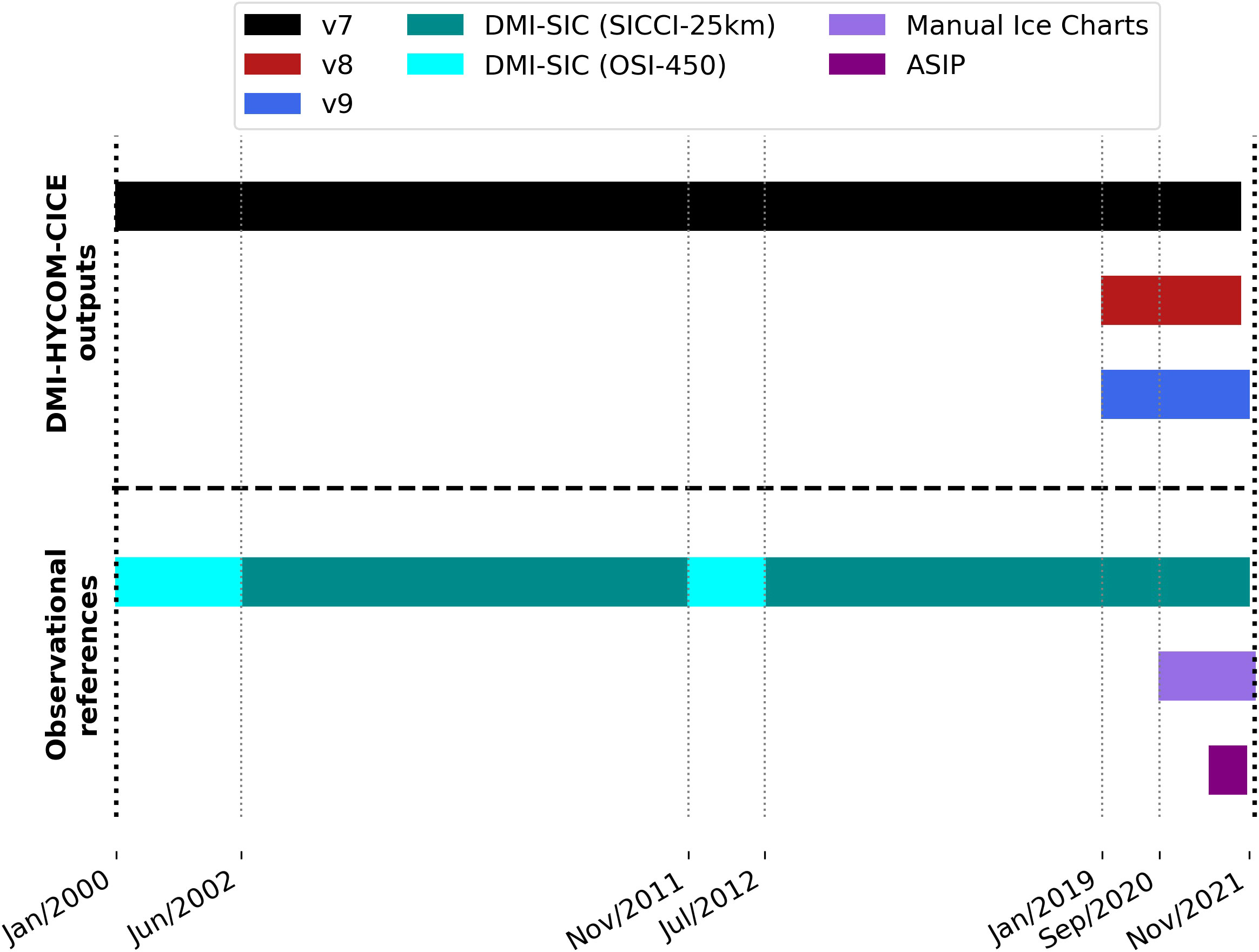
Figure 2 Data overview. Horizontal bars indicate the period covered by the DMI-HYCOM-CICE outputs (experiments v7, v8, and v9) and observational references (DMI-SIC, Manual Ice Charts, and Automated sea ice products (ASIP)). The period in which the DMI-SIC product derives from the SICCI-25km or OSI-450 product is also highlighted.
v7 is a re-analysis that assimilates sea surface temperature and sea ice concentration. The outputs from this simulation are comparable to the initial conditions of a forecast. This experiment spans Jan/2000-Aug/2021. v8 and v9 are re-forecasts that also assimilate sea surface temperatures and sea ice concentration from T=-24 to T=0, where T is hours from the initial conditions or the analysis. The v9 simulation continues from T=0 to T=144 (Figure 3). From T=0 to T=144 the re-forecast is comparable to the operational forecast run, except that the 144h atmospheric forecast consists of piece-wise 0-12h forecast slots rather than a full forecast from 0 to 144h. v8 spans Jan/2019-Sep/2021 and has been run for verification purposes. v9 also starts in Jan/2019 and keeps running to the present day as the operational version (Figure 2).
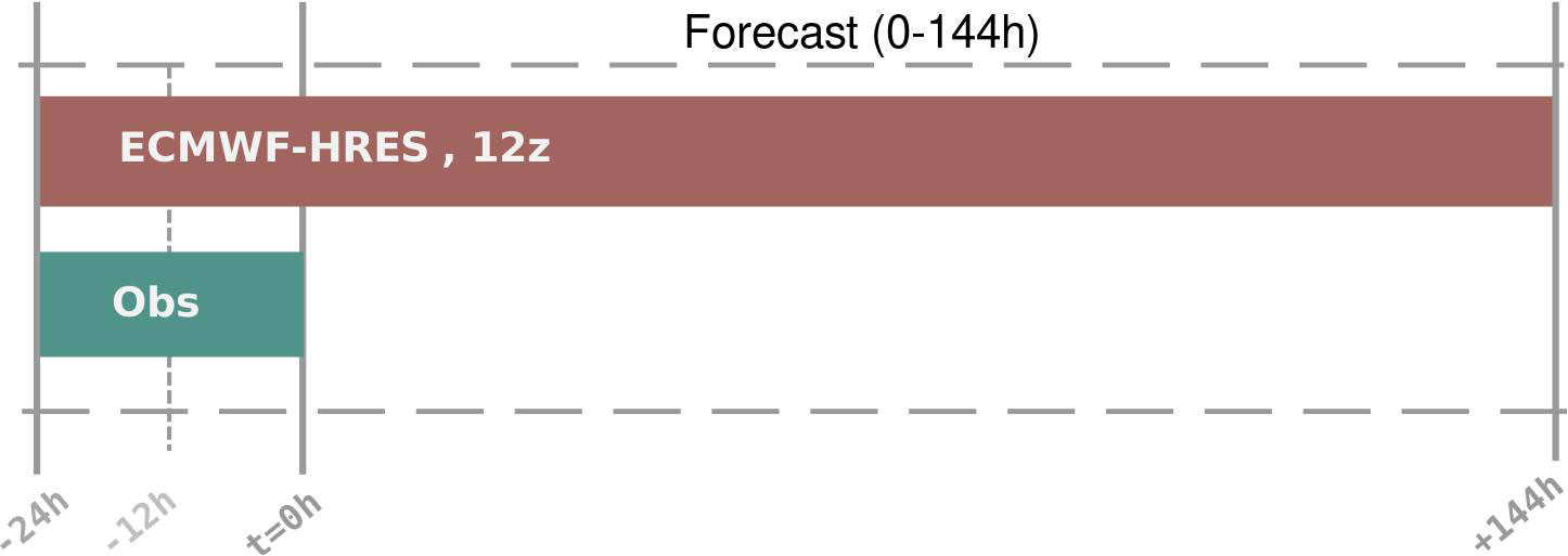
Figure 3 Overview of a forecast run. The brown bar indicates an 144 hours forecast that is initialized by 24h window when available observations (green bars) are assimilated. New forecasts are initiated with intervals of 12 hours and they are initiated from a restart file from the previous forecast.
As the final product, a 144 hourly forecast of sea ice conditions is produced twice a day and released on the Polar Portal (http://polarportal.dk/en/home/) and DMI ocean web-page (http://ocean.dmi.dk/) following the forecast schedule shown in Figure 3.
Two different atmospheric products from ECMWF have been used for the three experiments described in Section 2.2 (Table 1). The first experiment (v7) is forced by ERA5 (Hersbach et al., 2020) re-analysis with a horizontal resolution of ∼ 31 km. The second and third experiments (v8 and v9) are forced by ECMWF High-Resolution forecasts with ∼ 9 km resolution (ECMWF-HRES cy47r3; https://www.ecmwf.int/en/publications/ifs-documentation).
The ERA5 atmospheric forcing is examined by Hudson et al. (2019) over the Arctic region. These authors found that the cloud cover is underestimated during spring, which leads to an overestimation of the short-wave radiation and (less pronounced) underestimation of the downward long-wave radiation. As a result of this, ERA5 has a positive bias in the total downward radiation in spring. Similarly, they found the downward heat flux during summer was too high. One of the main issues in the boundary conditions is the lack of snow in re-analysis such as ERA5 (Arduini et al., 2022). An earlier study by Rasmussen et al. (2018) used the ice surface temperature bias between remotely sensed ice surface temperatures and a coupled ocean and sea ice model in order to correct the 2 m temperature and, based on this, the near-surface forcing. A more advanced approach by Zampieri et al. (2022) uses level 2 remotely sensed surface temperature data and a machine learning approach in order to correct the biases of the atmospheric re-analysis.
In order to acknowledge the challenges of the atmospheric re-analysis, a series of experiments with atmospheric surface corrections was carried out and the ice coverage was compared on the Arctic scale. The most suitable and simple correction was to reduce the downward short-wave radiation over sea ice by 10% as reproduced in experiment v7. By doing so, we reduce the total downward heat flux to the sea ice during the season with incoming solar radiation, which in turn provides a direct heat flux reduction in Watts per square meter. This mimics the net effect of adding Arctic cloud cover during spring and summer. The same correction was added to the v8 experiment, whereas experiment v9 uses the ECMWF-HRES atmospheric forcing. Table 2 lists the atmospheric forcing parameters and their GRIB field numbers for ERA5 and ECMWF-HRES. The specific humidity is calculated from pressure and dew temperature using the Arden Buck equation.
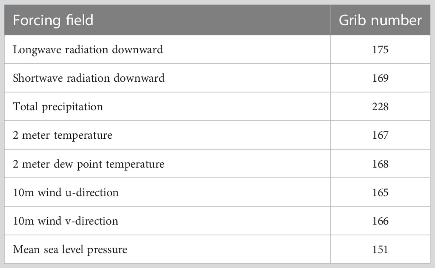
Table 2 Forcing fields from ERA5 and ECMWF-HRES.
Traditionally, a short-term sea-ice forecast has been run as the DMI-HYCOM-CICE, where a coupled ocean-sea ice model has been forced by an atmospheric reanalysis (e.g. Sakov et al., 2012; Madsen et al., 2016; Lellouche et al., 2018; Smith et al., 2021). Sea ice concentration is seen as an initial value problem that evolves slowly and an evolving sea ice cover has therefore not been included until recently in the atmospheric short-term forecast. Most studies that investigate an evolving sea ice cover within a short-term forecast focus on the weather. However, some studies point towards issues within the ocean and sea ice properties as well. Pellerin et al. (2004) show that a fully coupled system is better at forecasting fast coastal processes such as the formation of polynyas. Day et al. (2022) describe how the forcing may create large fluxes in a forced ocean-sea ice model due to a misplaced ice edge. This will force the modelled ice edge to converge towards the sea ice inherited within the atmospheric forcing.
For this experiment, ERA5, ECMWF-HRES and DMI-HYCOM-CICE are all controlled by the OSI SAF data set either as a surface boundary condition (ERA5) or through assimilation (ECMWF-HRES and DMI-HYCOM-CICE). This should ensure that the location of the ice edge is rather similar to the initial condition of the forecast.
Three state-of-the-art, satellite-based observational references are used in this work, as follows: (i) a newly-developed DMI sea ice concentration product (DMI-SIC); (ii) Manual Ice Charts produced at DMI, and (iii) automated sea ice product (ASIP) based on deep learning techniques also developed at DMI. Both (ii) and (iii) are distributed in the Copernicus Marine Service.
(i) The DMI-SIC product is a new release in which different sources of sea ice information have been combined and re-sampled onto a 0.05 ∘ regular latitude-longitude grid (Nielsen-Englyst et al., 2023). It is based on the EUMETSAT OSI SAF Global sea ice concentration CDR v2 product OSI-450 (covering 1979-2015) and the European Space Agency (ESA) Sea Ice Climate Change Initiative (SICCI) SICCI-25km sea ice concentration product (covering the following two periods: June 2002-October 2011 and July 2012-May 2017). An extension of the SICCI-25km processing was used to provide consistent sea ice concentration from May 2017 to May 2021 (hereafter referred to as SICCI-25km as well). The combined DMI-SIC product uses SICCI-25km whenever it is available and OSI-450 otherwise. Different filtering methods are used to improve the accuracy and consistency of the combined DMI-SIC product (Nielsen-Englyst et al., 2023).
(ii) The operational ice service at DMI produces ice charts based on manual interpretation of the satellite imagery, primarily from Synthetic Aperture Radar (SAR) sensors onboard the Copernicus Sentinel-1, but also other platforms such as Radarsat-2, the Radarsat Constellation Mission, TerraSAR-X and CosmoSkyMed. Optical and thermal infrared imagery from sensors onboard, e.g. Sentinel-2 and -3, are also used in the production when daylight and cloud cover is favorable. The ice charts are drawn within an ArcGIS production system with shape files as output. The ice charts map the ice concentration in polygons in 10s of % from 0-100% as defined by the World Meteorological Organization (WMO). The DMI ice charts do not have associated uncertainty estimates describing the ice concentration accuracy. However, a study of the differences between ice charts from the DMI ice service and the Norwegian ice service covering the same region shows a relatively large (up to 30%) standard deviation of the difference in ice concentration, especially at intermediate concentrations (20-80%), see Eastwood et al. (2022) (Appendix on ice chart uncertainty). The DMI ice charts are redistributed in the Copernicus Marine Service as gridded products resampled to 1 km × 1 km grid as the “Arctic Ocean - Sea Ice Concentration Charts - Svalbard and Greenland” (Dinessen et al., 2020), from which we use the “DMI overview ice chart” sub-product. The Overview ice charts are available through Copernicus Marine Service since September 2nd, 2020. The ice charts are produced twice weekly based on satellite data that is up to three days old, which is the time needed in order to cover our region of interest - Greenlandic waters.
(iii) The ASIP (Automated Sea Ice Products) sea ice concentration data set is produced by DMI using the ASIP deep learning algorithm, which is a further development of Malmgren-Hansen et al. (2021). The ASIP sea ice concentration products are automatically retrieved from Copernicus Sentinel-1 Synthetic Aperture Radar (SAR) satellite imagery (in Extra Wide (EW) and Interferometric Wide (IW) swath mode, both re-sampled to an 80 m grid, being close to the native spatial resolution in EW mode) by using a Convolutional Neural Network (CNN) that fuses the high-resolution SAR images with coarser resolution passive microwave observations from the AMSR2 sensor onboard JAXA’s GCOM-W satellite in order to produce detailed maps of the sea ice conditions. The CNN is trained on DMI ice charts that are contained in the AI4Arctic/ASIP Sea Ice Dataset v2 (Saldo et al., 2021). This means that any bias introduced by the manual ice charting method (e.g. an overestimation of intermediate SICs) is inherent in the ASIP model. However, any inter- and intra-ice analyst variability are not reproduced by the ASIP algorithm. ASIP algorithm outputs sea ice products distributed within the Copernicus Marine Service as the “DMI-ASIP sea ice classification - Greenland” (Dinessen et al., 2022). For this study, 14-day mosaics were created from individual ASIP products, with the newest ASIP product on top”, and with the mosaics’ end-date corresponding to the datestamp of the DMI Overview ice charts. Although the ASIP mosaics are composed of up to 14 days of data, in practice, almost the entire Greenland waters are covered by data within 3 days.
It is worthwhile to mention that the observational references (DMI-SIC and the Manual Ice Charts) used for validation purposes are different from the data assimilated by the model (OSI-401-b) and also from themselves. Except for two relatively short periods when OSI-450 is merged into the DMI-SIC product (Jan/2000–Jun/2002 and Nov/2011–Jul/2012). These two periods do not overlap the v8 and v9 experiments. Figure 2 presents an overview of the model and observational data sets used in this work regarding their time coverage.
Observational products are interpolated onto the HYCOM-CICE grid to make the data from different sources straightforwardly comparable. We apply the Integrated Ice Edge Error [IIEE; Goessling et al. (2016)] as verification metric for evaluating the ability of the model in predicting the sea ice edge provided by the observational references, as well as to compare the observational references themselves. Hereafter, we adopt the definition in which the sea ice edge location is determined by the 15%-sea ice concentration threshold (note that this differs from the WMO Sea Ice Nomenclature definition of sea ice edge – 0%). The IIEE quantifies the total area where the predicted sea ice disagrees on the sea ice concentration being above or below 15%. Therefore, the IIEE is given by the sum of the areas from all grid cells where the modeled sea ice (or the second observational reference) overestimates (O) or underestimates (U) the “true” reference regarding the 15% threshold so that IIEE = O+U.
Figure 4 provides examples of the IIEE metric applied to our data sets for four different days (columns), one from each season. Comparisons are made between HYCOM-CICE (v9) vs. DMI-SIC, HYCOM-CICE (v9) vs. Manual Ice Charts, and DMI-SIC vs. Manual Ice Charts. As an assumption, we consider the later product from each pair of comparisons as the “true” reference. Therefore, red colors in Figure 4 indicate that the first product overestimates the sea ice edge of the reference product, while blue colors reveal the opposite.
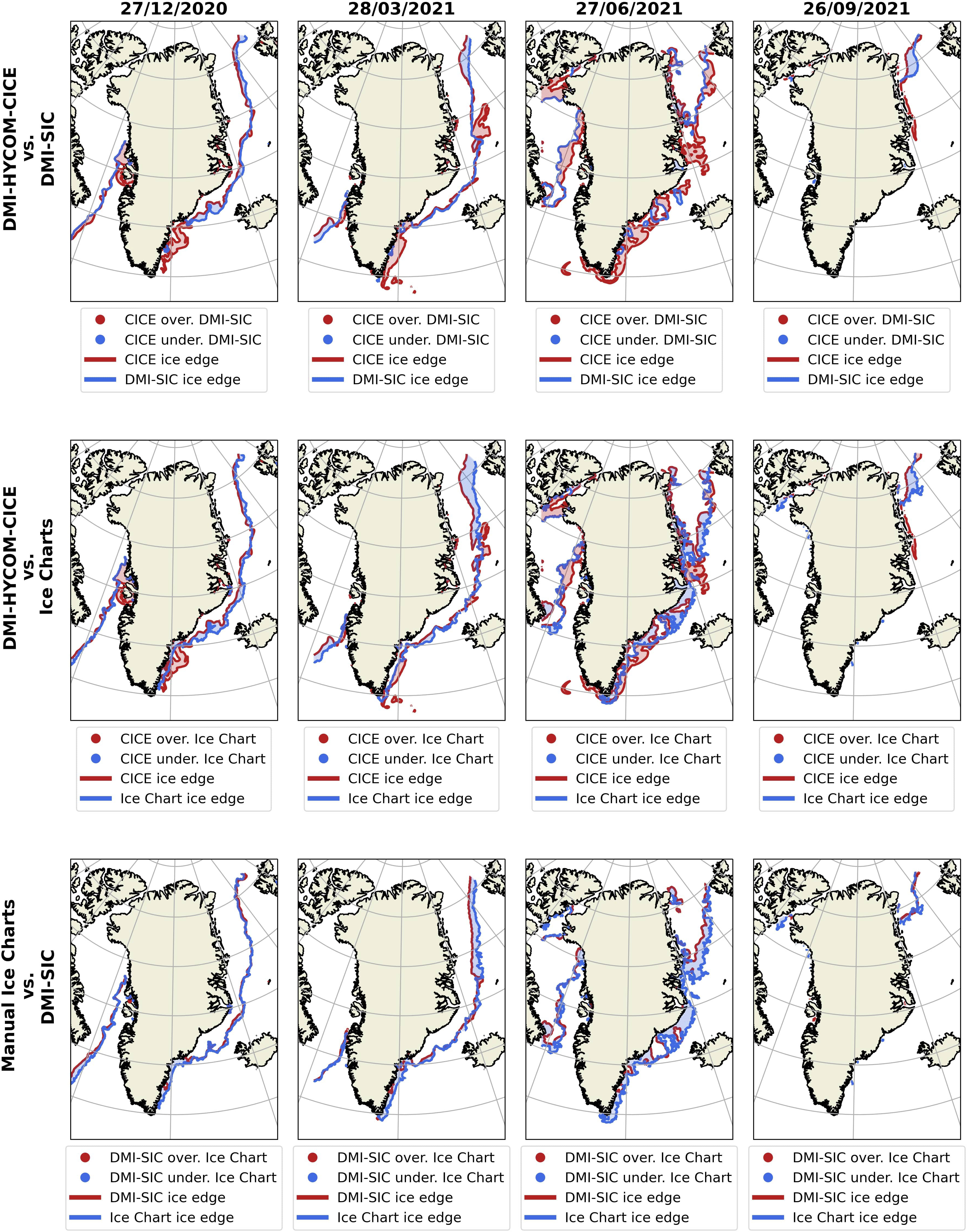
Figure 4 Snapshots of IIEE (see definition in section 2.5). Each column represents one day as displayed in the header. Top row: IIEE maps of DMI-HYCOM-CICE (V9) vs. DMI-SIC. Red and blue indicate whether DMI-HYCOM-CICE overestimates or underestimates the ice edge prescribed by DMI-SIC, respectively. Middle row: Same as top row but IIEE maps of DMI-HYCOM-CICE vs. Manual Ice Charts. Bottom row: Same as top row but it compares DMI-SIC vs. Manual Ice Charts (same order).
Section 3.1 and Section 3.2 both focus on validation of the initial conditions, whereas Section 3.3 addresses the evaluation of the forecast skill.
The sea ice edge is defined by the sea ice concentration field, therefore we will start by providing a first assessment of the DMI-HYCOM-CICE sea ice concentration outputs. We promote an averaged-based, month-by-month comparison of our v7 experiment against the DMI-SIC observational product. This comparison covers the period from Jan/2000 to Dec/2020, which represents the entire overlapping period of the two products (see Figure 2). Figure 5 shows that, on average, there is a good agreement between DMI-HYCOM-CICE and the observational reference. Overall, the model slightly underestimates the observations in almost all months outside of the melt season, as indicated by light shades of blue (differences smaller than 10%). Notice that from October to April, when sea ice is growing, the model underestimates the sea ice concentration near the sea ice edge in both the western and eastern Greenlandic coast.
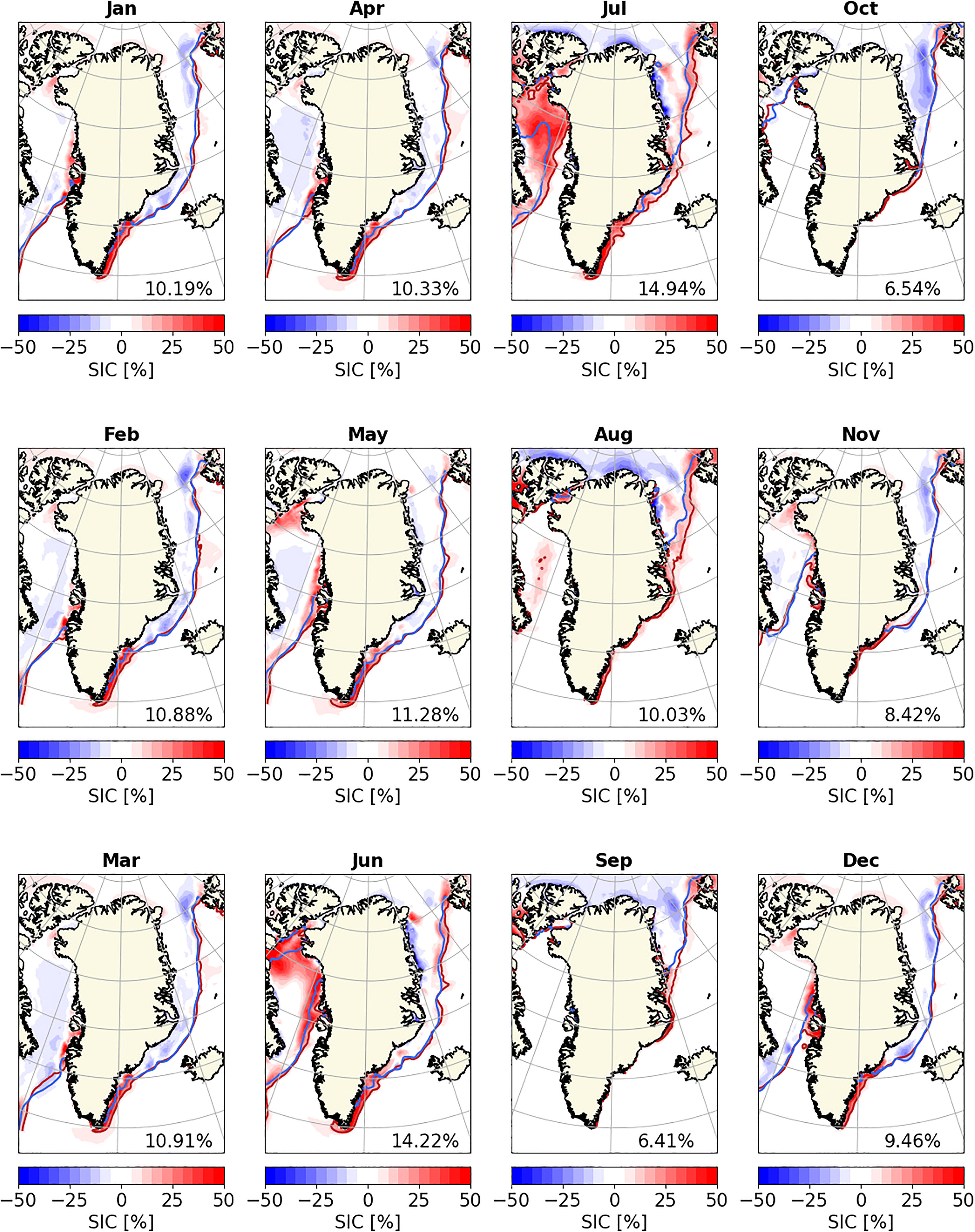
Figure 5 Mean difference (v7 - DMI-SIC) in sea ice concentration (%) estimated for each month (from Jan/2000 to Dec/2020) between the v7 experiment and the DMI-SIC reference product. Blue and red lines display the mean sea ice edge represented by the 15% sea ice concentration contour for the DMI-SIC and v7 outputs, respectively. The percentages given in the bottom right are the area-weighted root mean squared errors for the respective panels.
On the other hand, the model overestimates the sea ice concentration near the southeastern Greenlandic coast whenever the region is sea ice covered, from December to July. The reason for this incongruence is in part linked to limitations of the observational reference itself, as discussed in section 3.2.3. DMI-HYCOM-CICE also overestimates the sea ice concentration in the Baffin Bay when the sea ice starts to melt around May with the opening of the North Water Polynya in the northern extremity of the bay, between Greenland and Canada, and also adjacent to the western Greenlandic coast. The bias in the northern part of Baffin Bay is likely due to the sea ice model dynamics and the challenge of forming the ice bridge in the southern part of Nares Strait (e.g., Rasmussen et al., 2010; Dansereau et al., 2017; Plante et al., 2020). The approach by Shlyaeva et al. (2016) improved the challenges of modeling landfast sea ice by creating an ensemble member without sea ice dynamics. However, it does not improve the sea ice physics and it will cause problems if the ice bridge collapses during a forecast. The positive bias between model and observations grows throughout the melt season, but it vanishes in August and September when sea ice is entirely melted in that region including in the model outputs. Likewise, the model overestimates the sea ice concentration along the eastern sea ice edge around the same period.
The fact that the model underestimates the sea ice concentration from approximately October to April, and overestimates it during the melting season in the Baffin Bay and along the eastern Greenlandic coast, suggests that DMI-HYCOM-CICE is a few days delayed with the seawater freezing-up and sea ice breaking-/melting-up compared to the observations. Nevertheless, the relatively higher differences in June and July may partly be linked to higher uncertainties of the DMI-SIC product during these months, characterized by substantial melt-ponds coverage, as discussed in Section 3.2.3.
To provide a measure of the monthly differences shown in Figure 5, we calculated the area-weighted root mean squared errors (AW-RMSEs) for the monthly maps. The last four months of the year present smaller AW-RMSEs: 6.4% (September), 6.5% (October), 8.4% (November), and 9.5% (December). AW-RMSEs are similar from January to April, and August, ranging from 10.0% to 10.9%. Maximum AW-RMSEs take place in May (11.3%), June (14.2%), and July (14.9%), which is mainly due to the melting-season biases in the Baffin Bay discussed above.
Figure 6A illustrates how the IIEE evolves from 01/Jan/2000 to 30/Sep/2021 when comparing the v7 experiment and the DMI-SIC product. In the long-term, the IIEE is stable and it does not present significant trends (Figure 6A, black line). From the mean IIEE = 2.61 (± 1.23) × 105 km2 , the largest part of the standard deviation is the seasonal cycle rather than interannual variations or estimations of the mean. About 74% of the mean IIEE are due to the overestimation (Figure 6A, red line) of the sea ice edge by the model (O = 1.93(± 1.18)× 105 km2 ), while the remaining 26% are due to an underestimation (blue line; U = 0.68(± 0.35)× 105 km2 ).
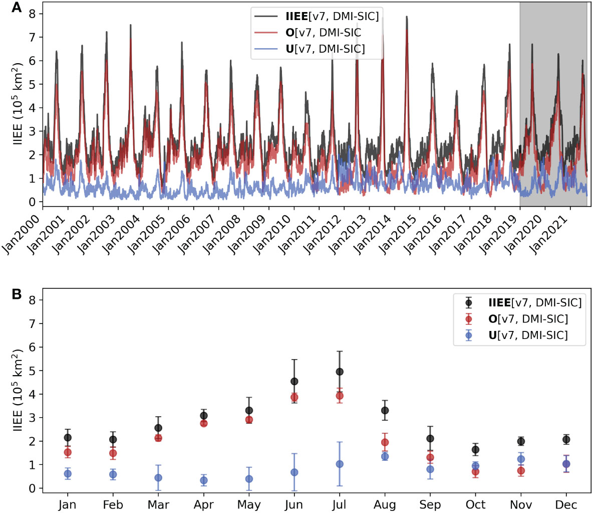
Figure 6 (A) Integrated Ice Edge Error (IIEE) estimated between the v7 experiment and DMI-SIC (black line), and its corresponding overestimated (red line) and underestimated (blue line) components. (B) Average monthly IIEE calculated for the time series displayed in (A), calculated for the period Jan/2000–Dec/2020. Vertical bars indicate the 1-standard deviation interval.
The IIEE has a marked seasonal variation with values that grow throughout the melt season and peak in July when IIEE = 4.95(± 0.86)× 105 km2 (Figure 6B). In the period from Sep–Mar, the IIEE is smaller than 2.60 × 10⁵ km2 . The IIEE growth in the melt season is mainly linked to the errors associated with an overestimation of the sea ice edge by the model (Figures 6A, B).
Even though the IIEE does not present a trend for the entire time span, and the higher errors in the warmer season are always explained by overestimation, the long-term time series shows two distinguished behaviours in the melt season. From Jan/2000 to Dec/2010, average values calculated from Sep-Mar indicate that errors due to overestimation (O = 1.56(± 0.60)× 105 km2 ) are higher than the underestimation (U = 0.47(± 0.23)× 105 km2 ) contribution. Nevertheless, from Jan/2011 to Dec/2018, the contributions to the IIEE are more equally distributed between overestimation (O = 0.99(± 0.39)× 105 km5) and underestimation (U = 0.89(± 0.35)× 105 km5) cases. We do not have a clear understanding for that behaviour.
As indicated by the mean sea ice edge contour for the individual months in Figure 7 (red and blue lines), there is a striking correspondence between model and observations throughout the year in terms of monthly averages. Figure 7 also displays the cumulative occurrence of days (in percentage) that v7 outputs disagree from the observations by overestimating or underestimating the sea ice edge. Again, the main differences are observed in the warmer seasons, mainly in June and July, in the northern Baffin Bay. Some mismatches also take place during summer off eastern Greenlandic coast, when the modeled ice edge is further offshore than the observed sea ice edge. Nevertheless, the maximum percentage of days in which mismatches take place in the eastern ice edge does not exceed 30–40% in August. Such a difference is even smaller in June, July, and September.
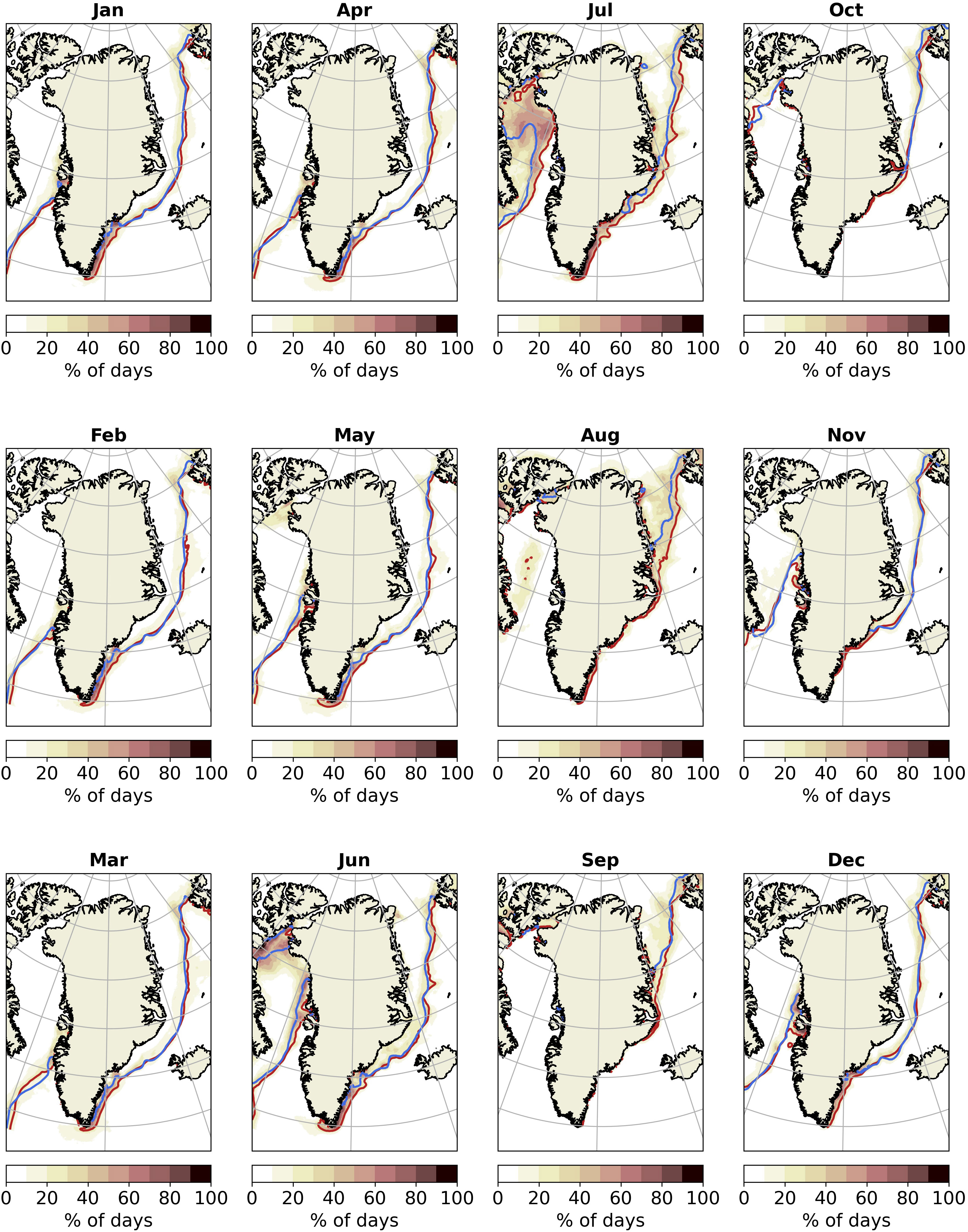
Figure 7 Cumulative occurrence of days (in percentage) in which the model outputs from v7 experiment overestimates or underestimates the DMI-SIC observational product based on the IIEE metric. The calculation spans for 21 years (Jan/2000-Dec/2020). Blue and red lines display the mean sea ice edge represented by the 15% sea ice concentration contour for the DMI-SIC and v7 outputs, respectively.
To refine the model set-up for the operational forecast system, three different experiments are investigated using coarse resolution ERA5 atmospheric reanalysis with modified short wave radiation (v7), and similar using high resolution ECMWF-HRES forcing with (v8) and without (v9) short wave modifications as detailed in Section 2.3. The experiments overlap for almost 3 years from Jan/2019 to late 2021 (see Figure 2).
By comparing experiment v7 against v8, Figure 8A reveals that the two ECMWF forcings do not have a noticeable influence on the integrated errors associated with the forecast of the sea ice edge despite their different resolution. Regarding the shortwave modifications, the non-negligible improvement (smaller IIEE values) for v9 compared to v8 in summer (mainly in July) indicates that a 10% reduction in this variable may be a too strong forcing modification. It corroborates that the ECMWF-HRES does not need forcing modifications in the DMI-HYCOM-CICE standard version, at least for this study region and setup (Figures 8A, B).
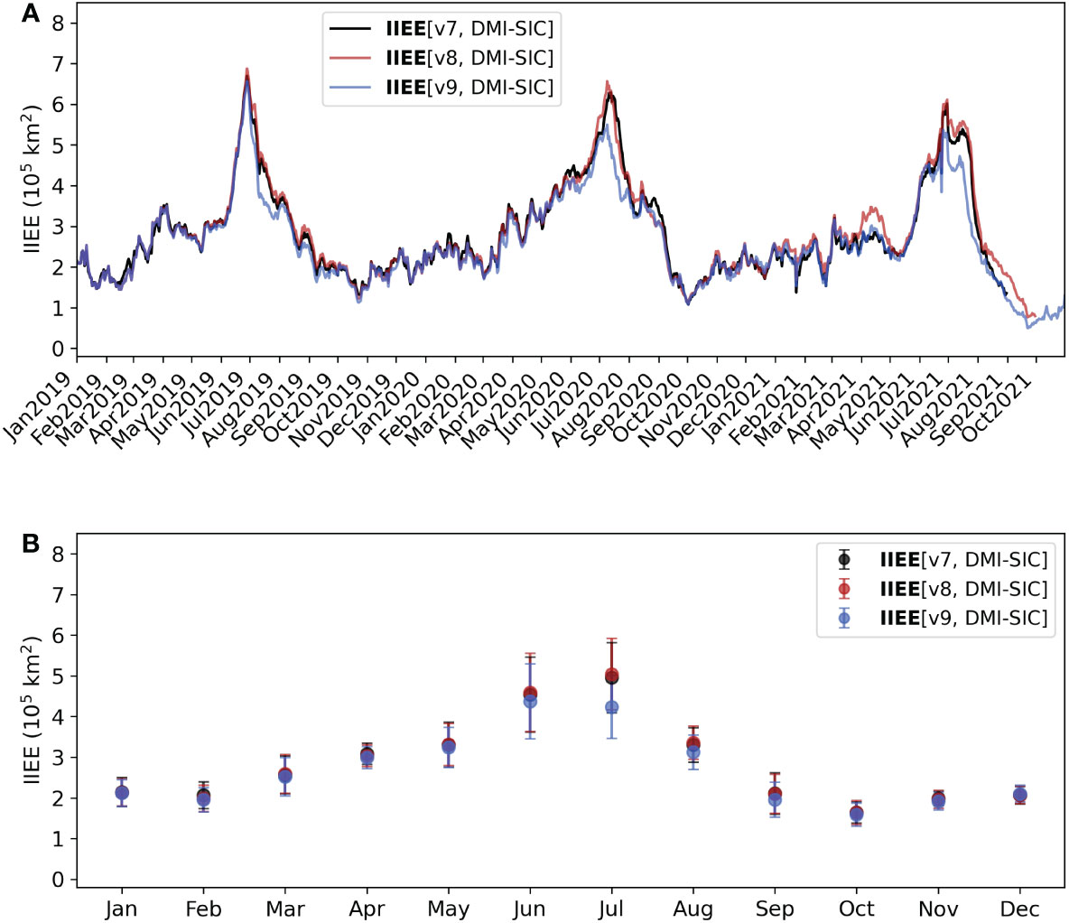
Figure 8 (A) Integrated Ice Edge Error (IIEE) estimated between the v7 (black line), v8 (red line), and v9 (blue line) experiments and DMI-SIC. (B) Average monthly IIEE calculated for the time series displayed in (A), calculated for the period Jan/2000–Dec/2020. Vertical bars indicate the 1-standard deviation interval.
By definition, the IIEE plotted over time in Figure 8 displays a diagnostic integrated for the entire study region. Therefore, this diagnostic does not specify the grid points where the model and observations agree, or not (over- or underestimate), in terms of sea ice edge location. Figure 9 overcomes this limitation by plotting the number of days (in percentage) in which the three experiments overestimate (first column) and underestimate (second column) the sea ice edge location provided by the observational reference. Figure 9’s third column shows the total occurrence of days in which the model and observations disagree in either way. The three experiments present a marked resemblance regarding the number of days and regions of discrepancy. Over time, there is a clear pattern of how the sea ice edge mismatches are distributed in space, although the two data sets barely disagree in more than 30% of the total number of days. DMI-HYCOM-CICE slightly overestimates the sea ice edge in the Baffin Bay and off southeastern Greenlandic coast (Figure 9; first column) and underestimates it off northeastern Greenlandic coast (Figure 9; second column).
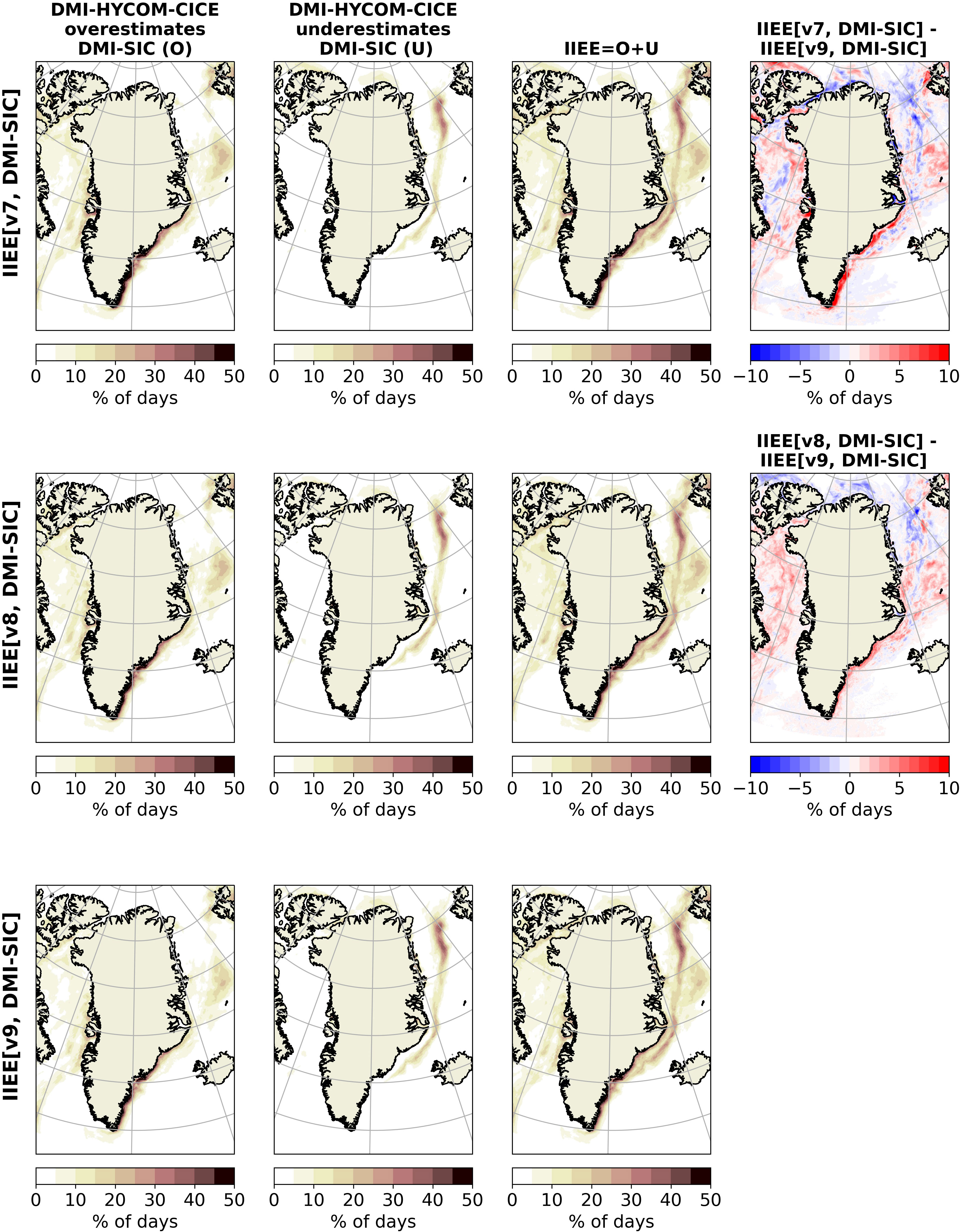
Figure 9 Cumulative occurrence of days (in percentage) in which the model outputs from v7 (first row), v8 (second row), and v9 (third row) experiments overestimate (first column) or underestimate (second column) the DMI-SIC observational product regarding the 15% sea ice concentration threshold. The third column shows both overestimation and underestimation cases. The fourth column shows the differences IIEE[v9, DMI-SIC] - IIEE[v7, DMI-SIC] (first row) and IIEE[v9, DMI-SIC] - IIEE[v8, DMI-SIC] (second row).
The spatial improvements highlighted by the dominance of shades of red in Figure 9’s fourth column, associated with the smaller errors in summer shown in Figure 8, indicates that adopting the v9 experimental configuration upgrades the forecast skill of the sea ice edge for almost the entire domain, except in the north of Greenland. The clearest improvement is adjacent to the southeastern coast. Due to these improvements, the v9 configuration with ECMWF-HRES forcing and no forcing modification is selected as the operational version of our forecast system for sea ice conditions off Greenland.
Despite having a certain degree of subjectivity and being restricted in time, with twice-weekly releases available at the Copernicus Marine Services from Sep/2020 (120 images in total for this study), Manual Ice Charts provide a valuable opportunity for promoting an additional and independent evaluation of our forecast system as they are often considered to be the best available product, especially in terms of the ice edge. In addition to this, the recently developed ASIP product is included in the comparison. Considering these products also allow an estimation of the observational uncertainty itself through comparisons against the DMI-SIC product.
Figure 10A indicates that IIEE values resulting from the evaluation of v9 experiments are very similar when adopting either DMI-SIC (red dots) or Manual Ice Charts (blue dots) as observational reference. Interestingly, the IIEEs calculated between both observational products follow the same temporal pattern with values peaking in summer. This fact reveals that larger values of IIEE in summer, as shown in Figures 6, 8, are not only related to the model but in part resulting from observational uncertainties (Figure 10A, black dots). By comparing ASIP and Manual Ice Charts (Figure 10A, magenta crosses), two similar observational products, IIEE values are further reduced mainly in the (warm) summer season. Nevertheless, these results should be interpreted with caution since the ASIP algorithm is trained on Manual Ice Charts and might reproduce any systematic biases found in the charts, as described in Section 2.4.
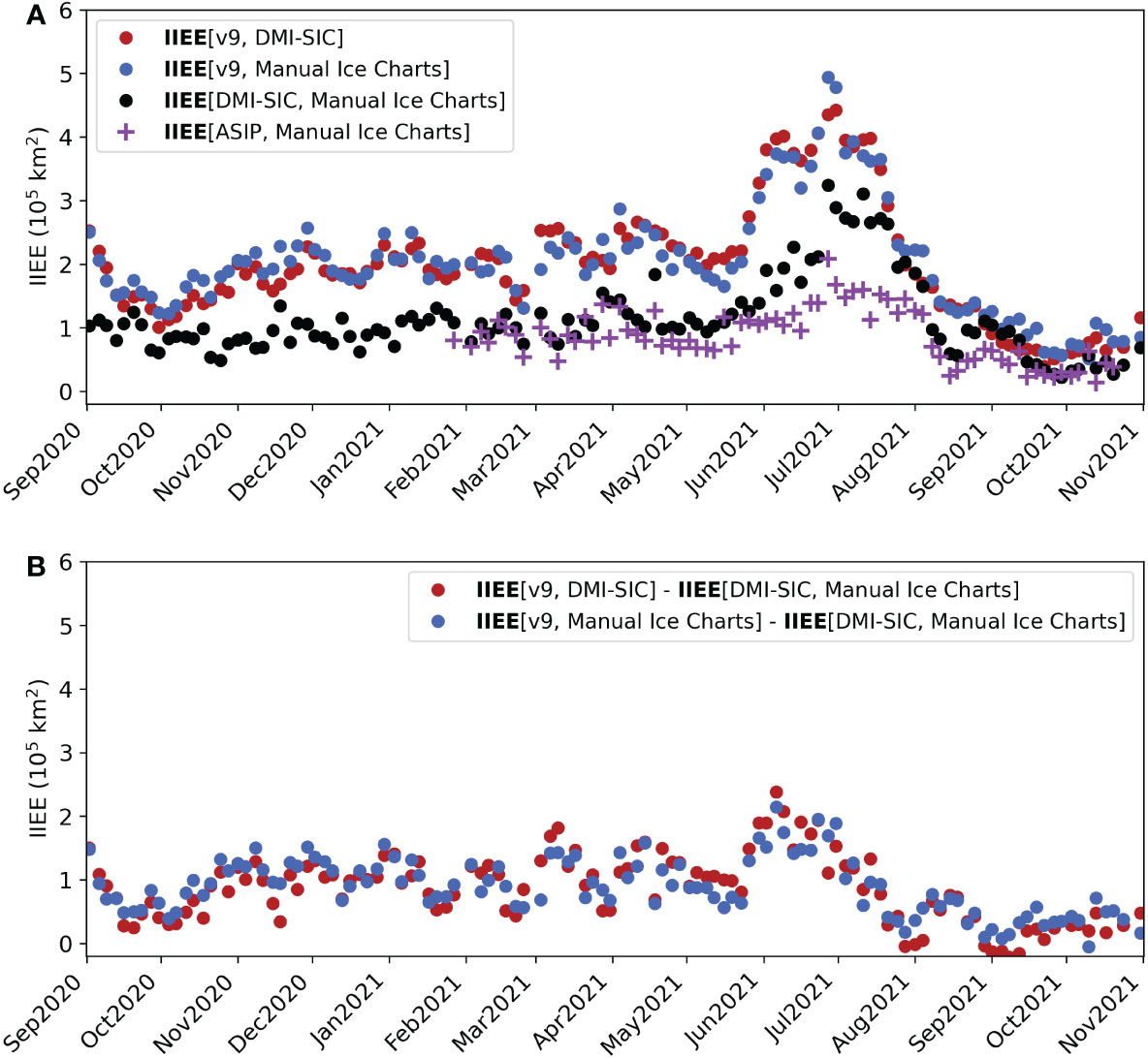
Figure 10 (A) Integrated Ice Edge Error (IIEE) estimated between the v9 experiment and the observational products: DMI-SIC (red dots) and Manual Ice Charts (blue dots). The black dots show the observational uncertainty given by the IIEE calculated between DMI-SIC and Manual Ice Charts and similar between ASIP and Manual Ice Charts given by the magenta plus markers. (B) Difference between the IIEE resulting from the comparison between model–observations and the observational uncertainty. The computation is performed only for dates in which Manual Ice Charts are available.
Figure 10B reveals, by subtracting the observational uncertainty (IIEE[DMI-SIC, Manual Ice Charts]), that the relative IIEE is more stable over time and reduces by about 41% and 44% for the v9–DMI-SIC and v9–Manual Ice Charts comparisons. This indicates that assimilation of the ASIP product might improve the initial state of the operational sea ice model around Greenland, especially in summertime, when the largest bias occurs.
Analogously to Figure 9, but now comparing v9 vs. DMI-SIC, v9 vs. Manual Ice Charts, and DMI-SIC vs. Manual Ice Charts, Figure 11 shows the percentage of days in which a pair of sea ice concentration data sets disagree regarding the 15%-SIC threshold. Figure 11’s first column shows that the IIEE due to the overestimation of the sea ice edge by the model (v9 experiment) is evident off the southeastern Greenlandic coast. This overestimation is higher when comparing v9 against DMI-SIC and attenuated when model outputs are compared against the Manual Ice Charts. Along the eastern and northeastern coast the errors are mainly associated with an underestimation of the sea ice edge by the model (Figure 11, second column). Reinforcing the results shown in Figure 10, the IIEE are smaller when comparing the observational products (Figure 11, fourth column). Also, the IIEE between the observational products are mainly due to an underestimation of the sea ice edge by the DMI-SIC product compared to the Manual Ice Charts (Figure 11, third row). DMI-SIC and other passive microwave products have issues near the coast where the satellite images are contaminated by land and provide erroneous results. In the southeastern part of Greenland the sea ice cover is a near-coastal narrow band, which limits the information from passive microwave data.
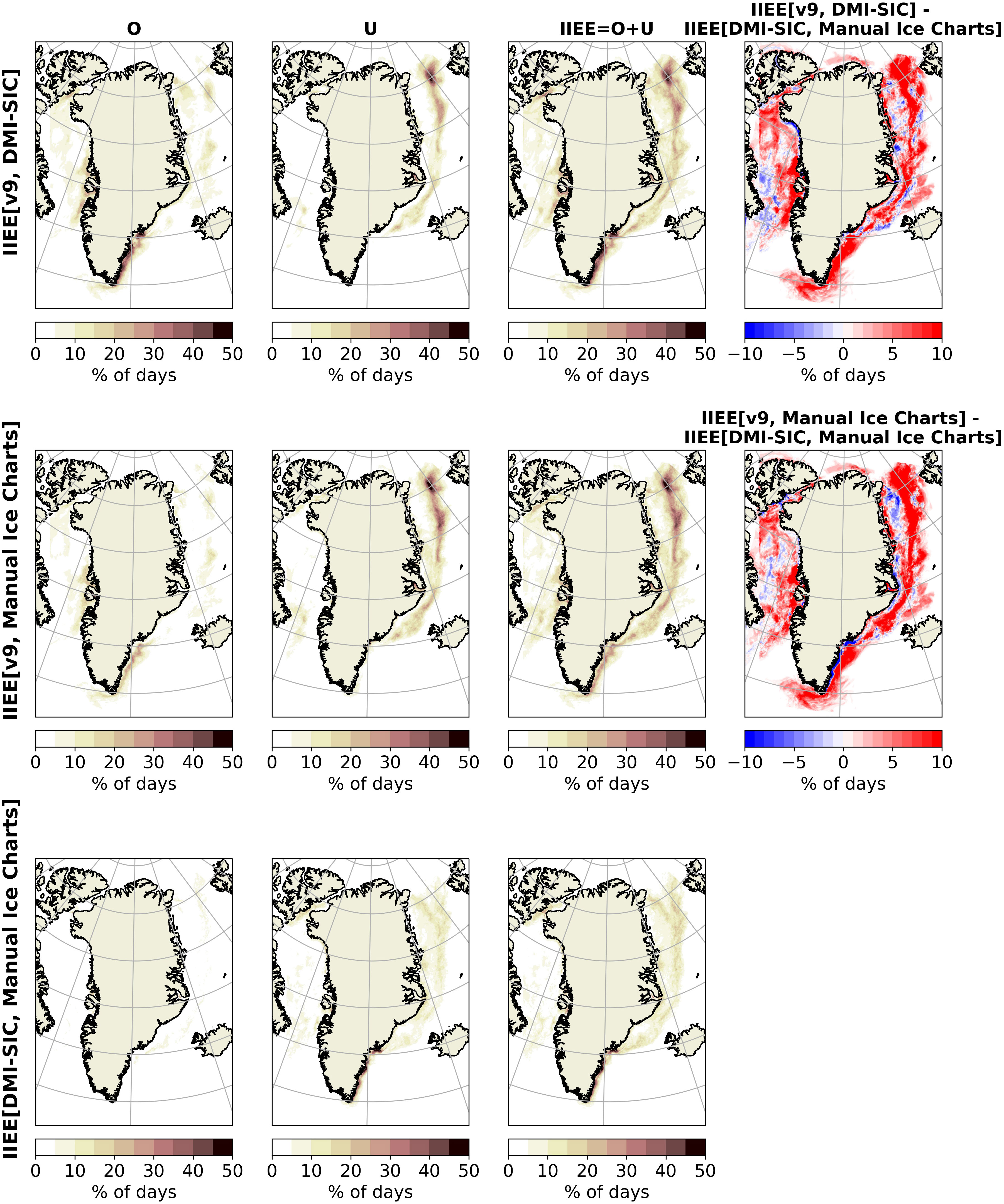
Figure 11 Same as Figure 9 but comparing the v9 experiments, and the DMI-SIC and Manual Ice Charts observational products.
To complement these results, the supplemental material of this manuscript brings an animation that displays the IIEE computation, partitioned in contributions due to overestimation and underestimation, between model outputs and observational products. It sequentially shows all 120 dates with available Manual Ice Charts. The animation makes it easier to visualize the results discussed throughout this manuscript. Nevertheless, it also allows us to identify other minor imperfections of the model. The most remarkable is the overestimation of the sea ice edge by the model in the southern tip of Greenland (e.g., 03/Feb/2021 and 07/Mar/2021). Given that these coastal seas have been marked out as the windiest location in the world ocean (Sampe and Xie, 2007), the likely explanation for this overestimation is related to the fact that the sea ice model does not account for the ocean waves and swells impinging the ice edge from offshore, and the system that provides the ECMWF-HRES forcing does not, either. These waves are recognized as an important agent for sea ice disintegration, mainly in the melt season (Squire et al., 1995; Squire, 2007; Li et al., 2021)
An example of the evolution of a forecast is seen in Figure 1B. The yellow contour shows the forecast at the initial condition, whereas the dashed red contour shows the forecast at T=144. For this case, it is clear that compared to the total ice cover the changes are limited, however north of Iceland and in the southwestern corner of the domain near the ice edge the yellow and red contours differ.
In order to quantify the skill of the operational forecast, the experiment v9 is evaluated against persistence as in Lemieux et al. (2016a) and following Equation 1:
where Pn and Fn denotes the IIEE calculated between observation (OBS) and forecast at day 0 (FC0) and day n (FCn), respectively. As observational reference, DMI-SIC is used, as it exists every day for the entire v9 period. If the solution for Equation 1 is positive, the forecast is better than persistence.
The temporal variation of the forecast skill against persistence is shown in Figure 12, and statistics are given in Table 3. The forecast is in general better than persistence. The improvement of the re-forecast skill compared to the persistence forecast increases by around 10% from the 1 day forecast (66%) to the 6 days forecast (76%). However, the initial IIEE is still the largest part of the bias, thus this should be a focus area in future developments. In summertime, when the biases are largest, the re-forecast skill towards persistence is also largest.
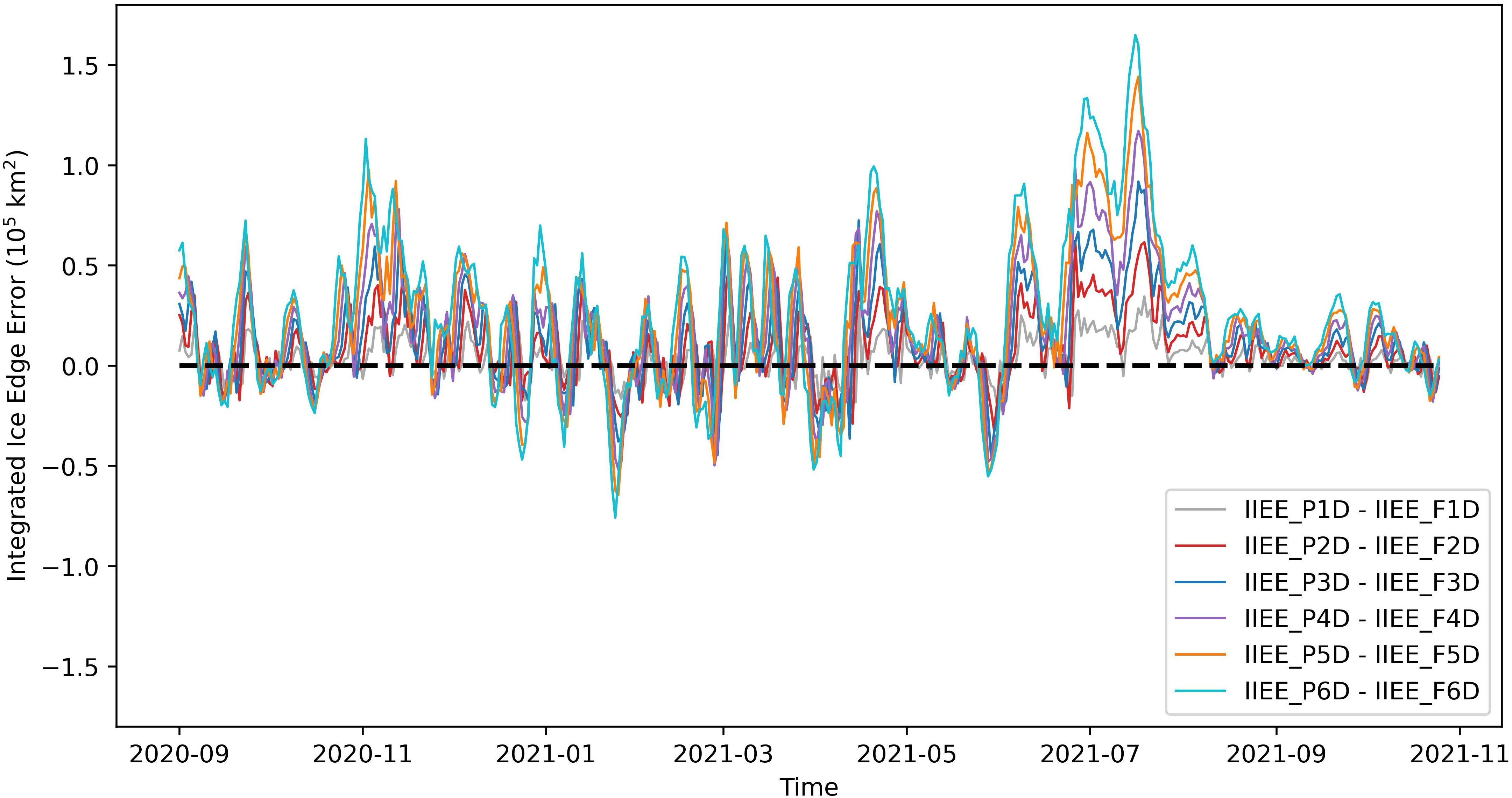
Figure 12 IIEE difference of persistence minus forecast for v9 experiment vs. DMI SIC product. The lines represent the result after 1 to 6 days.
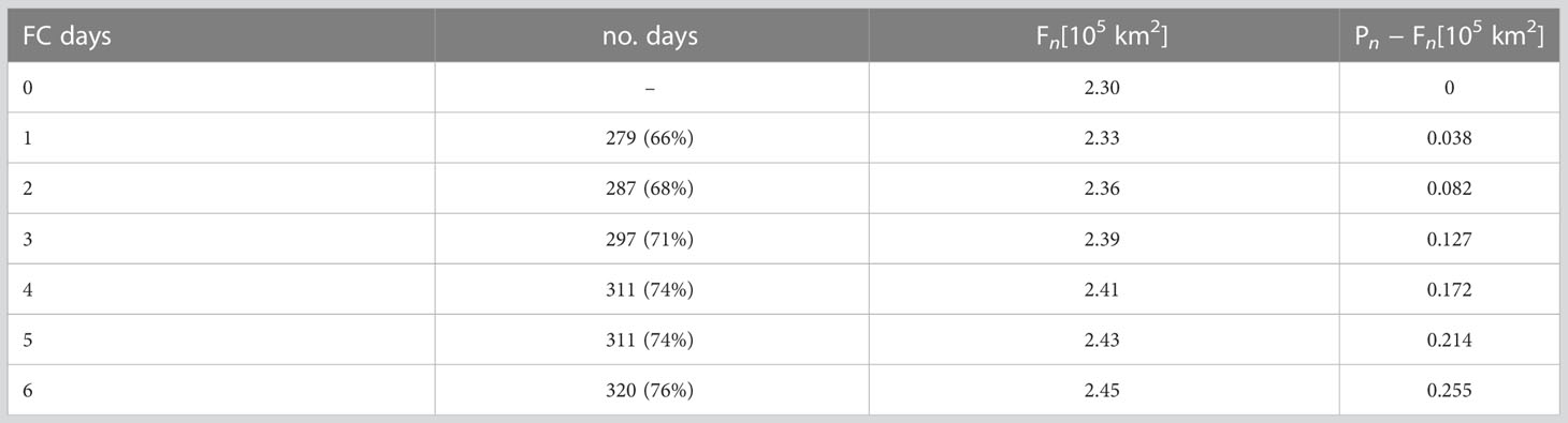
Table 3 Persistence vs. forecast. First column is the forecast day. Second column is the number of days where forecast is better than persistence (out of 420 days). Third column is the IEEE for forecast against DMI-SIC (Fn), and the last column is the IEEE differences between persistence (Pn) and forecast (Fn).
This article introduced the recently-launched, DMI operational forecast system for sea ice conditions off the Greenlandic coast. The system is built on the coupling of the ocean model HYCOM and the sea ice model CICE. These are, in turn, forced by ECMWF deterministic atmospheric forcing and assimilate near-real-time satellite observations of sea ice concentration from OSI SAF (OSI-401-b). The model set-up for the operational version is chosen based on the evaluation of three experiments. It provides 144-hourly forecasts of sea ice conditions twice a day, supporting mariners with voyage planning and safety at sea (see Secs. 2.1 and 2.3).
We here provided a first evaluation of the forecast system by inspecting its ability to predict the sea ice edge location. To do so, we calculated the integrated ice edge error metric (see Section 2.5) between the DMI-HYCOM-CICE outputs against three satellite-based observational references: DMI-SIC, Manual Ice Charts, and ASIP (see Section 2.4). Since these products are based on different methods to convert retrievals of satellite observations into sea ice properties, it also allowed us to provide an estimate of the observational uncertainty.
Altogether the model provides robust forecasts of the sea ice edge throughout the year, although improvements during late spring and summer are desirable (see Section 3). In May, the forecast system is delayed a few days in reproducing the opening of the North Water Polynya in northern Baffin Bay. At the same time, the model is also delayed in the retreat of sea ice off the western Greenlandic coast. This delay in the model persists during summer when sea ice is melting in the entire Baffin Bay (see Figures 5, 7). Due to that, the highest values in the integrated ice edge error are observed in late spring and summer. The delay of the sea ice retreat may be linked to the warm currents along the western coast of Greenland not being properly modeled (Buch, 2002). Likewise, it could also be linked to the usage of passive microwave-based products, that can have issues with melt ponds during summer by interpreting them as open water, which lead to ice concentrations that are biased low (see Figures 6, 8).
The forecast of the ice edge was tested against persistence. The forecast is better than persistence in 66% of the days when the forecast is made with one day lead time and 76% percent of the days when the forecast is provided with 6 days lead time. The skill of the forecast is especially pronounced during summer, when the model biases are highest.
Off the southeastern coast of Greenland, the model also overestimates the observations in summer by predicting a sea ice edge further offshore (see Figures 5, 7). A potential reason for explaining this delay during the melt season is the fact that the model does not account for the waves interacting with the sea ice edge. Waves are important for the sea ice disintegration, especially considering that this area is extremely windy (Sampe and Xie, 2007). Nevertheless, part of the integrated ice edge errors found off the eastern Greenlandic coast might also be associated with observational uncertainties. Our results show that two independent observational references (DMI-SIC and Manual Ice Charts) also disagree in this region, especially in the area adjacent to the southeastern coast (see Figures 10, 11).
The inter-comparison between the remotely sensed products illustrated that the ASIP product and the Manual Ice Charts compare better than the latter against the DMI-SIC (see Figure 10A), especially in summer. This indicates that it would be beneficial to assimilate multi sensor products that consist at least of automated retrievals of SAR level 2 data (ASIP) and passive microwave level 2 data (OSI SAF). By doing so, the best solution is provided in terms of objectivity, resolution, available uncertainty estimates, and timeliness, especially when the ASIP product becomes Arctic wide.
The raw data supporting the conclusions of this article will be made available by the authors, without undue reservation.
LP conducted the data processing, produced the figures, analysed the results, and wrote the manuscript based on discussion with MR and TR. MR and TR worked on the model development and implementation. MR performed the experiments and is responsible for making the operational data available for the users. PN-E developed and produced the DMI-SIC product. TW developed and produced the ASIP product with support from JH and MK. MR and JH generated mosaics based on ASIP products. TR is the PI of the project. All authors provided comments on the manuscript. All authors contributed to the article and approved the submitted version
All authors were funded by the Danish State through the National Centre for Climate Research (NCKF) and the Act of Innovation foundation in Denmark through the MARIOT project (Grant Number 9090 00007B). PN-E was also partly funded by the Copernicus Marine Environment Monitoring Service (CMEMS).
We wish to acknowledge three reviewers for their constructive and valid comments including the proposed validation of the model forecast against persistence, which strengthen the article.
The authors declare that the research was conducted in the absence of any commercial or financial relationships that could be construed as a potential conflict of interest.
All claims expressed in this article are solely those of the authors and do not necessarily represent those of their affiliated organizations, or those of the publisher, the editors and the reviewers. Any product that may be evaluated in this article, or claim that may be made by its manufacturer, is not guaranteed or endorsed by the publisher.
The Supplementary Material for this article can be foundonline at: https://www.frontiersin.org/articles/10.3389/fmars.2023.979782/full#supplementary-material
Arduini G., Keeley S., Day J. J., Sandu I., Zampieri L., Balsamo G. (2022). On the importance of representing snow over sea-ice for simulating the Arctic boundary layer. J. Adv. Modeling Earth Syst. 14, e2021MS002777. doi: 10.1029/2021MS002777
Buch E. (2002). “Present oceanographic conditions in Greenland waters,” in DMI scientific report 02-02 (Danish Meteorological Institute).
Burgard C., Notz D. (2017). Drivers of Arctic ocean warming in CMIP5 models. Geophys. Res. Lett. 44, 4263–4271. doi: 10.1002/2016GL072342
Chassignet E. P., Hurlburt H. E., Smedstad O. M., Halliwell G. R., Hogan P. J., Wallcraft A. J. (2007). The HYCOM (Hybrid coordinate ocean model) data assimilative system. J. Mar. Syst. 65, 60–83. doi: 10.1016/j.jmarsys.2005.09.016
Chylek P., Folland C., Klett J. D., Wang M., Hengartner N., Lesins G., et al. (2022). Annual mean 455 Arctic amplification 1970–2020: Observed and simulated by CMIP6 climate models. Geophysical Res. Lett. 49, e2022GL099371. doi: 10.1029/2022GL099371
Dansereau V., Weiss J., Saramito P., Lattes P., Coche E. (2017). Ice bridges and ridges in the maxwell-eb sea ice rheology. Cryosphere 11, 2033–2058. doi: 10.5194/tc-11-2033-2017
Day J. J., Keeley S., Arduini G., Magnusson L., Mogensen K., Rodwell M., et al. (2022). Benefits and challenges of dynamic sea ice for weather forecasts. Weather Climate Dynamics 3, 713–731. doi: 10.5194/wcd-3-713-2022
DeLuca C., Theurich G., Balaji V. (2012). The earth system modeling framework (Berlin, Heidelberg: Springer Berlin Heidelberg), 43–54. doi: 10.1007/978-3-642-23360-96
Dinessen F., Hackett B., Kreiner M. B. (2020). “Product user manual: For regional high resolution sea ice charts Svalbard and Greenland region,” in Copernicus Marine service, product SEAICE ARC SEAICE L4 NRT OBSERVATIONS. 011 002 2.9. doi: 10.48670/moi-00128
Dinessen F., Korosov A., Wettre C., Lavergne T., Kreiner M. B. (2022). “Product user manual: Arctic sea ice concentration arctic sea ice type greenland sea ice concentration,” in Copernicus Marine service, product SEAICE ARC PHY AUTO L4 NRT. 011 015 1.1. doi: 10.48670/moi-00122
Eastwood S., Karvonen J., Dinessen F., Fleming A., Pedersen L., Saldo R., et al. (2022). “Quality information document for sea ice products,” in Copernicus Marine service SI TAC, ref. cmems-si-quid-011- 402001to007-009to015-018 2.14.
Enderlin E. M., Howat I. M., Jeong S., Noh M.-J., van Angelen J. H., van den Broeke M. R. (2014). An improved mass budget for the Greenland ice sheet. Geophysical Res. Lett. 41, 866–872. doi: 10.1002/2013GL05901
Gleick P. H. (1989). The implications of global climatic changes for international security. Clim. Change 15, 309–325. doi: 10.1007/BF00138857
Goessling H. F., Tietsche S., Day J. J., Hawkins E., Jung T. (2016). Predictability of the Arctic sea ice edge. Geophys. Res. Lett. 43, 1642–1650. doi: 10.1002/2015GL067232
Høyer J. L., Karagali I., Dybkjær G., Tonboe R. (2012). Multi sensor validation and error characteristics of Arctic satellite sea surface temperature observations. Remote Sens. Environ. 121, 335–346. doi: 10.1016/j.rse.2012.01.013
Høyer J. L., Le Borgne P., Eastwood S. (2014). A bias correction method for Arctic satellite sea surface temperature observations. Remote Sens. Environ. 146, 201–213. doi: 10.1016/j.rse.2013.04.020
Hersbach H., Bell B., Berrisford P., et al. (2020). The ERA5 global reanalysis. Q. J. R. Meteorol. Soc 146, 1999–2049. doi: 10.1002/qj.3803
Hudson S. R., Granskog M. A., Walden V. P., Rinke A., Graversen R. G., Segger B., et al. (2019). Evaluation of six atmospheric reanalyses over Arctic sea ice from winter to early summer. J. Clim. 32, 4121–4143. doi: 10.1175/JCLI-D-18-0643.1
Hunke E., Allard R., Bailey D. A., Blain P., Craig A., Dupont F., et al. (2021). Cice-consortium/cice: Cice version 6.3.0 (Zenodo). doi: 10.5281/zenodo.5423913
Lellouche J.-M., Greiner E., Le Galloudec O., Garric G., Regnier C., Drevillon M., et al. (2018). Recent updates to the Copernicus marine service global ocean monitoring and forecasting real-time 1/12 high-resolution system. Ocean Sci. 14, 1093–1126. doi: 10.5194/os-14-1093-2018
Lemieux J.-F., Beaudoin C., Dupont F., Roy F., Smith G. C., Shlyaeva A., et al. (2016a). The regional ice prediction system (RIPS): verification of forecast sea ice concentration. Q. J. R. Meteorological Soc. 142, 632–643. doi: 10.1002/qj.2526
Lemieux J.-F., Dupont F., Blain P., Roy F., Smith G. C., Flato G. M. (2016b). Improving the simulation of landfast ice by combining tensile strength and a parameterization for grounded ridges. J. Geophysical Research: Oceans 121, 7354–7368. doi: 10.1002/2016JC012006
Li J., Babanin A. V., Liu Q., Voermans J. J., Heil P., Tang Y. (2021). Effects of wave-induced sea ice break-up and mixing in a high-resolution coupled ice-ocean model. J. Mar. Sci. Eng. 9. doi: 10.3390/jmse9040365
Lindstad H., Bright R. M., Strømmanb A. H. (2016). Economic savings linked to future Arctic shipping trade are at odds with climate change mitigation. Transp. Policy 45, 24–34. doi: 10.1016/j.tranpol.2015.09.002
Madsen K. S., Rasmussen T. A. S., Ribergaard M. H., Ringgaard M. (2016). High resolution sea-ice modelling and validation of the Arctic with focus on south greenland waters 2004–2013. Polarforschung 85, 101–115. doi: 10.2312/polfor.2016.006
Malmgren-Hansen D., Pedersen L. T., Nielsen A. A., Kreiner M. B., Saldo R., Skriver H., et al. (2021). A convolutional neural network architecture for sentinel-1 and AMSR2 data fusion. IEEE Trans. Geosci. Remote Sens. 59, 1890–1902. doi: 10.1109/TGRS.2020.3004539
Mankoff K. D., Colgan W., Solgaard A., Karlsson N. B., Ahlstrøm A. P., van As D., et al. (2019). Greenland Ice sheet solid ice discharge from 1986 through 2017. Earth Syst. Sci. Data 11, 769–786. doi: 10.5194/essd-11-769-2019
Mankoff K. D., Noel B., Fettweis X., Ahlstrøm A. P., Colgan W., Kondo K., et al. (2020a). Greenland Liquid water discharge from 1958 through 2019. Earth Syst. Sci. Data 12, 2811–2841. doi: 10.5194/essd-12-2811-2020
Mankoff K. D., Solgaard A., Colgan W., Ahlstrøm A. P., Khan S. A. (2020b). Greenland Ice sheet solid ice discharge from 1986 through march 2020. Earth Syst. Sci. Data 12, 523 1367–1383. doi: 10.5194/essd-12-1367-2020
Nielsen-Englyst P., Høyer J. L., Kolbe W. M., Dybkjær G., Lavergne T., Tonboe R. T., et al. (2023). A combined sea and sea-ice surface temperature climate dataset of the arctic 1982–2021. Remote Sens. Environ. 284, 113331. doi: 10.1016/j.rse.2022.113331
Onarheim I. H., Eldevik T., Smedsrud L. H., Stroeve J. C. (2018). Seasonal and regional manifestation of Arctic sea ice loss. J. Clim. 31, 4917–4932. doi: 10.1175/JCLI-D-17-0427.1
OSI SAF (2017). “EUMETSAT ocean and Sea ice satellite application facility: Global Sea ice concentration climate data record 1979–2015 (v2.0) - multimission,” in EUMETSAT SAF on ocean and Sea ice. doi: 10.15770/EUMSAFOSI0008
Pellerin P., Ritchie H., Saucier F. J., Roy F., Desjardins S., Valin M., et al. (2004). Impact of a two-way coupling between an atmospheric and an ocean-ice model over the gulf of st. lawrence. Monthly Weather Rev. 132, 1379–1398. doi: 10.1175/1520-0493(2004)132⟨1379:IOATCB⟩2.0.CO;2
Plante M., Tremblay B., Losch M., Lemieux J.-F. (2020). Landfast sea ice material properties derived from ice bridge simulations using the Maxwell elasto-brittle rheology. Cryosphere 14, 2137–2157. doi: 10.5194/tc-14-2137-2020
Rasmussen T. A. S., Høyer J. L., Ghent D., Bulgin C. E., Dybkjær G., Ribergaard M. H., et al. (2018). Impact of assimilation of sea-ice surface temperatures on a coupled ocean and sea-ice model. J. Geophysical Research: Oceans 123, 2440–2460. doi: 10.1002/2017JC013481
Rasmussen T. A., Kliem N., Kaas E. (2010). Modelling the sea ice in the nares strait. Ocean Model. 35, 161–172. doi: 10.1016/j.ocemod.2010.07.003
Sakov P., Counillon F., Bertino L., Lisæter K. A., Oke P. R., Korablev A. (2012). TOPAZ4: an ocean-sea ice data assimilation system for the north Atlantic and Arctic. Ocean Sci. 8, 633–656. doi: 10.5194/os-8-633-2012
Saldo R., Kreiner M. B., Buus-Hinkler J., Pedersen L. T., Malmgren-Hansen D., Nielsen A. A., et al. (2021). AI4Arctic / ASIP Sea ice dataset - version 2. doi: 10.11583/DTU.13011134.v3
Sampe T., Xie S.-P. (2007). Mapping high sea winds from space: A global climatology. BAMS 88, 1965–1978. doi: 10.1175/BAMS-88-12-1965
Serreze M. C., Meier W. N. (2019). The arctic’s sea ice cover: trends, variability, predictability, and comparisons to the Antarctic. Ann. N. Y. Acad. Sci. 1436, 36–53. doi: 10.1111/nyas.13856
Shlyaeva A., Buehner M., Caya A., Lemieux J.-F., Smith G. C., Roy F., et al. (2016). Towards ensemble data assimilation for the environment canada regional ice prediction system. Q. J. R. Meteorological Soc. 142, 1090–1099. doi: 10.1002/qj.2712
Smith G. C., Liu Y., Benkiran M., Chikhar K., Surcel Colan D., Gauthier A.-A., et al. (2021). The regional ice ocean prediction system v2: a pan-Canadian ocean analysis system using an online tidal harmonic analysis. Geoscientific Model. Dev. 14, 1445–1467. doi: 10.5194/gmd-14-1445-2021
Snyder J. (2007). “Tourism in the polar regions,” in The sustainability challenge (United Nations Environment Programme).
Squire V. A. (2007). Of ocean waves and sea-ice revisited. Cold Regions Sci. Technol. 49, 110–133. doi: 10.1016/j.coldregions.2007.04.007
Squire V. A., Dugan J. P., Wadhams P., Rottier P. J., Liu A. K. (1995). Of ocean waves and sea ice. Annu. Rev. Fluid Mechanics 27, 115–168. doi: 10.1146/annurev.fl.27.010195.000555
Turner A. K., Hunke E. C. (2015). Impacts of a mushy-layer thermodynamic approach in global sea-ice simulations using the cice sea-ice model. J. Geophysical Research: Oceans 120, 1253–1275. doi: 10.1002/2014JC010358
Underhill V., Fetterer F. (2012). Arctic Sea Ice charts from Danish meteorological institute 1893–1956, version 1. doi: 10.7265/N56D5QXC
Keywords: Greenland, sea ice conditions, sea ice edge, forecast, operational system, ocean modelling, satellite, sea ice charts
Citation: Ponsoni L, Ribergaard MH, Nielsen-Englyst P, Wulf T, Buus-Hinkler J, Kreiner MB and Rasmussen TAS (2023) Greenlandic sea ice products with a focus on an updated operational forecast system. Front. Mar. Sci. 10:979782. doi: 10.3389/fmars.2023.979782
Received: 27 June 2022; Accepted: 16 January 2023;
Published: 01 February 2023.
Edited by:
John Falkingham, International Ice Charting Working Group, CanadaReviewed by:
Qi Shu, Ministry of Natural Resources, ChinaCopyright © 2023 Ponsoni, Ribergaard, Nielsen-Englyst, Wulf, Buus-Hinkler, Kreiner and Rasmussen. This is an open-access article distributed under the terms of the Creative Commons Attribution License (CC BY). The use, distribution or reproduction in other forums is permitted, provided the original author(s) and the copyright owner(s) are credited and that the original publication in this journal is cited, in accordance with accepted academic practice. No use, distribution or reproduction is permitted which does not comply with these terms.
*Correspondence: Leandro Ponsoni, bGVhbmRyby5wb25zb25pQHZsaXouYmU=
Disclaimer: All claims expressed in this article are solely those of the authors and do not necessarily represent those of their affiliated organizations, or those of the publisher, the editors and the reviewers. Any product that may be evaluated in this article or claim that may be made by its manufacturer is not guaranteed or endorsed by the publisher.
Research integrity at Frontiers
Learn more about the work of our research integrity team to safeguard the quality of each article we publish.