SSANet: normal-mode interference spectrum extraction via SSA algorithm-unrolled neural network

In ocean acoustic fields, extracting the normal-mode interference spectrum (NMIS) from the received sound intensity spectrum (SIS) plays an important role in waveguide-invariant estimation and underwater source ranging. However, the received SIS often has a low signal-to-noise ratio (SNR) owing to ocean ambient noise and the limitations of the received equipment. This can lead to significant performance degradation for the traditional methods of extracting NMIS at low SNR conditions. To address this issue, a new deep neural network model called SSANet is proposed to obtain NMIS based on unrolling the traditional singular spectrum analysis (SSA) algorithm. First, the steps of embedding and singular value decomposition (SVD) in SSA is achieved by the convolutional network. Second, the grouping step of the SSA is simulated using the matrix multiply weight layer, ReLU layer, point multiply weight layer and matrix multiply weight layer. Third, the diagonal averaging step was implemented using a fully connected network. Simulation results in canonical ocean waveguide environments demonstrate that SSANet outperforms other traditional methods such as Fourier transform (FT), multiple signal classification (MUSIC), and SSA in terms of root mean square error, mean absolute error, and extraction performance.

1 Introduction

According to the theory of normal modes (Jensen et al., 2011) in shallow-water acoustic waveguides, the frequency-domain interference spectrum formed by each pair of normal modes often exhibits different quasi-periodic fluctuation structures, which contain a lot of information related to the waveguide invariant and the source–receiver distance. Some authors have pointed out that if the normal-mode interference spectrum (NMIS) can be extracted from the received sound intensity spectrum (SIS), not only can the distance between the source and the receiver be estimated based on the periodicity of its fluctuations (Zhao, 2010), but also the value of the waveguide invariant can be obtained in terms of the data-matrix sparsity of the NMIS. The main advantage of these methods based on extracting NMIS is that it is feasible to estimate the waveguide invariant and the receiver-source range without any environmental models or data. However, it is unfortunate that NMIS is often difficult to observe in many practical applications owing to the ocean ambient noise and the limitations of the received equipment. Therefore, in recent years, the problem of extracting an NMIS with a low signal-to-noise ratio (SNR) has received considerable attention in the field of underwater acoustic engineering.

The Fourier transform (FT) is considered to be the earliest NMIS estimator, but the frequency resolution of the FT is limited by the Nyquist sampling theorem. In 2010, Zhao et al. (2010) adopted the multiple signal classification (MUSIC) algorithm to estimate the quasi-period of NMIS and performed a higher resolution spectral analysis of NMIS than FT. Based on the principles of the singular spectrum analysis (SSA) algorithm, Gao (2016) directly extracted the approximate curves of NMIS in the frequency domain in 2016, and a multi-resolution estimation method of NMIS was proposed and compared with previous methods such as MUSIC and FT (Gao et al., 2020) in 2020. These studies show that SSA has potential for exploration and development. However, it should be noted that these methods always require a higher SNR (more than 20 dB in the previous literature) and have a poor anti-noise ability.

With the development of artificial intelligence technology and deep learning, it is possible to extract NMIS using deep neural network methods in more complex noisy environments. In particular, a type of algorithm-unrolling neural network (Monga et al., 2021) that maps various iterative algorithms into learnable neural network layers has been applied in various fields and has shown superior performance compared to traditional algorithms (Gregor and LeCun, 2010; Hershey et al., 2014). Inspired by the research above, this study introduces a new method for extracting NMIS from the received SIS called the SSA algorithm-unrolled neural network (SSANet). It is well known that, if the signal subspace has finite dimensions and is orthogonal to the noise subspace, SSA is a powerful tool for separating the signal subspace from the noise subspace through grouping (Vautard et al., 1992; Li et al., 2019). Generally, SSA consists of four steps: embedding, singular value decomposition (SVD), grouping, and diagonal averaging (Hassani, 2007; Kalantari et al., 2020; Lin and Wu, 2022). The received SIS consists of a finite number of dominant NMIS that satisfy the above SSA assumption. The SSANet model unrolls the steps of the SSA and designs it as a six-layer neural-network structure. It utilizes a convolutional network (LeCun et al., 1995; Mallat, 2016) to achieve the embedding step and SVD in SSA. The grouping process of SSA was simulated using the matrix multiply weight layer, ReLU layer, point multiply weight layer, and matrix multiply weight layer. Finally, the diagonal averaging step was implemented using a fully connected network. This study conducted simulations in two canonical ocean waveguide environments, comparing the extraction performance of SSANet with traditional methods such as the FT, MUSIC, and SSA methods under different SNR. The numerical results demonstrate that SSANet achieves superior performance over the other methods under lower SNR conditions.

The main contributions of this study are summarized as follows:

(1) A novel network model called SSANet for extracting NMIS is proposed. SSANet can learn complex nonlinear mappings and exhibits strong noise robustness. Compared to traditional extraction methods, it can reduce information loss during the extraction of NMIS under low-SNR conditions. The numerical results confirmed the effectiveness of the SSANet.

(2) This study describes the correspondence between SSANet and the unrolled SSA. The trained SSANet can be naturally interpreted as a parameter-optimized algorithm that effectively overcomes the lack of interpretability in most conventional neural networks.

(3) Extracting NMIS belongs to the signal decomposition/extraction problem; therefore, the SSANet model can also be applied to studying other signal analysis problems, which provides more possibilities for research in this field.

The remainder of this study is organized as follows. The preliminary concepts required for understanding further are introduced in Section 2. For instance, the concept of the NMIS and SSA process. Section 3 describes the structure of SSANet. Section 4 presents the results and corresponding discussion to demonstrate the effectiveness of the proposed method. Finally, the conclusions are presented in Section 5.

2 Preliminaries

In this section, the fundamental concepts of SIS and NMIS are introduced in detail. A comprehensive exposition is provided for the basic processing of SSA.

2.1 Sound Intensity spectrum

According to the theory of normal-mode, for a point source excitation with circular frequency ω and depth z_s in shallow water, the received SIS I_T at a depth of z_r after propagation over a long distance d can be expressed approximately as in Equation 1 (Grachev, 1993; Gao et al., 2021):

$\begin{array}{ll}\begin{array}{l}{I}_T(\omega ,z_r,z_s,d)=\\ P(\omega )\left\{\sum _{n=1}^M{\left|B_n(\omega ,z_r,z_s)\right|}^2+\sum _{n\ne m}{B}_n(\omega ,z_r,z_s)B_m^{\ast }(\omega ,z_r,z_s)\exp (i\text{Δ}{\kappa }_{nm}(\omega )d)\right\}\\ +N_s(\omega )\end{array}& (1)\end{array}$

where B_n is shown in Equation 2

$\begin{array}{ll}{B}_n(\omega ,z_r,z_s)=\sqrt{\frac{2\pi }{{\kappa }_n(\omega )d}}{\psi }_n(z_r){\psi }_n(z_s)& (2)\end{array}$

P(ω) is the power spectral density of the source, and B_n(ω, z_r, z_s) and B_m(ω, z_r, z_s) represent the amplitudes of the nth and mth normal-modes, respectively. M is the number of the propagating normal-modes. Δκ_nm(ω) is the horizontal wavenumber difference between the nth and mth normal-modes, and Δκ_nm(ω) = κ_n(ω) − κ_m(ω). ψ_n(z_r) and ψ_n(z_s) are the mode depth functions for the nth normal-mode receiver and source, respectively. ‘∗’ represents conjugation. N_s(ω) is the additive noise. ${\displaystyle \sum _{n=1}^M{\left|B_n(\omega , z_r, z_s)\right|}^2}$ represents the non-interference components of SIS, which vary slowly with the frequency. $I_{nm}(d,z_r,z_s,\omega )=B_n(\omega ,z_r,z_s)B_m^{\ast }(\omega ,z_r,z_s)\exp (i\Delta {\kappa }_{nm}(\omega )d)$ is called the NMIS for the n–m pair of normal modes, which oscillates with frequency. $I(d,z_r,z_s,\omega )={\displaystyle \sum _{n\ne m}}{B}_n(\omega ,z_r,z_s)B_m^{\ast }(\omega ,z_r,z_s)\exp (i\Delta {\kappa }_{nm}(\omega )d)$ corresponds to the sum of the different NMIS and represents the interference components of the SIS. When multiple propagation modes exist in the ocean waveguide, the SIS received by a single hydrophone is typically a superposition of the NMIS, non-interference components, and environmental noise. In general, it is difficult to observe accurate fluctuation periods of the NMIS directly owing to the ocean ambient noise and the limitations of the received equipment. It should be noted that we are mainly concerned with NMIS, and the non-interference components can be considered as approximately constant and removed to obtain I_c according to the Equation 3:

$\begin{array}{ll}\begin{array}{l}{I}_c(\omega ,z_r,z_s,d)=I_T(\omega ,z_r,z_s,d)-P(\omega )\sum _{m=1}^{\infty }{\left|B_n(\omega ,z_r,z_s)\right|}^2 \\ \approx I_T(\omega ,z_r,z_s,d)-\langle I_T(\omega ,z_r,z_s,d)\rangle \\ \approx I(\omega ,z_r,z_s,d)+{N^{\prime }}_s(\omega )\end{array}& (3)\end{array}$

where $\langle f(x)\rangle ={\displaystyle \sum _{i=0}^Z{e}_i{x}^i(Z=2)}$ represents the polynomial fit term obtained using the least-squares method (Björck, 1990), where e is the fitting coefficient. N^′_s(ω) represents the noise after the removal of non-interference components. In subsequent work, our goal is to extract different NMIS from I_c.

2.2 SSA algorithm

The SSA is a classical signal decomposition/extraction method. Assuming that the input sequence is y = [y₁,y₂,.,y_N], the steps of the SSA algorithm are as follows:

1. The first step is embedding. Embedding creates a Hankel trajectory matrix. It can be regarded as a mapping that transfers a one-dimensional vector y to Hankel matrix H, the H is shown in Equation 4:

$\begin{array}{ll}\mathbf{\text{H}}=\left[\begin{array}{ccccc}{y}_1& y_2& y_3& \cdots & y_K\\ y_2& y_3& y_4& \cdots & y_{K+1}\\ y_3& y_4& y_5& \cdots & y_{K+2}\\ ⋮& ⋮& ⋮& \cdots & ⋮\\ y_L& y_{L+1}& y_{L+2}& \cdots & y_N\end{array}\right]& (4)\end{array}$

where the numbers of the row and column vectors are L and K, respectively. L + K = N + 1.

2. The second step is to decompose the matrix H using SVD. That is, matrix H is decomposed into the Equation 5:

$\begin{array}{ll}\mathbf{\text{H}}=U\Sigma V^{†}& (5)\end{array}$

where $U\in {ℝ}^{L\times R}$, its column vectors are orthogonal and normalized. $V^{†}\in {ℝ}^{R\times K}$, its row vectors are orthogonal and normalized. $\Sigma \in {ℝ}^{R\times R}$ is a singular value matrix consisting of zero off-diagonal entries and obvious non-zero singular values on the main diagonal entries (Lin and Wu, 2022). The symbol ‘†’ represents the conjugate transpose. Assuming the rank of a matrix H is R, then Σ = diag(σ₁,σ₂,…,σ_R) (σ₁ > σ₂ >… > σ_R), the matrix H can also be expressed as the Equation 6:

$\begin{array}{ll}\begin{array}{l}\mathbf{H}={\mathbf{H}}_1+{\mathbf{H}}_2+\dots +{\mathbf{H}}_R\\ ={\sigma }_1{\mathbf{U}}_1{\mathbf{V}}_1^{†}+{\sigma }_2{\mathbf{U}}_2{\mathbf{V}}_2^{†}+\dots +{\sigma }_R{\mathbf{U}}_R{\mathbf{V}}_R^{†}\\ =\sum _{i=1}^R{\sigma }_i{\mathbf{U}}_i{\mathbf{V}}_i^{†}\end{array}& (6)\end{array}$

3. The third step is grouping. The grouping step splits the Hankel matrix H into several groups and sums up the matrices within each group. For I_c, if there are r NMIS, matrix H can be divided into two group, as shown in Equation 7:

$\begin{array}{ll}\mathbf{H}=\mathbf{A}+\mathbf{B}=\sum _{i=1}^r{\sigma }_i{\mathbf{U}}_i{\mathbf{V}}_i^{†}+\sum _{i=r+1}^R{\sigma }_i{\mathbf{U}}_i{\mathbf{V}}_i^{†}& (7)\end{array}$

where $\text{A}={\mathbf{\text{H}}}_1+{\mathbf{\text{H}}}_2+\dots +{\mathbf{\text{H}}}_r$ denotes the interference components of SIS (I) (It is also possible to obtain ${\Sigma }_r=\mathrm{diag}({\sigma }_1,{\sigma }_2,\dots ,{\sigma }_r,0,\dots ,0)$ by setting all the elements in Σ except the first r singular values to 0, and then $\mathbf{\text{A}}=\mathbf{\text{U}}{\mathbf{\Sigma }}_r{\mathbf{\text{V}}}^{†},\mathbf{\text{A}}\in {ℝ}^{L\times K})$, $\mathbf{\text{B}}={\mathbf{\text{H}}}_{\mathit{r}+1}+{\mathbf{\text{H}}}_{\mathit{r}+2}\dots +{\mathbf{\text{H}}}_R$ denotes the noisy spectrum $(N_s^{\text{'}}(\omega ))$.

4. The fourth step was diagonal averaging. Taking A as an example, the mapped vector $\widehat{\mathbf{y}}$ is obtained using the following steps,as shown in Equation 8:

$\begin{array}{ll}{\widehat{\mathbf{y}}}_j=\{\begin{array}{c}\frac{1}{j}\sum _{a=1}^j{\mathbf{A}}_{a,j-a+1} 1\le j<(L^{*}=\min \{L,K\})\\ \frac{1}{L^{*}}\sum _{a=1}^{L^{*}}{\mathbf{A}}_{a,j-a+1} L^{*}\le j<(K^{*}=\max \{L,K\})\\ \frac{1}{N-j+1}\sum _{a=j-K^{*}+1}^{N-K^{*}+1} {\mathbf{A}}_{a,j-a+1} K^{*}\le j<N\end{array}& (8)\end{array}$

The SSA has various grouping methods (Unnikrishnan and Jothiprakash, 2022). The grouping process above divides the matrix into signal and noise subspaces, which completes the denoising operation of I_c. The SSA (Gao, 2016) method divides the matrix H into r + 1 groups (i.e., H₁, H₂, H₃ to H_r, and B) according to the singular value, and then uses diagonal averaging to obtain the corresponding NMIS. This study adopts the first grouping method, and the SSA is unrolled and designed as a neural network model called SSANet. The specific design ideas and basic structure of SSANet are described in the following sections.

It should be noted that the selection of the effective rank r in the above process is crucial. In this study, r was determined based on the discontinuity of singular values. When white noise is present, the distribution of singular values (σ_i) is characterized by sudden changes. That is, the singular values corresponding to the interference components of SIS(I) are relatively large, whereas those corresponding to the noisy spectrum $(N_s^{\text{'}}(\omega ))$are much smaller. Therefore, the sequence of relative differences between adjacent singular values is denoted as shown in Equation 9:

$\begin{array}{ll}{g}_i=\frac{{\sigma }_i-{\sigma }_{i+1}}{{\sigma }_i},i=1,2,\dots ,R& (9)\end{array}$

is referred to as the difference spectrum of the singular value (Wax and Kailath, 1985; Fishler et al., 2002). The effective rank r is then determined using the peak of the difference spectrum, which is the estimated value of the number of NMIS.

3 The SSANet

In this section, the specific process of SSA unrolling and the corresponding design ideas, network structure, and parameters of SSANet are illustrated in detail.

3.1 The design idea of SSANet

Based on the steps of SSA algorithm, we unroll it and design it as SSANet for the extraction of NMIS. The unrolling process of the SSA algorithm and the corresponding relationship with the SSANet are illustrated in Figure 1. Specifically:

Figure 1

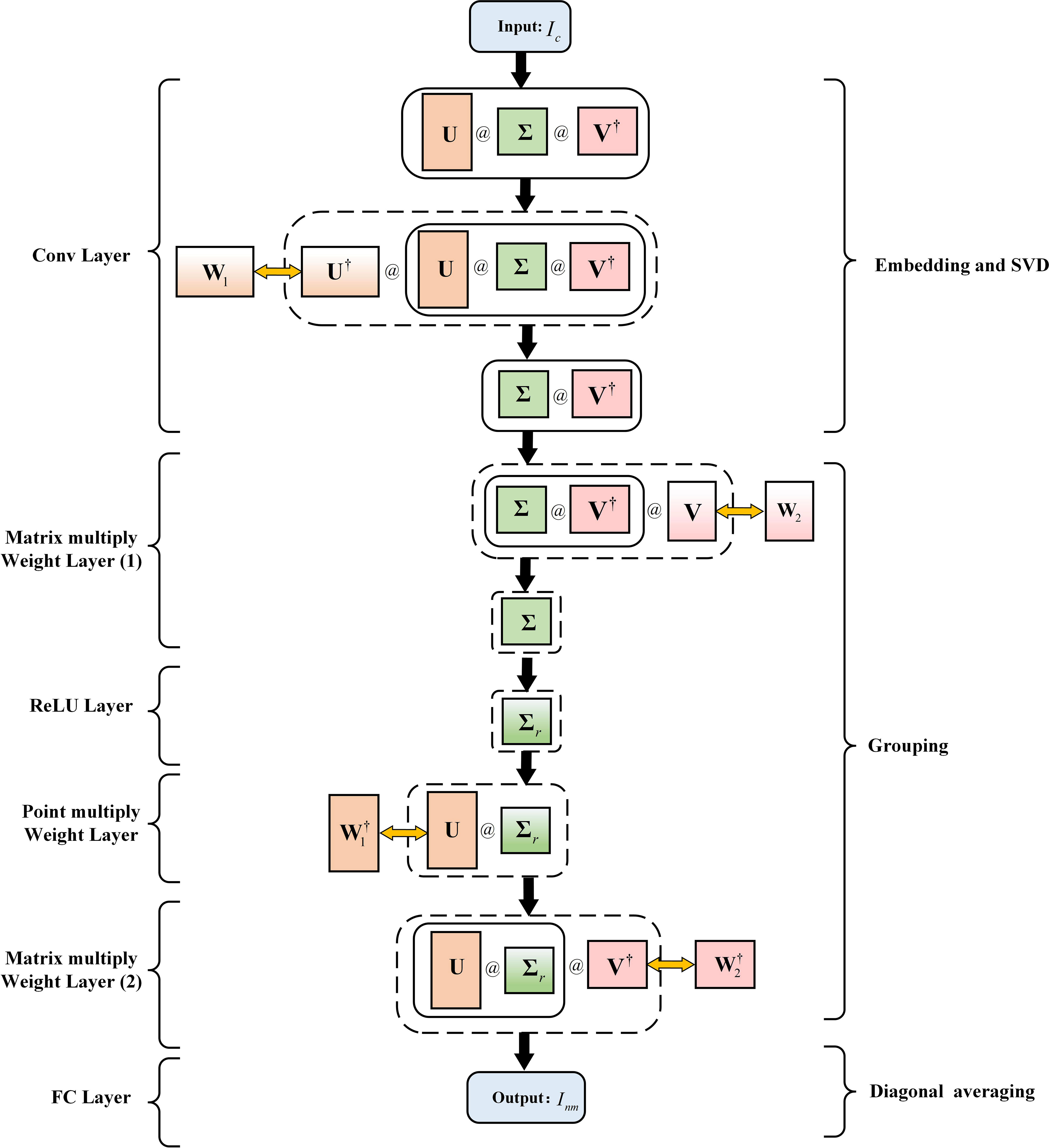
Figure 1 The process of SSA algorithm-unrolled and the corresponding with SSANet, where the input I_c is the received sound interference spectrum, and the output I_nm is the NMIS. W₁, W₂, W${}_1^{†}$, W${}_2^{†}$ are the network parameters of SSANet, U, U^†, V, V^†, Σ, and Σ_r are the matrices of the SSA algorithm unrolled. The symbol ‘@’ represents the matrix multiplication.

1. The SSA algorithm transforms the I_c into the Hankel matrix H and then through SVD to obtain matrix UΣV^†. Next, the matrix UΣV^† left-multiplies the conjugate transpose matrix U^† to obtain the matrix ΣV^†. For SSANet, this process was implemented using a one-dimensional convolutional neural network. As is well known, the output of a one-dimensional convolutional operation with a single channel and one-step is denoted as shown in Equation 10:

where y^′ and y^′′ represent the input and output, respectively, of the convolutional neural layer. Ker is the convolution kernel, (1,v) is the coordinate of Ker, (1,e) is the coordinate of the output vector, and b₁ is the bias. Therefore, b₁ can be initialized to 0, and the above process uses a convolution network implementation. The weight parameter W₁ of the convolutional network corresponds to U^†. The channel number of the convolutional network is equal to the number of rows (R) in matrix U^†, and the size of the Ker is equal to the number of columns (L) in U^†. The output of this convolution operation is equal to matrix ΣV^†. This layer is called the convolutional layer (Conv Layer);

2. In the SSA algorithm, the matrix ΣV^† right-multiplies the matrix V to obtain the singular value matrix Σ. For SSANet, a learnable weight W₂ is used instead of V, and the dimensions of W₂ correspond to the dimensions of V. In this case, each row of the output from the Conv layer matrix-multiplies each column of W₂ to simulate obtaining the singular values in the singular value matrix Σ. This layer is called the matrix multiply weight layer.

3. The SSA algorithm obtains Σ_r by setting the singular values in Σ, except for the first r value of 0. The activation function ReLU (Agarap, 2018) of the neural network satisfies $\mathrm{ReLU}(x)=\{\begin{array}{c}x,x\ge 0\\ 0,x<0\end{array}$. For SSANet, the ReLU activation function can be used to simulate the above process, and this layer is called the ReLU Layer. It should be noted that before using ReLU activation, the singular values are added to a set of learnable bias parameters. Even if the singular values (e.g., the last several values) are larger than zero, they can be filtered out by combining suitable biases through the ReLU layer.

4. In the SSA algorithm, matrix Σ_r left-multiplies the matrix U to obtain UΣ_r. For SSANet, the conjugate transpose of the weight parameter W₁, denoted as ${\mathbf{\text{W}}}_1^{†}$, was used instead of U. The dimensions of ${\mathbf{\text{W}}}_1^{†}$ correspond to the dimensions of U. The output of the ReLU layer was expanded in dimension by copying. Point multiplication is then performed with the weight ${\mathbf{\text{W}}}_1^{†}$ to simulate the process of obtaining UΣ_r. This layer is called the point multiply weight layer.

5. In the SSA algorithm, the matrix UΣ_r right-multiplies the matrix V^† to obtain $\mathbf{\text{A}} \mathbf{=} \mathbf{\text{U}}{\mathbf{\Sigma }}_{\mathit{r}}{\mathbf{\text{V}}}^{\mathbf{†}}$. For SSANet, the network parameters of this layer are replaced by the conjugate transpose of weight parameter W₂ from the second layer, denoted as ${\mathbf{\text{W}}}_2^{†}$. The dimensions of ${\mathbf{\text{W}}}_2^{†}$ correspond to the dimensions of V^†. The output of the previous layer is matrix multiplied by the weight ${\mathbf{\text{W}}}_2^{†}$ simulating obtaining $\mathbf{\text{A}} \mathbf{=} \mathbf{\text{U}}{\mathbf{\Sigma }}_{\mathit{r}}{\mathbf{\text{V}}}^{\mathbf{†}}$. This layer is referred to as the matrix multiply weight layer. In other words, the process of constructing the Hankel matrix, SVD, and grouping to obtain the I in the SSA algorithm is unrolled into the above five steps, corresponding to the five layers in the SSANet neural network.

6. The fourth step in SSA algorithm is diagonal averaging. The process of a fully connected layer in a neural network is represented as $F\text{'}=F\mathbf{\text{W}}+{\mathbf{\text{b}}}_2$ (where F and $F\text{'}$ represent the input and output of the fully connected layer, respectively. W and b₂ are the weight and bias parameters of the fully connected layer, respectively). W and b₂ can achieve data dimensionality reduction and learn complex mapping relations in data through training. Therefore, SSANet implements diagonal averaging with a fully connected network and extracts NMIS by setting the number of output neurons. This layer is referred to as the FC layer.

$\begin{array}{ll}{{\mathbf{y}}^{″}}_{(1,e)}=\sum _{v=1}^V({{\mathbf{y}}^{\prime }}_{(1,e+v-1)}·Ke{r}_{(1,v)})+{\mathbf{b}}_1& (10)\end{array}$

3.2 The structure of SSANet

Based on the unrolling of the SSA algorithm mentioned above, we designed a six-layer network structure called SSANet. Assuming the input is the received and normalized ${\overline{I}}_c\in {ℝ}^{1\times N}$, which undergoes SVD in the SSA algorithm to obtain the unitary matrices $\mathbf{\text{U}}\in {ℝ}^{L\times R}$ and ${\mathbf{\text{V}}}^{†}\in {ℝ}^{R\times K}$, and the singular value matrix $\mathbf{\Sigma }\in {ℝ}^{R\times R}$. The structure of SSANet is illustrated in Figure 2 (the parameters of the SSA algorithm are shown in Figure 2). The dimensions of the network input, weight, and output parameters for each layer are presented in Table 1. The specific steps are as follows:

1. Conv Layer: The number of channels is R, the convolutional kernel size is L, and the step is 1. The output dimension obtained after the convolution operation was R × (N + 1 − L) = R × K (the weight parameter of the Conv layer was ${\mathbf{\text{W}}}_1\in {ℝ}^{R\times L}$).

2. Matrix multiply weight layer (1): Each row of the output R × K of the Conv layer matrix multiplies each column of the weight matrix ${\mathbf{\text{W}}}_2\in {ℝ}^{K\times R}$, and the output dimension is 1 × R.

3. ReLU Layer: Add the previous layer’s output to the bias and use the ReLU function to activate; the output dimension is 1 × R.

4. Point multiply weight layer: Expand the output dimension 1 × R of the ReLU layer to L × R by copying. Then, each column of L × R point multiplies each column of weight ${\mathbf{\text{W}}}_1^{†}\in {ℝ}^L{}^{\times R}$, and the output dimension size is L × R.

5. Matrix multiply weight layer (2): The output L × R of the previous layer right-multiplies the weight ${\mathbf{\text{W}}}_2^{†}\in {ℝ}^{R\times K}$, and the output dimension is L × K.

6. Fc Layer: The output L × K from the previous layer is flattened to 1 × (L × K). The Fc layer results in an output dimension of 1 × (N × num) (where num represents the number of NMIS), thus obtaining the predicted output ${\widehat{I}}_{nm}\in {ℝ}^{1\times (N\times num)}$ of the network.

Figure 2

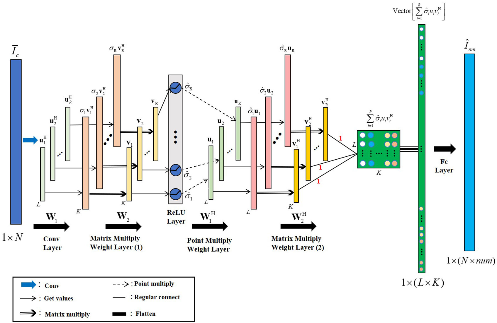
Figure 2 The structure of SSANet.

Table 1

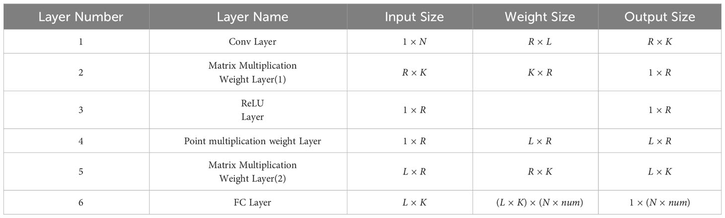
Table 1 The parameters of SSANet.

The implementation of SSANet was carried out using Pytorch 1.6.0, with an NVIDIA Quadro GV100 GPU. The weight parameters W₁ and W₂ were initialized with Kaming initialization (He et al., 2015). The mean absolute error was selected as the loss function and optimized using the Adam optimizer (Kingma and Ba, 2014), with the learning rate (Smith, 2017) set to 1e−4. The batch size was set as 128. To prevent network overfitting, an early stop strategy was adopted in training; the network training was stopped when the loss on the validation set did not drop within 10 epochs (Liang et al., 2019).

4 Simulation and results

In this study, we simulated two canonical ocean waveguides and evaluated the extraction results of each method. In this section, the first part presents the datasets. The second part describes the evaluation criteria for comparing SSANet with other methods, such as FT, MUSIC, and SSA. Finally, an analysis of the results obtained using each method is presented.

4.1 Datasets

This study utilizes the typical sound field simulation software Kraken (Porter, 1992), which is used to simulate typical winter (isovelocity) and summer (thermocline) waveguide sound speed profiles. The sound speed and medium parameters are shown in Figures 3A, B. In these two waveguide environments, the emission frequencies of the sound source were f ∈ [300,360] Hz and f ∈ [180,220] Hz, respectively. The frequency resolution are 0.3 Hz and 0.2 Hz, respectively. It is assumed that the depths of the known hydrophones are 15 m and 30 m, respectively, whereas the depths and distances of the sound sources are unknown.

Figure 3

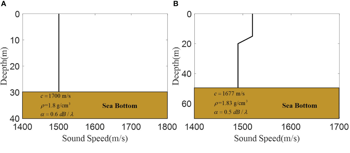
Figure 3 The sound speed and medium parameters. (A) Is the isovelocity waveguide sound speed profiles. (B) Is the thermocline waveguide sound speed profiles.

For the training samples in the isovelocity waveguide, the depth of the sound source was set as z_s = {1,2,…,30} m. At each source depth, 500 data points were randomly generated within the distance r ∈ [10,15] km. A total of 15,000 samples are generated. Similarly, in the thermocline waveguide, the depth of the sound source was set as z_s = {1,2,…,50} m. At each source depth, 500 data points were randomly generated within r ∈ [20,25] km. In total, 25,000 samples were collected. The two training samples are randomly added with noise at SNR = [−10,10] dB and are divided into training and validation sets in an 8:2 ratio for network training. It should be noted that the SSANet model in this study can extract multiple pairs of NMIS by setting the value of num. In this study, we use the extraction of two pairs of NMIS as an example to introduce the SSANet method. Therefore, for the training set, the true labels are the first two pairs of NMIS with larger interference amplitudes, i.e., num = 2 in the SSANet.

According to the method based on Gao et al. (2021), in an isovelocity environment, when z_r= 17 m, z_s= 7 m, and r = 13 km, the singular value distribution of I is shown in Figure 4A. In a thermocline environment, when z_r= 30 m, z_s= 29 m, and r = 23 km, the singular value distribution of I is shown in Figure 4B. As can be seen in Figure 4, there are two large singular values, corresponding to the 1st–3rd NMIS(I₁₃) and the 1st–2nd NMIS (I₁₂). Based on the method for determining the effective rank r in this study, it is known that only two sets of NMIS dominate in the above environment. Therefore, a test set was generated at the aforementioned sound source depth. The isovelocity waveguide set z_r= 17 m, z_s= 7 m, and r = {10,10.025,10.5,…,15} km, and the thermocline waveguide set z_r= 30 m, z_s= 29 m, and r = {20,20.025,20.5,…,25} km. Each of them generates 201 data, which are added to the noise of SNR = [−10,10] dB with an interval of 2 dB, serving as the test set. The datasets used are presented in Table 2. In the data preprocessing stage, all the above data samples were normalized using maximum value normalization.

Figure 4

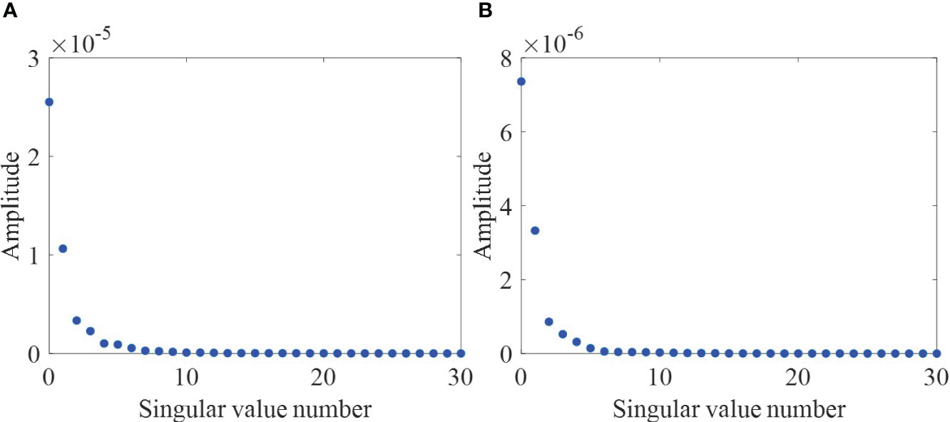
Figure 4 The distribution of singular value. (A) Is the distribution of singular value in the isovelocity waveguide. (B) Is the distribution of singular value in the thermocline waveguide.

Table 2

Table 2 The datasets.

4.2 Evaluation criteria

The root-mean-square error (RMSE) and Mean Absolute Error (MAE) were used to evaluate the performance of the methods. A smaller value for both metrics indicates a minor error between the true and predicted values, indicating better extraction of the NMIS. RMSE and MAE are defined in Equation 11 and Equation 12, as follows:

$\begin{array}{ll}\text{RMSE}=\sqrt{\frac{1}{f}{\displaystyle \sum _{i=1}^f}{\left({\widehat{I}}_{nm}({\omega }_i)-{\overline{I}}_{\text{nm}}({\omega }_i)\right)}^2}& (11)\end{array}$

$\begin{array}{ll}\text{MAE}=\frac{1}{f}\sum _{i=1}^f\left|{\widehat{I}}_{nm}({\omega }_i)-{\overline{I}}_{nm}({\omega }_i)\right|& (12)\end{array}$

where ${\widehat{I}}_{nm}$ and ${\overline{I}}_{nm}$ represent the predicted and true NMIS, respectively.

4.3 Simulation results

This study compares the SSANet method with the traditional methods: FT, MUSIC, and SSA methods (Gao, 2016). For the SSANet method, we assumed the construction of a Hankel matrix as a square matrix; thus, the network parameters are denoted as $L=K=R=\frac{N+1}{2}$=101. The MAE and RMSE obtained by applying the four mentioned methods for extracting I₁₃ and I₁₂ in the isovelocity waveguide under varying SNR are shown in Figures 5A–D. Similarly, the MAE and RMSE obtained by applying the four methods for extracting I₁₃ and I₁₂ in a thermocline waveguide under varying SNR are shown in Figures 6A–D. In addition, a random sample was selected from the test dataset in both environments. Figure 7 shows the input I_c for the isovelocity and thermocline waveguides. Figures 8A–F, respectively, represent the results of extracting I₁₃ and I₁₂ in the isovelocity waveguide using SSANet compared to other methods. Figures 9A–F, respectively, represent the results of extracting I₁₃ and I₁₂ in the thermocline waveguide using SSANet compared to other methods.

Figure 5

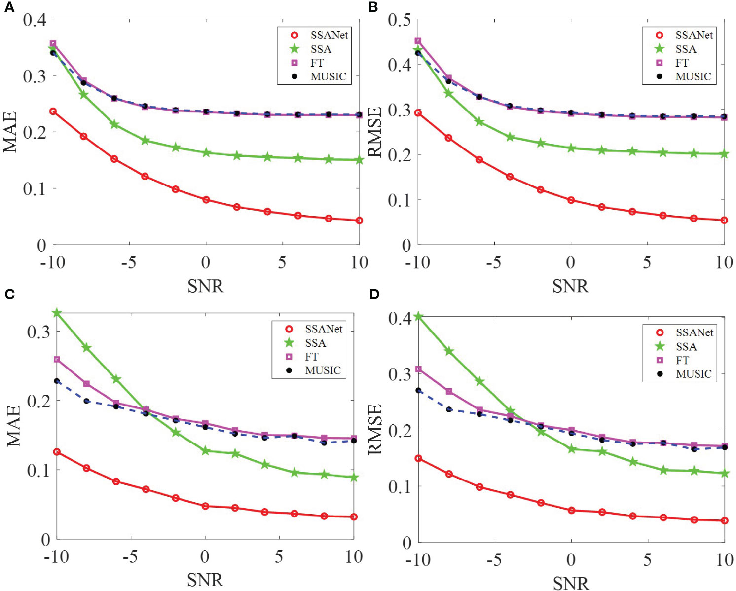
Figure 5 The results of MAE and RMSE in the isovelocity waveguide. (A–D) Represent the MAE and RMSE results of extracting I₁₃ and I₁₂ in the isovelocity waveguide, respectively.

Figure 6

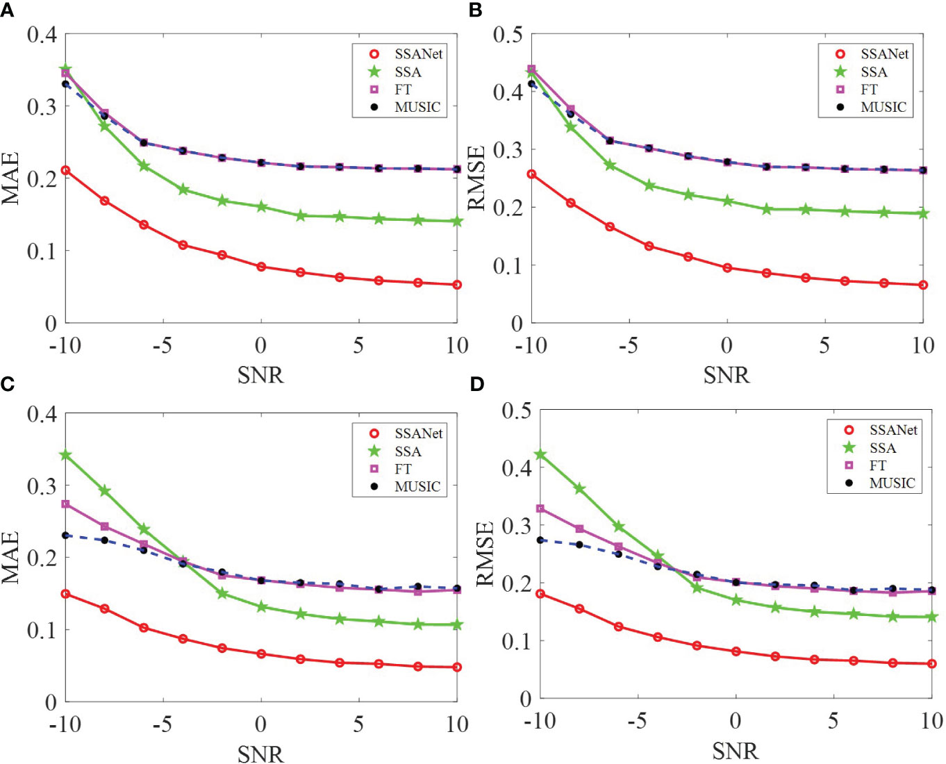
Figure 6 The results of MAE and RMSE in the thermocline waveguide. (A–D) Represent the MAE and RMSE results of extracting I₁₃ and I₁₂ in the thermocline waveguide, respectively.

Figure 7

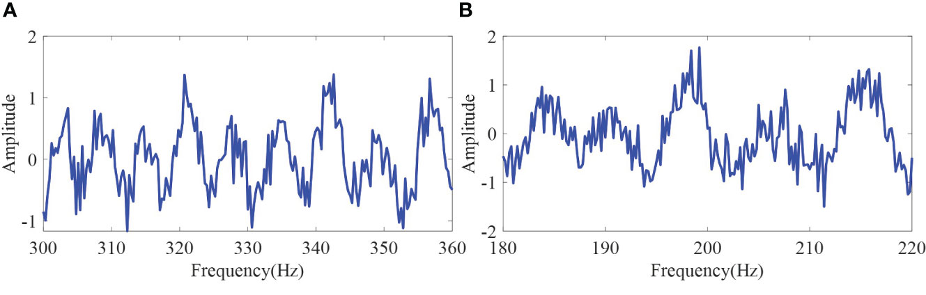
Figure 7 One of the inputs, I_c, of different methods. (A) Represents the input I_c in the isovelocity waveguide. (B) Represents the input I_c in the thermocline waveguide.

Figure 8

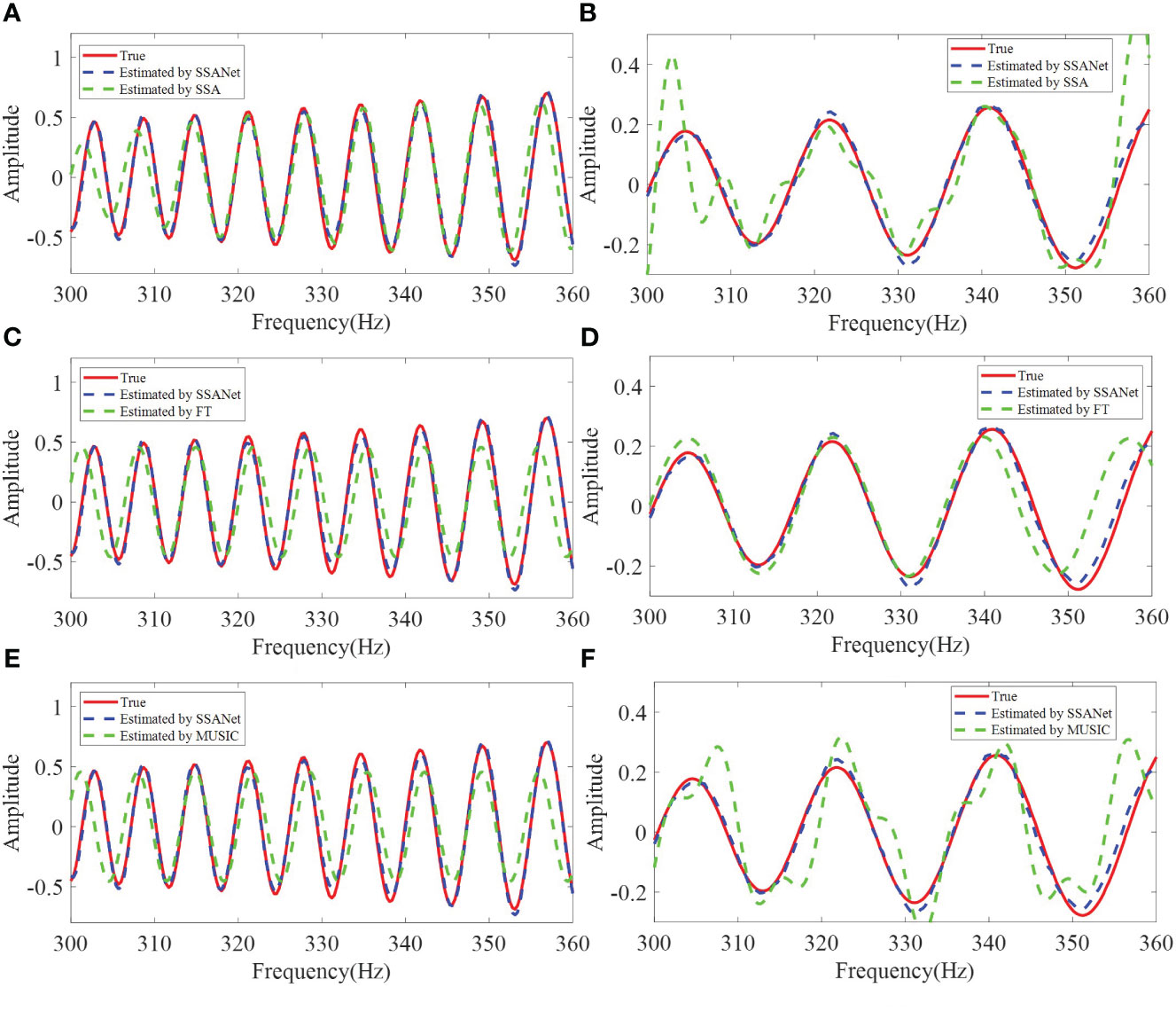
Figure 8 The SSANet extracts I₁₃ result comparing with (A) SSA, (C) FT, and (E) MUSIC from Figure 7A. The SSANet extracts I₁₂ result comparing with (B) SSA, (D) FT, and (F) MUSIC from Figure 7A.

Figure 9

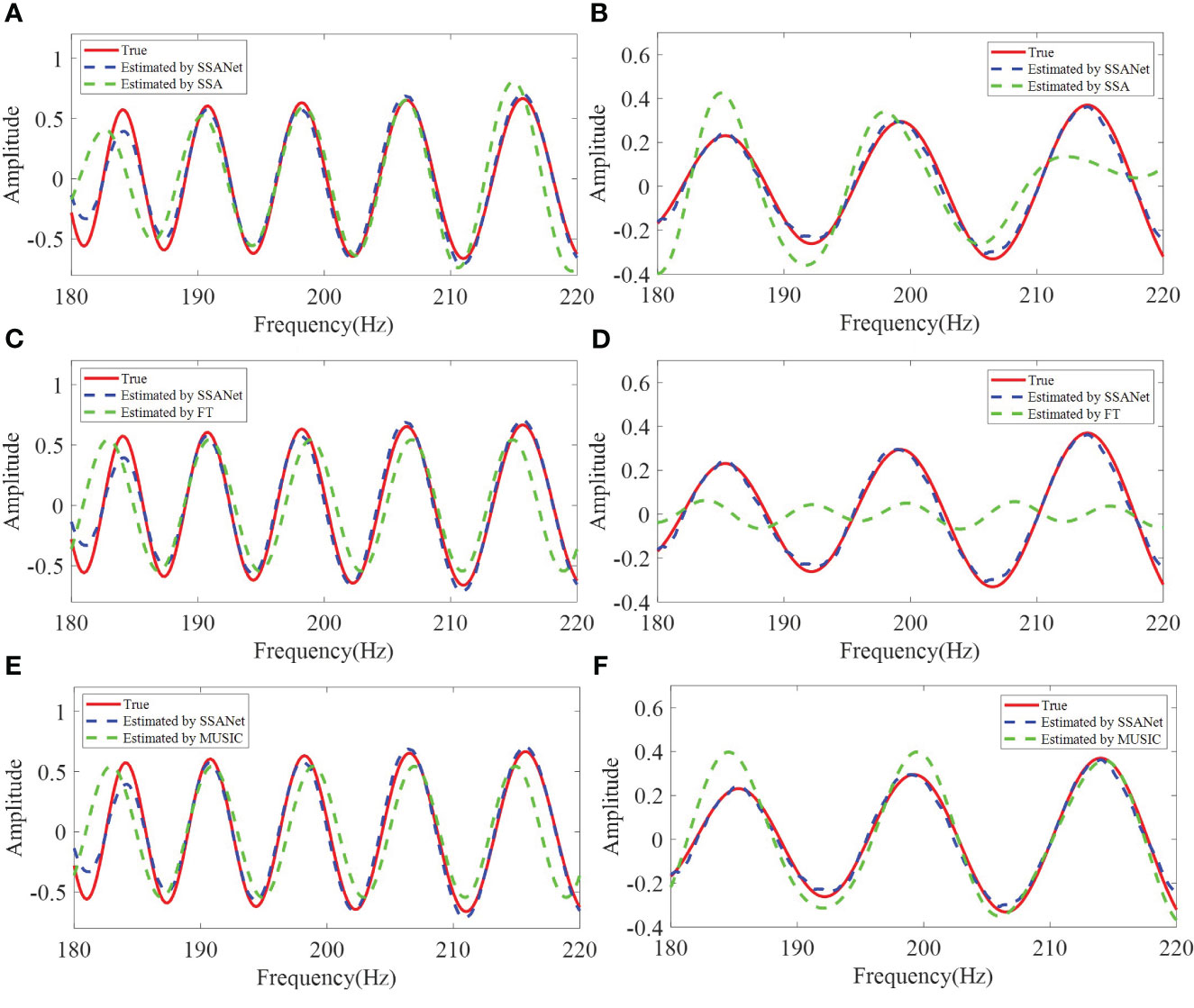
Figure 9 The SSANet extracts I₁₃ result comparing with (A) SSA, (C) FT, and (E) MUSIC from Figure 7B. The SSANet extracts I₁₂ result comparing with (B) SSA, (D) FT, and (F) MUSIC from Figure 7B.

From Figures 5, 6, 8, 9, it can be observed that SSANet provides the overall best extraction results for the phase, amplitude, and oscillation period of the NMIS. However, the FT, MUSIC, and SSA methods exhibit a significant decrease in performance when the amplitude and phase of the NMIS exhibit nonlinear variations with frequency under low SNR conditions. This is because the traditional extraction algorithms are designed by analyzing the physical processes and through handcrafting, while SSANet attempts to automatically discover model information and incorporate NMIS information by optimizing network parameters that are obtained from the training samples (Monga et al., 2021). On the one hand, when there is noise, traditional extraction algorithms do not consider the prior information of the noise, whereas SSANet learns the prior information of the noise during network training, and thus SSANet has stronger noise robustness. On the other hand, when the amplitude and phase of the NMIS exhibit nonlinear changes, the prior assumption of traditional extraction algorithms makes it difficult to extract nonlinear information. The SSANet can learn nonlinear information through training. Overall, it can be said that the trained SSANet is a parameter-optimized version of the SSA algorithm and therefore outperforms traditional extraction algorithms. These results confirm the effectiveness of the SSANet proposed in this study.

5 Conclusion

In this study, a novel algorithm-unrolled neural network model called SSANet was constructed for the extraction of NMIS in lower SNR conditions. The core of the SSANet model is to unroll the SSA algorithm and utilize the powerful data-learning ability of deep learning. The efficiency of the SSANet was validated in different typical ocean waveguides with different SNR. It is found that the SSANet outperformed the traditional FT, MUSIC, and SSA methods at a low SNR. The structure of SSANet is based on the SSA algorithm, and the trained SSANet can be naturally interpreted as a parameter-optimized algorithm, effectively addressing the lack of interpretability in most conventional neural networks. In the future, we will extend the ideas of SSANet to other signal decomposition/extraction problems, which will provide more possibilities for research in this field. Furthermore, the extraction results of NMIS in the ocean waveguide can be applied to sound source localization, waveguide variance estimation, etc.

Data availability statement

The raw data supporting the conclusions of this article will be made available by the authors, without undue reservation.

Author contributions

SZ: Conceptualization, Formal analysis, Methodology, Visualization, Writing – original draft. WG: Methodology, Supervision, Validation, Writing – review & editing. XL: Supervision, Validation, Methodology, Writing – review & editing.

Funding

The author(s) declare financial support was received for the research, authorship, and/or publication of this article. This work was supported by the National Natural Science Foundation of China under Grant Nos. 52071309 and 52001296, the Taishan Scholars under Grant No. tsqn 201909053, and the Fundamental Research Funds for Central Universities under Grant Nos. 202161003, 202065005, 862001013102, 202165007.

Conflict of interest

The authors declare that the research was conducted in the absence of any commercial or financial relationships that could be construed as a potential conflict of interest.

Publisher’s note

All claims expressed in this article are solely those of the authors and do not necessarily represent those of their affiliated organizations, or those of the publisher, the editors and the reviewers. Any product that may be evaluated in this article, or claim that may be made by its manufacturer, is not guaranteed or endorsed by the publisher.

References

Agarap A. F. (2018). Deep learning using rectified linear units (relu). arXiv. doi: 10.48550/arXiv.1803.08375

CrossRef Full Text | Google Scholar

Björck Å. (1990). Least squares methods. Handb. numerical Anal. 1, 465–652. doi: 10.1016/S1570-8659(05)80036-5

CrossRef Full Text | Google Scholar

Fishler E., Grosmann M., Messer H. (2002). Detection of signals by information theoretic criteria: General asymptotic performance analysis. IEEE Trans. Signal Process. 50, 1027–1036. doi: 10.1109/78.995060

CrossRef Full Text | Google Scholar

Gao W. (2016). Singular value decomposition extraction method for simple positive wave coherent components in shallow sea waveguides. Acta Acustica 1, 42–48. doi: 10.15949/j.cnki.0371-0025.2016.01.005

CrossRef Full Text | Google Scholar

Gao W., Li X., Wang H. (2020). Multi-resolution estimation of the interference spectrum per pair of modes in the frequency domain. J. Acoustical Soc. America 148, EL340–EL346. doi: 10.1121/10.0002136

CrossRef Full Text | Google Scholar

Gao W., Wang S., Li X. (2021). Fpm-β: A method for waveguide invariant estimation using one-dimensional broadband acoustic intensity. JASA Express Lett. 1 (8), 084802. doi: 10.1121/10.0005842

PubMed Abstract | CrossRef Full Text | Google Scholar

Grachev G. (1993). Theory of acoustic field invariants in layered waveguides. Acoustical Phys. 39, 33–35.

Google Scholar

Gregor K., LeCun Y. (2010). “Learning fast approximations of sparse coding,” in Proceedings of the 27th international conference on international conference on machine learning. 399–406.

Google Scholar

Hassani H. (2007). Singular spectrum analysis: methodology and comparison. 5, 239–257.

Google Scholar

He K., Zhang X., Ren S., Sun J. (2015). “Delving deep into rectifiers: Surpassing human-level performance on imagenet classification,” in Proceedings of the IEEE international conference on computer vision. 1026–1034.

Google Scholar

Hershey J. R., Roux J. L., Weninger F. (2014). Deep unfolding: Model-based inspiration of novel deep architectures. arXiv preprint arXiv:1409.2574. doi: 10.48550/arXiv.1409.2574

CrossRef Full Text | Google Scholar

Jensen F. B., Kuperman W. A., Porter M. B., Schmidt H., Tolstoy A. (2011). Computational ocean acoustics. 2011. (New York: Springer).

Google Scholar

Kalantari M., Hassani H., Sirimal Silva E. (2020). Weighted linear recurrent forecasting in singular spectrum analysis. Fluctuation Noise Lett. 19, 2050010. doi: 10.1142/S0219477520500108

CrossRef Full Text | Google Scholar

Kingma D. P., Ba J. (2014). Adam: A method for stochastic optimization. arXiv. doi: 10.48550/arXiv.1412.6980

CrossRef Full Text | Google Scholar

LeCun Y., Bengio Y. (1995). Convolutional networks for images, speech, and time series. Handb. Brain Theory Neural Networks 3361 (10), 1995.

Google Scholar

Li B., Zhang L., Zhang Q., Yang S. (2019). An eemd-based denoising method for seismic signal of high arch dam combining wavelet with singular spectrum analysis. Shock Vibration 2019. doi: 10.1155/2019/4937595

CrossRef Full Text | Google Scholar

Liang H., Zhang S., Sun J., He X., Huang W., Zhuang K., et al. (2019). Darts+: Improved differentiable architecture search with early stopping. arXiv. doi: 10.48550/arXiv.1909.06035

CrossRef Full Text | Google Scholar

Lin C., Wu Y. (2022). Singular spectrum analysis for modal estimation from stationary response only. Sensors 22, 2585. doi: 10.3390/s22072585

PubMed Abstract | CrossRef Full Text | Google Scholar

Mallat S. (2016). Understanding deep convolutional networks. Philos. Trans. R. Soc. A: Mathematical Phys. Eng. Sci. 374, 20150203. doi: 10.1098/rsta.2015.0203

CrossRef Full Text | Google Scholar

Monga V., Li Y., Eldar Y. C. (2021). Algorithm unrolling: Interpretable, efficient deep learning for signal and image processing. IEEE Signal Process. Magazine 38, 18–44. doi: 10.1109/MSP.2020.3016905

CrossRef Full Text | Google Scholar

Porter M. B. (1992). The kraken normal mode program (La Spezia, Italy: SACLANT Undersea Research Centre).

Google Scholar

Smith L. N. (2017). “Cyclical learning rates for training neural networks,” in 2017 IEEE winter conference on applications of computer vision (WACV) (IEEE). 464–472.

Google Scholar

Unnikrishnan P., Jothiprakash V. (2022). Grouping in singular spectrum analysis of time series. J. Hydrologic Eng. 27, 06022001. doi: 10.1061/(ASCE)HE.1943-5584.0002198

CrossRef Full Text | Google Scholar

Vautard R., Yiou P., Ghil M. (1992). Singular-spectrum analysis: A toolkit for short, noisy chaotic signals. Physica D: Nonlinear Phenomena 58, 95–126. doi: 10.1016/0167-2789(92)90103-T

CrossRef Full Text | Google Scholar

Wax M., Kailath T. (1985). Detection of signals by information theoretic criteria. IEEE Trans. acoustics speech Signal Process. 33, 387–392. doi: 10.1109/TASSP.1985.1164557

CrossRef Full Text | Google Scholar

Zhao Z. (2010). Research on shallow sea acoustic field interference structure and broadband sound source ranging (China: Ocean University of China).

Google Scholar

Zhao Z., Wang N., Gao D., Wang H. (2010). Broadband source ranging in shallow water using the Ω-interference spectrum. Chin. Phys. Lett. 27, 064301. doi: 10.1088/0256-307X/27/6/064301

CrossRef Full Text | Google Scholar