A simplified decision feedback Chebyshev function link neural network with intelligent initialization for underwater acoustic channel equalization

Introduction: In shallow-water environments, the reliability of underwater communication links is often compromised by significant multipath effects. Some equalization techniques such as decision feedback equalizer, and deep neural network equalizer suffer from slow convergence and high computational complexity.

Methods: To address this challenge, this paper proposes a simplified decision feedback Chebyshev function link neural network equalizer (SDF-CFLNNE). The structure of the SDF-CFLNNE employs Chebyshev polynomial function expansion modules to directly and non-linearly transform the input signals into the output layer, without the inclusion of hidden layers. Additionally, it feeds the decision signal back to the input layer rather than the function expansion module, which significantly reduces computational complexity. Considering that, in the training phase of neural networks, the random initialization of weights and biases can substantially impact the training process and the ultimate performance of the network, this paper proposes a chaotic sparrow search algorithm combining the osprey optimization algorithm and Cauchy mutation (OCCSSA) to optimize the initial weights and thresholds of the proposed equalizer. The OCCSSA utilizes the Piecewise chaotic population initialization and combines the exploration strategy of the ospreywith the Cauchy mutation strategy to enhance both global and local search capabilities.

Rseults: Simulations were conducted using underwater multipath signals generated by the Bellhop Acoustic Toolbox. The results demonstrate that the performance of the SDFCFLNNE initialized by OCCSSA surpasses that of CFLNN-based and traditional nonlinear equalizers, with a notable improvement of 2-6 dB in terms of signal-to-noise ratio at a bit error rate (BER) of 10−4 and a reduced mean square error (MSE). Furthermore, the effectiveness of the proposed equalizer was validated using the lake experimental data, demonstrating lower BER and MSE with improved stability.

Discussion: This underscores thepromise of employing the SDFCFLNNE initialized by OCCSSA as a promising solution to enhance the robustness of underwater communication in challenging environments.

1 Introduction

The shallow water acoustic environment is complex and changeable, which often exhibits intricate signal multipath effects and Doppler frequency shifts (Stojanovic and Preisig, 2009; Huang et al., 2018). The multipath propagation of underwater acoustic (UWA) signals originates from the effects of acoustic boundaries (such as reflection from the water surface and seabed), refraction caused by the non-uniformly distributed dissound speed in the water, as well as scattering from particles. The complex multipath results in significant signal time spreading, thereby causing severe intersymbol interference. In typical shallow water acoustic communications, intersymbol interference may span over hundreds of symbols. Consequently, at the receiver end, it is essential for the channel equalization to possess strong adaptive channel tracking capabilities (Song et al., 2006; Wang et al., 2021). This poses a significant challenge for reliable and efficient UWA communication (Zhang et al., 2018).

To combat intersymbol interference caused by time-varying multipath propagation, extensive research has been conducted on various channel equalization techniques. Single-carrier schemes and time-domain equalization techniques offer high spectral efficiency and robustness, albeit at the cost of high receiver complexity (Stojanovic and Preisig, 2009; Zhang et al., 2018). The proposed adaptive step-size least mean square performs well for many channel types, but for certain complex non-stationary UWA channels, the rapid tracking capability of recursive least square is essential (Freitag et al., 1997). To achieve reliable coherent communication over UWA channels, a receiver was designed which combines the recursive least square algorithm with a second-order digital phase-locked loop for carrier synchronization and performs fractionally spaced decision feedback equalization of the received signals. The parameters of this receiver are adaptively adjusted (Stojanovic et al., 1994). An adaptive nonlinearity (piecewise linear) was introduced into the channel equalization algorithm and its effectiveness was demonstrated through highly realistic experiments conducted on real-field data as well as accurate simulations of UWA channels (Kari et al., 2017). In recent years, in order to alleviate propagation errors, expedite convergence speed, and further enhance receiver performance, there has been growing research on adaptive turbo equalization (He et al., 2019; Xi et al., 2019; Qin et al., 2020). Considering the sparsity inherent in UWA channels, sparse matrices have been utilized to construct sparse equalizers, aiming to achieve faster convergence and lower error rates (Xi et al., 2020; Wang et al., 2021; Wang et al., 2021). Additionally, the equalization challenges in an impulsive interference single-carrier modulation system based on a parameterized model are addressed, and a two-step equalization algorithm is proposed (Ge et al., 2022). The robust equalization for single-carrier underwater acoustic communication in sparse impulsive interference environment was proposed (Wei et al., 2023). This algorithm is based on the framework of variational Bayesian inference and possesses the unique capability of simultaneously accounting for the sparsity inherent in the channel and impulse interference. At the same time, several waveform design (Zhu et al., 2023) and enhanced receiver schemes (Zhang et al., 2021; Liu et al., 2023) were proposed to further address inter-symbol interference and multipath propagation issues. However, the complex multipath effect of the UWA channels contributes to the slow convergence rate and extensive computational requirements of traditional equalization algorithms. As a result, there is substantial room for improvement in UWA communication systems.

In recent years, machine learning techniques have garnered attention across various fields. Particularly, deep learning (DL) technology holds tremendous potential for addressing non-parametric problems such as object detection and recognition (Tsai et al., 2013), speech recognition (Zhang and Wang, 2016), target tracking (Milan et al., 2017), wireless communication (Wang et al., 2017; Ma et al., 2018; van Heteren, 2022; Mishra et al., 2023). In order to reduce the computational costs of traditional equalizers, machine learning-based equalizers have been introduced to mitigate intersymbol interference. Channel equalization can be viewed as a classification problem, where the equalizer is designed as a decision device with the motivation to classify the transmitted signals as accurately as possible (Zhang and Yang, 2020). Gibson et al. introduced an adaptive equalizer employing a neural network architecture based on multilayer perceptrons (MLP) to counter intersymbol interference on linear channels with Gaussian white noise (Gibson et al., 1989). Chang et al. proposed a neural network-based decision feedback equalizer (DFE) that obviates the need for time-consuming complex-valued backpropagation training algorithms (Chang and Wang, 1995). Gao et al. demonstrated that in underwater digital communication scenarios, their proposed blind equalizer achieves faster convergence speed and smaller mean square error (MSE) compared to original MLP-based equalizers that require training data (Gao et al., 2009). Zhang et al. proposed a DL-based time-varying UWA channel single-carrier communication receiver to adapt to the dynamic characteristics of UWA channels. The receiver operates in an alternating mode between online training and testing (Zhang et al., 2019b). Zhang et al. introduced a DL-based UWA communication orthogonal frequency-division multiplexing receiver. A stack of convolutional layers with skip connections effectively extracts meaningful features from the received signal and reconstructs the original transmitted symbols (Zhang et al., 2022). Radial basis function (RBF) neural networks have garnered the attention of many researchers due to their simple structure and high learning efficiency, and have been utilized for addressing channel equalization issues (Lee and Sankar, 2007; Guha and Patra, 2009; Ning et al., 2009).

However, with a higher channel order, a greater number of RBF centers are required, ultimately resulting in an excessive computational burden. To overcome these drawbacks of MLP and RBF, another novel single-layer neural network, known as the Functional Link Neural Network (FLNN), was proposed by Paul. Due to the non-linear processing of signals in the FLNN, it can generate arbitrarily complex decision regions (Patra et al., 1999). This network features a simple structure with only input and output layers, and the hidden layer is entirely replaced by non-linear mappings. These mappings are introduced through the expansion of input patterns using trigonometric polynomials and other basis functions like Gaussian polynomials, orthogonal polynomials, Legendre polynomials, and Chebyshev polynomials (Burse et al., 2010). The FLNN increases the dimensionality of the input signal space by a set of linearly independent non-linear functions, thus reducing computational load and allowing for straightforward hardware implementation (Patra et al., 2008; Zhang and Yang, 2020). Moreover, research indicates that non-linear equalizers based on FLNN outperform MLP, RBF, and PPN equalizers in terms of MSE, convergence rate, bit error rate (BER), and computational complexity (Patra et al., 1999). Lee et al. introduced a Chebyshev Neural Network for static function approximation, which is more computationally efficient than trigonometric polynomials when expanding the input space for extended static function approximation and non-linear dynamic system identification (Lee and Jeng, 1998). Patra et al. have employed Chebyshev Functional Link Neural Networks (CFLNN) for channel equalization of four quadrature amplitude modulation signals (Patra and Kot, 2002; Patra et al., 2005). Hussain combined traditional DFE with FLNN, proposing a Decision Feedback Functional Link Neural Network Equalizer (DFFLNN) (Hussain et al., 1997). Building upon this, they introduced a Chebyshev orthogonal polynomial cascaded FLNN for non-linear channel equalization (Zhao and Zhang, 2008) and an adaptive DFE based on the combination of the FIR and FLNN (Zhao et al., 2011). Moreover, Convolutional Neural Network (He et al., 2023), Recurrent Neural Networks (Kechriotis et al., 1994; Chagra et al., 2005; Xiao et al., 2008; Zhao et al., 2010; Li et al., 2021; Qiao et al., 2022), Fuzzy Neural Networks (Heng et al., 2006; Chang and Ho, 2009; Chang and Ho, 2011), Extreme Learning Machines (Yang et al., 2018; Liu et al., 2019), Wavelet Neural Networks (Xiao and Dong, 2015), Support Vector Machines (Zhang et al., 2019a), other neural network models and Deep Reinforcement Learning (He and Tao, 2023) have been employed for channel equalization.

Swarm intelligence optimization algorithms are a class of bio-inspired algorithms inspired by the behavioral patterns of certain social organisms in the natural world. The central idea is to conduct both global and local searches within a solution space to find optimal solutions. These algorithms provide a new approach to solving complex problems without centralized control or a global model. In recent years, new swarm intelligence optimization algorithms have continuously emerged. Scholars have drawn inspiration from the behavior of various animals such as ants, wolves, birds, moths, whales, sparrows, and more to propose a series of swarm intelligence optimization algorithms, including the Particle Swarm Optimization (PSO) algorithm (Kennedy and Eberhart, 1995), the Grey Wolf Optimization (GWO) algorithm (Mirjalili et al., 2014), the Whale Optimization Algorithm (WOA) (Mirjalili and Lewis, 2016), the Bald Eagle Search (BES) algorithm (Alsattar et al., 2020), the Sparrow Search Algorithm (SSA) (Xue and Shen, 2020), the Cooperation Search Algorithm (CSA) (Feng et al., 2021), artificial gorilla troops optimizer(GTO)(Abdollahzadeh et al., 2021), white shark optimizer(WSO)(Braik et al., 2022), dung beetle optimizer(DBO)(Xue and Shen, 2023) and Osprey Optimization Algorithm(OOA)(Dehghani and Trojovskỳ, 2023). The Sparrow Search Algorithm (SSA) was first introduced by Xue et al. in 2020 (Xue and Shen, 2020). In comparison to other algorithms, SSA offers several advantages, including fast convergence, strong optimization capabilities, and a wider range of application scenarios. As a result, SSA has garnered the attention of researchers from various fields. However, SSA does have limitations in terms of initial population quality, search capabilities, and population diversity. To address these issues, the Improved Sparrow Search Algorithm (ISSA) was proposed (Song et al., 2020). ISSA introduces non-linear decay in the position updates of producers, which facilitates the exploration and utilization of the search space. ISSA incorporates a mutation strategy to update the positions of scavengers with lower energy, combining chaotic search with local development by higher-energy scavengers. This enhances diversity and prevents falling into local optima. At the same time, the Tent mapping is used to initialize the population. Then, for the producers, an adaptive weight strategy is combined with the Levy flight mechanism, making the fusion search approach more comprehensive and flexible. Finally, in the scavenger stage, a variable spiral search strategy is employed to provide a more detailed search scope (Ouyang et al., 2021).

Traditional network equalizers suffer from problems such as large steady-state errors, slow convergence, susceptibility to local minima during the search process, and the curse of dimensionality. Moreover, in the training phase of neural networks, the random initialization of weights and biases can substantially impact the training process and the ultimate performance of the network. In contrast, swarm intelligence optimization algorithms exhibit strong convergence and high precision advantages in the optimization process of practical problems. Therefore, they have become popular research topics in the field of equalizer optimization methods. A modified constant modulus algorithm digital channel equalizer learning algorithm based on PSO is proposed by Sahu (Sahu and Majumder, 2021). The particle swarm algorithm is employed as the training algorithm, resulting in a shorter convergence time and better performance compared to traditional LMS algorithms. This equalizer avoids introducing any phase ambiguity and does not get trapped in local optima. A novel training strategy using the Fuzzy Firefly Algorithm is proposed for channel equalization (Mohapatra et al., 2022). By employing an appropriate network topology and parameters, the suggested training system exhibits enhanced exploration and exploitation capabilities, as well as the ability to address local minima issues. An enhanced Grasshopper Optimization Algorithm (GOA) is proposed for nonlinear wireless communication channel equalization (Ingle and Jatoth, 2023). By combining Levy flights and greedy selection operators with the basic GOA, the diversity of the swarm is increased. Simulation results on four nonlinear channels demonstrate the exploration and exploitation capabilities of the improved Grasshopper Optimization Algorithm in terms of MSE and BER performance. An effective equalizer based on artificial neural networks is proposed by Shwetha (Shwetha et al., 2023). The Battle Royale Optimization method, as introduced, is utilized to train the weights of the neural network. The effectiveness of this approach is demonstrated through the evaluation of performance metrics such as MSE, mean squared residual error, and BER.

In shallow water acoustic propagation, there often exists severe multipath effects. Traditional equalization techniques may require hundreds of taps, greatly increasing system complexity. While the DFFLNNE (Hussain et al., 1997) outperforms FLNNE and traditional DFE, but it increases the dimensionality of the input layer, raising the complexity of the network structure. Simultaneously, during the training phase of the network, random initialization of weights and biases can affect the neural network’s training process and final performance. Improper initialization can lead to problems such as gradient vanishing or exploding, causing training to be infeasible or overly slow. To enhance communication reliability without increasing system complexity, this paper proposes a simplified decision feedback Chebyshev functional link neural network equalizer (SDF-CFLNNE) initialized with swarm intelligence optimization algorithms. The papers contributions can be summarized as follows.

1. To address the issue of unreliability in underwater communication links caused by significant strong multipath effects in shallow-water environments, we propose a simplified decision feedback Chebyshev function link neural network equalizer.

2. To optimize the initial weights and thresholds of the proposed equalizer, We propose a Chaotic Sparrow Search Algorithm combining osprey optimization algorithm and Cauchy mutation. This approach mitigates the instability resulting from random weight initialization in the network equalizer.

The rest of this paper is organized as follows. In Section 2, a novel simplified decision feedback Chebyshev functional link neural network equalizer is proposed to address the unreliability of communication due to multipath effects. In Section 3, a chaotic sparrow search algorithm combining osprey optimization algorithm and Cauchy mutation is proposed for intelligent optimization of network weight and bias initialization. We validate the method through simulation and lake experimental data processing in Section 4. Finally, conclusions are given in Section 5.

2 A novel simplified decision feedback Chebyshev functional link neural network equalizer

2.1 Decision feedback Chebyshev functional link neural network equalizer

To overcome intersymbol interference caused by multipath effects, a channel equalizer is embedded in the receiver to restore the transmitted signal. The FLNNE (Patra et al., 1999) has no hidden layers and is composed solely of a function extension module and a single-layer perceptron. This composition enables the generation of complex decision regions through the creation of nonlinear decision boundaries. In contrast to the linear weighting of input patterns generated by linear connections in MLP, the function expansion module enhances the dimensionality of input patterns by applying a set of linearly independent functions to elements or the entire pattern itself, thus enhancing its representation in high-dimensional space. Moreover, due to its single-layer structure, this FLNN structure exhibits lower computational complexity and faster convergence speed compared to other traditional neural networks. As widely recognized, utilizing the optimal approximation theory, Chebyshev orthogonal polynomials possess a robust capability for nonlinear approximation (Patra et al., 2005). The function expansion module in this context is composed of Chebyshev polynomials and their outer products, serving to simulate nonlinear channels, to construct the Chebyshev Functional Link Neural Network Equalizer (CFLNNE). The Figure 1 illustrates the structure of the CFLNNE.

Figure 1

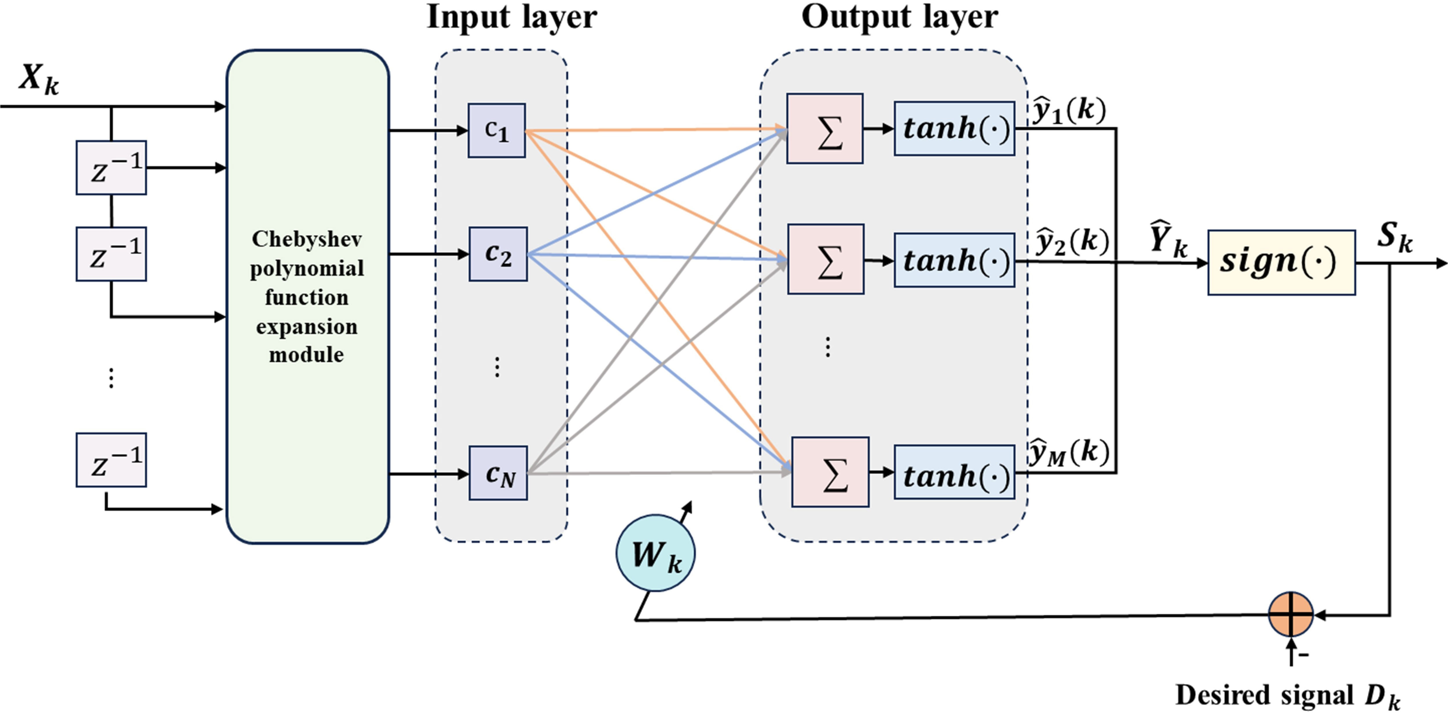
Figure 1 The structural diagram of the CFLNNE.

Chebyshev polynomials are a set of orthogonal polynomials defined as solutions to the Chebyshev differential equation, denoted as T_n(x). Chebyshev polynomials are computationally more tractable compared to trigonometric polynomials. The first several Chebyshev polynomials are given by T₀(x) = 1, T₁(x) = x, and T₂(x) = 2x² − 1. When the input signal is X_k= [x₁(k),x₂(k),…,x_M(k)]^T, the higher-order Chebyshev polynomials for −1< x< 1 can be generated using the following recursion formula Equation 1:

$\begin{array}{ll}\begin{array}{l}{c}_1(X_k)=T_0(X_k)=1,\\ c_2(X_k)=T_1(X_k)=X_k,\\ ⋮\\ c_{n+2}(X_k)=T_{n+1}(X_k)=2X_k{T}_n(X_k)-T_{n-1}(X_k)\end{array}& (1)\end{array}$

In CFLNNE, the input signal denoted as X_k, is expanded into N linearly independent functions using Chebyshev polynomials, and can be represented as C_k= [c₁(X_k)c₂(X_k)…c_N(X_k)]^T.

Through forward propagation, the j-th neuron of the output layer can be represented as Equations 2 and 3:

$\begin{array}{ll}{u}_j(k)={\displaystyle \sum _{i=1}^N{w}_{ji}}(k)c_i(X_k)+b_j(k)i=1,2,\dots ,N;j=1,2,\dots M.& (2)\end{array}$

$\begin{array}{ll}{\widehat{y}}_j(k)=f(u_j(k))=f({\displaystyle \sum _{i=1}^N{w}_{ji}}(k)c_i(X_k)+b_j(k))i=1,2,\dots ,N;j=1,2,\dots M.& (3)\end{array}$

where w represents the weight coefficients from the input layer to the output layer, and b represents the bias of the output layer. The nonlinear activation function here is f(·) = tanh(·), and its derivative is denoted as f′(·).

The output signal after decision device can be represented as Equation 4:

$\begin{array}{ll}s(k)=sign(\widehat{y}(k))=\{\begin{array}{ll}-1\hfill & \text{ if }\widehat{y}(k)<0\hfill \\ 1\hfill & \text{ if }\widehat{y}(k)\ge 0\hfill \end{array}& (4)\end{array}$

Taking advantage of the traditional decision feedback equalizer’s ability to mitigate inter-symbol interference introduced by the preceding information symbol, Hussain et al. integrated the DFE with a FLNN, creating the decision feedback functional link neural network (Hussain et al., 1997). To further enhance the nonlinear approximation capabilities of the function link module, the DFE is combined with CFLNNE to form a decision feedback Chebyshev functional link neural network (DF-CFLNNE), as illustrated in Figure 2.

Figure 2

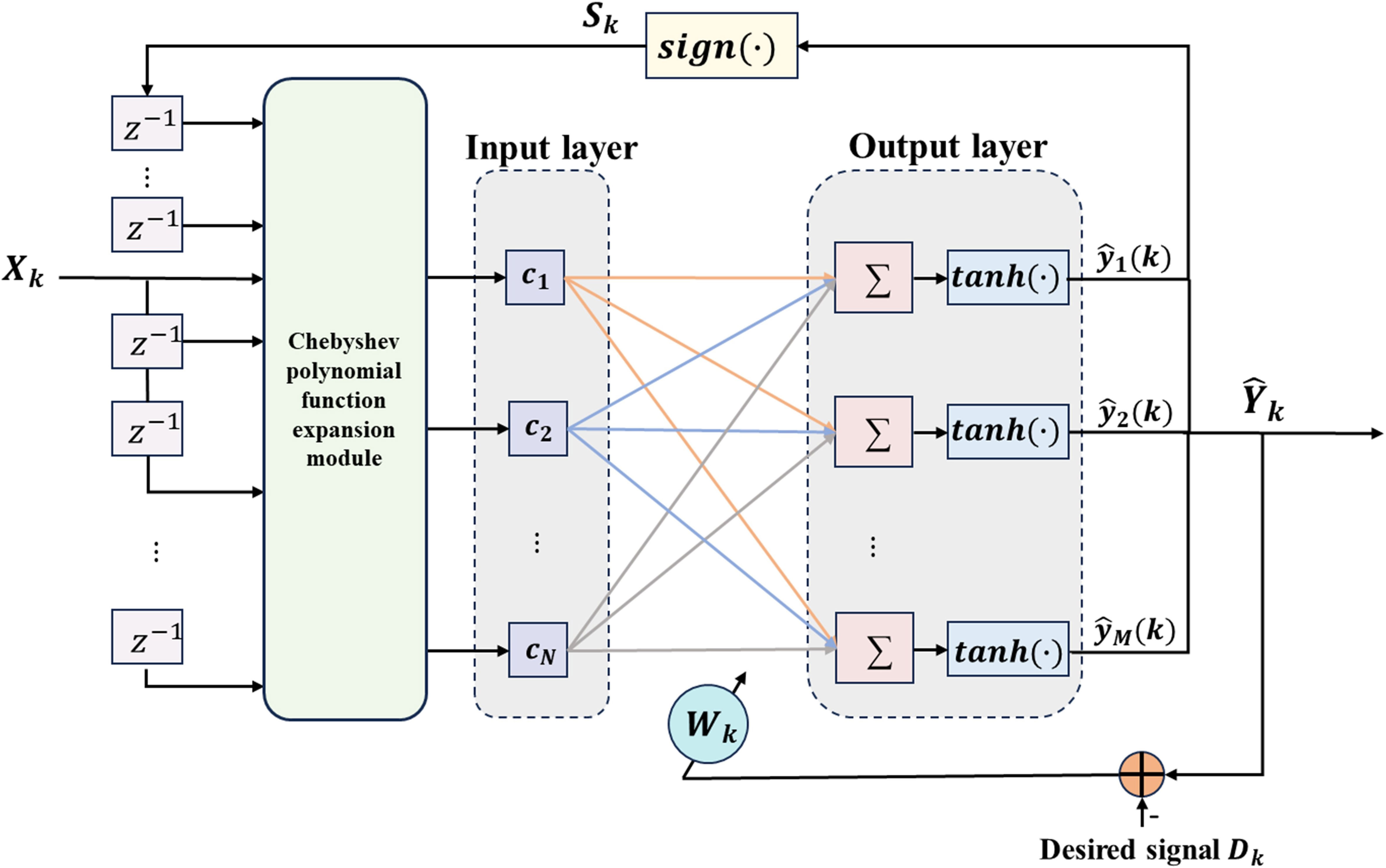
Figure 2 The structural diagram of the DF-CFLNNE.

The input signal X_k= [x₁(k),x₂(k),…,x_M(k)]^T and feedback signal $S_k={[s_1(k),\dots ,s_{N_2}(k)]}^T$ from the decision device are jointly used as the input signal Z_k= [X_k, S_k] for the DF-CFLNNE, where N₂ represents the order of the feedback delay path. The key distinction from CFLNNE is that CFLNNE takes only X_k as its input signal, without the feedback signals from the decision device. Subsequently, the input signal Z_kof DF-CFLNNE is expanded into N linearly independent functions using Chebyshev polynomials, denoted as C_k= [c₁(Z_k),c₂(Z_k),…,c_N(Z_k)]^T, where C_k serves as the input to the network’s input layer.

Through forward propagation, the j-th neuron of the output layer can be represented as Equations 5 and 6:

$\begin{array}{ll}{u}_j(k)={\displaystyle \sum _{i=1}^N{w}_{ji}}(k)c_i(Z_k)+b_j(k)i=1,2,\dots ,N;j=1,2,\dots M.& (5)\end{array}$

$\begin{array}{ll}{\widehat{y}}_j(k)=f(u_j(k))=f({\displaystyle \sum _{i=1}^N{w}_{ji}}(k)c_i(Z_k)+b_j(k))i=1,2,\dots ,N;j=1,2,\dots M.& (6)\end{array}$

For convenience, these values of functions can be represented in matrix form as Equation 7:

$\begin{array}{ll}{\widehat{Y}}_k=f(W_k{C}_k+B_k)& (7)\end{array}$

where W_k is an M ×N dimensional matrix, i.e., W_k= [w_j1,w_j2,…,w_jN]. B_k is an M ×1 dimensional matrix, i.e., B_k= [b₁,b₂,…,b_M]. The output of the entire network can be represented in matrix form as ${\widehat{\mathbf{Y}}}_k={[{\widehat{y}}_1,{\widehat{y}}_2,\dots {\widehat{y}}_M]}^T$.

We use the MSE as the loss function, which can be represented as Equation 8:

$\begin{array}{ll}{J}_k={\displaystyle \sum {({\mathbf{D}}_k-{\widehat{\mathbf{Y}}}_k)}^2}& (8)\end{array}$

where D_k represents the desired output sequence at time instant k.

The backpropagation algorithm is employed here to train the DF-CFLNN. The training process is expressed as follows Equations 9 and 10:

$\begin{array}{ll}\begin{array}{ll}\frac{\text{d}{J}_k}{\text{d}{W}_k}\hfill & =\frac{\partial J_k}{\partial {\widehat{Y}}_k}·\frac{\partial {\widehat{Y}}_k}{\partial U_k}·\frac{\partial U_k}{\partial W_k}\hfill \\ \hfill & =2(D_k-{\widehat{Y}}_k)·f^{\prime }(U_k)·C_k\hfill \\ \hfill & =2(D_k-{\widehat{Y}}_k)·(1-{\widehat{Y}}_k^2)·C_k\hfill \end{array}& (9)\end{array}$

$\begin{array}{ll}\begin{array}{ll}\frac{\text{d}{J}_k}{\text{d}{B}_k}\hfill & =\frac{\partial J_k}{\partial {\widehat{Y}}_k}·\frac{\partial {\widehat{Y}}_k}{\partial U_k}·\frac{\partial U_k}{\partial B_k}\hfill \\ \hfill & =2(D_k-{\widehat{Y}}_k)·f^{\prime }(U_k)\hfill \\ \hfill & =2(D_k-{\widehat{Y}}_k)·(1-{\widehat{Y}}_k^2)\hfill \end{array}& (10)\end{array}$

According to the gradient descent algorithm, there will be Equations 11 and 12:

$\begin{array}{ll}{W}_k=W_k-\mu \frac{\text{d}{J}_k}{\text{d}{W}_k}& (11)\end{array}$

$\begin{array}{ll}{B}_k=B_k-\mu \frac{\text{d}{J}_k}{\text{d}{B}_k}& (12)\end{array}$

where the parameter µ denotes the learning factor.

2.2 Simplified decision feedback Chebyshev functional link neural network equalizer

DF-CFLNNE increases the system’s performance at the cost of increased complexity. In order to reduce hardware costs without compromising system performance, a simplified DF-CFLNNE (SDF-CFLNNE) structure is proposed as illustrated in Figure 3.

Figure 3

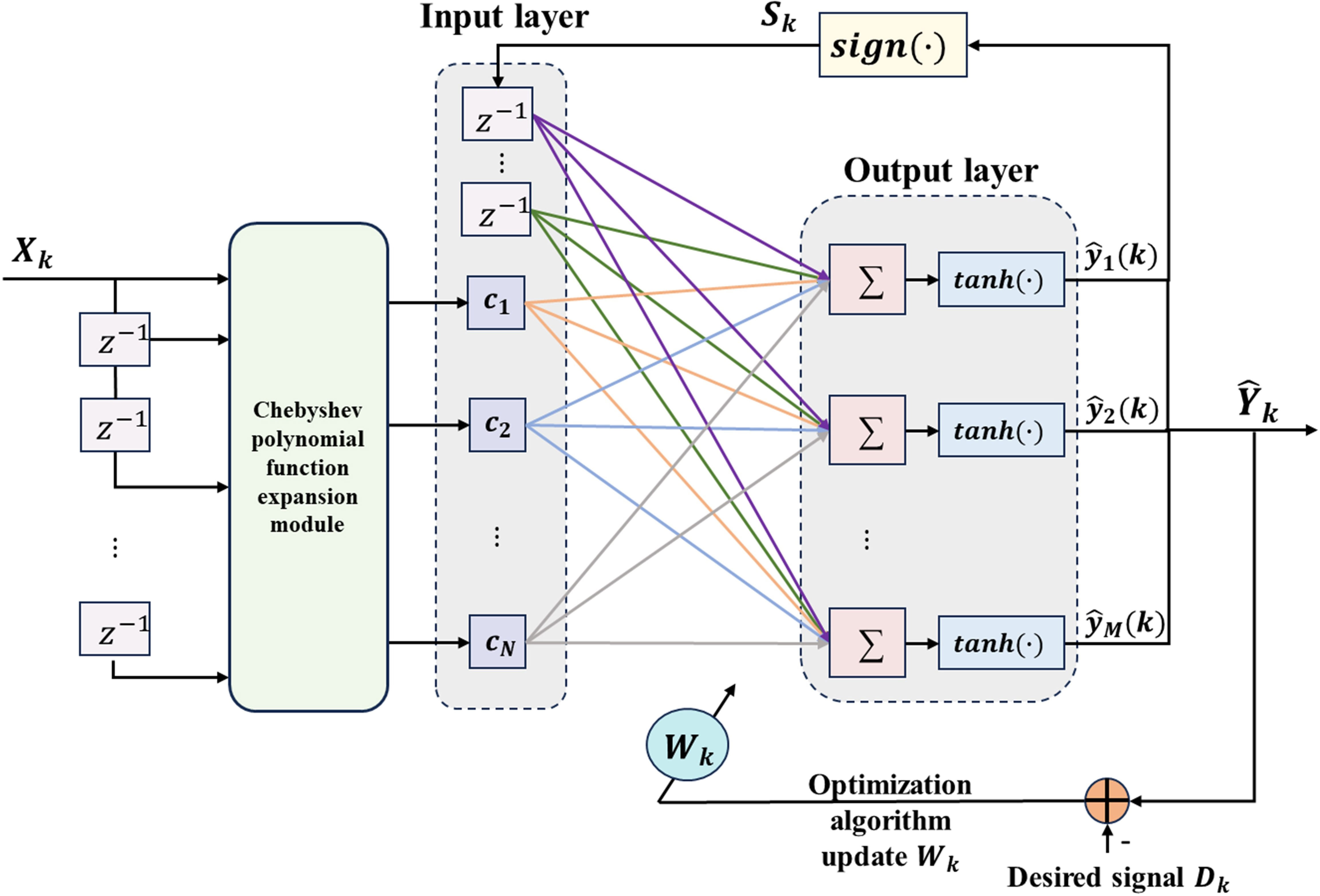
Figure 3 The structural diagram of the SDF-CFLNNE.

In the SDF-CFLNNE structure, the post-decision output signal is directly fed back to the input layer of the neural network, rather than being used as an input signal to the network, and it no longer goes through the function expansion module. Namely, the input layer signal is composed of the Chebyshev polynomial function expansion of the received signal, denoted as C_k= [c₁(X_k),c₂(X_k),…,c_N(X_k)]^T, and the feedback signal fafter decision, denoted as $S_k={[s_1(k),\dots ,s_{N_2}(k)]}^T$, which can be represented as $G_k={[c_1(X_k),c_2(X_k),\dots ,c_N(X_k),s_1(k),\dots ,s_{N_2}(k)]}^T={[g_1(k),\dots ,g_P(k)]}^T,P=N+N_2$. It can be observed from Figures 2, 3 that the number of input signals in SDF-CFLNNE is fewer compared to DF-CFLNNE. Consequently, the number of signals after the function expansion module for SDF-CFLNNE is significantly reduced compared to DF-CFLNNE. This streamlined system structure enhances computational efficiency.

Through forward propagation, the j-th neuron of the output layer can be represented as Equations 13 and 14:

$\begin{array}{ll}{u}_j(k)={\displaystyle \sum _{i=1}^N{w}_{ji}}(k)g_i(k)+b_j(k)i=1,2,\dots ,P;j=1,2,\dots M.& (13)\end{array}$

$\begin{array}{ll}{\widehat{y}}_j(k)=f(u_j(k))=f({\displaystyle \sum _{i=1}^N{w}_{ji}}(k)g_i(k)+b_j(k))i=1,2,\dots ,P;j=1,2,\dots M.& (14)\end{array}$

where w represents the weight coefficients from the input layer to the output layer, and b represents the bias of the output layer. The nonlinear activation function here is f(·) = tanh(·).

For convenience, these values of functions can be represented in matrix form as Equation 15:

$\begin{array}{ll}{\widehat{\mathbf{Y}}}_k=f(W_k{G}_k+B_k)& (15)\end{array}$

where W_k is an M ×P dimensional matrix, i.e., W_k= [w_j1,w_j2,…,w_jP]. B_k is an M ×1 dimensional matrix, i.e., B_k= [b₁,b₂,…,b_M]. The output of the entire network can be represented in matrix form as ${\widehat{\mathbf{Y}}}_k={[{\widehat{y}}_1,{\widehat{y}}_2,{\widehat{y}}_M]}^T$. We still adopt the MSE, as given in Equation 8, as the loss function.

The BP algorithm is employed here to train the SDF-CFLNN. According to Equations 9 and 10, the training process is expressed as follows Equations 16 and 17:

$\begin{array}{ll}\begin{array}{ll}{W}_{k+1}\hfill & =W_k-\mu \frac{\text{d}{J}_k}{\text{d}{W}_k}\hfill \\ \hfill & =W_k-\mu \frac{\partial J_k}{\partial {\widehat{Y}}_k}·\frac{\partial {\widehat{Y}}_k}{\partial U_k}·\frac{\partial U_k}{\partial W_k}\hfill \\ \hfill & =W_k-2\mu (D_k-{\widehat{Y}}_k)·f^{\prime }(U_k)·G_k\hfill \\ \hfill & =W_k-2\mu (D_k-{\widehat{Y}}_k)·(1-{\widehat{Y}}_k^2)·G_k\hfill \end{array}& (16)\end{array}$

$\begin{array}{ll}\begin{array}{ll}{B}_{k+1}\hfill & =B_k-\mu \frac{\text{d}{J}_k}{\text{d}{B}_k}\hfill \\ \hfill & =B_k-\mu \frac{\partial J_k}{\partial {\widehat{Y}}_k}·\frac{\partial {\widehat{Y}}_k}{\partial U_k}·\frac{\partial U_k}{\partial B_k}\hfill \\ \hfill & =B_k-2\mu (D_k-{\widehat{Y}}_k)·f^{\prime }(U_k)\hfill \\ \hfill & =B_k-2\mu (D_k-{\widehat{Y}}_k)·(1-{\widehat{Y}}_k^2)\hfill \end{array}& (17)\end{array}$

where the parameter µ denotes the learning factor.

SDF-CFLNNE directly inputs the decision feedback signal into the network’s input layer instead of the function expansion module, reducing the number of neurons in the input layer. In this way, we can obtain the improvement of system performance from the feedback signal without increasing the number of neurons in the input layer of the network. It reduces system complexity, enhances computational efficiency, and accelerates convergence speed.

3 A novel chaotic sparrow search algorithm combining osprey optimization algorithm and Cauchy mutation

In this section, a OCCSSA is proposed to solve the impact of the random initialization of network weights on the convergence of the training process and network performance. This algorithm utilizes chaotic mapping for random population initialization and combines the osprey optimization algorithm with the Cauchy mutation criterion to update the positions in the SSA. The use of the osprey optimization algorithm.

(OOA) in the initial phase provides a global exploration strategy, where a random attack on one of the food sources helps mitigate the SSA’s over-reliance on the previous generation’s sparrow positions for updates. In the second phase, Cauchy mutation is applied to perturb individuals in the sparrow positions, thereby expanding the search scope of the SSA and enhancing its ability to escape local optima.

3.1 Preliminaries

We briefly introduce the basic framework of SSA, chaotic mapping, OOA, Cauchy mutation, and some basic concepts.

3.1.1 Sparrow search algorithm

Sparrows are typically gregarious birds. Captive house sparrows come in two different types, referred to as “producers” and “scroungers” (Barnard and Sibly, 1981). The producers actively search for sources of food, while the scroungers obtain food through the producers. Additionally, these birds are typically capable of flexibly employing behavioral strategies and switching between producing and scrounging (Liker and Barta, 2002). It can be said that, in order to find food, the sparrows often utilize both producer and scrounger strategies simultaneously (Barnard and Sibly, 1981; Xue and Shen, 2020).

Assuming there are N sparrows in a d-dimensional search space, the position of each sparrow can be represented by the following matrix Equation 18:

$\begin{array}{ll}X=\left[\begin{array}{ccccc}{x}_{1,1}& x_{1,2}& \dots & \dots & x_{1,d}\\ x_{2,1}& x_{2,2}& \dots & \dots & x_{2,d}\\ ⋮& ⋮& ⋮& ⋮& ⋮\\ x_{N,1}& x_{N,2}& \dots & \dots & x_{N,d}\end{array}\right]& (18)\end{array}$

The positions of sparrows in the search space are randomly initialized using Equation 19.

$\begin{array}{ll}{\text{x}}_{i,j}=l{b}_j+r_{i,j}·(u{b}_j-l{b}_j)& (19)\end{array}$

where x_i,j represents the position of the i-th sparrow in the j-th dimension. r_i,j is a random number in the interval [0,1]. lb_j and ub_j are the lower and upper bounds of the j-th dimension of the problem variables, respectively.

The fitness values of all sparrows can be represented by the following vector Equation 20:

$\begin{array}{ll}{F}_X=\left[\begin{array}{ccccc}f([x_{1,1}& x_{1,2}& \dots & \dots & x_{1,d}])\\ f([x_{2,1}& x_{2,2}& \dots & \dots & x_{2,d}])\\ ⋮& ⋮& ⋮& ⋮& ⋮\\ f([x_{N,1}& x_{N,2}& \dots & \dots & x_{N,d}])\end{array}\right]& (20)\end{array}$

The first stage is the exploration phase. The producers with better fitness values are given preference when it comes to acquiring food during the search process. Additionally, because producers take on the responsibility of food searching and guiding the entire population’s movement, they have a wider search area compared to the scroungers. Moreover, when a sparrow detects a predator, it initiates an alarm by chirping. If the alarm value surpasses a predefined safety threshold, producers must lead all the scroungers to a safe zone. Throughout each iteration, the positions of producers are updated as follows Equation 21:

$\begin{array}{ll}{\text{X}}_{i,j}^{t+1}=\{\begin{array}{ll}{X}_{i,j}^t·\exp (\frac{-i}{\alpha ·\mathrm{i}\mathrm{t}\mathrm{e}\mathrm{r}{}_{\mathrm{m}\mathrm{a}\mathrm{x}}})\hfill & \text{ if }{R}_2<ST\hfill \\ X_{i,j}^t+Q·L\hfill & \text{ if }{R}_2\ge ST\hfill \end{array}& (21)\end{array}$

where t represents the current iteration number, $j=1,2,\dots ,d.X_{i,j}^{t+1}$ represents the value of the j-th dimension for the i-th sparrow at the t-th iteration. iter_max signifies the maximum number of iterations. α ∈ (0,1] is a random number. Q is a random number following a normal distribution. L is a matrix of size 1 × d in which every element is equal to 1. R₂ (where R₂ ∈ [0,1]) represents the alarm value. ST (where ST ∈ [0.5,1]) stands for the safety threshold.

If R₂< ST, it signifies an absence of predators in the vicinity, prompting the producers to transition into an expansive search mode. However, when R₂ ≥ ST, it signifies that certain sparrows have detected predators, necessitating a swift relocation of all sparrows to alternative safe areas.

The second phase is the development phase. Scroungers follow the producers who can offer the best food to search for nourishment. Meanwhile, some scroungers may continuously monitor the producers, and if they notice a producer has found good food, they immediately leave their current location to compete for the food. If they succeed, they can acquire the producer’s food immediately. The position update formula for the scroungers is as follows Equation 22:

$\begin{array}{ll}{\mathbf{\text{X}}}_{i,j}^{t+1}=\{\begin{array}{ll}Q·\exp \left(\frac{X_{\text{worst }}^t-X_{i,j}^t}{i^2}\right)\hfill & \text{ if }i>N/2\hfill \\ X_P^{t+1}+\left|X_{i,j}^t-X_P^{t+1}\right|·A^{+}·L\hfill & \text{ otherwise }\hfill \end{array}& (22)\end{array}$

where X_P represents the optimal position occupied by the producer. X_worst represents the current global worst location. A is a 1×d matrix where each element is randomly set as 1 or −1, and A⁺ = A^T(AA^T)⁻¹. If i > N/2, it indicates that the i-th scrounger, with the worst fitness value, is highly likely to be in a starved state.

When they sense danger, sparrows located at the edge of the flock quickly move towards a safe area, while those in the middle of the flock move randomly to get closer to others. We assume that the sparrows aware of the danger constitute between 10% and 20% of the total population. The initial positions of these sparrows are randomly generated within the entire population and can be expressed using the following formula Equation 23:

$\begin{array}{ll}{\text{X}}_{i,j}^{t+1}=\{\begin{array}{ll}{X}_{\text{best }}^t+\beta ·\left|X_{i,j}^t-X_{\text{best }}^t\right|\hfill & \text{ if }{f}_i>f_g\hfill \\ X_{i,j}^t+K·(\frac{\left|X_{i,j}^t-X_{worst}^t\right|}{(f_i-f_w)+ϵ})\hfill & \text{ if }{f}_i=f_g\hfill \end{array}& (23)\end{array}$

where X_best is the current global optimal location. β, as a step size control parameter, is a random number following a normal distribution with a mean of 0 and a variance of 1. K ∈ [−1,1] is a random number and denotes the direction in which the sparrow moves and is also the step size control coefficient. ϵ is a small constant to avoid division by zero errors. Here, f_i represents the fitness value of the current sparrow, and f_g and f_w are the current global best and worst fitness values, respectively.

If f_i > f_g, this signifies that the sparrow is positioned at the group’s periphery. X_best denotes the location of the population center and is considered safe. If f_i= f_g, it implies that sparrows in the middle of the group have sensed danger and must approach the others.

3.1.2 Chaotic mapping

A chaotic matrix is a typical source of “ordered chaos,” exhibiting unique characteristics of randomness and state transitivity. Under certain “rules,” chaotic sequences traverse all different states within a defined range. Chaotic sequences generally possess several key features, including nonlinearity, sensitivity to initial conditions, transitivity, randomness, strange attractors (chaotic attractors), global stability and local instability, and long-term unpredictability.

In the context of intelligent optimization algorithms, random initialization of the population is often achieved using a uniform distribution. Compared to standard random search based on conventional probability distributions, the use of chaotic mappings in intelligent optimization algorithms can help populations escape local minima and enable faster iterative searches.

3.1.3 Osprey optimization algorithm

The OOA was proposed by Mohammad Dehghani and Pavel Trojovský in 2023(Dehghani and Trojovskỳ, 2023), simulating the hunting behavior of ospreys.

The first phase is the exploration phase, involving the locating and capturing of fish. Ospreys, with their powerful vision, are formidable predators capable of spotting fish beneath the water’s surface. Once they’ve pinpointed a fish’s location, they dive underwater to attack and capture it. The initial stage of population update in OOA draws inspiration from this natural osprey behavior. Modeling how ospreys hunt fish results in substantial alterations to the ospreys’ positions within the search space. This, in turn, enhances OOA’s ability to explore and locate optimal regions while avoiding local optima.

Let’s assume there are N ospreys in a d-dimensional search space. For each osprey, the positions of other ospreys in the search space that have a better objective function value are considered underwater fish. The set of fish for each osprey is specified using Equation 24.

$\begin{array}{ll}F{P}_i=\left\{X_k|k\in \left\{1,2,\dots ,N\right\}\wedge F_k<F_i\right\}{{\displaystyle \cup }}^{}\left\{X_{\text{best }}\right\}& (24)\end{array}$

where FP_i is the set of fish positions for the i-th osprey and X_best is the best candidate solution.

The osprey employs a random process to detect the location of one of these fishes, and it initiates an attack. Through modeling the osprey’s movement as it approaches the fish, a new position is computed for the osprey by Equation 25 and Equation 26.

$\begin{array}{ll}{x}_{i,j}^{P1}=x_{i,j}+r_{i,j}·(S{F}_{i,j}-I_{i,j}·x_{i,j})& (25)\end{array}$

$\begin{array}{ll}{x}_{i,j}^{P1}=\{\begin{array}{l}{x}_{i,j}^{P_1},l{b}_j\le x_{i,j}^{P_1}\le u{b}_j\hfill \\ l{b}_j,x_{i,j}^{P_1}<l{b}_j\hfill \\ u{b}_j,x_{i,j}^{P_1}>u{b}_j\hfill \end{array}& (26)\end{array}$

This new position, if it results in a better objective function value, replaces the osprey’s previous position by Equation 27.

$\begin{array}{ll}{X}_i=\{\begin{array}{l}{X}_i^{P1},F_i^{P1}<F_i\hfill \\ X_i,\text{ else }\hfill \end{array}& (27)\end{array}$

where $x_{i,j}^{P1}$ is the new position of the i-th osprey in the j-th dimension in the first phase, $F_i^{P1}$ is its fitness value, and SF_i,j is the fish chosen by the i-th osprey in the j-th dimension. r_i,j is a random number within the range [1,2], and I_i,j is a random number chosen from the set {1,2}.

The second phase is known as the development stage. After successfully capturing a fish, the osprey relocates it to a secure and suitable spot for consumption. This modeling, involving the relocation of the fish, introduces minor adjustments to the osprey’s positions within the search space. Consequently, it enhances OOA’s capability for exploiting the local search and converging towards improved solutions around the identified ones.

In the OOA design, the emulation of osprey behavior involves initially determining a new random position for each individual in the population, akin to a “fish-eating spot.” This calculation is based on Equation 28. Subsequently, if this new position results in an improved objective function value, it is employed to replace the previous position of the respective osprey according to Equation 29.

$\begin{array}{ll}{x}_{i,j}^{P2}=x_{i,j}+\frac{l{b}_j+r·(u{b}_j-l{b}_j)}{t}& (28)\end{array}$

$\begin{array}{ll}{x}_{i,j}^{P2}=\{\begin{array}{l}{x}_{i,j}^{P_2},l{b}_j\le x_{i,j}^{P_2}\le u{b}_j\hfill \\ l{b}_j,x_{i,j}^{P_1}<l{b}_j\hfill \\ u{b}_j,x_{i,j}^{P_1}>u{b}_j\hfill \end{array}& (29)\end{array}$

This new position, if it results in a better objective function value, replaces the osprey’s previous position by Equation 30.

$\begin{array}{ll}{X}_i=\{\begin{array}{l}{X}_i^{P2},F_i^{P2}<F_i\hfill \\ X_i,\text{ else }\hfill \end{array}& (30)\end{array}$

where $x_{i,j}^{P2}$ is the new position of the i-th osprey in the j-th dimension in the second phase, $F_i^{P2}$ is its fitness value, and SF_i,j is the fish chosen by the i-th osprey in the j-th dimension. r is a random number within the range of [1,2], t represents the current iteration count, and T is the maximum number of iterations.

3.1.4 Cauchy mutation

The Cauchy mutation is derived from the Cauchy distribution. The probability density function of the one-dimensional Cauchy distribution is given by Equation 31:

$\begin{array}{ll}f(x)=\frac{1}{\pi }·\frac{a}{a+x^2}& (31)\end{array}$

here, when a = 1, it is the standard Cauchy distribution.

The Cauchy distribution is similar to the standard normal distribution. It is a continuous probability distribution that has smaller values near the origin, is more elongated towards the ends, and approaches zero at a slower rate. Therefore, compared to the normal distribution, it can introduce larger disturbances. By utilizing Cauchy mutation for perturbing individuals in the sparrow position updates, the SSA’s search scope is expanded, leading to an improved ability to escape local optima.

3.2 Chaotic sparrow search algorithm combining osprey optimization algorithm and Cauchy mutation

Traditional SSA employs a random initialization method for the population, which can lead to premature convergence and slower convergence speed. To address this, this paper adopts a chaotic population initialization approach. This ensures randomness in the population while enhancing the algorithm’s convergence performance and diversifying the population. This helps prevent algorithm stagnation caused by a homogenous population.

The positions of sparrows in the search space are initialized using Piecewise chaotic mapping, as shown in Equation 32.

$\begin{array}{ll}{\mathbf{x}}_{\mathbf{i}}{,}_{\mathbf{j}}=l{b}_j+chao{s}_{i,j\dot{}}(u{b}_j-l{b}_j)& (32)\end{array}$

Where chaos_i,j represents the chaotic mapping.

The first phase is the exploration phase. For producers, the Equation 25 of OOA’s global exploration strategy in the first phase replaces the original producer position update Equation 21 of the SSA. OOA aims to address the SSA’s overreliance on the update method based on the positions of the previous generation of sparrows.

The update method for the positions of producers in the sparrow algorithm is determined based on the simulation of the osprey’s movement toward fish. For each sparrow, the locations of other sparrows in the search space with superior fitness values are considered as food. Equation 33 is utilized to determine the set of superior food chosen by each sparrow.

$\begin{array}{ll}F{P}_i=\left\{X_k|k\in \left\{1,2,\dots ,N\right\}\wedge F_k<F_i\right\}\cup \left\{X_{\mathrm{b}\mathrm{e}\mathrm{s}\mathrm{t}}\right\}& (33)\end{array}$

where FP_i represents the food collection for the i-th sparrow, and X_best is the position of the best sparrow.

The sparrows randomly detect the position of one of the foods and go hunting. During each iteration, the positions of the producers are updated according to Equation 34. If the updated position is better, the sparrow’s previous position is replaced.

$\begin{array}{ll}{\mathbf{\text{X}}}_{i,j}^{t+1}=\{\begin{array}{ll}{X}_{i,j}^t+r_{i,j}·(S{F}_{i,j}-I_{i,j}·X_{i,j}^t)\hfill & \text{ if }{R}_2<ST\hfill \\ X_{i,j}^t+Q·L\hfill & \text{ if }{R}_2\ge ST\hfill \end{array}& (34)\end{array}$

where SF_i,j represents the food chosen by the i-th sparrow in the j-th dimension.

The second phase is the development stage. Scroungers often focus their search around the best discoverers. Food competition can also occur during this period, where a scrounger tries to become the producer. To prevent the algorithm from getting trapped in local optima, a Cauchy mutation strategy is introduced into the equation for updating the scroungers. The updated scrounger position equation, replacing the original SSA’s scrounger position update equation, is as follows:

$\begin{array}{ll}{X}_{i,j}^{t+1}=X_{best}(t)+cauchy(0,1)\oplus X_{best}(t)& (35)\end{array}$

where X_best represents the current global best position. cauchy(0,1) is the standard Cauchy distribution function, and ⊕ denotes multiplication.

The sparrows that sense danger still undergo updates according to Equation 23.

The pseudocode for OCCSSA, which we have proposed, is presented in Algorithm 1.

4 Simulation and lake experiments results

4.1 Simulation validation and comparison

4.1.1 Comparison of the neural network equalizers

We used Bellhop Acoustic Toolbox to generate a time-varying UWA channel model to evaluate equalizers (Zhou et al., 2022). The parameters for the time-varying Bellhop channel simulator are listed in Table 1. We conducted simulations in three different underwater acoustic channel environments, with the different transmitter depth and seabed medium. The sound speed profile of 200 m is shown in Figure 4. The acoustic transmission loss obtained using the acoustic toolbox is shown in the Figures 5A, C, E. The maximum transmission loss is approximately 70 dB. The channel impulse response plot from the sound source to the receiving point is shown in the Figures 5B, D, F.

Table 1

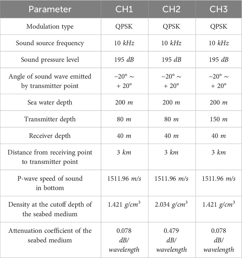
Table 1 Bellhop simulation parameters setup.

Figure 4

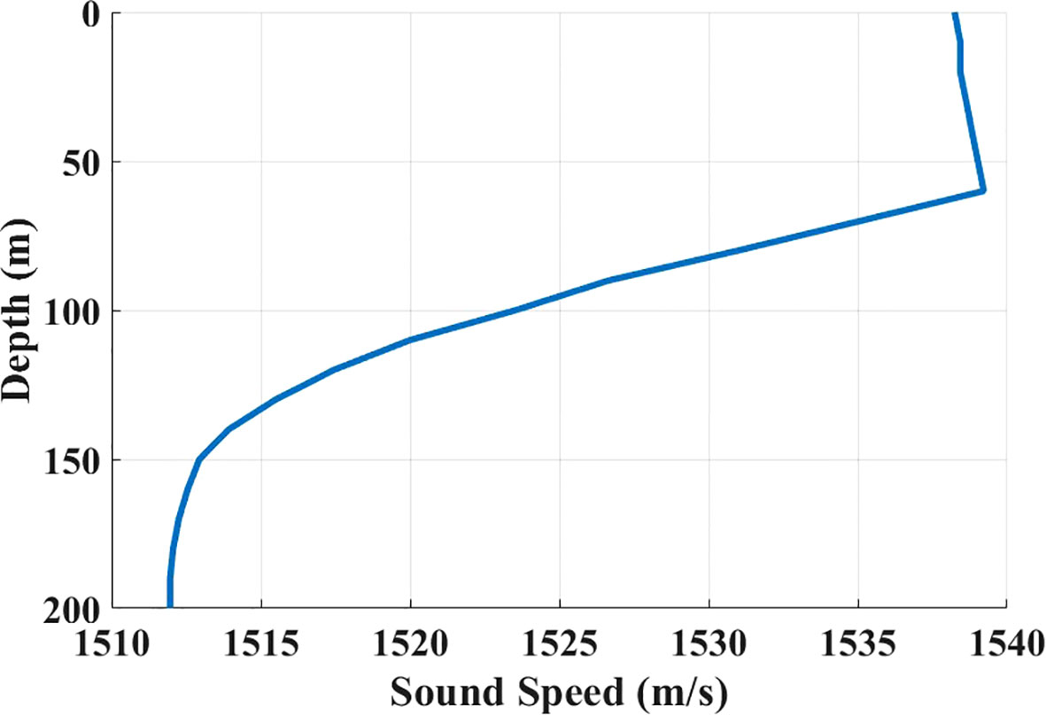
Figure 4 The sound speed profile of 200 m.

Figure 5

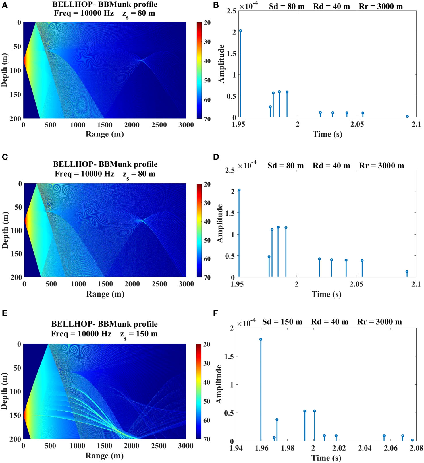
Figure 5 The channel information. (A) The transmission loss at CH1. (B) the impulse response at CH1. (C) The transmission loss at CH2. (D) the impulse response at CH2. (E) The transmission loss at CH3. (F) the impulse response at CH3.

Algorithm 1

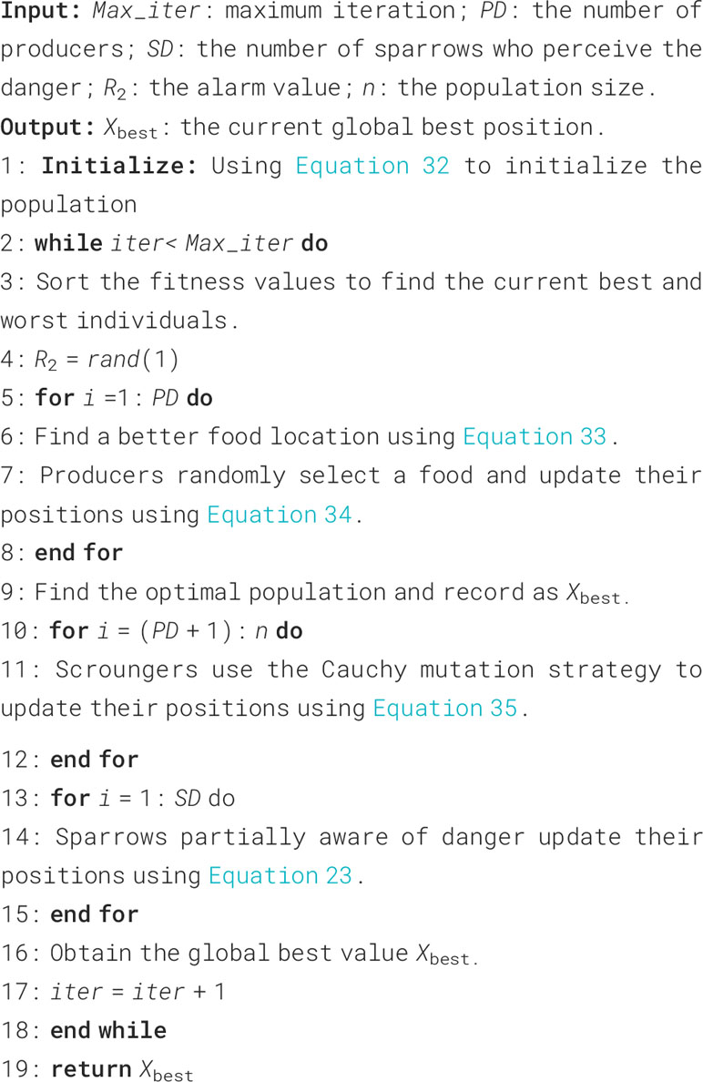
Algorithm 1 The pseudocode of OCCSSA

We will compare equalizers based on MLP (Gibson et al., 1989), CFLNN (Patra et al., 2005), DFCFLNN (Zhao and Zhang, 2008)and traditional DFE with phase-locked loop (PLL) (Stojanovic et al., 1994).

CFLNN has 10 feedforward taps, and its input signal is represented as X_k= [r_k,i,r_k,q,r_k+1,i,r_k+1,q,…, r_k+9,i,r_k+9,q]^T. Here, r_k,irepresents the I-path of the k-th signal, and r_k,q represents the Qpath of the k-th signal. The input signal is transformed into 121 dimensions through a six-order Chebyshev transformation. Therefore, the input layer has 121 nodes, and the output layer has 2 nodes. In DF-CFLNN, the tap coefficient of feedback is 2, and the input signal consists of X_k= [r_k,i,r_k,q,r_k+1,i,r_k+1,q,…,r_k+9,i,r_k+9,q]^T and the feedback signal S_k= [s_k,i,s_k,q,s_k−1, _i,sk−1,q] from the decision device. The input signal is transformed into 97 dimensions through a four order Chebyshev transformation. Therefore, the input layer has 97 nodes, and the output layer has 2 nodes. In SDF-CFLNN, the tap coefficient of feedback is 2, and the input signal X_k=[r_k,i,r_k,q,r_k+1,i,r_k+1,q,…,r_k+9,i,r_k+9,q]^T is transformed into 41 dimensions through a two-order Chebyshev transformation. The input layer has 45 nodes, including 41 nodes for input signals and 4 nodes for feedback signals. The parameters for each equalizer are as shown in Table 2.

Table 2

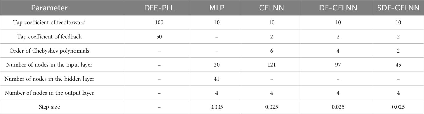
Table 2 Network parameter configuration.

To enhance the reliability, we conducted 30 independent trials on each equalizer. In our setup, we use 10,000 QPSK signals as input data, with 80% serving as training data and 20% as testing data. In each trial, the maximum iteration count was set to 1000. Since this paper focuses on the learning and equalization capabilities of neural networks, in our simulations, we assumed perfect time sequence recovery.

The simulated BER graph is shown in the Figures 6A, C, E. It can be observed that our proposed SDFCFLNNE exhibits the best BER performance in two different underwater acoustic environments, followed by DF-CFLNNE, traditional DFE-PLL, and CFLNNE in descending order. In complex underwater environments, the MLP equalizer performs poorly and is the least effective. The MSE iteration curve at SNR=10 dB is shown in the Figures 6B, D, F. SDF-CFLNNE converges the fastest, with minimal initial oscillations, and exhibits smooth and stable convergence. It also has the smallest MSE value when reaching a steady state. In CH1, SDF-CFLNNE reaches convergence in about 20 iterations, while DFCFLNNE and CFLNNE reach convergence around 300 iterations with minor oscillations. MLP achieves basic convergence in approximately 70 iterations but experiences significant oscillations. In CH2, SDFCFLNNE reaches convergence in about 40 iterations, while DF-CFLNNE, CFLNNE, and MLP all converge around 300 iterations with minor oscillations.

Figure 6

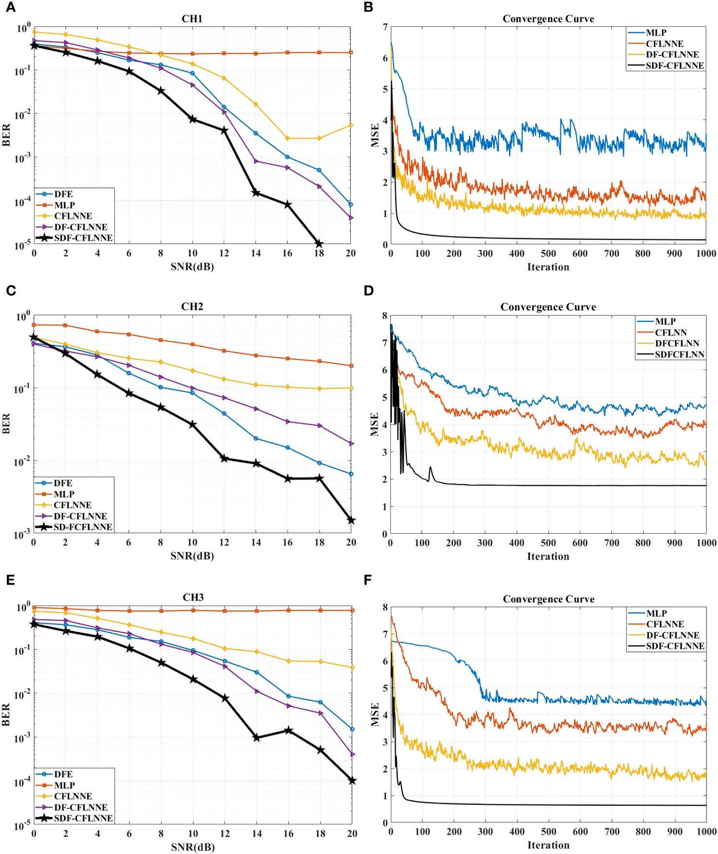
Figure 6 The comparison of the four CFLNN-based and DFE-PLL-based equalizers for CH1, CH2 and CH3. (A) The BER performance for CH1. (B) The MSE performance for CH1 at SNR=10 dB. (C) The BER performance for CH2. (D) The MSE performance for CH2 at SNR=10 dB. (E) The BER performance for CH3. (F) The MSE performance for CH3 at SNR=10 dB.

4.1.2 Comparison of the swarm intelligence optimization algorithms

4.1.2.1 Benchmark test functions

Benchmark test functions are typically utilized to evaluate the performance of optimization algorithms. We utilized the CEC2005 benchmark test functions as provided in Table 3 (Suganthan et al., 2005) to assess the applicability and effectiveness of the proposed OCSSA algorithm.

Table 3

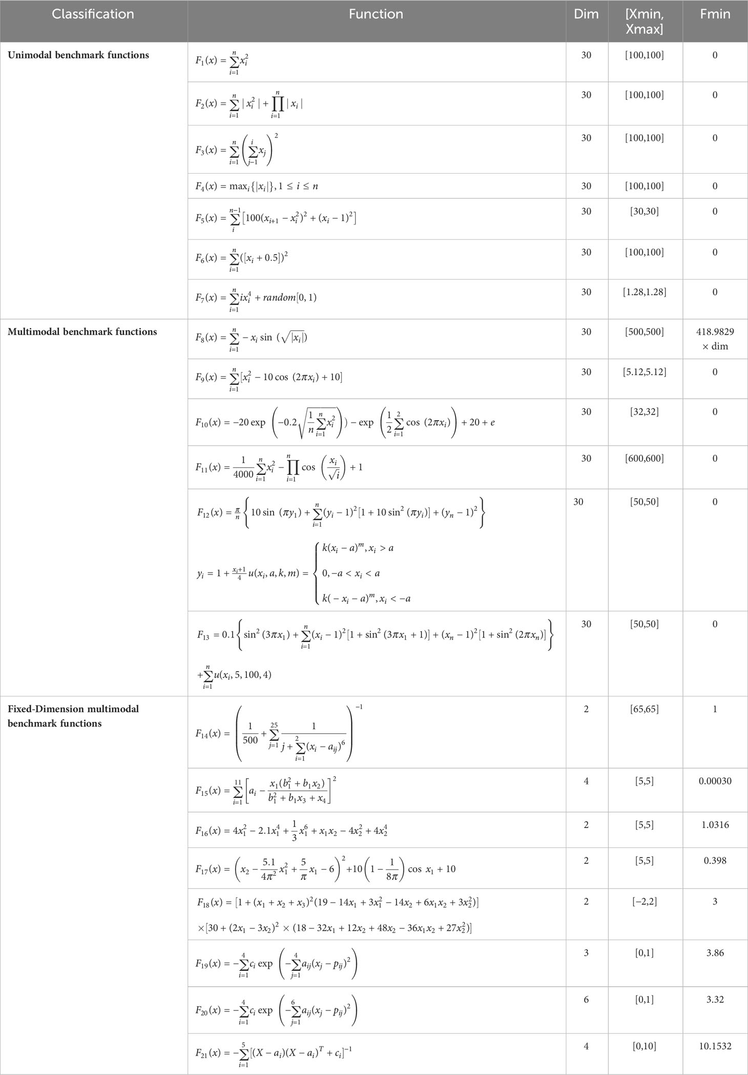
Table 3 Details of the CEC2005 benchmark suite.

4.1.2.2 Comparison of chaotic mapping methods

In order to select the more effective chaotic mapping, we initialized the population of OCCSSA using ten different chaotic mappings, namely Tent, Logistic, Cubic, Chebyshev, Piecewise, Sinusoidal, Sine, ICMIC, Circle, and Bernoulli.

The experimental test environment is as follows: 12th Gen Intel(R) Core(TM) i7-12700H CPU with a base frequency of 2.70 GHz and 16.0 GB of RAM. The operating system used is Windows 11, and the integrated development environment (IDE) is Matlab 2021a.

To increase the credibility of the algorithm, we conducted 30 independent trials on each test function. The maximum iteration count was set to 500, and the population size was 50. The experimental results indicate that overall, the Piecewise chaotic mapping exhibited superior convergence speed and accuracy. We selected the results for F15 and F21, where the convergence effects are more pronounced, for illustration, as shown in Figure 7. Therefore, we chose the Piecewise mapping as the method for random population initialization. The expression for the Piecewise mapping is as shown in Equation 36.

Figure 7

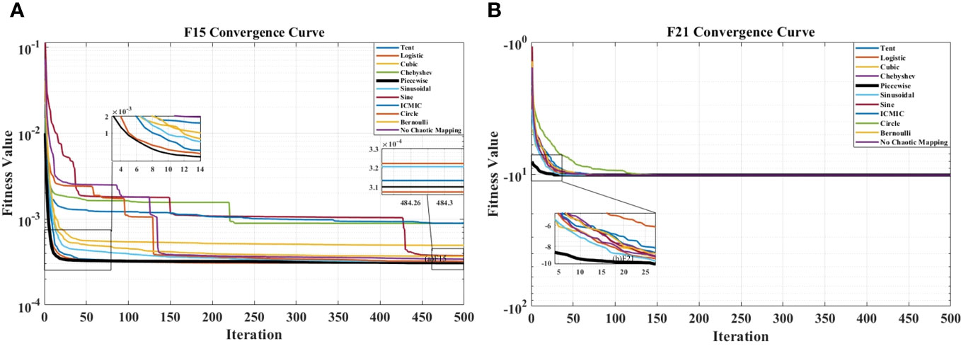
Figure 7 The convergence curves of initializing the OCCSSA population with ten different chaotic mappings: (A) F15. (B) F21.

$\begin{array}{ll}x(t+1)=\{\begin{array}{cc}\frac{x(t)}{p}& ,0\le x(t)<p\\ \frac{x(t)-p}{0.5-p}& ,p\le x(t)<0.5\\ \frac{1-p-x(t)}{0.5-p},0.5\le x(t)<1-p& \\ \frac{1-x(t)}{p},1-p\le x(t)<1& \end{array}& (36)\end{array}$

where $p=0.4,x(1)=rand$.

4.1.2.3 Comparison with the improved SSA-type optimization algorithms

Precision and convergence speed are important indicators for measuring the quality of an algorithm. In order to better validate the effectiveness of the proposed algorithm, this section assesses performance metrics, including convergence precision, using CEC2005 benchmark test functions. This section reproduces SSA (Xue and Shen, 2020), ISSA (Song et al., 2020), and the Adaptive Spiral Flying Sparrow Search Algorithm (ASFSSA) (Ouyang et al., 2021) to compare their performance against the proposed optimization algorithm.

To enhance the algorithm’s reliability, we conducted 30 independent trials on each test function. In each trial, the maximum iteration count was set to 500, and the population size was 50. The safety threshold was set to 0.8, and the number of producers and sparrows sensing danger was both set to 20% of the population size. Tables 4–6 provide the optimization indicators for each algorithm during the optimization process, including the average objective function value, standard deviation, median, best value, average runtime, and algorithm ranking. Under the same standard test functions, the average represents the convergence accuracy of the algorithm, while the standard deviation reflects its stability. The algorithm ranking in this paper is based on both the average and standard deviation, where smaller values indicate better algorithm performance and higher rankings. In cases where the average and standard deviation are the same, the comparison is based on the convergence speed in the convergence curves. When the convergence speeds are similar, the average runtime is considered. The optimal values, algorithms with a ranking of 1, and the shortest average running time among all compared algorithms are highlighted in bold.

Table 4

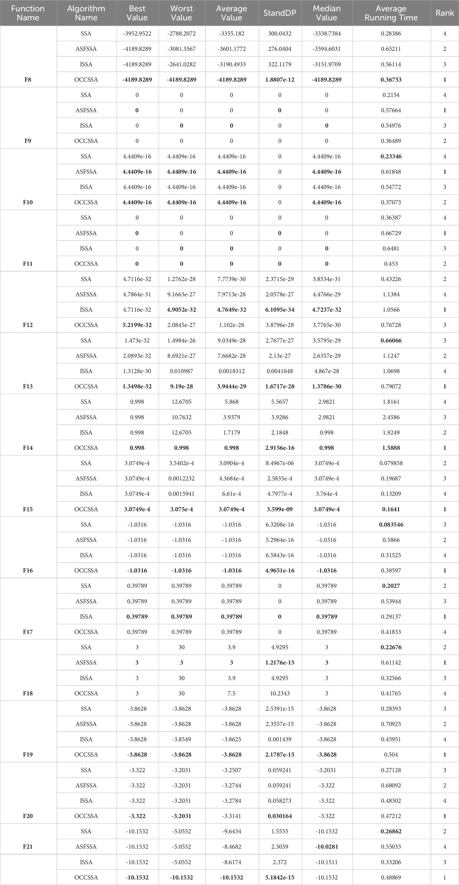
Table 4 The comparative data for the improved SSA-type optimization algorithms on the CEC2005 multi-modal functions.

Table 5

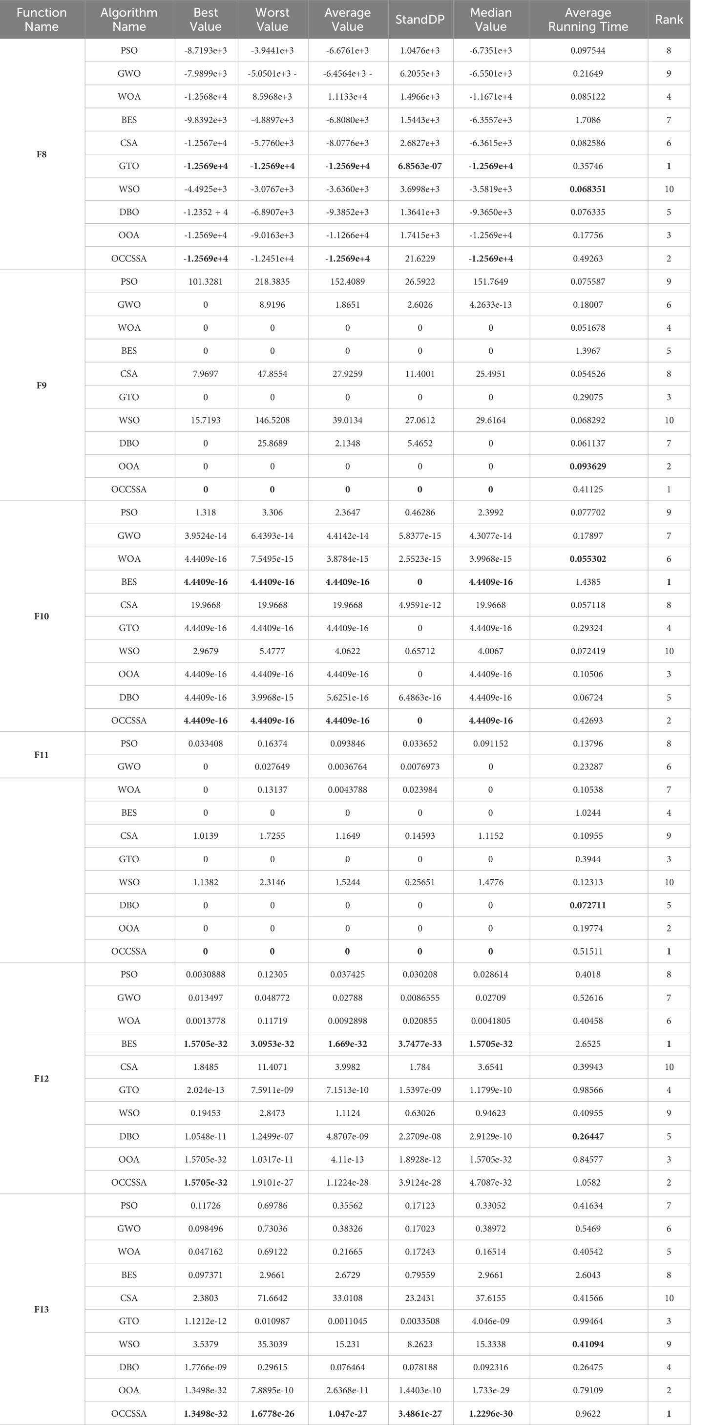
Table 5 The comparative data for the swarm intelligence optimization algorithms on the CEC2005 multimodal functions.

Table 6

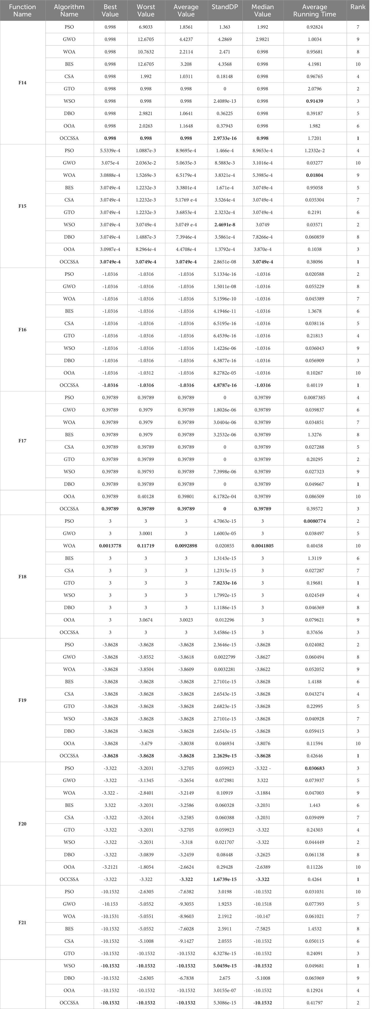
Table 6 The comparative data for the swarm intelligence optimization algorithms on the CEC2005 fixed dimension multi-modal functions.

The data results for the CEC2005 tests are presented in Table 4. Since the optimization of neural network weights involves multi-modal functions, we utilized the second-class functions (F8-F13) and third-class functions (F14-F21) from the CEC2005 benchmark test functions. In the case of CEC2005 multi-modal functions, despite these functions having multiple local optima, the proposed algorithm was able to successfully solve the optimization problems. OCCSSA demonstrated the overall best performance, especially in F8, F13-F15, and F19-F21, where it achieved the best values for each indicator, ranking first. For F9-F11, ASFSSA performed the best, with OCCSSA ranking second. The runtime falls within a moderate range. From the convergence curve plots in Figure 8, it is evident that OCCSSA exhibited superior convergence speed and accuracy in F8, F14-F17, and F19-F21 compared to other algorithms. However, in the case of F18, OCCSSA performed poorly, with lower convergence accuracy than other algorithms. Overall, OCCSSA demonstrated good convergence speed and accuracy, as well as strong resistance to local optima in multi-modal functions. The introduction of multiple strategies significantly improved the algorithm’s stability and search capabilities.

Figure 8

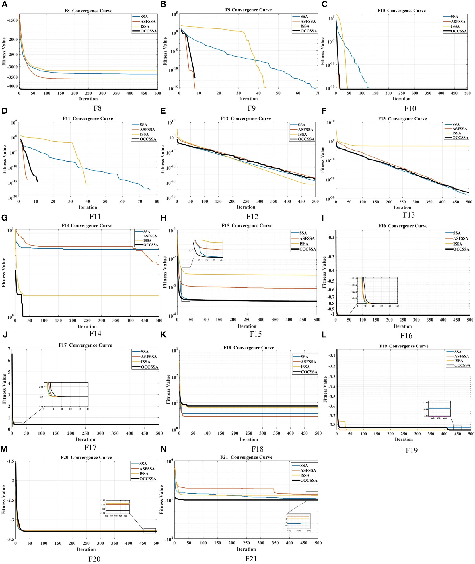
Figure 8 The convergence curve comparison graph of the improved SSA-type optimization algorithms on CEC2005 Multi-Modal functions: (A) F8. (B) F9. (C) F10. (D) F11. (E) F12. (F) F13. (G) F14. (H) F15. (I) F16. (J) F17. (K) F18. (L) F19. (M) F20. (N) F21.

4.1.2.4 Comparison with other swarm intelligence optimization algorithms

To further validate the effectiveness of the proposed algorithm, we compared OCCSSA with other recent swarm intelligence optimization algorithms. These include PSO (Kennedy and Eberhart, 1995), GWO (Mirjalili et al., 2014), WOA (Mirjalili and Lewis, 2016), BES (Alsattar et al., 2020), CSA (Feng et al., 2021), GTO (Abdollahzadeh et al., 2021), DBO (Braik et al., 2022), WSO (Xue and Shen, 2023), and OOA (Dehghani and Trojovskỳ, 2023).

To enhance the credibility of the algorithm, we conducted 30 independent trials on each test function. In each trial, the maximum iteration count was set to 500, and the population size was 50.

The data results for CEC2005 tests are presented in Tables 5, 6. In CEC2005 multi-modal functions, despite the presence of multiple local optima, the proposed algorithm was able to successfully solve the optimization problems. OCCSSA demonstrated the best overall performance, especially in F8-F11, F13-F16, and F20, where it achieved the best values for each indicator, ranking first. For F12 and F21, OCCSSA ranked second, just behind BES and WSO, respectively. In the case of F17 and F18, OCCSSA ranked third. Due to its higher algorithm complexity, the runtime was in the middle to lower range. From the convergence curve plots in Figure 9, it is evident that OCCSSA exhibited overall better convergence speed and accuracy compared to other algorithms. Overall, OCCSSA displayed strong resistance to local optima in multi-modal functions, and the introduction of multiple strategies significantly improved the algorithm’s stability and search capabilities, with good convergence speed and accuracy.

Figure 9

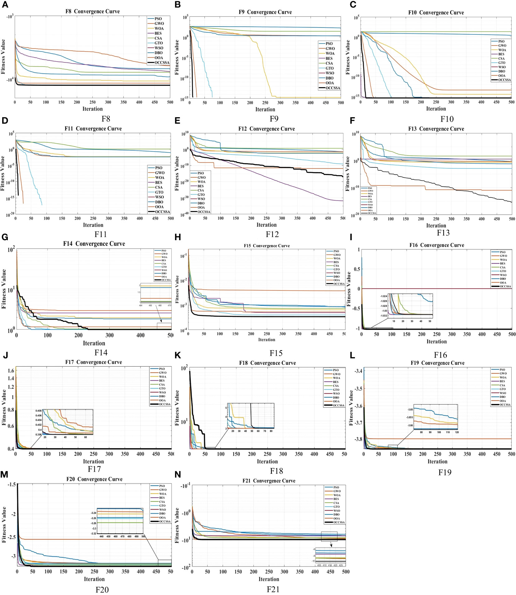
Figure 9 The convergence curve comparison graph of the swarm intelligence optimization algorithms on CEC2005 Multi-Modal functions: (A) F8. (B) F9. (C) F10. (D) F11. (E) F12. (F) F13. (G) F14. (H) F15. (I) F16. (J) F17. (K) F18. (L) F19. (M) F20. (N) F21.

4.1.3 Comparison of the random initialization and OCCSSA initialization of SDF-CFLNNE

During the training phase of a neural network, random initialization of weights and biases can significantly impact the training process and the final performance of the network. To address the issues related to improper initialization, such as gradient vanishing or exploding, and infeasible or slow convergence of the training process, the SDF-CFLNNE initialized intelligently with OCCSSA is proposed. The flowchart is as shown in the Figure 10.

Figure 10

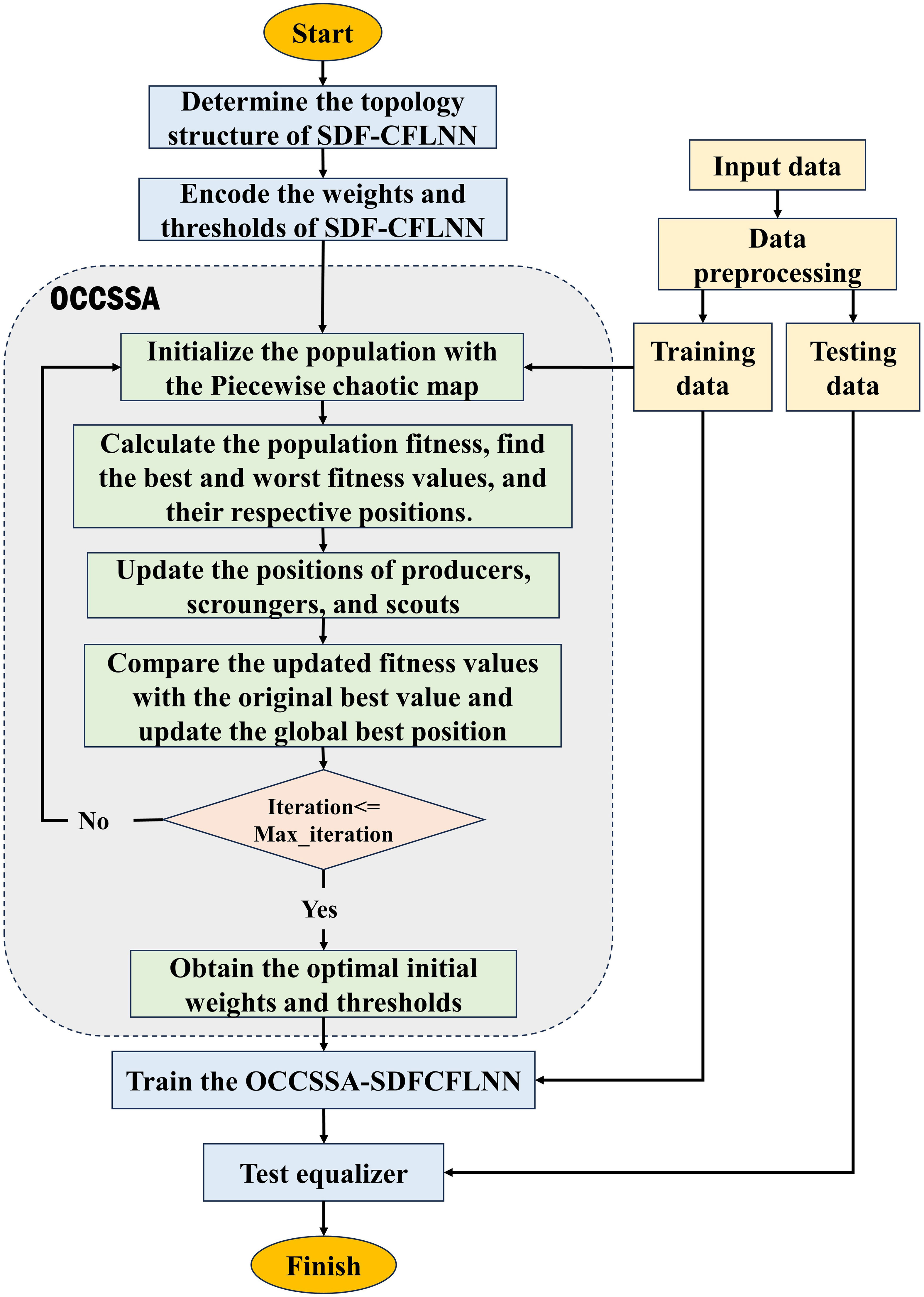
Figure 10 The flowchart of the OCCSSA-SDFCFLNNE.

First, determine the topology of SDF-CFLNN and encode its weights and thresholds. Then, input the encoded population into OCCSSA for initialization using the Piecewise chaotic map. Next, calculate the fitness of the initial population and identify the best and worst population members. OCCSSA updates the positions of producers, scroungers, and scouts. The updated fitness is compared to the original best value, and the global best position is updated. When the maximum iteration is reached, obtain the best population as the initial weights and thresholds for training and testing the network.

We compared the SDFCFLNN equalizers with random initialization (R-SDFCFLNNE) and OCCSSA initialization (OCCSSA-SDFCFLNNE) in both CH1 and CH2 channel environments. To enhance the reliability of the algorithm, we conducted 10 independent experiments. In each experiment, the maximum iteration limit was set to 200, and SDF-CFLNNE still used the parameters from Table 2. For OCCSSA, we used a population size of 50, a safety threshold of 0.8, and the number of producers and the number of sparrows sensing danger were both set to 20% of the population size.

The BER performance of the R-SDFCFLNNE and OCCSSA-SDFCFLNNE are shown in Figures 11A, C, E. OCCSSA-SDFCFLNNE exhibits a slightly lower BER compared to R-SDFCFLNNE. Using CH1 as an example, as observed from Figures 6A, 11A, it is evident that at a BER of 10−³, CFLNNE requires the SNR exceeding 20 dB, DF-CFLNNE requires the SNR of 16 dB, DFE requires the SNR of 13.8 dB, SDF-CFLNNE requires the SNR of 12.8 dB, and OCCSSA-SDFCFLNNE requires the SNR of 12.5 dB. OCCSSA-SDFCFLNNE demonstrates an improvement SNR of 0.2-8 dB compared to CFLNN-based and traditional equalizers. At a BER of 10⁻⁴, CFLNNE requires the SNR exceeding 20 dB, DFE requires the SNR of 19.7 dB, DF-CFLNNE requires the SNR of 18.8 dB, SDF-CFLNNE requires the SNR of 15.5 dB, and OCCSSA-SDFCFLNNE requires the SNR of 13.5 dB. OCCSSA-SDFCFLNNE outperforms CFLNN-based and traditional equalizers, demonstrating an improvement SNR of 2-6 dB.

Figure 11

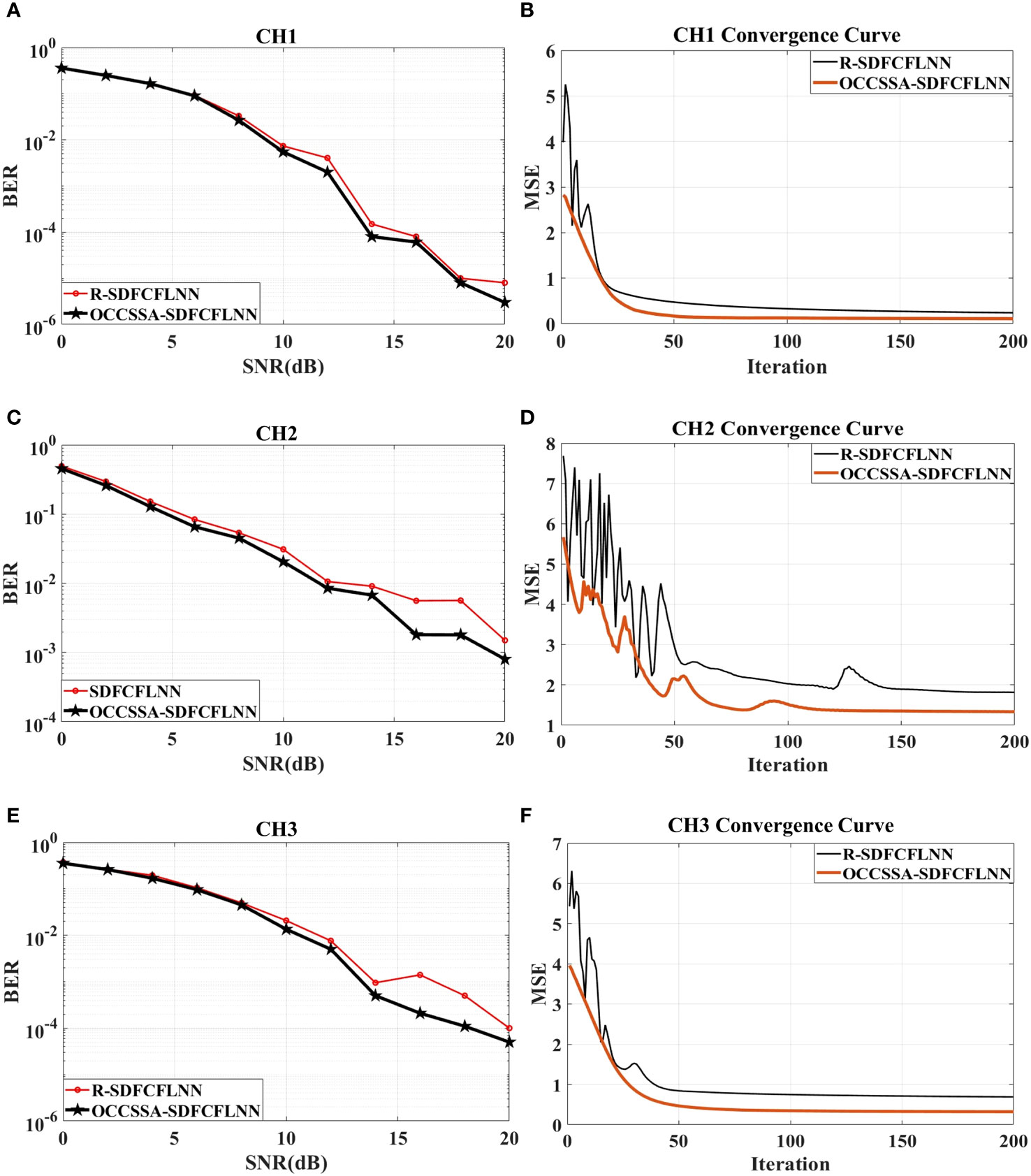
Figure 11 The comparison of the R-SDFCFLNNE and OCCSSA-SDFCFLNNE for CH1, CH2 and CH3. (A) The BER performance for CH1. (B) The MSE performance for CH1 at SNR=10 dB. (C) The BER performance for CH2. (D) The MSE performance for CH2 at SNR=10 dB. (E) The BER performance for CH3. (F) The MSE performance for CH3 at SNR=10 dB.

The MSE performance of the R-SDFCFLNNE and OCCSSA-SDFCFLNNE are shown in Figures 11B, D, F. Both of them converge at almost the same rate. However, R-SDFCFLNNE exhibits minor oscillations in the early iterations, and the curve becomes smooth after convergence. In contrast, OCCSSA-SDFCFLNNE has an extremely smooth convergence curve, which is more stable. The MSE value of OCCSSA-SDFCFLNNE is smaller when it reaches a steady state, indicating more accurate signal recovery. When using OCCSSA initialization, it takes into account the specific characteristics and constraints of the communication channel to provide an optimal set of weight values for network initialization. This can lead to better initial conditions for the network, resulting in improved convergence and signal recovery.

4.2 Lake experiments and results

The analysis of lake experimental data has been presented in this part. On the day of the experiment, there was a slight surface fluctuation on the lake. Before conducting the lake experiments, the hydrophones and other experimental equipment underwent meticulous calibration performed. Additionally, we carried out tasks such as assessing electrical connections and confirming the reliability of communication links within a controlled water tank environment. The equipment connection and layout for the transmitting ship and the receiving ship are as shown in the Figure 12. The distance between the transmitting ship and the receiving ship is either 939m. Both the transmitting and receiving transducers are positioned 10 meters underwater.

Figure 12

Figure 12 The layout diagram of transmitter and receiver.

The system employs QPSK modulation to facilitate data transmission. The signal frame format, as illustrated in Figure 13, has been specifically tailored for complex underwater acoustic conditions. Each data frame incorporates key elements such as Doppler estimation, frame synchronization headers, training sequences, data content, and frame intervals. This frame format is engineered to offer robust anti-Doppler capabilities and effectively mitigate cumulative timing errors. The signal undergoes amplification by a power amplifier and is then transmitted via a transducer. Simultaneously, multiple cycles of underwater acoustic signals are collected by the receivers using a digital collector linked to the transducer. The collected data are processed by DFE-PLL, R-SDFCFLNNE and OCCSSA-SDFCFLNNE. The signal processing flow at the receiving end is depicted in the Figure 14.

Figure 13

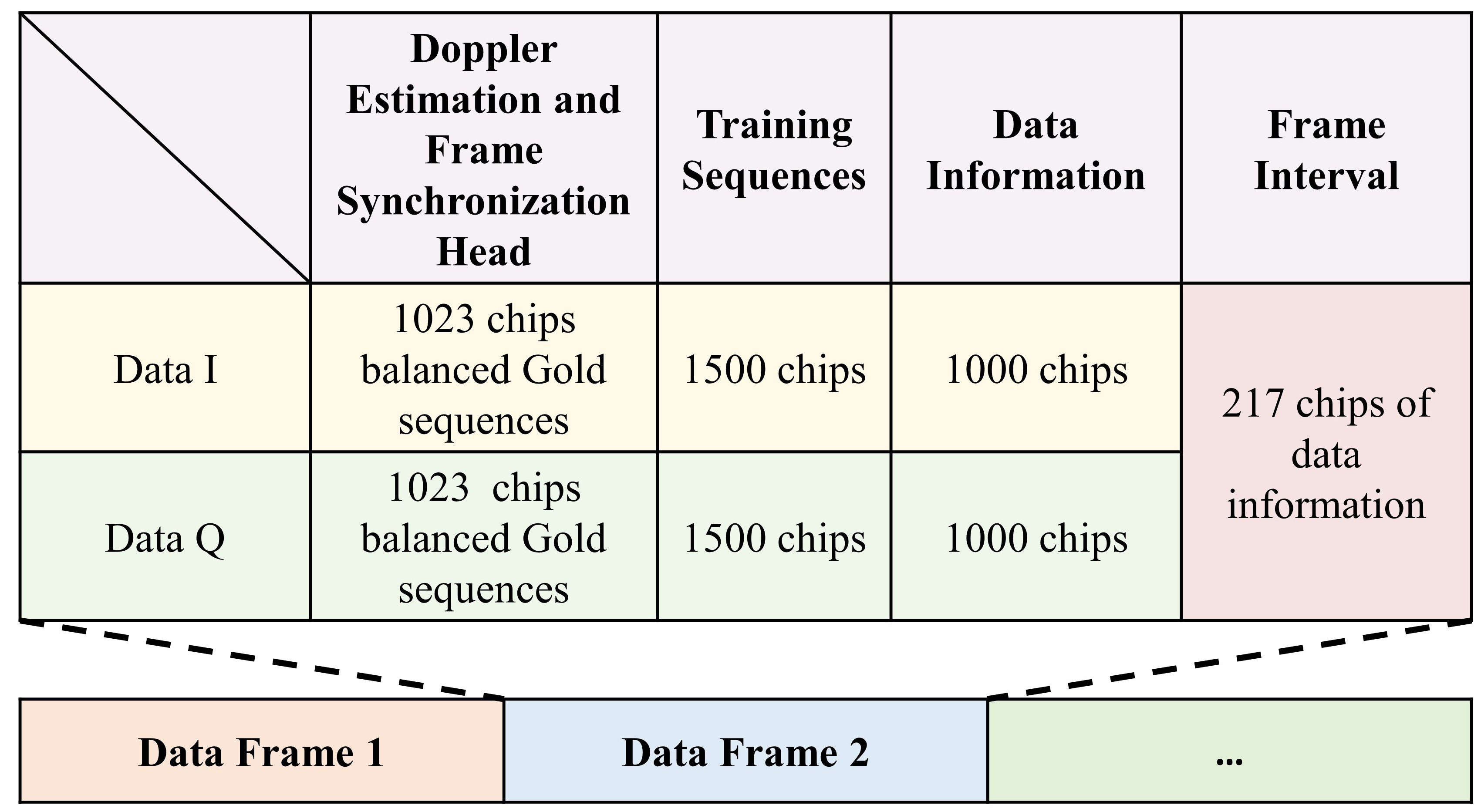
Figure 13 The frame format of the transmitting QPSK signal.

Figure 14

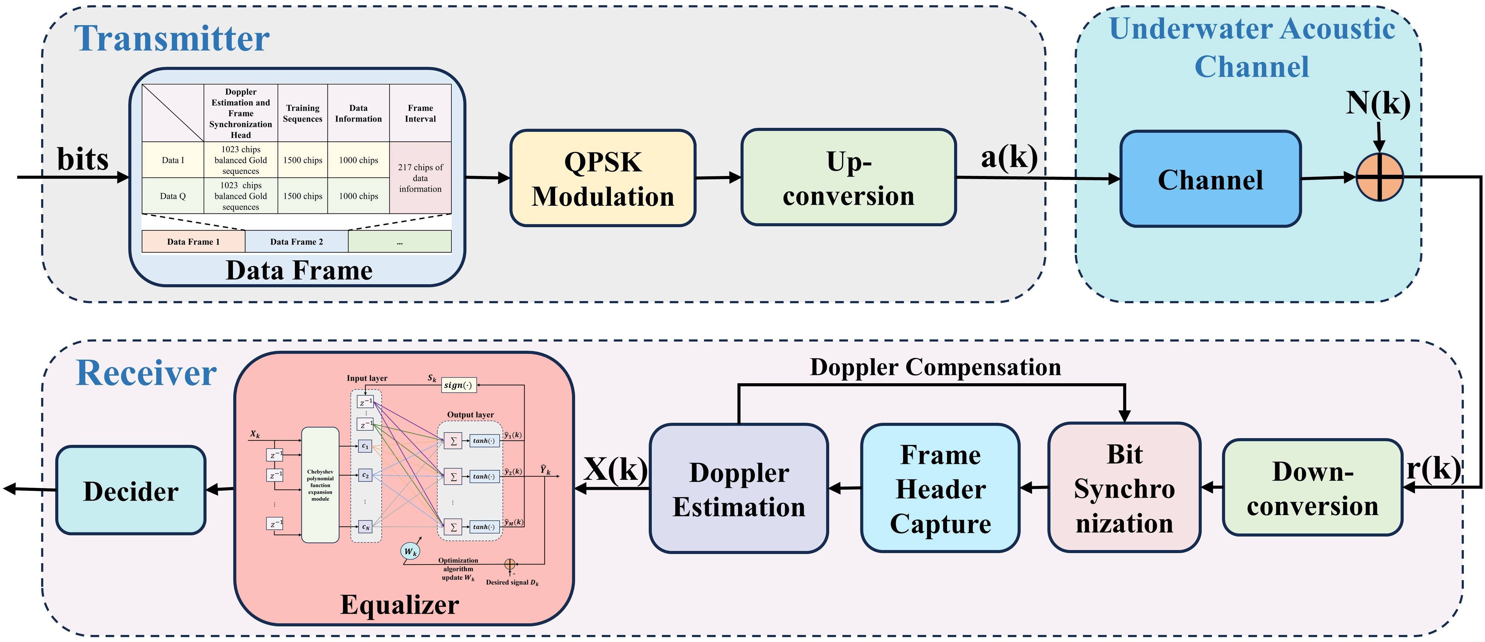
Figure 14 The signal processing flow.

The experimental results are shown in Table 7. We can observe that in the data processing of each frame, OCCSSA-SDFCFLNNE exhibits the lowest BER, followed by R-SDFCFLNNE, and DFE-PLL performing the least favorably. We’ve displayed the MSE convergence curves and the correct and incorrect symbol plots for the second frame of data. Figures 15A, C, E clearly demonstrate that the MSE curve in OCCSSA-SDFCFLNNE converges smoothly and reaches the lowest value, indicating a superior resistance to interference. While R-SDFCFLNNE exhibits minor initial fluctuations, DFE-PLL’s MSE values fluctuate significantly during the initial phase. In Figures 15B, D, F, where blue represents correctly demodulated symbols and red represents incorrectly demodulated symbols, it’s evident that OCCSSA-SDFCFLNNE has the fewest incorrect symbols and the best overall performance.

Table 7

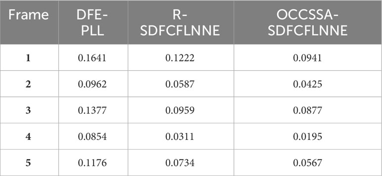
Table 7 The BER comparison of every frame.

Figure 15

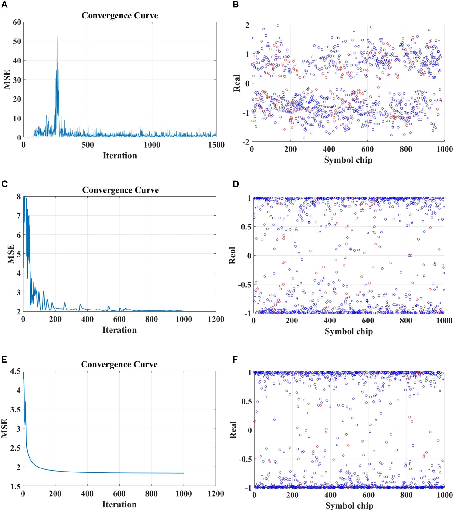
Figure 15 The lake experimental results. (A) The MSE performance for DFE-PLL. (B) The Demodulation correct symbol (blue) and transmission error symbol (red) for DFE-PLL. (C) The MSE performance for R-SDFCFLNNE. (D) The Demodulation correct symbol (blue) and transmission error symbol (red) for R-SDFCFLNNE. (E) The MSE performance for OCCSSA-SDFCFLNNE. (F) The Demodulation correct symbol (blue) and transmission error symbol (red) for OCCSSA-SDFCFLNNE.

5 Conclusion

In the shallow-water environments, underwater communication links are susceptible to significant multipath effects. To address issues such as slow convergence and high system complexity in traditional channel equalizers, this paper proposes a simplified decision feedback Chebyshev function link neural network equalizer (SDF-CFLNNE). The SDF-CFLNNE structure’s innovative approach employs Chebyshev polynomial function expansion modules, eliminating the need for hidden layers and enabling a direct, nonlinear transformation of input signals into the output layer. Additionally, it incorporates the feedback of decision signals into the input layer of the SDF-CFLNN directly, instead of the function expansion module, which significantly reduces computational complexity. However, the effectiveness of neural networks crucially depends on the initial weights and biases, and random initialization can profoundly impact both the training process and the eventual performance of the network. To address this challenge, a novel chaotic sparrow search algorithm combining osprey optimization algorithm and Cauchy mutation (OCCSSA) is proposed. OCCSSA leverages a Piecewise chaotic population initialization strategy, combining the osprey’s exploration tactics with the Cauchy mutation strategy to bolster global and local search capabilities. Simulation experiments, utilizing underwater multipath signals generated by the Bellhop Acoustic Toolbox, unequivocally demonstrate that the SDFCFLNNE initialized by OCCSSA outperforms both CFLNN-based and traditional nonlinear equalizers. Notably, it achieves an impressive 2-6 dB improvement in SNR at a BER of 10⁻⁴ and exhibits a significantly reduced MSE. Furthermore, lake experimental data was employed to validate the effectiveness of the proposed equalizer. These results underscore the remarkable potential of the SDFCFLNNE initialized by OCCSSA as a compelling solution for significantly enhancing the reliability of underwater communication, particularly in the face of the challenges posed by complex underwater environments. This research paves the way for more robust and efficient underwater communication systems, promising increased performance and greater accuracy in signal recovery.

Data availability statement

The original contributions presented in the study are included in the article/supplementary material. Further inquiries can be directed to the corresponding author.

Author contributions

MZ: Conceptualization, Data curation, Methodology, Validation, Writing – original draft, Writing – review & editing. HZ: Funding acquisition, Project administration, Resources, Supervision, Writing – review & editing. TL: Writing – review & editing, Funding acquisition, Project administration, Resources, Supervision. WH: Funding acquisition, Project administration, Resources, Supervision, Writing – review & editing. YD: Writing – review & editing, Data curation, Formal analysis, Investigation. YG: Data curation, Formal analysis, Investigation, Writing – review & editing.

Funding

The author(s) declare financial support was received for the research, authorship, and/or publication of this article. This work was financially supported by the National Natural Science Foundation of China (Grant No. 91938204 and 62271459), the Marine S and T fund of Shandong Province for Pilot National Laboratory for Marine Science and Technology (Qingdao) (No. 2018SDKJ0210).

Conflict of interest

The authors declare that the research was conducted in the absence of any commercial or financial relationships that could be construed as a potential conflict of interest.

Publisher’s note

All claims expressed in this article are solely those of the authors and do not necessarily represent those of their affiliated organizations, or those of the publisher, the editors and the reviewers. Any product that may be evaluated in this article, or claim that may be made by its manufacturer, is not guaranteed or endorsed by the publisher.

References

Abdollahzadeh B., Soleimanian Gharehchopogh F., Mirjalili S. (2021). Artificial gorilla troops optimizer: a new nature-inspired metaheuristic algorithm for global optimization problems. Int. J. Intelligent Syst. 36, 5887–5958. doi: 10.1002/int.22535

CrossRef Full Text | Google Scholar

Alsattar H. A., Zaidan A., Zaidan B. (2020). Novel meta-heuristic bald eagle search optimisation algorithm. Artif. Intell. Rev. 53, 2237–2264. doi: 10.1007/s10462-019-09732-5

CrossRef Full Text | Google Scholar

Barnard C. J., Sibly R. M. (1981). Producers and scroungers: a general model and its application to captive flocks of house sparrows. Anim. Behav. 29, 543–550. doi: 10.1016/S0003-3472(81)80117-0

CrossRef Full Text | Google Scholar

Braik M., Hammouri A., Atwan J., Al-Betar M. A., Awadallah M. A. (2022). White shark optimizer: A novel bio-inspired meta-heuristic algorithm for global optimization problems. KnowledgeBased Syst. 243, 108457. doi: 10.1016/j.knosys.2022.108457

CrossRef Full Text | Google Scholar

Burse K., Yadav R. N., Shrivastava S. (2010). Channel equalization using neural networks: A review. IEEE Trans. systems man cybernetics Part C (Applications Reviews) 40, 352–357. doi: 10.1109/TSMCC.2009.2038279

CrossRef Full Text | Google Scholar

Chagra W., Bouani F., Abdennour R. B., Ksouri M., Favier G. (2005). Equalization with decision delay estimation using recurrent neural networks. Adv. Eng. Software 36, 442–447. doi: 10.1016/j.advengsoft.2005.01.011

CrossRef Full Text | Google Scholar

Chang Y.-J., Ho C.-L. (2009). “Decision feedback equalizers using self-constructing fuzzy neural networks,” in 2009 Fourth International Conference on Innovative Computing, Information and Control (ICICIC). 1483–1486 (IEEE).

Google Scholar

Chang Y.-J., Ho C.-L. (2011). Scfnn-based decision feedback equalization robust to frequency offset and phase noise. Circuits Systems Signal Process. 30, 929–940. doi: 10.1007/s00034-010-9258-5

CrossRef Full Text | Google Scholar

Chang P.-R., Wang B.-C. (1995). Adaptive decision feedback equalization for digital satellite channels using multilayer neural networks. IEEE J. selected areas Commun. 13, 316–324. doi: 10.1109/49.345876

CrossRef Full Text | Google Scholar

Dehghani M., Trojovskỳ P. (2023). Osprey optimization algorithm: A new bio-inspired metaheuristic algorithm for solving engineering optimization problems. Front. Mechanical Eng. 8, 1126450. doi: 10.3389/fmech.2022.1126450

CrossRef Full Text | Google Scholar

Feng Z.-k., Niu W.-j., Liu S. (2021). Cooperation search algorithm: A novel metaheuristic evolutionary intelligence algorithm for numerical optimization and engineering optimization problems. Appl. Soft Computing 98, 106734. doi: 10.1016/j.asoc.2020.106734

CrossRef Full Text | Google Scholar

Freitag L., Johnson M., Stojanovic M. (1997). “Efficient equalizer update algorithms for acoustic communication channels of varying complexity,” in Oceans’ 97. MTS/IEEE Conference Proceedings (Halifax, NS, Canada: IEEE), Vol. 1. 580–585.

Google Scholar

Gao M., Guo Y.-c., Liu Z.-x., Zhang Y.-p. (2009). “Feed-forward neural network blind equalization algorithm based on super-exponential iterative,” in 2009 International Conference on Intelligent HumanMachine Systems and Cybernetics (Hangzhou, China: IEEE), Vol. 1. 335–338.

Google Scholar

Ge W., Wang Z., Yin J., Han X. (2022). Robust equalization for single-carrier underwater acoustic communications based on parameterized interference model. IEEE Wireless Commun. Lett. doi: 10.1109/LWC.2022.3223533

CrossRef Full Text | Google Scholar

Gibson G. J., Siu S., Cowen C. (1989). “Multilayer perceptron structures applied to adaptive equalisers for data communications,” in International Conference on Acoustics, Speech, and Signal Processing (Glasgow, UK: IEEE), 1183–1186.

Google Scholar

Guha D. R., Patra S. K. (2009). “Isi and burst noise interference minimization using wilcoxon generalized radial basis function equalizer,” in 2009 Fifth International Conference on MEMS NANO, and Smart Systems (Dubai, United Arab Emirates: IEEE), 89–92.

Google Scholar

He C., Jing L., Xi R., Wang H., Hua F., Dang Q., et al. (2019). Time-frequency domain turbo equalization for single-carrier underwater acoustic communications. IEEE Access 7, 73324–73335. doi: 10.1109/ACCESS.2019.2919757

CrossRef Full Text | Google Scholar

He Y., Tao Y. (2023). “Deep reinforcement learning based cognitive equalization algorithm research in underwater communication,” in 2023 IEEE 3rd International Conference on Computer Communication and Artificial Intelligence (CCAI) (Taiyuan, China: IEEE), 348–352.

Google Scholar

He Q., Tao J., Kong X., Zhuang Y., Jiang M., Qiao Y. (2023). “Channel replay aided neural network equalizer for underwater acoustic communications,” in OCEANS 2023-Limerick (Limerick, Ireland: IEEE), 1–5).

Google Scholar

Heng S., Chen W., Yin H., Shiping M., Jizhang Z. (2006). Decision feedback equalizer based on non-singleton fuzzy regular neural networks. J. Syst. Eng. Electron. 17, 896–900. doi: 10.1016/S1004-4132(07)60034-6

CrossRef Full Text | Google Scholar

Huang J.-g., Wang H., He C.-b., Zhang Q.-f., Jing L.-y. (2018). Underwater acoustic communication and the general performance evaluation criteria. Front. Inf. Technol. Electronic Eng. 19, 951–971. doi: 10.1631/FITEE.1700775

CrossRef Full Text | Google Scholar

Hussain A., Soraghan J. J., Durrani T. S. (1997). A new adaptive functional-link neural-networkbased dfe for overcoming co-channel interference. IEEE Trans. Commun. 45, 1358– 1362. doi: 10.1109/26.649741

CrossRef Full Text | Google Scholar

Ingle K. K., Jatoth R. K. (2023). Non-linear channel equalization using modified grasshopper optimization algorithm. Appl. Soft Computing 110091. doi: 10.1016/j.asoc.2023.110091

CrossRef Full Text | Google Scholar

Kari D., Vanli N. D., Kozat S. S. (2017). Adaptive and efficient nonlinear channel equalization for underwater acoustic communication. Phys. Communication 24, 83–93. doi: 10.1016/j.phycom.2017.06.001

PubMed Abstract | CrossRef Full Text | Google Scholar

Kechriotis G., Zervas E., Manolakos E. S. (1994). Using recurrent neural networks for adaptive communication channel equalization. IEEE Trans. Neural Networks 5, 267–278. doi: 10.1109/72.279190

PubMed Abstract | CrossRef Full Text | Google Scholar

Kennedy J., Eberhart R. (1995). “Particle swarm optimization,” in Proceedings of ICNN’95international conference on neural networks (WA, Australia: IEEE), Vol. 4, 1942–1948.

Google Scholar

Lee T.-T., Jeng J.-T. (1998). The chebyshev-polynomials-based unified model neural networks for function approximation. IEEE Trans. Systems Man Cybernetics Part B (Cybernetics) 28, 925–935.

Google Scholar

Lee J., Sankar R. (2007). Theoretical derivation of minimum mean square error of rbf based equalizer. Signal Process. 87, 1613–1625. doi: 10.1016/j.sigpro.2007.01.008

CrossRef Full Text | Google Scholar

Li Y., Geng T., Tian R., Gao S. (2021). Machine-learning based equalizers for mitigating the interference in asynchronous mimo owc systems. J. Lightwave Technol. 39, 2800–2808. doi: 10.1109/JLT.2021.3057396

PubMed Abstract | CrossRef Full Text | Google Scholar

Liker A., Barta Z. (2002). The effects of dominance on social foraging tactic use in house sparrows. Behaviour, 1061–1076. doi: 10.1163/15685390260337903

CrossRef Full Text | Google Scholar

Liu W., Liu J., Liu T., Chen H., Wang Y.-L. (2023). Detector design and performance analysis for target detection in subspace interference. IEEE Signal Process. Lett. doi: 10.1109/LSP.2023.3270080

PubMed Abstract | CrossRef Full Text | Google Scholar

Liu J., Mei K., Zhang X., Ma D., Wei J. (2019). Online extreme learning machine-based channel estimation and equalization for ofdm systems. IEEE Commun. Lett. 23, 1276–1279. doi: 10.1109/LCOMM.2019.2916797

PubMed Abstract | CrossRef Full Text | Google Scholar

Ma X., Ye H., Li Y. (2018). “Learning assisted estimation for time-varying channels,” in 2018 15th international symposium on wireless communication systems (ISWCS) (Lisbon, Portugal: IEEE), 1–5.

Google Scholar

Milan A., Rezatofighi S. H., Dick A., Reid I., Schindler K. (2017). “Online multi-target tracking using recurrent neural networks,” in Proceedings of the AAAI conference on Artificial Intelligence, Vol. 31.

Google Scholar

Mirjalili S., Lewis A. (2016). The whale optimization algorithm. Adv. Eng. software 95, 51–67. doi: 10.1016/j.advengsoft.2016.01.008

PubMed Abstract | CrossRef Full Text | Google Scholar

Mirjalili S., Mirjalili S. M., Lewis A. (2014). Grey wolf optimizer. Adv. Eng. software 69, 46–61. doi: 10.1016/j.advengsoft.2013.12.007

CrossRef Full Text | Google Scholar

Mishra J. P., Singh K., Chaudhary H. (2023). “Recent advancement of ai technology for underwater acoustic communication,” in AIP Conference Proceedings (AIP Publishing). (Jaipur, India: IEEE), Vol. 2752.

Google Scholar

Mohapatra P. K., Rout S. K., Bisoy S. K., Sain M. (2022). Training strategy of fuzzy-firefly based ann in non-linear channel equalization. IEEE Access 10, 51229–51241. doi: 10.1109/ACCESS.2022.3174369

CrossRef Full Text | Google Scholar

Ning X., Liu Z., Luo Y. (2009). “Research on variable step-size blind equalization algorithm based on normalized rbf neural network in underwater acoustic communication,” in Advances in Neural Networks–ISNN 2009: 6th International Symposium on Neural Networks, ISNN 2009 Wuhan, China, May 26-29, 2009 Proceedings, Part III 6 (Berlin Heidelberg: Springer), 1063–1070.

Google Scholar

Ouyang C., Qiu Y., Zhu D. (2021). Adaptive spiral flying sparrow search algorithm. Sci. Programming 2021, 1–16. doi: 10.1155/2021/6505253

CrossRef Full Text | Google Scholar

Patra J. C., Chin W. C., Meher P. K., Chakraborty G. (2008). “Legendre-flann-based nonlinear channel equalization in wireless communication system,” in 2008 IEEE international conference on systems, man and cybernetics (Singapore: IEEE), 1826–1831.

Google Scholar

Patra J. C., Kot A. C. (2002). Nonlinear dynamic system identification using chebyshev functional link artificial neural networks. IEEE Trans. Systems Man Cybernetics Part B (Cybernetics) 32, 505–511. doi: 10.1109/TSMCB.2002.1018769

CrossRef Full Text | Google Scholar

Patra J. C., Pal R. N., Baliarsingh R., Panda G. (1999). Nonlinear channel equalization for qam signal constellation using artificial neural networks. IEEE Trans. Systems Man Cybernetics Part B (Cybernetics) 29, 262–271. doi: 10.1109/3477.752798

CrossRef Full Text | Google Scholar

Patra J. C., Poh W. B., Chaudhari N. S., Das A. (2005). “Nonlinear channel equalization with qam signal using chebyshev artificial neural network,” in Proceedings. 2005 IEEE International Joint Conference on Neural Networks, 2005 (Montreal, QC, Canada: IEEE), Vol. 5. 3214–3219.

Google Scholar

Qiao G., Liu Y., Zhou F., Zhao Y., Mazhar S., Yang G. (2022). Deep learning-based m-ary spread spectrum communication system in shallow water acoustic channel. Appl. Acoustics 192, 108742. doi: 10.1016/j.apacoust.2022.108742

CrossRef Full Text | Google Scholar

Qin X., Qu F., Zheng Y. R. (2020). Bayesian iterative channel estimation and turbo equalization for multiple-input–multiple-output underwater acoustic communications. IEEE J. Oceanic Eng. 46, 326–337. doi: 10.1109/JOE.2019.2956299

CrossRef Full Text | Google Scholar

Sahu J., Majumder S. (2021). “A particle swarm optimization based training algorithm for mcma blind adaptive equalizer,” in 2021 International Conference on Emerging Smart Computing and Informatics (ESCI) (Pune, India: IEEE), 462–465.

Google Scholar

Shwetha N., Priyatham M., Gangadhar N. (2023). Artificial neural network based channel equalization using battle royale optimization algorithm with different initialization strategies. Multimedia Tools Appl. 1–26. doi: 10.1007/s11042-023-16161-8

CrossRef Full Text | Google Scholar

Song H. C., Hodgkiss W., Kuperman W., Stevenson M., Akal T. (2006). Improvement of timereversal communications using adaptive channel equalizers. IEEE J. Oceanic Eng. 31, 487–496. doi: 10.1109/JOE.2006.876139

CrossRef Full Text | Google Scholar

Song W., Liu S., Wang X., Wu W. (2020). “An improved sparrow search algorithm,” in 2020 IEEE Intl Conf on Parallel & Distributed Processing with Applications, Big Data & Cloud Computing, Sustainable Computing & Communications, Social Computing & Networking (ISPA/BDCloud/SocialCom/SustainCom). 537–543 (IEEE).

Google Scholar

Stojanovic M., Catipovic J. A., Proakis J. G. (1994). Phase-coherent digital communications for underwater acoustic channels. IEEE J. oceanic Eng. 19, 100–111. doi: 10.1109/48.289455

CrossRef Full Text | Google Scholar

Stojanovic M., Preisig J. (2009). Underwater acoustic communication channels: Propagation models and statistical characterization. IEEE Commun. magazine 47, 84–89. doi: 10.1109/MCOM.2009.4752682

CrossRef Full Text | Google Scholar

Suganthan P. N., Hansen N., Liang J. J., Deb K., Chen Y.-P., Auger A., et al. (2005). Problem definitions and evaluation criteria for the cec 2005 special session on real-parameter optimization. KanGAL Rep. 2005005 2005.

Google Scholar

Tsai C.-W., Lai C.-F., Chiang M.-C., Yang L. T. (2013). Data mining for internet of things: A survey. IEEE Commun. Surveys Tutorials 16, 77–97. doi: 10.1109/SURV.2013.103013.00206

CrossRef Full Text | Google Scholar

van Heteren M. (2022). Link adaptation and equalization for underwater acoustic communication using machine learning.

Google Scholar

Wang Z., Chen F., Yu H., Shan Z. (2021). Sparse decision feedback equalization for underwater acoustic channel based on minimum symbol error rate. Int. J. Naval Architecture Ocean Eng. 13, 617–627. doi: 10.1016/j.ijnaoe.2021.07.004

CrossRef Full Text | Google Scholar

Wang T., Wen C.-K., Wang H., Gao F., Jiang T., Jin S. (2017). Deep learning for wireless physical layer: Opportunities and challenges. China Commun. 14, 92–111. doi: 10.1109/CC.2017.8233654

CrossRef Full Text | Google Scholar

Wei G., Yizhen J., Xiao H., Xiao Z., Wentao T. (2023). Robust equalization for single-carrier underwater acoustic communication in sparse impulsive interference environment. Appl. Acoustics 214, 109706. doi: 10.1016/j.apacoust.2023.109706

CrossRef Full Text | Google Scholar

Xi J., Yan S., Xu L., Hou C. (2020). Sparsity-aware adaptive turbo equalization for underwater acoustic communications in the mariana trench. IEEE J. Oceanic Eng. 46, 338–351. doi: 10.1109/JOE.2020.2982808

CrossRef Full Text | Google Scholar

Xi J., Yan S., Xu L., Zhang Z., Zeng D. (2019). Frequency–time domain turbo equalization for underwater acoustic communications. IEEE J. Oceanic Eng. 45, 665–679. doi: 10.1109/JOE.2019.2891171

CrossRef Full Text | Google Scholar

Xiao Y., Dong Y. (2015). Instantaneous gradient based dual mode wavelet neural network blind equalization for underwater acoustic channel. Appl. Mathematics Inf. Sci. 9, 1467. doi: 10.12785/amis/090341

CrossRef Full Text | Google Scholar

Xiao Y., Dong Y., Li Z. (2008). “Blind equalization in underwater acoustic communication by recurrent neural network with bias unit,” in 2008 7th World Congress on Intelligent Control and Automation (Chongqing, China: IEEE), 2407–2410.

Google Scholar

Xue J., Shen B. (2020). A novel swarm intelligence optimization approach: sparrow search algorithm. Syst. Sci. control Eng. 8, 22–34. doi: 10.1080/21642583.2019.1708830

CrossRef Full Text | Google Scholar

Xue J., Shen B. (2023). Dung beetle optimizer: A new meta-heuristic algorithm for global optimization. J. Supercomputing 79, 7305–7336. doi: 10.1007/s11227-022-04959-6

CrossRef Full Text | Google Scholar

Yang R., Yang L., Zhang J., Sun C., Cong W., Zhu S. (2018). “Blind equalization of qam signals via extreme learning machine,” in 2018 Tenth International Conference on Advanced Computational Intelligence (ICACI) (Xiamen, China: IEEE), 34–39.

Google Scholar

Zhang Y., Li C., Wang H., Wang J., Yang F., Meriaudeau F. (2022). Deep learning aided ofdm receiver for underwater acoustic communications. Appl. Acoustics 187, 108515. doi: 10.1016/j.apacoust.2021.108515

CrossRef Full Text | Google Scholar

Zhang Y., Li J., Zakharov Y. V., Li J., Li Y., Lin C., et al. (2019b). Deep learning based single carrier communications over time-varying underwater acoustic channel. IEEE Access 7, 38420–38430. doi: 10.1109/ACCESS.2019.2906424

CrossRef Full Text | Google Scholar

Zhang X.-L., Wang D. (2016). A deep ensemble learning method for monaural speech separation. IEEE/ACM Trans. audio speech Lang. Process. 24, 967–977. doi: 10.1109/TASLP.2016.2536478

CrossRef Full Text | Google Scholar

Zhang X., Wu H., Sun H., Ying W. (2021). Multireceiver sas imagery based on monostatic conversion. IEEE J. Selected Topics Appl. Earth Observations Remote Sens. 14, 10835–10853. doi: 10.1109/JSTARS.2021.3121405

CrossRef Full Text | Google Scholar

Zhang L., Yang L.-L. (2020). Machine learning for joint channel equalization and signal detection. Mach. Learn. Future Wireless Commun., 213–241. doi: 10.1002/9781119562306.ch12

CrossRef Full Text | Google Scholar

Zhang G., Yang L., Chen L., Zhao B., Li Y., Wei W. (2019a). “Blind equalization algorithm for underwater acoustic channel based on support vector regression,” in 2019 11th International Conference on Intelligent Human-Machine Systems and Cybernetics (IHMSC) (IHMSC) (Hangzhou, China: IEEE), Vol. 2. 163–166.

Google Scholar

Zhang Y., Zakharov Y. V., Li J. (2018). Soft-decision-driven sparse channel estimation and turbo equalization for mimo underwater acoustic communications. IEEE Access 6, 4955–4973. doi: 10.1109/ACCESS.2018.2794455

CrossRef Full Text | Google Scholar

Zhao H., Zeng X., Zhang J., Li T. (2010). Nonlinear adaptive equalizer using a pipelined decision feedback recurrent neural network in communication systems. IEEE Trans. Commun. 58, 2193–2198. doi: 10.1109/TCOMM.2010.08.080612

CrossRef Full Text | Google Scholar

Zhao H., Zeng X., Zhang X., Zhang J., Liu Y., Wei T. (2011). An adaptive decision feedback equalizer based on the combination of the fir and flnn. Digital Signal Process. 21, 679–689. doi: 10.1016/j.dsp.2011.05.004

CrossRef Full Text | Google Scholar

Zhao H., Zhang J. (2008). Functional link neural network cascaded with chebyshev orthogonal polynomial for nonlinear channel equalization. Signal Process. 88, 1946–1957. doi: 10.1016/j.sigpro.2008.01.029

CrossRef Full Text | Google Scholar

Zhou M., Zhang H., Lv T., Li H., Xiang D., Huang S., et al. (2022). “Underwater acoustic channel modeling under different shallow seabed topography and sediment environment,” in OCEANS 2022Chennai (Chennai, India: IEEE), 1–7.

Google Scholar

Zhu J., Song Y., Jiang N., Xie Z., Fan C., Huang X. (2023). Enhanced doppler resolution and sidelobe suppression performance for golay complementary waveforms. Remote Sens. 15, 2452. doi: 10.3390/rs15092452

CrossRef Full Text | Google Scholar