The two salinity peaks mode of marine salt supply to coastal underground brine during a single tidal cycle

Seawater salt is constantly supplied from the marine environment to coastal underground brine deposits, meaning that brine has the potential for continuous extraction. There is currently a lack of information about the processes that drive the fluxes of seawater salt to underground brine deposits in tidal-driven brine mining areas. We chose the Yangkou salt field on the southern coast of Laizhou Bay, a brine mining area, as our study site. We monitored the spatial and temporal distribution of the underground brine reserve and the changes in water level and salinity in the mining area and adjacent tidal flats using electrical resistivity tomography and hydrogeological measurements. We monitored cross-sections along two survey lines and observed that the underground brine reserve receives a stable supply of seawater salt, and calculated that the rate of influx into the brine body in the mining area near the boundary of the precipitation funnel was 0.226−0.232 t/h. We calculated that a total salt flux of approximately 5.50 t enters the underground brine body every day through a 150 m long shoreline and a 1322.3 m² window, which is sufficient to sustain the daily extraction of one brine well. During tidal cycles, there are two peaks in the salinity of the water supplied to the underground brine reserve, which means that the brine supply is from at least two high-salinity salt sources in different tidal stages. The first salinity peak occurs during the initial stage of the rising tide after seawater inundates the tidal flat. At this time, seawater, which is a solution and carries a large amount of evaporated salt, is transported into the brine layer through highly permeable areas or biological channels and replenishes the brine in the mining area. The second salinity peak occurs during the early stage of the falling tide. Influenced by hysteresis-driven tidal pumping, high-salinity brine from the lower intertidal zone is rapidly transported into the mining area, thereby increasing the salinity of the underground brine.

1 Introduction

Coastal underground brine reserves constitute an important source of minerals for salt production and the extraction of bromine, iodine, and other chemical raw materials. These reserves are generally distributed in bay areas in semi-arid and arid climatic zones between 50° north and south worldwide (Sanford and Wood, 2001; Frank et al., 2009; Zhang, 2021) (Figure 1). The marine environment is the main source of salt for these coastal underground brine resources and, under the combined influence of ocean dynamics (density difference, tides, storm surges, etc.) and evaporation, shallow coastal underground brine reserves in extraction areas receive continuous supplies of water and salt supplies (Han, 1996; Boufadel, 2000; Robinson et al., 2007; Gonneea et al., 2013; Post et al., 2013; Sun et al., 2023).

Figure 1

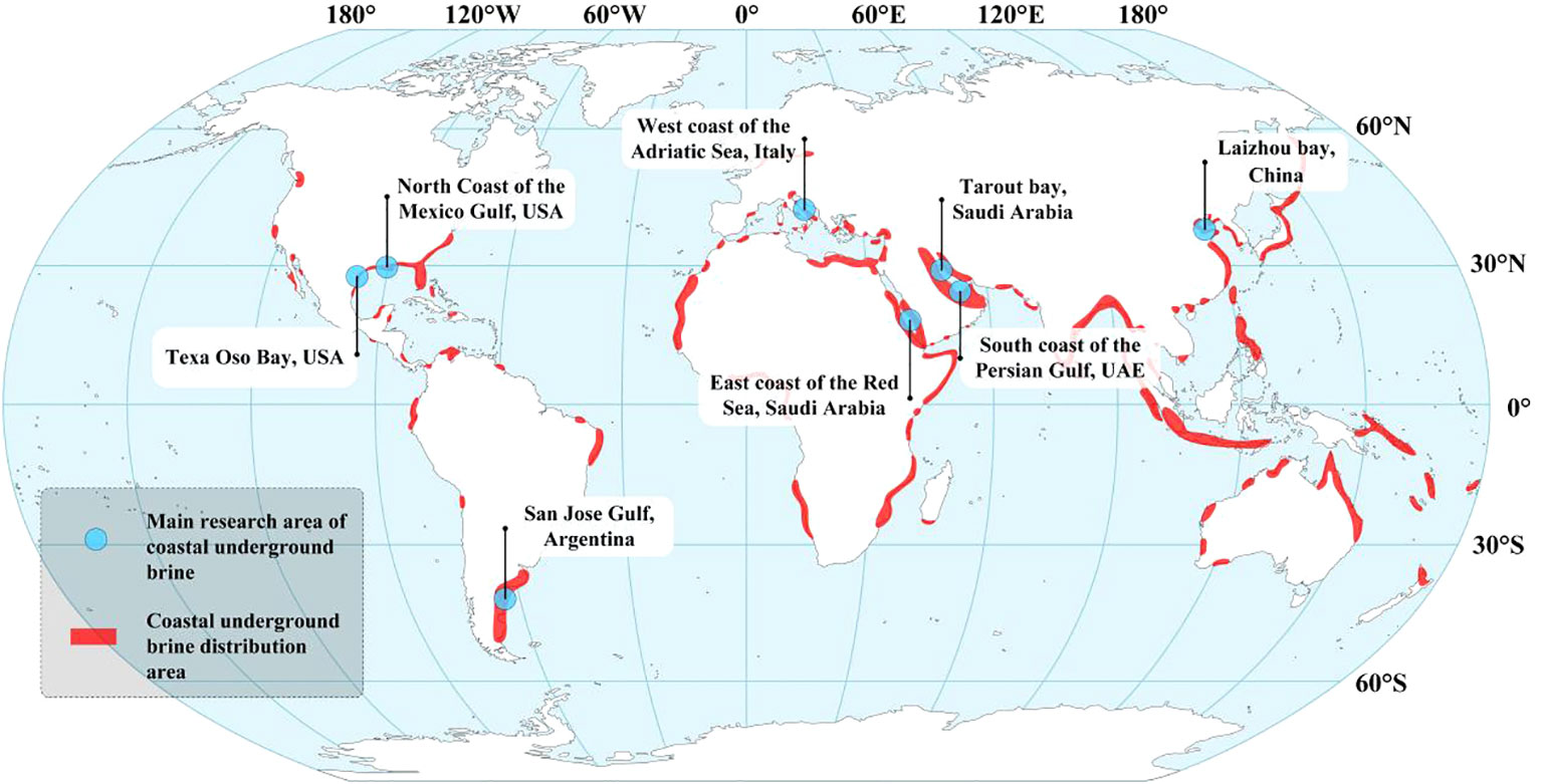
Figure 1 Distribution of the main worldwide coastal underground brine reserves and research areas (Sanford and Wood, 2001; Frank et al., 2009; Zhang, 2021).

The tidal flat represents a shallow coastal underground reserve of marine salt because of the evaporation that occurs (Han, 1996). Studies have shown that water and salt circulate between the seawater and shallow brine in mudflat areas with low-permeability surface sediments (10⁻⁷–10⁻⁵ m/s) during tidal action, although the rate of water and salt exchange is low (Ma et al., 2015; Hou et al., 2016; Ma, 2016; Zhang, 2021). In some coastal salt marsh or tidal flat areas, there are areas of high-permeability sediments that serve as biological channels, and provide preferential pathways for rapid exchange between seawater and groundwater, and where the salt content of porewater in the sediment matrix increases near the channels (Harvey and Nuttle, 1995; Escapa et al., 2008; Xin et al., 2009; Wilson and Morris, 2012; Xiao et al., 2019). There is an exchange process between the evaporated salt on the tidal flat surface and the shallow brine in the mudflat. During the rising tide, evaporated salt dissolves in seawater and is transported to the shallow brine in the mudflat, where high-salinity brine participates in the groundwater-seawater cycle and is released through the tidal flat during the ebb tide (Del Pilar et al., 2015; Hou et al., 2016; Zhang, 2021; Sun et al., 2023).

High-salinity brine that is buried in the lower intertidal zone is another source of marine salt for shallow coastal underground brine reserves. Coastal underground brine reserves have two favorable characteristics that mean they can receive salt from the marine environment. First, as a result of historical frequent marine transgressions and regressions, most coastal aquifer systems have interlayers of fine-grained and coarse-grained sediments, and, of these, the coarse-grained sand layers serve as interconnected aquifers between the tidal flat and the extraction areas. Driven by the tide, groundwater and solutes are periodically transported from the tidal flat area to the extraction areas (Yi et al., 2012; Fu et al., 2020). Second, where coastal underground brine has been extracted over the long term, the groundwater level may be lower than the sea level in the extraction areas and depression cones may have formed (Han et al., 2014; Liu, 2018; Qi et al., 2019). The hydraulic gradient between the marine and groundwater environments may also increase in arid climate conditions and storm surge events (William et al., 2008; Yang et al., 2015; Xing et al., 2023). When the groundwater flow field is influenced by these conditions, the high-salinity brine buried in the lower intertidal zone can continuously supply the extraction areas.

The salt in the aquitard can be considered as the third type of salt source that can supply coastal underground brine reserves. The salt stored inside the aquitards can be replenished to its adjacent brine layer through diffusion (Li et al., 2021). During the marine invasion and regression, aquitards gradually form during the formation of coastal underground brine. The total amount of salt stored in the aquitards is enormous, with a large amount of high salinity ancient seawater stored inside. At the same time, it continuously captures salt from the flowing recharge water and evaporated salt dissolved and infiltrated on the surface of the tidal flats (Gao et al., 2016; Li et al., 2021). From the perspective of high salinity water reserves in aquitards, they have enormous potential to recharge underground brine in coastal mining areas. However, the permeability of aquitards is low (10^-8−10^-10 m/s), and even if groundwater extraction increases its diffusion rate by hundreds of times, the rate of salt diffusion replenishing brine resources is still slow (Mongelli et al., 2013; Han et al., 2014; Larsen et al., 2017; Li et al., 2021). Therefore, during a short time scale (such as single or multiple tidal cycles), the release of salt from aquitards is very minimal, making it difficult to quickly and effectively replenish the underground brine resources in mining areas.

To sum up, although we have the theory of tidal flat halogenesis, information about the fate of evaporated salt on the tidal flat under tidal action, and various water-salt transport models that describe the processes in multiple tidally influenced coastal brine layers (Gao et al., 2016; Fu et al., 2020; Zhang, 2021), we do not have information about how the first two salt sources and tidal cycles influence the supply of salt to, and losses from, the shallow coastal groundwater in mining areas. To describe the above process, we need information about how the groundwater salinity evolves and how it is distributed in the tidal flat and coastal brine mining area during the tidal cycle.

The combination of in-situ hydrological parameter observation and numerical simulation is one of the main methods for exploring hydrological processes and pore water salinity distribution in tidal flats and salt marshes (Xiao et al., 2019; Fang et al., 2021, 2022; Shen et al., 2022; Shen et al., 2023; Zheng et al., 2023). However, the above research methods can not accurately depict the groundwater salinity distribution at different tidal times in complex stratigraphic environments with high resolution. With the upgrading of hydrogeophysical monitoring instruments and the optimization of geophysical data interpretation methods, the Electrical resistivity tomography (ERT) is widely used to monitor and research groundwater hydrological processes in in-situ coastal zones. ERT survey results from different times can provide information about brackish water and seawater intrusion processes that can be analyzed and used to establish different types of coastal seawater-groundwater exchange models (Franco et al., 2009; Misonou et al., 2013; Fu et al., 2020; Zhang, 2021; Zhan et al., 2023; Zhang et al., 2023). Further, the Archie formula, Manning formula, and the salinity box model can be combined to support quantification of the groundwater discharge and salt flux in the tidal flat area (Zhang K. et al., 2021; Zhang Y. et al., 2021, 2023; Xing et al., 2023).

In this study, we monitored the resistivity profiles in the brine mining area and tidal flat area through the tidal cycle using ERT technology. We then combined the monitoring results for groundwater levels within the tidal cycle, salinity, and conductivity of the water in the brine mining wells, and analyzed the salt supply and loss processes in the shallow coastal groundwater in the chosen mining area.

2 Study area

The study area is on the southern coast of Laizhou Bay, in the northern part of Shandong Province, China. We did a survey that extended across the land-based brine extraction area and the tidal flat (Figure 2). The terrain on the land-based area is flat. The marine area consists of muddy sandy tidal flats that have a gentle slope of less than 3‰ and surface sediment that has a permeability coefficient of approximately 10⁻⁵ m/s. There are multiple brine extraction wells operating 24 hours per day on the land-based area.

Figure 2

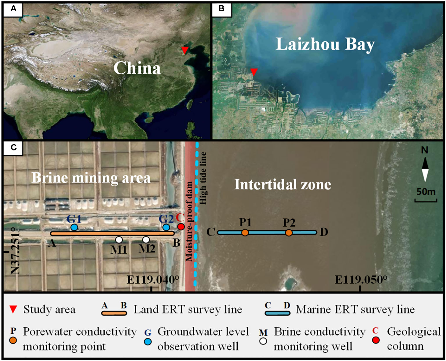
Figure 2 Map of the study area. (A, B) Location of the study area on the south coast of Laizhou Bay, East China. (C) The fieldwork layout in the brine mining area and the intertidal zone, including two ERT monitoring lines, two groundwater level observation wells, two brine sampling wells, one geological borehole, and two tidal flat pore water conductivity monitoring points.

The study area is characterized by irregular semidiurnal tides, and the average tidal range is approximately 0.9 m. The average flood tide duration is 6 h 22 min, and the average ebb tide duration is 6 h 6 min (Zhang, 2021).

Within the study area, there are three horizontal layers of brine. The upper and lower layers have low salinity, while the middle layer has high salinity (Zheng et al., 2014; Gao et al., 2016; Qi et al., 2019). These brine layers formed during the early Pleistocene period of the Cangzhou transgression, the late Pleistocene period of the Xianxian transgression, and the early Holocene period of the Huanghua transgression. The underground brine that formed during the Huanghua transgression is composed of groundwater brine that was deposited during the late Holocene. The total dissolved solids (TDS) of the brine ranges from 50 to 140 g/L (Gao et al., 2016).

The study area is on the marine-side boundary of the brine precipitation funnel. The observation results from June 2022 of 16 groundwater level observation logs in the Yangkou Salt Field and the surrounding area showed that (Figure 3A) the groundwater level rapidly decreased to −35 m over 7 km in a southwest direction from the research area. There is a significant hydraulic gradient between the nearshore research area and the inland extraction area, and groundwater from the tidal flat area continuously flows toward the landward side of the brine precipitation funnel. The two monitoring sections in this study were set up at an angle of approximately 36° with the groundwater flow direction. In July 2022, the groundwater levels at observation wells G1 and G2 in the extraction area were approximately −7.9 m and −5.2 m, respectively.

Figure 3

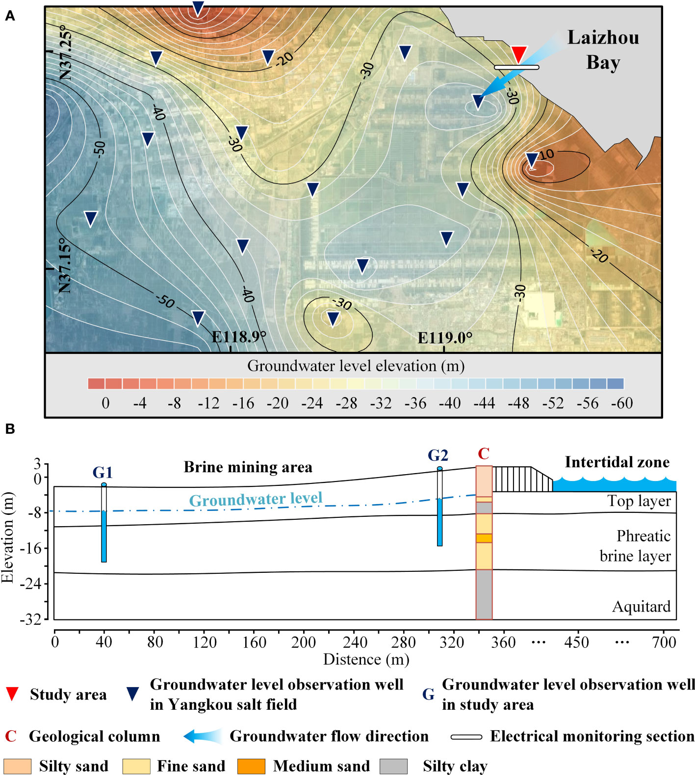
Figure 3 (A) The average groundwater level in the study area in June 2022. (B) Hydrogeological profile along the survey line in the study area.

The stratigraphic information for geological borehole C within the research area (Figure 3A) shows that, from shallow to deep, the aquifer can be divided into a fine-grained sediment cover layer (top layer), a phreatic brine aquifer layer that is about 14 m deep (middle layer), and a weakly permeable aquitard (bottom layer).

3 Materials and methods

3.1 Measurement of the conductivity and salinity of the seawater and underground brine

The seawater conductivity data were used to determine the electrical resistivity values within the seawater grid during the inversion of the ERT data, and to investigate the recharge relationship between the seawater and the subterranean brine. Seawater samples were collected from the endpoint of the marine ERT survey line and the conductivity of the samples was measured at the same time as the ERT measurements were taken. The brine conductivity and salinity data were used to validate the accuracy of the ERT inversion results and to calculate the salt flux of subterranean brine in the extraction area. Subterranean brine was extracted at M1 (150 m from point A) and M2 (225 m from point A) on the land ERT survey line (Figure 2C). The sampling depth was at a depth of approximately −10 m, and samples were collected for conductivity measurements over three consecutive tidal cycles. The conductivity of the water was measured with a water quality meter (AZ8362).

3.2 Porewater conductivity monitoring

The conductivity of the porewater in the intertidal sediments was measured at two points, at 530 m and 610 m, along the marine ERT survey line using a multi-parameter automatic monitor (Solinst LTC Levelogger Edge). The monitoring probe was wrapped with multiple layers of gauze to ensure it would not get blocked by sediment, and buried at a depth of 1 m. Data were collected every 0.5 h. This monitoring was done at the same time as the ERT monitoring.

3.3 Groundwater level monitoring

Two groundwater observation wells (G1 and G2) were installed along the land ERT survey line to measure the groundwater level (Figure 3B). The groundwater levels were measured at a time interval of 0.5 h using a steel tape water level meter with a resolution of 1 mm (Yingtianliang Company). Again, these measurements were done at the same time as the ERT survey.

3.4 ERT survey

The land ERT survey line (A–B) and marine ERT survey line (C–D) were along the vertical coastline (Figure 2). The monitoring results were analyzed to identify the salinity variations in the aquifer between the marine area and the tidally influenced brine extraction areas. The land and marine ERT measurements were done simultaneously in July 2021.

3.4.1 Data acquisition

The ERT monitoring system (GEOPEN) used to monitor the land and marine areas consisted of an E60DN mainframe, a booster, and intelligent cables (with stainless steel electrodes). The terrestrial ERT monitoring system had cables with electrodes spaced at 5 m intervals. There were 64 electrodes altogether, and the total cable length was 315 m. The marine ERT monitoring system had cables with electrodes every 2.5 m. There were 100 electrodes, and the total cable length was 247.5 m.

The ERT measurements for the land and marine areas should have been taken at the bottom boundary of the subaqueous brine layer (elevation approximately −20 m). These measurements were taken with a Wenner-Schlumberger array; this equipment is widely used in coastal groundwater hydrological monitoring and is known for its large detection depth, high vertical resolution, and strong anti-interference ability (Hermans and Paepen, 2020; Wu et al., 2021). The array is powered by a 24V battery pack, and the user-defined maximum current is 1A and the power supply time is 1 s. The ERT measurements of the land and marine areas started synchronously, and the data acquisition took approximately 30 min.

The electrode layout methods proposed by Zhang Y. et al. (2021) and Xing et al. (2023) were consulted to find out how to prevent the electrode positions of the cables for the marine ERT monitoring from drifting under tidal influence. A 30-cm deep trench was excavated for the cables during low tide, three days before the monitoring work started, and the cables were placed in the trench and covered with sediment in situ.

The saturation of the sediment at 0, 80, 160, and 240 m deep where the electrodes of the marine ERT cable were located was measured at low tide. The saturation ranged from 97.1% to 99.8%. We concluded that the environment in which the electrodes of the marine ERT cable were placed was stable and that the sediment remained saturated during tidal cycles.

3.4.2 Data processing and inversion

The resistivity profile data were checked for quality and data points in the resistivity data that were more than three times greater or less than the adjacent data were removed. Less than 1% of the total resistivity data were removed in this process (Wu et al., 2021). The apparent resistivity values were converted to true resistivity values by time-lapse inversion. The ERT data were analyzed using the least squares method with RES2DINV software v.4.05.30 (Geotomo Inc.) (deGroot-Hedlin and Constable, 1990). The terrain elevation data and the corresponding seawater resistivity and sea level elevation data had to be combined before the resistivity data set was inverted. When calculating the inversion, RES2DINV performs terrain modeling, calculates the water layer thickness, establishes a simulation domain, and divides it into finite element grids. The resistivity between the beach surface and the sea level was calculated from the seawater resistivity. In this study, the seawater resistivity was based on the monitoring data.

The quality of the inversion result was evaluated by checking the Abs error (absolute error) between the measured and predicted apparent resistivity values. It is generally accepted that inversion results have more credibility when the absolute error is below 10%. However, an absolute error that is too low may lead to overfitting and data inconsistency (Dimova et al., 2012). Therefore, in this study, the absolute error was controlled at around 10%.

3.4.3 Inversion model appraisal

The depth-of-investigation (DOI) index is used to analyze the influence of inversion parameters on the model and evaluate the reliability of the inverted resistivity data (Oldenburg and Li, 1999; Paepen et al., 2020; Zhang Y. et al., 2021). The DOI index is calculated using Equation 1.

$\begin{array}{ll}DOI=\frac{\left|\log R_{inv,1}-\log R_{inv,2}\right|}{2}& (1)\end{array}$

It is calculated based on two additional inversions (R_inv,1 and R_inv,2, which are inverted resistivities) using two reference models (R_app,1 and R_app,2) which are 0.1 and 10 times the average observed apparent resistivity of the datasets (Oldenburg and Li, 1999; Paepen et al., 2020; Zhang Y. et al., 2021).

3.4.4 Reliability analysis of inverted resistivity

The expected resistivity (R_p) of the sediments at the sampling or monitoring locations was calculated from the monitoring data for the conductivity of the submarine brine and of the porewater of tidal flat sediments. The numerical values and variations of R_p and the ERT inversion results (R_inv) were compared to verify the accuracy of the ERT inversion data.

Based on Archie’s law (Archie, 1942) and the resistivity of the brine sample (R_w), the expected resistivity (R_p) of the sediments at the sampling points of the coastal mining area (M1, M2) can be calculated as follows:

$\begin{array}{ll}{R}_p=\frac{a·R_w}{{\varphi }^m}& (2)\end{array}$

Where a is a tortuosity factor, m is a cementation factor, and ϕ is the porosity. The values of the porosity and rock electrical parameters were based on the results of testing the porosity of the sediment samples and empirical values of the electrical parameters for medium to fine sand layers (Jackson et al., 1978; Zhang et al., 2004; Zhang Y. et al., 2021). Here, ϕ=0.4, a=0.6, and m=1.4.

The resistivity of the sediments will be affected by a high clay content in the muddy tidal flat sediments because of the influence of the surface conductivity and pore fluid conductivity (Revil, 2013). The effects of the surface conductivity and R_w on the resistivity of the sediments can be separated with a modified version of Archie’s law (Equation 3) that was proposed by Nguyen et al. (2009) and Shao et al. (2021). Therefore, the expected resistivity (R_p) of the sediments at the monitoring points (P1, P2) can be calculated based on R_w, as follows:

$\begin{array}{ll}{R}_p=\frac{1}{{(F^{\text{'}}{R}_w)}^{-1}+b}& (3)\end{array}$

Where F’ represents the effective layer factor, and b represents the contribution of the surface conductivity to ρ, independent of the fluid conductivity. The parameters in Equation 3 were set based on the preliminary results from Zhang’s (Zhang, 2021) study of the muddy tidal flats on the south coast of Laizhou Bay. F’ was set to 2.5, and b was set to 0.335.

The resistivity data from four of the inversion calculation grids near the brine sampling points and two of the inversion calculation grids near the porewater conductivity monitoring points in the tidal flat sediments were extracted and their average values were calculated using the R_inv data extraction method of Zhang Y. et al. (2021) and Xing et al. (2023). The output from R_inv was then compared with the R_p calculated using Equations 2, 3 to determine the reliability of the ERT inversion results.

3.5 Calculation of the salt flux

The brine occurs in a water-bearing fine sand layer in the monitoring area, and its fluid movement follows Darcy’s law. Therefore, the water flux passing through the monitoring section along the groundwater flow direction can be expressed by the basic flow equation and Darcy’s law, as follows:

$\begin{array}{ll}Q=A\sin \theta \times v& (4)\end{array}$

$\begin{array}{ll}v=K\frac{\text{Δ}h}{L\cos \theta }& (5)\end{array}$

Where Q is the flow rate (m³/s), A is the underground brine flow area divided based on the ERT monitoring result (m²), Asinθ is the underground water flow area perpendicular to the flow direction, v is the flow velocity (m/s), and K is the permeability coefficient (m/s), which was taken as 1×10⁻⁴ m/s in this case (Guo, 2018; Chang, 2018). Δh is the hydraulic head difference (m) between G1 and G2, L is the length of the ERT monitoring section in the brine extraction area (m), and θ is the angle between the flow field and the monitoring section (θ=36°).

By combining the Equations 4, 5 and salinity, density, and volume calculation equations (Equations 6–8), the salt flux passing through the monitoring section along the groundwater flow direction can be calculated using Equation 9, as follows:

$\begin{array}{ll}S=\frac{m_s}{m_w}& (6)\end{array}$

$\begin{array}{ll}{m}_w=\rho V& (7)\end{array}$

$\begin{array}{ll}V=Q\times \text{Δ}t& (8)\end{array}$

$\begin{array}{ll}{m}_s=\frac{S\times \rho \times \text{Δ}t\times A\text{sin}\theta \times K\times \text{Δ}h}{L\cos \theta }& (9)\end{array}$

Where S represents the salinity of the brine (g/kg), m_s represents the mass of salt (g), m_w represents the mass of brine (kg), and ρ represents the brine density (kg/m³), which was assumed to be 1.08×10³ (kg/m³). V represents the brine volume (m³) and Δt represents the time interval for sampling underground brine (s).

4 Results

4.1 Groundwater parameters

The water levels measured at the G1 and G2 groundwater monitoring wells followed a similar pattern (Figure 4). The groundwater level remained stable during the transition from low tide to high tide. The groundwater level increased slightly by less than 10 cm within 2 hours of the high tide. More than 2 hours after the high tide, the groundwater level started to decrease until the seawater receded, and the groundwater level returned to the pre-tidal level.

Figure 4

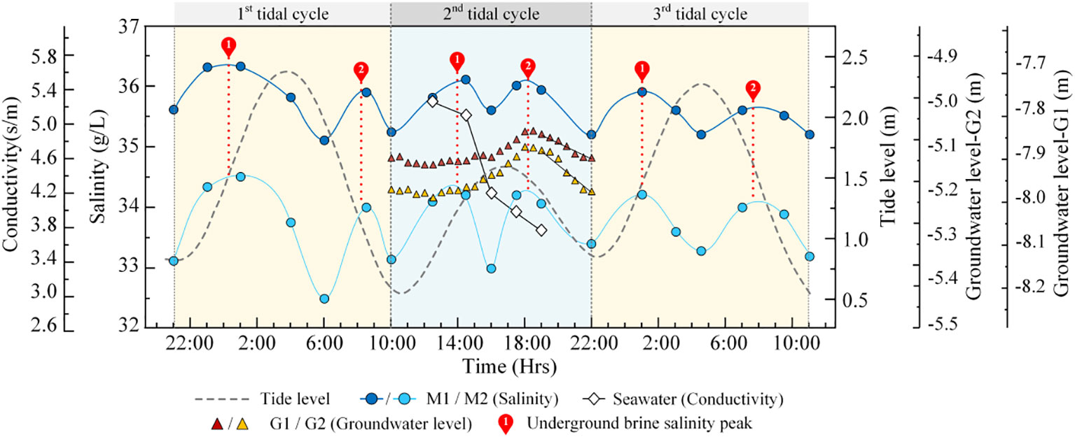
Figure 4 Underground brine salinity, groundwater level, and seawater conductivity in the mining area during tidal cycles (the blue area represents the ERT monitoring period, the 2^nd tidal cycle).

The salinity of the brine water followed a specific pattern during the three tidal cycles of the monitoring period (Figure 4). Within each tidal cycle, the salinity increased and decreased twice, producing two salinity peaks. The two salinity peaks occurred during the rising and falling tides of the same tidal cycle, at a time interval of approximately 5−7 hours (from low tide to low tide).

The conductivity was positively correlated with the salinity and reflected the changes in the seawater salinity. The seawater conductivity reached a peak after the seawater covered the tidal flat, but the conductivity of the seawater on the tidal flat decreased as the tide continued to rise. The conductivity values decreased until the seawater receded from the study area.

4.2 ERT inverted resistivity

4.2.1 Accuracy verification of the resistivity data

The R_p and R_inv values in the surface sediments of the tidal flats followed a similar pattern during the tidal cycle. The R_p and R_inv showed an overall decrease during the rising tide, and were lowest before the high tide. The R_p and R_inv then increased during the ebb tide (Figure 5A). The R_p and R_inv data for the brine mining area showed relatively little, but consistent, variation during the tidal process, which indicates that the underground brine area was relatively stable during the tidal cycle. During the flood tide, the R_p and R_inv values first decreased and then increased, and the resistivity values were lowest when the tidal flat was submerged by seawater. During the ebb tide, the R_p and R_inv values also decreased first and then increased, and the resistivity values were lowest after the high tide (Figure 5B). Overall, the R_p values showed less fluctuation than the R_inv values, but the values were generally close (Figures 5A, B). These results suggest that R_inv accurately reflects the variations in the porewater salinity.

Figure 5

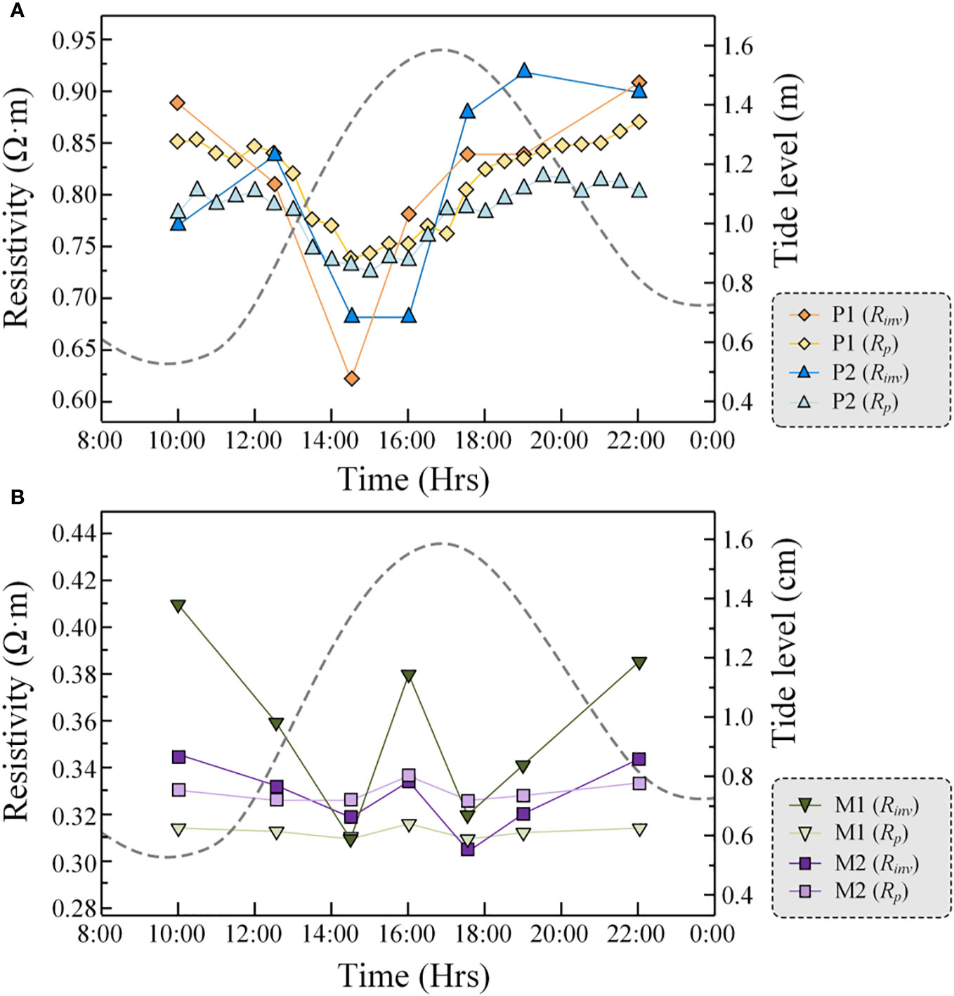
Figure 5 Changes in the expected resistivity and inverted resistivity in sediments in the tidal flat (A)/brine mining area (B) during the tidal cycle.

4.2.2 Quality appraisal

A low DOI index is obtained when the resistivity structures in the model are driven by the data and not by the inversion process, which is influenced by the reference model (Paepen et al., 2020; Zhang et al., 2023). All cells with a DOI index greater than 0.2 were considered as less reliable (Thompson et al., 2017). In this study, nearly all of the DOI index values of the ERT inverted result are less than 0.1. Only a small portion of the DOI index values of marine ERT inverted results in deep regions is between 0.1 and 0.15 (Figure 6). Therefore, all inversions are adequately sensitive to characterize the general sediment resistivity distribution in the studied area.

Figure 6

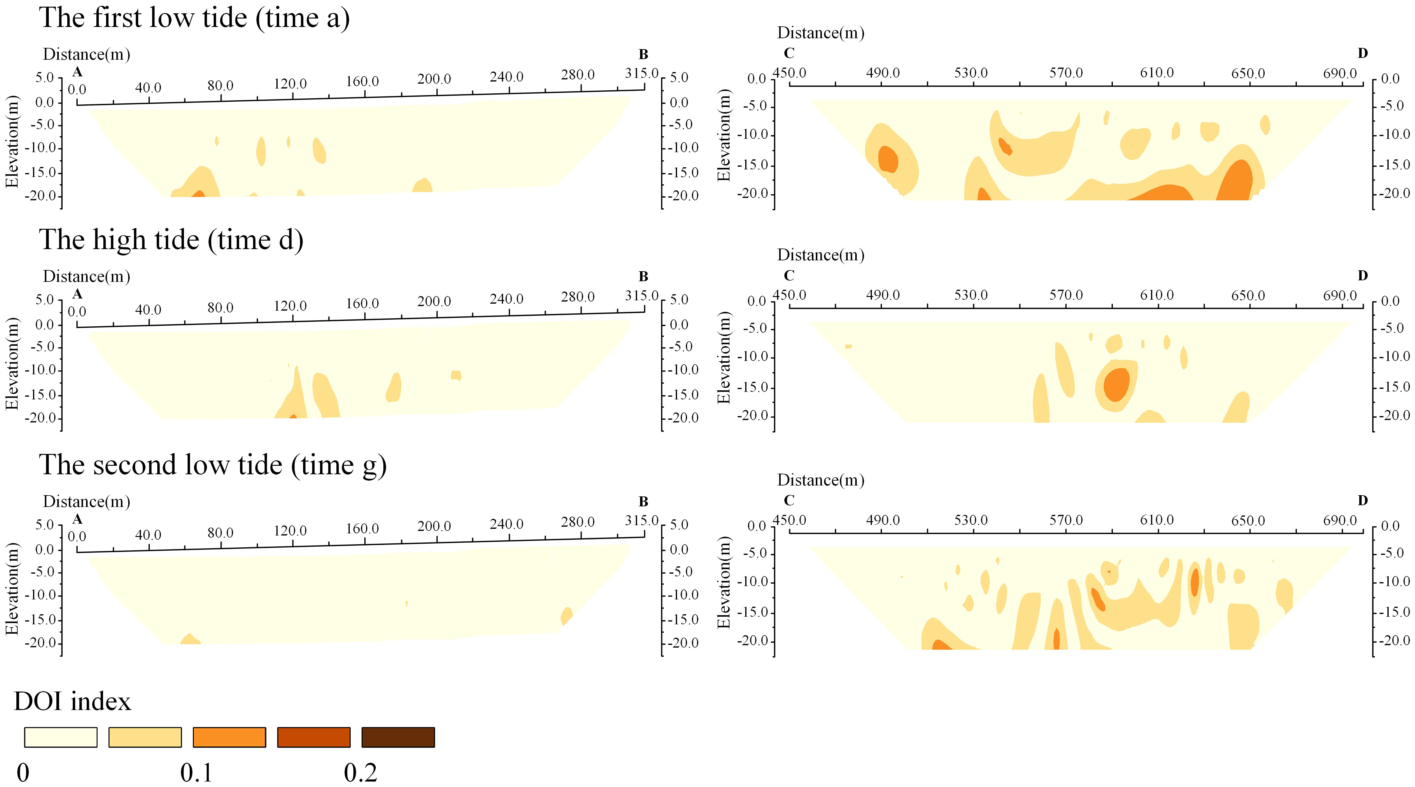
Figure 6 DOI index profiles for validating the effectiveness of inversion models. Here we only show the DOI index profiles of time a, d, and g, while the DOI index distribution patterns of other times are basically similar to the displayed profiles. (A–D) are the starting/ending points of land ERT survey line and marine ERT survey line respectively.

4.2.3 Variations in the inverted resistivity image during the tidal cycle

The average resistivity of the underground brine was 0.144 Ω·m. This value was substituted into Equation 2 and the expected resistivity of the brine zone was calculated as 0.32 Ω·m. This expected resistivity value was used as a standard to delineate the brine occurrence areas in the inversion resistivity profile. The top boundary of the brine body was generally consistent with the groundwater level. The distribution of the brine body remained relatively stable within the tidal cycle and occurred between -22 and -8 m, which was consistent with the distribution range of the brine layers from the geological column (Figures 3B, 7, 8).

Figure 7

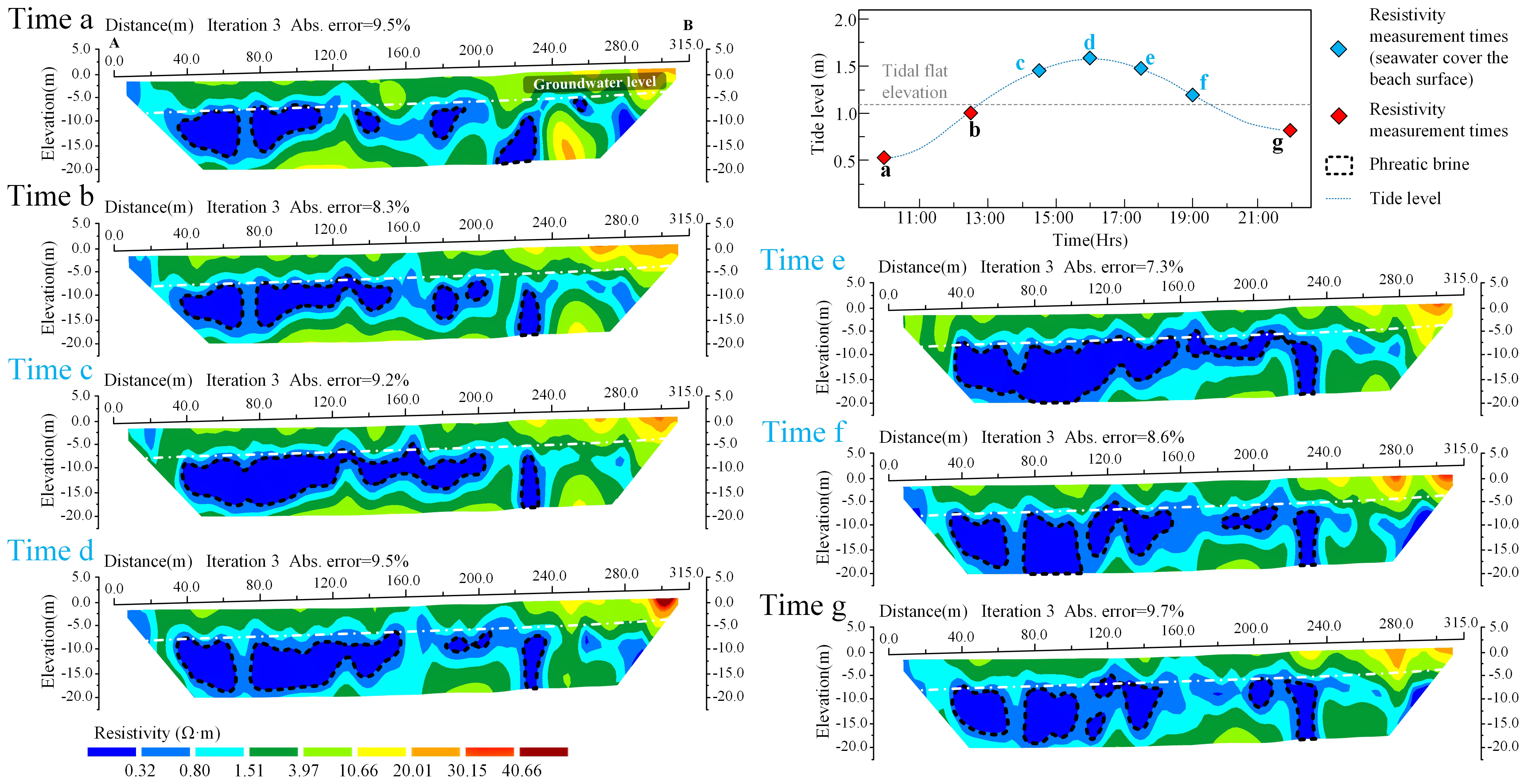
Figure 7 ERT inverted resistivity profiles during the tidal cycle in the brine mining area (AB line).

Figure 8

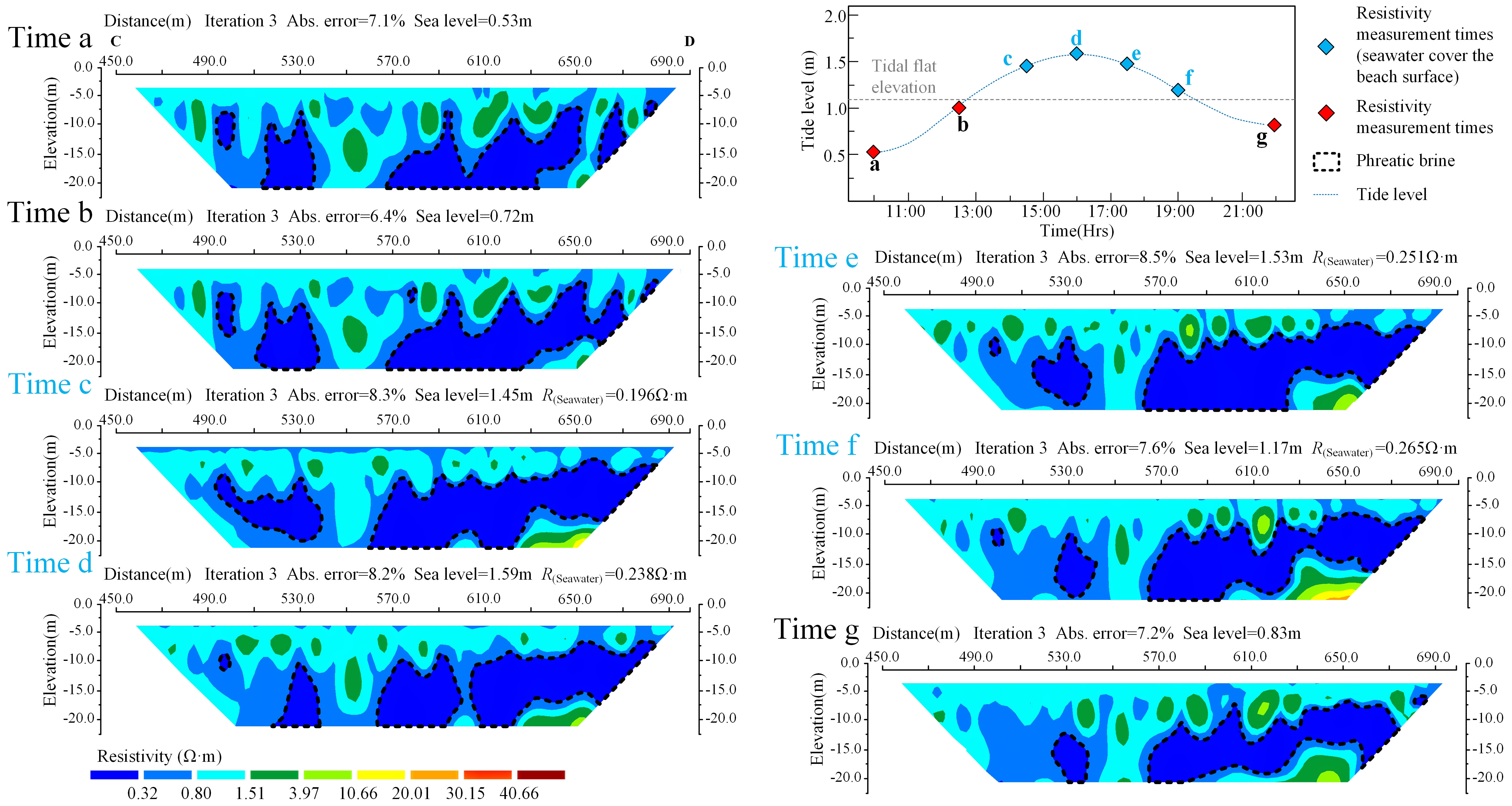
Figure 8 ERT Inverted resistivity profiles during the tidal cycle on the tidal flat (CD line).

The extent of the underground brine body followed two expansion and contraction cycles within the tidal cycle. During the rising tide, when the surface of the tidal flat was not covered by seawater (time a−b), the brine body in the mining area expanded, and the underground brine in the intertidal zone remained relatively stable. After the tidal flat was submerged in seawater (time c), the extent of the brine body in the mining area and the intertidal zone expanded significantly. During this stage, several anomalous low resistivity zones (< 0.8 Ω·m) that connected the tidal flat and the brine body appeared in the intertidal zone. During high tide (time d), the extent of the underground brine generally decreased, and most of the anomalous low resistivity zones that connected the brine body and the tidal flat in the intertidal zone disappeared. In the early stage of the ebb tide (time e), the underground brine body expanded again, and then shrunk during the subsequent ebb tide (time f−g). After the seawater receded from the tidal flat, the anomalous low resistivity zones connecting the brine body and the tidal flat in the intertidal zone completely disappeared (Figures 7, 8).

5 Discussion

5.1 Salt transport flux in the coastal brine mining areas during the tidal cycles

We calculated the amount of salt transport (m_s) and the transport rate (Rs) in the underground brine bodies at different times during a single tidal cycle using Equation 9, the data for the extent of the brine body, and other results from the inversion of the ERT resistivity data (Figure 9; Table 1).

Figure 9

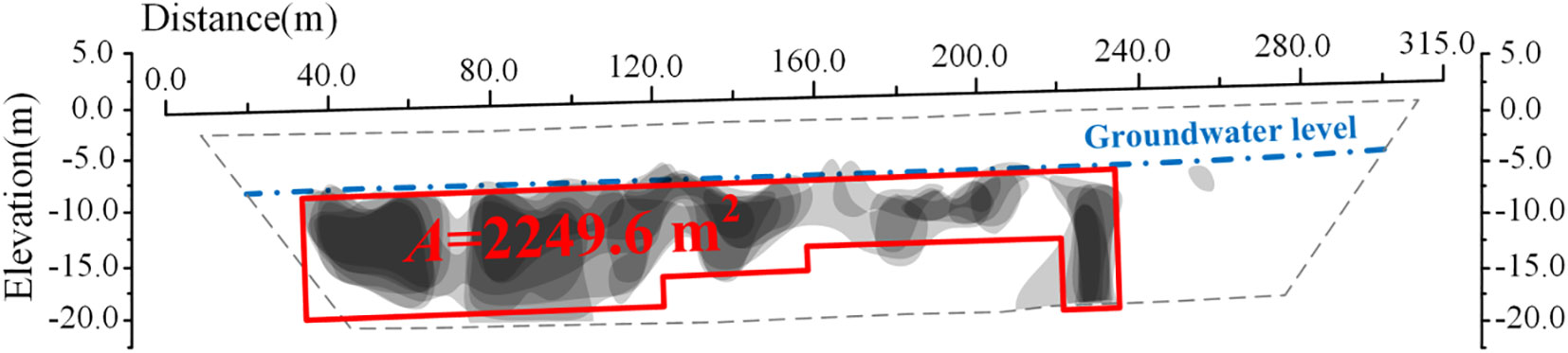
Figure 9 The distribution of the underground brine within the ERT monitoring profiles in the brine mining area. The gray shadow represents the extent of the underground brine at different tide times, which was divided using the ERT inverted resistivity profile data. The red box represents the range of the underground brine flow area that was involved in the calculation of the salt transport flux (A=2249.6 m²).

Table 1

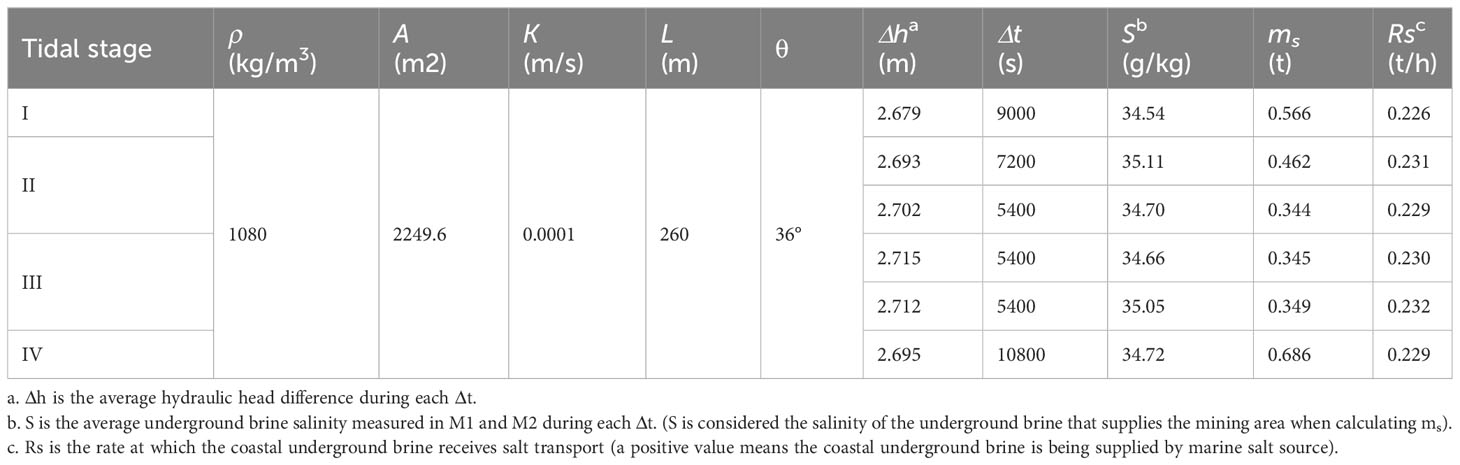
Table 1 Calculation parameters and the results of the salinity transport flux.

The coastal brine extraction area is at the marine boundary of the precipitation funnel (Figure 3A). The groundwater head difference between G1 and G2 (2.679−2.715 m) and the salinity of the underground brine (34.54−35.11 g/kg) did not fluctuate significantly as the tides fluctuated and when influenced by the large hydraulic gradient from the sea to the land, continuous brine extraction, and low permeability of the sandy tidal flats. This indicates that the underground brine in the coastal extraction area was constantly receiving a stable supply of salt from the marine environment. The results show that the salt was entering the brine body through the monitoring section at a rate of 0.226−0.232 t/h, which means that the total salt flux entering the underground brine bodies over a vertical flow area of 1322.3 m² (Asinθ) was 2.75 t during a single tidal cycle or 5.50 t each day. The brine extraction wells in this area are pumped at a rate of approximately 5.5 m³/h, which means that approximately 4.98 t of salt can be extracted per day. In an ideal scenario (assuming consistent tidal fluctuations and that the brine layer distribution in the monitored area remains the same), the daily salt supply replenished to the brine extraction zone along a 150 m (Lsinθ) coastline can approximately sustain the extraction capacity of one brine well.

5.2 The salinity of the marine salt source supply to the coastal underground brine in the mining area

In the study area, water and salt from the marine environment continuously migrate into the underground brine layer in the extraction area under the combined influence of the seaward groundwater flow and tidal action. The rise and fall of Rs can reflect any changes in the water-salt migration state. The head difference (Δh) between G1 and G2 and the salinity (S) of the water replenishing the underground brine in the extraction area are the main factors that affect the water-salt migration rate (Rs) (Equation 9; Table 1). Although the ranges of the Δh and S values in the study area were small (Figure 10), these data can still indicate the water-salt migration state in the brine layer of the extraction area during different tidal stages.

Figure 10

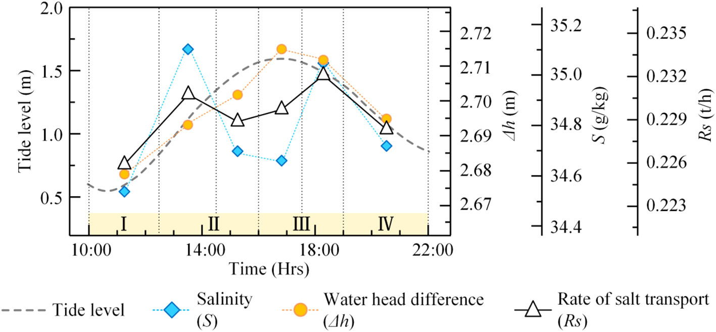
Figure 10 The relationship between the salinity, hydraulic head difference, and the salt transport rate. The yellow boxes show the four stages of salt transport during the tidal cycle (I−IV), namely, (I) the early stage of the rising tide, when the seawater did not cover the beach surface; (II) the rising tide, when the seawater covered the beach surface; (III) the early stage of the ebb tide, when seawater still covered the beach surface, and (IV) the ebb tide, when the seawater receded from the beach surface.

In coastal aquifer systems, the groundwater salinity generally shows a single salinity peak with a time lag relative to the tides during the tidal cycles (Hou et al., 2016; Zhang et al., 2023). However, in this coastal brine extraction area, the groundwater salinity showed two salinity peaks. Fu et al. (2020) also observed two peaks in the groundwater salinity at northern Changyi Beach, which is also located on the southern coast of Laizhou Bay. This suggests that there are at least two pathways for salt transport from the marine environment to the coastal brine reserves in this region. There is also a stable pathway for salt loss in this area, i.e., the extraction of underground brine. Here, we combined the patterns of the low-resistivity anomaly distribution in the ERT inversion resistivity profiles, and identified four stages in the marine salt supply, as follows:

Stage I (the early stage of the rising tide, when the seawater did not cover the beach surface). The underground brine in the extraction area is replenished from the lower part of the tidal flat (Del Pilar et al., 2015; Guo, 2018; Fu et al., 2020), and the salinity increases and the brine distribution range expands slightly on both the sea and land sides (Figures 4, 7, 8, 11A). During this stage, there is a time lag of several hours between the groundwater level and the tide (Gao et al., 2010; Su et al., 2018), and the rise in the tide does not cause changes in the groundwater levels of G1 and G2 (Figure 4). Δh stays the same, so the increase in S is the only factor that contributes to the increase in Rs (Figures 4, 10).

Figure 11

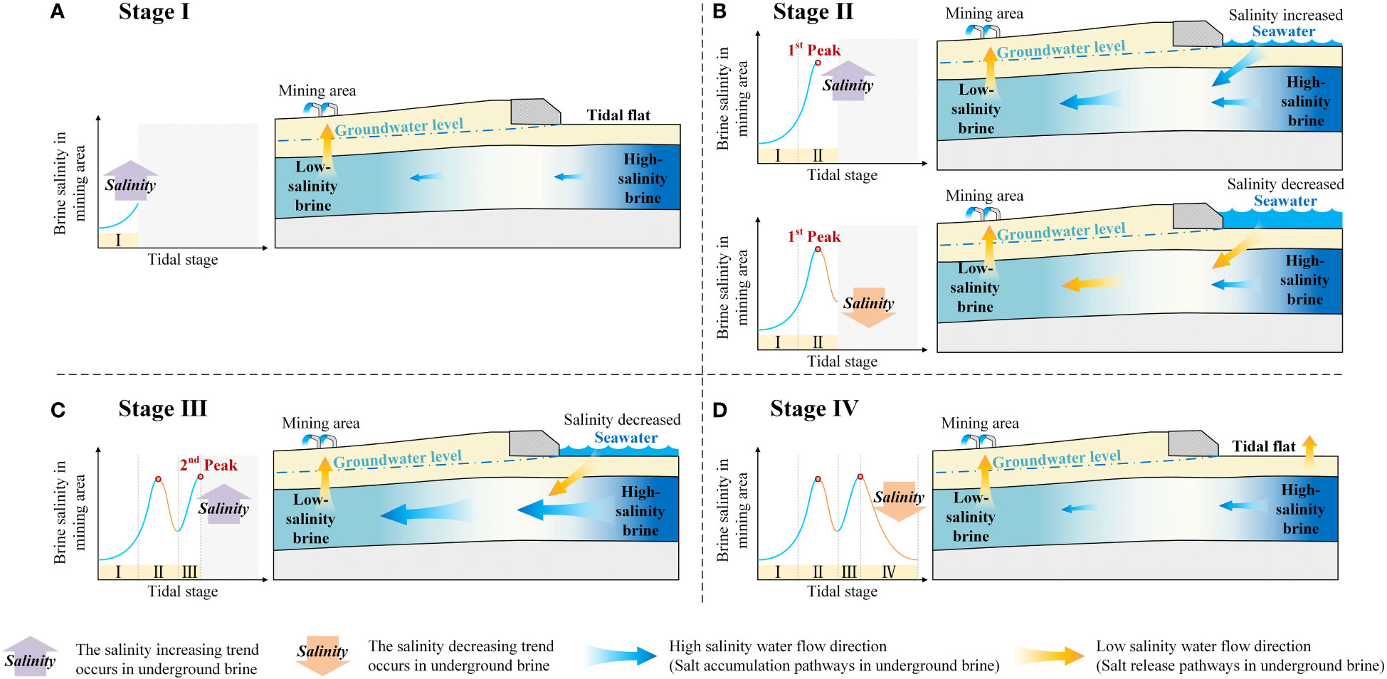
Figure 11 The two salinity peaks mode of marine salt source supplementing coastal underground brine during a single tidal cycle. (A−D) show the salt accumulation and pathways where underground brine is lost in mining areas during the tidal cycle (stages I−IV). The blue/yellow arrows represent the flow direction of water with different salinity that cause the accumulation/loss of salt in underground brine resources compared to the previous stage or the previous moment in the same stage.

Stage II (during the rising tide, when the seawater covers the beach surface). In the early stage of stage II, the brine in the mining area is replenished from the lower part of the tidal flat and the high-salinity water infiltrating from the surface of the flat. The first salinity peak appears in the underground brine of the mining area (Figures 4, 10, 11B), and the extent of the brine area on the sea and land sides significantly expands (Figures 7, 8). The increase in Rs is caused by the increase in Δh and S. Because G2 is closer to the marine environment than G1, the groundwater level at G2 fluctuates slightly more than that at G1, which results in an increase in Δh (Figure 4). The value of S increases because of the dissolution of a large amount of evaporite salt after the tidal flat is submerged by seawater, and these high-salinity water bodies infiltrate into the aquifer system through bioactive channels or high-permeability sediment distribution zones near the coast (Del Pilar et al., 2015; Hou et al., 2016; Xiao et al., 2019). The ERT inversion resistivity profiles for the marine side show there are anomalous areas of low resistivity that connect the brine bodies and the tidal flat, which suggests that there are preferential pathways for high-salinity water replenishment (Figures 7, 8).

In the late part of stage II, a large amount of low-salinity seawater infiltrates from the surface of the flat, leading to a decrease in the salinity of the underground brine (Figures 4, 11B), and the extent of the brine on the sea and land sides decreases (Figures 7, 8). Although Δh continues to increase during this period, the rapid decrease in the seawater salinity leads to a significant reduction in S, and Rs shows an overall decrease (Figures 4, 7, 8, 10). The infiltration of low-salinity water through the flat restricts the amount of replenishment of high-salinity water from the lower part of the tidal flat to the brine mining area to some extent.

Stage III (the early stage of the ebb tide, when the seawater still covers the beach surface). A large amount of high-salinity water is transported from the sea to the land through the aquifer in a horizontal direction into the underground brine reserve in the mining area. The second salinity peak appears in the underground brine in the mining area (Figures 4, 10, 11C), and the extent of the brine expands again on the sea and land sides (Figures 7, 8). Because of the time lag, the pumping intensity of the tidal action peaks in this stage (Santos et al., 2011), and the groundwater levels at G1 and G2 and the head difference Δh all reached their peak values. The salinity S also reached its peak value synchronously. This means that a large amount of high-salinity water from the lower part of the tidal flat is transported into the underground brine in the mining area under the tidal driving force during this stage. The intruding low-salinity seawater no longer controls the salinity of the underground brine in the mining area.

Stage IV (during the ebb tide, when the seawater recedes from the beach surface). In this stage, the tidal action weakens and high-salinity groundwater is discharged to the beach (Hou, 2016; Guo, 2018; Zhang, 2021), leading to a synchronous decrease in Δh and S, and a decrease in Rs (Figures 4, 10). The intensity of the seawater supply from the marine to the brine in the mining area weakens, and the salinity of the underground brine in the mining area begins to decrease (Figure 4). The extent of the brine gradually narrows on both the sea and land (Figures 7, 8, 11D).

We also observed that S has more influence on Rs than Δh. First, during the tidal cycle, the pattern of fluctuations of Rs is more similar to pattern of the fluctuation of S than Δh. Rs and S have two peaks, which occur early in stage II and late in stage III. Second, from late in stage II until early in stage III, S decreases while Δh increases, leading to an overall decrease in Rs. This implies that the two salinity peaks in the underground brine extraction area depend on the salinity of the different salt sources during each tidal stage. Therefore, for two salinity peaks to occur during a single tidal cycle in the brine extraction area (1) there must be at least two salt sources for the brine extraction area, and (2) each source must have a high value at different stages in the tide.

When the brine extraction area is adjacent to areas with strong evaporation, such as salt marshes, tidal channels, high tide line areas, and areas with a distribution of high-salinity underground brine, condition (1) is satisfied. When there are localized high-permeability zones in muddy tidal flats and the tidal flats are long enough, condition (2) is satisfied. This is because the wide and gentle tidal flats exacerbate the time lag of the groundwater level fluctuations caused by tidal action (Gao et al., 2010; Su et al., 2018). The peaks in the horizontally transported flux of salt from the sea to the land in the shallow aquifer will occur several hours after the high tide. The rising tide can quickly submerge a large area of the tidal flats and transport large quantities of dissolved evaporated salt to the nearshore side through the flats. This flow can supply the underground brine reserve when it crosses high-permeability zones (Stahl et al., 2014; Xiao et al., 2019; Zhang, 2021; Zhang et al., 2023). The flux of salt transported to the extraction area through this pathway will peak earlier than the high tide.

6 Conclusions

The marine environment is the main source of salt for the underground brine reserves adjacent to tidal flats. In this study, ERT monitoring sections and hydrology monitoring holes were established in the in-situ coastal area to evaluate the salt flux and pattern of salt recharge from marine salt source to mining areas through coastal aquifers. Based on the monitoring results, we developed a new method to quantify the replenishment of salt from marine salt source through the coastal aquifer to the underground brine in the mining area; We also found that there are two tidal-driven salinity peaks in the salt supply for the underground brine reserve in the coastal mining area during a single tidal cycle. The main findings are as follows:

(1) The coastal brine exploitation area is located at the boundary of a precipitation funnel. The salinity of the underground brine and the pre-existing large hydraulic gradient from the sea to the land are not significantly affected by fluctuations in the tidal level. The underground brine reserve in the mining area consistently receives a stable supply of salt from the marine, at a rate of 0.226−0.232 t/h. The total salt flux entering the underground brine reserve via a 150 m long shoreline and a 1322.3 m² window flow is 5.50 t per day, which roughly equates to the daily extraction of one brine well.

(2) During a single tidal cycle, there were two salinity peaks in the supply to the underground brine reserve. For this to happen, there must be at least two sources supplying brine to the mining area, and the salinity of the different salt sources is high at different tidal stages. We observed that the first salinity peak occurred after the initial stage of the rising tide when the seawater inundated the tidal flat (Stage II early). During this stage, seawater dissolves and carries a large amount of evaporated salt and transports it to the brine layer through high-permeability zones or bioactive channels, ultimately supplying the mining area. Late in Stage II, the seawater salinity decreased and the salinity peak disappeared. The second salinity peak occurred during the early stage of the falling tide (Stage III). The flow of high-salinity brine in the lower part of the intertidal zone accelerated toward the mining area under the influence of the tidal pumping effect, but was subject to a time lag. During Stage IV, as the tidal action weakened, the intensity of the marine salt supply to the mining area decreased and the salinity peak disappeared.

Although the conclusions from this study will be a useful reference for related research on underground brine supplies and stores in coastal areas, further understanding of the hydrodynamic mechanism of the two salinity peaks mode will enable us to more accurately evaluate the replenishment of coastal underground brine resources by marine salt source. The research method used in this study could not identify the factors affecting the time interval between the two salinity peaks and their values. In the future, we can use the long period in-situ monitoring combined with numerical simulation methods to study the above problems.

Data availability statement

The original contributions presented in the study are included in the article/supplementary material. Further inquiries can be directed to the corresponding authors.

Author contributions

XX: Data curation, Formal analysis, Investigation, Methodology, Writing – original draft, Writing – review & editing. YZ: Data curation, Formal analysis, Investigation, Methodology, Writing – original draft, Writing – review & editing. TF: Funding acquisition, Investigation, Supervision, Writing – review & editing. ZS: Investigation, Methodology, Writing – review & editing. BL: Investigation, Methodology, Writing – review & editing. ML: Investigation, Methodology, Writing – review & editing. XG: Funding acquisition, Methodology, Supervision, Writing – review & editing.

Funding

The author(s) declare financial support was received for the research, authorship, and/or publication of this article. This study was financially supported by Open Fund of the 801 Institute of Hydrogeology and Engineering Geology (801KF2021–6). Key Scientific and Technological Research Project, Shandong Provincial Bureau of Geology & Mineral Resources (KY202206). The National Natural Science Foundation of China (41977234, 42276226, 42276223). Shandong Provincial Natural Science Foundation (ZR2022MD048). Key Research and Development Program of Shandong Province, China (2020JMRH0101). We also thanks the support of “Observation and Research Station of Seawater Intrusion and Soil Salinization, Laizhou Bay.”

Conflict of interest

The authors declare that the research was conducted in the absence of any commercial or financial relationships that could be construed as a potential conflict of interest.

Publisher’s note

All claims expressed in this article are solely those of the authors and do not necessarily represent those of their affiliated organizations, or those of the publisher, the editors and the reviewers. Any product that may be evaluated in this article, or claim that may be made by its manufacturer, is not guaranteed or endorsed by the publisher.

References

Archie G. E. (1942). The electrical resistivity log as an aid in determining some reservoir characteristics. Trans. AIME 146 (01), 54–62. doi: 10.2118/942054-G

CrossRef Full Text | Google Scholar

Boufadel M. C. (2000). A mechanistic study of nonlinear solute transport in a groundwater-surface water system Under steady state and transient hydraulic conditions. Water Resour. Res. 36 (9), 2549–2565. doi: 10.1029/2000WR900159

CrossRef Full Text | Google Scholar

Chang Y. (2018). Quantitative study on seawater and groundwater exchange rate in muddy tidal flat in South Coast of Laizhou Bay, China. M.S. Thesis (Beijing: China University of Geosciences).

Google Scholar

deGroot-Hedlin C., Constable S. (1990). Occam’s inversion to generate smooth, two-dimensional models from magnetotelluric data. Geophysics 55 (12), 1613–1624. doi: 10.1190/1.1442813

CrossRef Full Text | Google Scholar

Del Pilar M., Carol E., Hernández M. A., Bouza P. J. (2015). Groundwater dynamic, temperature and salinity response to the tide in Patagonian marshes: Observations on a coastal wetland in San José Gulf, Argentina. J. South Am. Earth Sci. 62, 1–11. doi: 10.1016/j.jsames.2015.04.006

CrossRef Full Text | Google Scholar

Dimova N. T., Swarzenski P. W., Dulaiova H., Glenn C. R. (2012). Utilizing multichannel electrical resistivity methods to examine the dynamics of the fresh water-seawater interface in two Hawaiian groundwater systems. J. Geophys. Res. Oceans 117 (C2). doi: 10.1029/2011JC007509

CrossRef Full Text | Google Scholar

Escapa M., Perillo G., Iribarne O. (2008). Sediment dynamics modulated by burrowing crab activities in contrasting sw Atlantic intertidal habitats. Estuar. Coast. Shelf Sci. 80 (3), 365–373. doi: 10.1016/j.ecss.2008.08.020

CrossRef Full Text | Google Scholar

Fang Y., Zheng T., Wang H., Zheng X., Walther M. (2022). Influence of dynamically stable-unstable flow on seawater intrusion and submarine groundwater discharge over tidal and seasonal cycles. J. Geophys. Res.: Oceans 127, e2021JC018209. doi: 10.1029/2021JC018209

CrossRef Full Text | Google Scholar

Fang Y., Zheng T., Zheng X., Yang H., Wang H., Walther M. (2021). Influence of tide-induced unstable flow on seawater intrusion and submarine groundwater discharge. Water Resour. Res. (4 Pt.2), 57. doi: 10.1029/2020WR029038

CrossRef Full Text | Google Scholar

Franco R. D., Biella G., Tosi L., Teatini P., Lozej A., Chiozzotto B., et al. (2009). Monitoring the saltwater intrusion by time lapse electrical resistivity tomography: The Chioggia test site (Venice Lagoon, Italy). J. Appl. Geophys. 69 (3-4), 117–130. doi: 10.1016/j.jappgeo.2009.08.004

CrossRef Full Text | Google Scholar

Frank V. W., van derGun J., Reckman J. (2009). Global overview of saline groundwater occurrence and genesis (Report number: GP 2009-1). Utrecht IGRAC - U. N. Int. Groundw. Resour. Assess. Cent, 1–32.

Google Scholar

Fu T., Zhang Y., Xu X., Su Q., Guo X. (2020). Assessment of submarine groundwater discharge in the intertidal zone of Laizhou Bay, China, using electrical resistivity tomography. Estuar. Coast. Shelf Sci. 245 (10), 106972. doi: 10.1016/j.ecss.2020.106972

CrossRef Full Text | Google Scholar

Gao M., Hou G., Guo F. (2016). Conceptual model of underground brine formation in the silty coast of Laizhou bay, Bohai sea, China. J. Coast. Res. 74 (sp1), 157–165. doi: 10.2112/SI74-015.1

CrossRef Full Text | Google Scholar

Gao M., Ye S., Shi G., Yuan H., Zhao G., Xue Z. (2010). Oceanic tide-induced shallow groundwater regime fluctuations in coastal wetland. Hydrogeol. Eng. Geol. 37, 24–27. doi: 10.1016/S1876-3804(11)60004-9

CrossRef Full Text | Google Scholar

Gonneea M. E., Mulligan A. E., Charette M. A. (2013). Climate-driven sea level anomalies modulate coastal groundwater dynamics and discharge. Geophys. Res. Lett. 40 (11), 2701–2706. doi: 10.1002/grl.50192

CrossRef Full Text | Google Scholar

Guo X. Q. (2018). Numerical simulation of Seawater-Groundwater exchange in QingXiang profile of Laizhou Bay, China. China Univ. Geosci. (Beijing).

Google Scholar

Han Y. (1996). Quaternary underground brine in the coastal areas of the northern China (Science Press).

Google Scholar

Han D., Song X., Currell M., Yang J., Xiao G. (2014). Chemical and isotopic constraints on evolution of groundwater salinization in the coastal plain aquifer of Laizhou Bay, China. J. Hydrol. 508 (2), 12–27. doi: 10.1016/j.jhydrol.2013.10.040

CrossRef Full Text | Google Scholar

Harvey J. W., Nuttle W. K. (1995). Fluxes of water and solute in a coastal wetland sediment. 2. effect of macropores on solute exchange with surface water. J. Hydrol. (Amst) 164, 109–125. doi: 10.1016/0022-1694(94)02562-P

CrossRef Full Text | Google Scholar

Hermans T., Paepen M. (2020). Combined inversion of land and marine electrical esistivity tomography for submarine groundwater discharge and saltwater intrusion characterization. Geophys. Res. Lett. 47, e2019GL085877. doi: 10.1029/2019GL085877

CrossRef Full Text | Google Scholar

Hou L. (2016). Seawater-Groundwater exchange in a Silty Tidal Flat in the South Coast of Laizhou Bay,China (Beijing: China University of Geosciences).

Google Scholar

Hou L., Li H., Zheng C., Ma Q., Wang C., Wang X., et al. (2016). Seawater-groundwater exchange in a silty tidal flat in the south coast of Laizhou Bay, China. J. Coast. Res. 74, 136–148. doi: 10.2112/SI74-013.1

CrossRef Full Text | Google Scholar

Jackson P. D., Smith D. T., Stanford P. N. (1978). Resistivity-porosity-particle shape relationships for marine sands. Geophysics 43 (6), 1250–1268. doi: 10.1190/1.1440891

CrossRef Full Text | Google Scholar

Larsen F., Tran L. V., Hoang H. V., Tran L. T., Christiansen A. V., Pham N. Q. (2017). Groundwater salinity influenced by holocene seawater trapped in incised valleys in the red river delta plain. Nat. Geosci. 10 (5), 376–381. doi: 10.1038/ngeo2938

CrossRef Full Text | Google Scholar

Li J., Gong X., Liang X., Liu Y., Yang J., Meng X., et al. (2021). Salinity evolution of aquitard porewater associated with transgression and regression in the coastal plain of eastern china. J. Hydrol. 603, 127050. doi: 10.1016/j.jhydrol.2021.127050

CrossRef Full Text | Google Scholar

Liu S. (2018). The evolution of ground-saline water and process mechanism of saline water intrusion in southern Laizhou Bay (Wuhan: China University of Geosciences).

Google Scholar

Ma Q. (2016). Quantifying seawater-groundwater exchange rates: case studies in muddy tidal flat and sandy beach in Laizhou Bay. (Beijing: China University of Geosciences).

Google Scholar

Ma Q., Li H., Wang X., Wang C., Wan L., Wang X., et al. (2015). Estimation of seawater–groundwater exchange rate: case study in a tidal flat with a large-scale seepage face (Laizhou Bay, China). Hydrogeol. J. 2 (23), 265–275. doi: 10.1007/s10040-014-1196-z

CrossRef Full Text | Google Scholar

Misonou T., Asaue H., Yoshinaga T., Matsukuma Y., Koike K., Shimada J. (2013). Hydrogeologic-structure and groundwater-movement imaging in tideland using electrical sounding resistivity: a case study on the Ariake Sea coast, southwest Japan. Hydrogeol. J. 21 (7), 1593–1603. doi: 10.1007/s10040-013-1022-z

CrossRef Full Text | Google Scholar

Mongelli G., Monni S., Oggiano G., Paternoster M., Sinisi R. (2013). Tracing groundwater salinization processes in coastal aquifers: a hydrogeochemical and isotopic approach in na-cl brackish waters of north-western sardinia, italy. Hydrol. Earth Syst. Sci. 17 (7), 2917–2928. doi: 10.5194/hess-17-2917-2013

CrossRef Full Text | Google Scholar

Nguyen F., Kemna A., Antonsson A., Engesgaard P., Kuras O., Ogilvy R., et al. (2009). Characterization of seawater intrusion using 2D electrical imaging. Near Surf. Geophys. 7 (1303), 377–390. doi: 10.3997/1873-0604.2009025

CrossRef Full Text | Google Scholar

Oldenburg D. W., Li Y. (1999). Estimating depth of investigation in DC resistivity and IP surveys. Geophysics 64 (2), 403–416. doi: 10.1190/1.1444545

CrossRef Full Text | Google Scholar

Paepen M., Hanssens D., Smedt P. D., Walraevens K., Hermans T. (2020). Combining resistivity and frequency domain electromagnetic methods to investigate submarine groundwater discharge in the littoral zone. Hydrol. Earth Sys. Sci. 24 (7), 3539–3555. doi: 10.5194/hess-2019-540

CrossRef Full Text | Google Scholar

Post V. E. A., Vandenbohede A., Werner A. D., Maimun, Teubner M. D. (2013). Groundwater ages in coastal aquifers. Adv. Water Resour. 57 (7), 1–11. doi: 10.1016/j.advwatres.2013.03.011

CrossRef Full Text | Google Scholar

Qi H., Ma C., He Z., Hu X., Gao L. (2019). Lithium and its isotopes as tracers of groundwater salinization: A study in the southern coastal plain of Laizhou Bay, China. Sci. Total Environ. 650 (2), 878–890. doi: 10.1016/j.scitotenv.2018.09.122

PubMed Abstract | CrossRef Full Text | Google Scholar

Revil A. (2013). Effective conductivity and permittivity of unsaturated porous materials in the frequency range 1 mHz–1GHz. Water Resour. Res. 49 (1), 306–327. doi: 10.1029/2012WR012700

PubMed Abstract | CrossRef Full Text | Google Scholar

Robinson C., Li L., Barry D. A. (2007). Effect of tidal forcing on a subterranean estuary. Adv. Water Resour. 30 (4), 851–865. doi: 10.1016/j.advwatres.2006.07.006

CrossRef Full Text | Google Scholar

Sanford W. E., Wood W. W. (2001). Hydrology of the coastal sabkhas of Abu Dhabi, United Arab Emirates. Hydrogeol. J. 9 (4), 358–366. doi: 10.1007/s100400100137

CrossRef Full Text | Google Scholar

Santos I. R., Burnett W. C., Misra S., Suryaputra I. G. N. A., Chanton J. P., Dittmar T., et al. (2011). Uranium and barium cycling in a salt wedge subterranean estuary: The influence of tidal pumping. Chem. Geol. 287 (1-2), 114–123. doi: 10.1016/j.chemgeo.2011.06.005

CrossRef Full Text | Google Scholar

Shao S., Guo X., Gao C., Liu H. (2021). Quantitative relationship between the resistivity distribution of the by-product plume and the hydrocarbon degradation in an aged hydrocarbon contaminated site. J. Hydrol. 596, 126112. doi: 10.1016/j.jhydrol.2021.126122

CrossRef Full Text | Google Scholar

Shen C., Fan Y., Wang X., Song W., Li L., Lu C. (2022). Effects of land reclamation on a subterranean estuary. Water Resour. Res. 58, e2022WR032164. doi: 10.1029/2022WR032164

CrossRef Full Text | Google Scholar

Shen C., Fan Y., Zou Y., Lu C., Kong J., Liu Y., et al. (2023). Characterization of hypersaline zones in salt marshes. Environ. Res. Letter. 18 (2023), 044028. doi: 10.1088/1748-9326/acc418

CrossRef Full Text | Google Scholar

Stahl M. O., Tarek M. H., Yeo D. C. J., Badruzzaman A. B. M., Harvey C. F. (2014). Crab burrows as conduits for groundwater-surface water exchange in Bangladesh, Geophys. Res. Lett. 41, 8342–8347. doi: 10.1002/2014GL061626

CrossRef Full Text | Google Scholar

Su Q., Xu X., Chen G., Fu T., Liu W. (2018). Frequency and hysteresis of groundwater levels influenced by tides. Ocean Dev. Manage. 35 (10), 79–83. doi: 10.20016/j.cnki.hykfygl.2018.10.015

CrossRef Full Text | Google Scholar

Sun Q., Gao M., Wen Z., Hou G., Dang X., Liu S., et al. (2023). Hydrochemical evolution processes of multiple-water quality interfaces (fresh/saline water, saline water/brine) on muddy coast under pumping conditions. Sci. Total Environ. 857, 159297. doi: 10.1016/j.scitotenv.2022.159297

PubMed Abstract | CrossRef Full Text | Google Scholar

Thompson S. S., Kulessa B., Benn D. I., Mertes J. R. (2017). Anatomy of terminal moraine segments and implied lake stability on ngozumpa glacier, Nepal, from electrical resistivity tomography (ert). Sci. Rep. 7, 46766. doi: 10.1038/srep46766

PubMed Abstract | CrossRef Full Text | Google Scholar

William P., Anderson, Lauer R. M. (2008). The role of overwash in the evolution of mixing zone morphology within barrier islands. Hydrogeol. J. 16.8, 1483–1495. doi: 10.1007/s10040-008-0340-z

CrossRef Full Text | Google Scholar

Wilson A. M., Morris J. T. (2012). The influence of tidal forcing on groundwater flow and nutrient exchange in a salt marsh-dominated estuary. Biogeochemistry 108, 27–38. doi: 10.1007/s10533-010-9570-y

CrossRef Full Text | Google Scholar

Wu J., Guo X., Xie Y., Zhang Z., Tang H., Ma Z., et al. (2021). Evolution of bubble-bearing areas in shallow fine-grained sediments during land reclamation with prefabricated vertical drain improvement. Eng. Geol. 280, 105630. doi: 10.1016/j.enggeo.2020.105630

CrossRef Full Text | Google Scholar

Xiao K., Wilson A. M., Li H., Ryan C. (2019). Crab burrows as preferential flow conduits for groundwater flow and transport in salt marshes: A modeling study. Adv. Water Resour. 132, 103408. doi: 10.1016/j.advwatres.2019.103408

CrossRef Full Text | Google Scholar

Xin P., Jin G., Li L., Barry D. A. (2009). Effects of crab burrows on pore water flows in salt marshes. Adv. Water Resour. 32 (3), 439–449. doi: 10.1016/j.advwatres.2008.12.008

CrossRef Full Text | Google Scholar

Xing C., Zhang Y., Guo X., Sun J. (2023). Time series investigation of electrical resistivity tomography reveals the key drivers of tide and storm on groundwater discharge. Estuarine Coast. Shelf Sci. 282, 108225. doi: 10.1016/j.ecss.2023.108225

CrossRef Full Text | Google Scholar

Yang J., Graf T., Ptak T. (2015). Sea level rise and storm surge effects in a coastal heterogeneous aquifer: a 2D modelling study in northern Germany. Grundwasser 20 (1), 39–51. doi: 10.1007/s00767-014-0279-z

CrossRef Full Text | Google Scholar

Yi L., Yu H., Ortiz J. D., Xu X., Chen S., Ge J., et al. (2012). Late Quaternary linkage of sedimentary records to three astronomical rhythms and the Asian monsoon, inferred from a coastal borehole in the south Bohai Sea, China. Palaeogeogr. Palaeoclimatol. Palaeoecol. 329, 101–117. doi: 10.1016/j.palaeo.2012.02.020

CrossRef Full Text | Google Scholar

Zhan L., Xin P., Chen J., Chen X., Li L. (2023). Sustained upward groundwater discharge through salt marsh tidal creeks. Limnol. Oceanogr. Lett. doi: 10.1002/lol2.10359

CrossRef Full Text | Google Scholar

Zhang Y. (2021). Study on the Process of Water and Salt Transport under Tidal Effects in Multi-layer Aquifers of Muddy Tidal Flats in the South Coast of Laizhou Bay (Qingdao: Ocean University of China).

Google Scholar

Zhang K., Guo X., Li N., Cui X. (2021). Utilizing multichannel electrical resistivity methods to examine the contributions of submarine groundwater discharges. Mar. Geores. Geotechnol. 39 (7), 778–789. doi: 10.1080/1064119X.2020.1760971

CrossRef Full Text | Google Scholar

Zhang Z., Sun J., Ma J., Hou Y. (2004). Effect of different value of a and m in Archie formula on water saturation Vol. 6 (China: J. Univ. Petroleum).

Google Scholar

Zhang Y., Wu J., Zhang K., Guo X., Xing C., Li N., et al. (2021). Analysis of seasonal differences in tidally influenced groundwater discharge processes in sandy tidal flats: A case study of Shilaoren Beach, Qingdao, China. J. Hydrol. 603, 127128. doi: 10.1016/j.jhydrol.2021.127128

CrossRef Full Text | Google Scholar

Zhang Y., Xing C., Guo X., Zheng T., Zhang K., Xiao X., et al. (2023). Temporal and spatial distribution patterns of upper saline plumes and seawater-groundwater exchange under tidal effect. J. Hydrol. 625, 130042. doi: 10.1016/j.jhydrol.2023.130042

CrossRef Full Text | Google Scholar

Zheng T., Fang Y., Gao S., Zheng X., Liu T., Luo J. (2023). The impact of hydraulic conductivity anisotropy on the effectiveness of subsurface dam. J. Hydrol. 626, 130360. doi: 10.1016/j.jhydrol.2023.130360

CrossRef Full Text | Google Scholar

Zheng Y., Gao M., Liu S., Wang S. (2014). Distribution characteristics of subsurface brine resources on the southern coast of laizhou bay since late pleistocene. Hydrogeol. Eng. Geol. 41 (5), 11–18. doi: 10.16030/j.cnki.issn.1000-3665.2014.05.030

CrossRef Full Text | Google Scholar