Improved prediction of extreme ENSO events using an artificial neural network with weighted loss functions

The El Niño–Southern Oscillation (ENSO) causes a wide array of abnormal climates and extreme events, including severe droughts and floods, which have a major impact on humanity. With the development of artificial neural network techniques, various attempts are being made to predict ENSO more accurately. However, there are still limitations in accurately predicting ENSO beyond 6 months, especially for abnormal years with less frequent but greater impact, such as strong El Niño or La Niña, mainly due to insufficient and imbalanced training data. Here, we propose a new weighted loss function to improve ENSO prediction for abnormal years, in which the original (vanilla) loss function is multiplied by the weight function that relatively reduces the weight of high-frequency normal events. The new method applied to recurrent neural networks shows significant improvement in ENSO predictions for all lead times from 1 month to 12 months compared to using the vanilla loss function; in particular, the longer the prediction lead time, the greater the prediction improvement. This method can be applied to a variety of other extreme weather and climate events of low frequency but high impact.

1 Introduction

ENSO refers to the irregular periodic air–sea interaction in the tropical eastern Pacific Ocean, which is manifested in the El Niño–La Niña transition in the ocean and the Southern Oscillation in the atmosphere (Kug et al., 2009; Yeh et al., 2009; Timmermann et al., 2018; Wang, 2018). ENSO is one of the most important climatic phenomena on Earth (Wang, 1995; An and Jin, 2004; Cal et al., 2019), often causing global temperature and precipitation extremes, affecting Earth’s ecosystems and human societies. Skillful ENSO prediction offers decision makers an opportunity to take into account the anticipated climate anomalies, potentially reducing the societal and economic impacts by this natural phenomenon and assisting in the management of natural resources and the environment (Han and Kug, 2012; Tang et al., 2018).

Over the past decades, the research about ENSO prediction has attracted broad attention and has resulted in significant improvements (Barnston et al., 2012; Han and Kug, 2012). In particularly, various attempts have been made to improve ENSO predictions using artificial neural network techniques (Dijkstra et al., 2019), such as convolutional neural networks (CNNs) (Ham et al., 2019), temporal convolutional networks (TCNs) (Yan et al., 2020), graph neural networks (GNNs) (Cachay et al., 2021), recurrent neural networks (RNNs) (Hassanibesheli et al., 2022), long short-term memory (LSTM) (Xiaoqun et al., 2020), and convolutional long short-term memory (ConvLSTM) (Gupta et al., 2019). General artificial neural network models use large volumes of input and output data to find nonlinear relationships that minimize errors in which there is no distinction between normal and abnormal events (Elman, 1990; Gers et al., 2000; Graves, 2012; Cho et al., 2014; Zhang et al., 2019; Yang et al., 2018; He et al., 2019). Thus, these models tend to be optimized for data pertaining to high-occurrence normal events and do not sufficiently consider infrequent abnormal events ultimately reducing the prediction accuracy for abnormal years. Figure 1 shows an example of the difference in ENSO prediction performance depending on where the focus is placed.

Figure 1

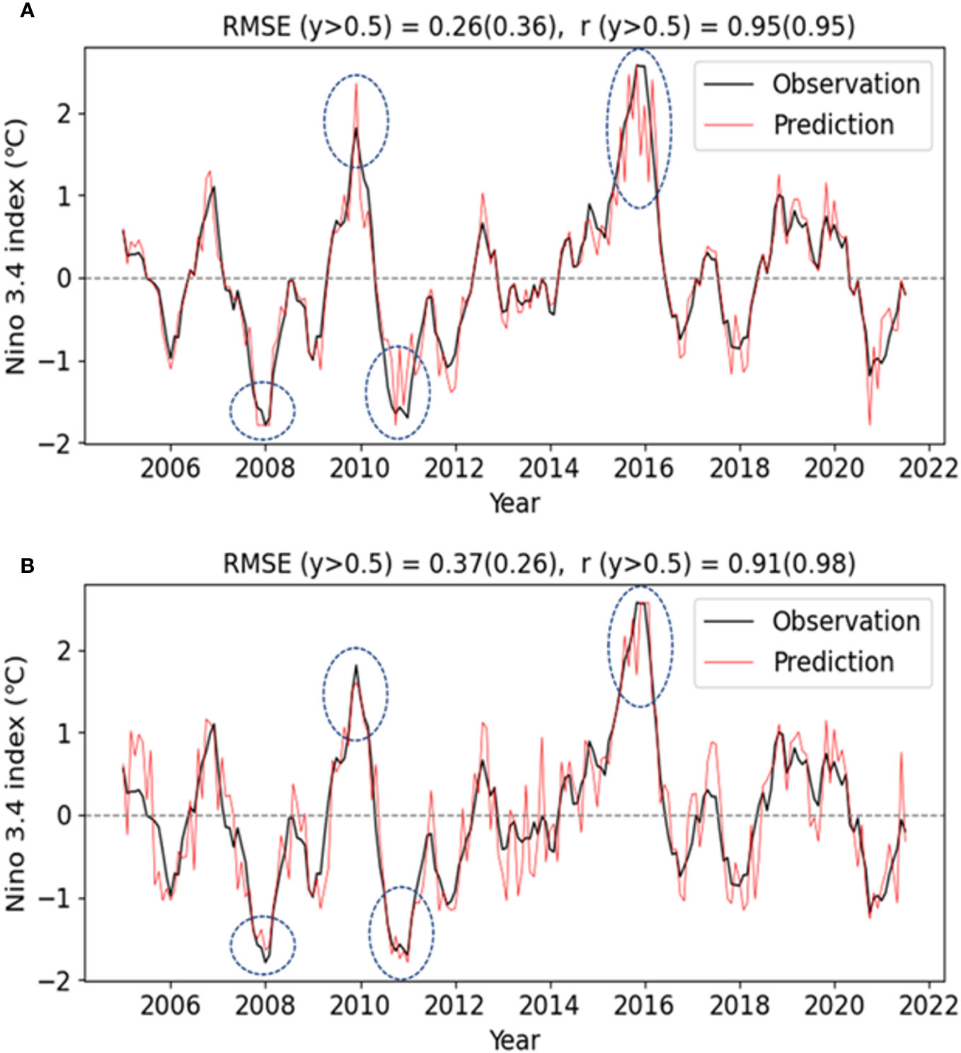
Figure 1 Two examples of the difference in the 6-month lead prediction performance of Niño3.4 (A) The case of high overall average predictive performance but relatively low prediction of abnormal years (y >0.5). (B) Low overall average predictive performance but relatively high prediction of abnormal years. Individual RMSEs and correlation skills (r), including the results for abnormal years only (y > 0.5, in parentheses), are shown at the top.

From a disaster prevention perspective, it is more important to better predict extreme ENSO years (i.e., El Niño and La Niña) than normal years (|Niño3.4|< 0.5°C). However, few studies have investigated models’ predictive performance focusing on abnormal ENSO years (|Niño3.4| > 0.5°C). Here, we propose a novel weighted loss function to improve prediction accuracy for abnormal years, which are much less frequent than normal years, but more important from the perspective of disasters. The method was applied to the LSTM neural network to predict Niño3.4. Predictive performance was evaluated for forecast lead times ranging from 1 to 12 months and compared with the results obtained using vanilla loss functions.

2 Methods

2.1 Neural network model

This study used the LSTM neural network, which has the advantage of long-term memory. LSTMs are specifically designed to address the challenge of long-term dependencies in time series data. They are capable of remembering information over extended periods, which is crucial for capturing patterns over extended time frames (Goodfellow et al., 2016). Traditional Recurrent Neural Networks (RNNs) often face the vanishing gradient problem, where gradients become too small for effective learning in deep networks. LSTMs mitigate this problem through their gating mechanisms. LSTMs are also highly flexible and can model the complexities of various time series data (Goodfellow et al., 2016), making them suitable for the diverse and dynamic nature of climate data.

For model training, time series of nine indices (Table 1) were used, in which the input data are monthly mean values for the 12 months prior to the base time, while the output data are the Niño3.4 index for 1–12 months after the base time. The model hyperparameters are shown in Table 2. In this study, Adam’s method (Kingma and Ba, 2014) was used as an optimizer, but L1 regularization, known as Lasso (Tibshirani, 1996), and L2 regularization, known as ridge regression (Hoerl and Kennard, 1970), which can prevent overfitting, were not used. This is because the use of L1 and L2 regularization can complicate the evaluation of the contribution of the loss function when interpreting the results, as the regularization effects can be mixed in (Hastie et al., 2004; Bishop, 2006). Instead of using regularization, we designed the neural network structure as simple as possible (i.e., the hidden size was set to 12) to prevent overfitting because the more complex the network configuration, the more it depends on the training data.

Table 1

Table 1 Indices used as input/output data for ENSO predictions.

Table 2

Table 2 Hyperparameters of the neural network model used in this study.

To improve prediction performance for abnormal ENSO years and ensure reliability, the optimized neural network model itself should first be constructed. Since the performance of artificial neural networks greatly depends on the quality and quantity of training data, the greatest possible volume of high-quality data was obtained, although it is more difficult to obtain sufficient data for training compared to other fields. If a model is designed as a complex network and has numerous parameters in the absence of sufficient data, performance improvement is limited due to overfitting. In general, when overfitting occurs, performance tends to be good during training but decreases significantly during testing. In this study, a neural network model optimized for small volumes of learning data was designed to prevent overfitting. RMSE and Pearson’s r were used to evaluate and compare the results of normal and abnormal years.

For the period January 1900–July 2021, for which nine input variables overlapped, the training period spanned 105 years, from January 1900 to December 2004, and the validation period covered about 18 years, from January 2005 to July 2022 (Figure 2). The last 12 years of data were reserved for the verification of the 12-month lead time prediction. Artificial intelligence models are generally developed by dividing the data into training, validation, and testing periods to increase the reliability of the results. However, the lack of long-term data for ENSO predictions makes it difficult to obtain data for testing. Moreover, since the main purpose of this study was to examine whether the prediction of abnormal ENSO years could be improved using a weighted loss function, we focused only examining the effect of the weighted loss function on training and validation. The validation period was set to about 18 years after 2005 to ensure that more than two strong El Niño and La Niña events were included. All input and output data were normalized using maximum and minimum normalization (MinMaxScaler) to make the dimension and size equal. Specifically, to reflect the characteristics of Niño3.4, the input data were normalized between 0 and 1, and the output was normalized between −1 and 1.

Figure 2

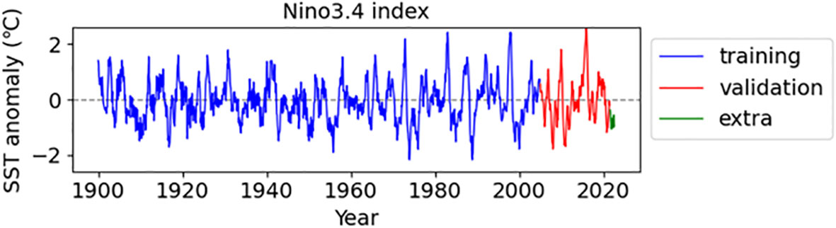
Figure 2 Niño3.4 time series used for training and validation. The extra data were used for the verification of the 12-month prediction.

Overfitting is a fundamental problem of machine learning that interferes with predictability. In general, overfitting occurs due to the presence of noise, the complexity of the neural network, and especially the limited size of training data. Ying (2019) suggested various methods, such as early stopping, network reduction, data expansion (data augmentation), and regularization, to prevent overfitting. Other methods have also been proposed, including dropout and regularization, small batches for training, low learning rates, simpler models (smaller capacity), and transfer learning (Koidan, 2019). This study used dropout, small batches, low learning rates, simpler models, and early stopping to prevent overfitting. The early stopping point was chosen to be when the validation loss was at its lowest value after the training loss had dropped sufficiently. Figure 3 is an example of training loss and validation loss plotted together. The relatively large total number of epochs was chosen so that many experiments would have enough time to learn about finding the best epoch for each experiment. For this experiment, we compared the prediction results at about 1100 epochs, the best value of validation.

Figure 3

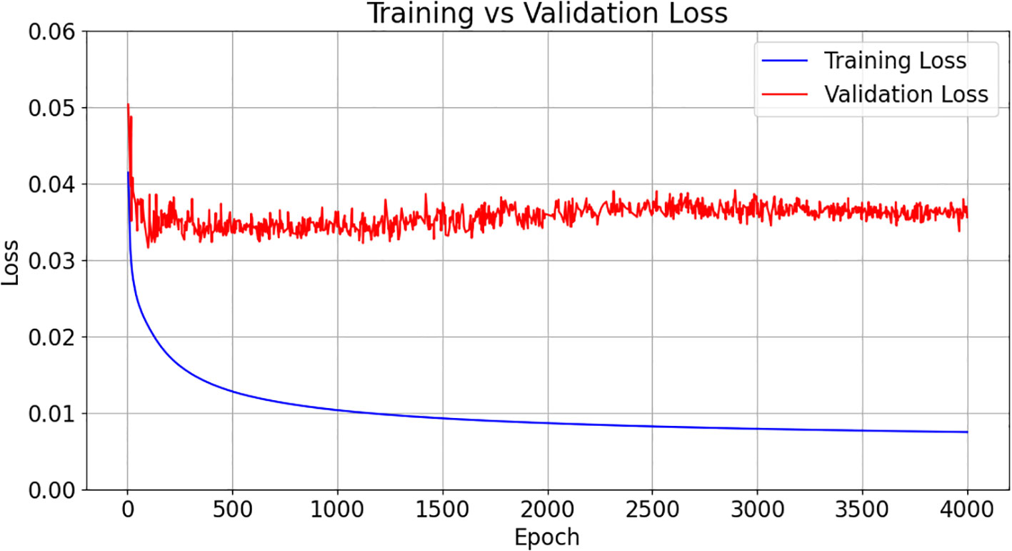
Figure 3 The loss curves of training and validation for the weighted L1 experiment (blue: training, red: validation). We analyzed the results at around 1100 epochs, which is the best value for validation after the training loss had dropped sufficiently.

2.2 Data

Monthly climate indices were downloaded from the official National Oceanic and Atmospheric Administration website (https://psl.noaa.gov/gcos_wgsp/Timeseries/; accessed Oct. 2022). Niño3.4 is the anomaly obtained by subtracting the climatological mean of the period 1981–2010 from the regional SST mean of 5°N–5°S and 170°W–120°W (Figure 4). Niño3.4 was used as a predictand, whereas the other indices (Table 1) were used as predictors. To find potential predictors, various climate indices that are related to ENSO, were selected based on literature research and during model training, the correlations between Niño3.4 and all potential ENSO-related indices were investigated. Finally, nine optimized predictors were then selected as input variables. Table 1 provides references explaining the relevance of each index to ENSO. Since the collected data pertained to different periods, only data for the period in which all variables overlapped were used.

Figure 4

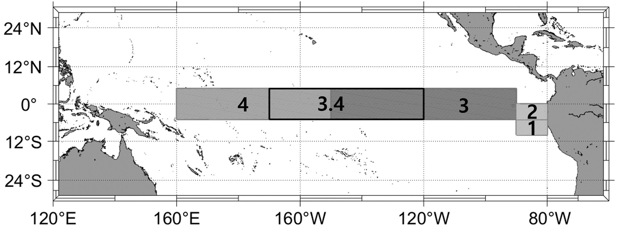
Figure 4 Definitions of various Niño indices.

2.3 Experimental methods and evaluation

Time series forecasting can be divided into univariate and multivariate forecasting, as well as one-step and multistep forecasting. Univariate forecasting uses one variable X for predictand Y, whereas multivariate forecasting uses multiple variables (X_s). One-step (many-to-one) forecasting predicts a simple future point (Y_t+n), while multistep (many-to-many) forecasting predicts multiple points (Y_t+1, Y_t+2,…, Y_t+n) simultaneously. This study used multivariate forecasting with nine input variables, allowing the use of as many observations and variables as possible. Multistep forecasting makes it possible to simultaneously make predictions for 1 to 12 months and maintain consistency between the prediction results for each lead time. One-step forecasting, which independently predicts each month, may perform well for specific individual forecasts but may not perform consistently across the entire lead times (Makridakis et al., 1998; Armstrong, 2001; Box et al., 2015). Figure 5 shows the schematic diagram illustrating input/output data and period for training and validation.

Figure 5

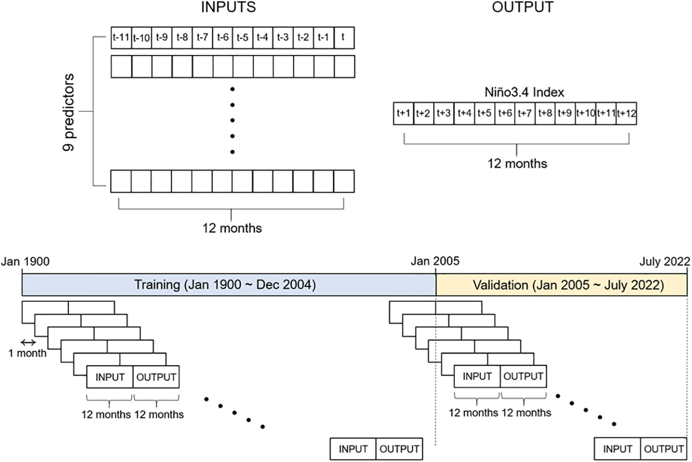
Figure 5 Schematic diagram illustrating input/output data and period for training and validation.

To consistently compare the experimental results, a random seed value in the neural network was fixed and tested (Madhyastha and Jain, 2019). We also did not use ensemble method because it combines multiple models to improve prediction performance, making interpretation more difficult compared to a single model (Hastie et al., 2004). This was a necessary step in the twin experiments conducted to investigate the performance of the loss functions. Table 2 shows the experimental configuration for the investigation of the Niño3.4 predictive performance using various weighted loss functions. A total of 4,000 epochs were trained for each experiment, and periodic verification was performed to select the best predictive performance. The procedure was similar to an early stopping method.

To evaluate the model’s accuracy and error simultaneously, the RMSE and Pearson’s r were compared between the predicted values and the Niño3.4 index. Both the RMSE and Pearson’s r had values between 0 and 1. The closer Pearson’s r is to 1, the higher the accuracy, and the closer the RMSE is to 0, the smaller the error. To investigate the performance of only abnormal years, the result of |Niño3.4| > 0.5°C was additionally presented.

3 Results

3.1 Design of weighted loss functions

In genal, three loss functions are used to calculate the loss of neural network models: L1 (mean absolute error; $L(y, f(x))=\left|(y-f(x))\right|$), L2 (mean squared error; $L(y, f(x))={(y-f(x))}^2$), and Huber (1964) ($L_{\delta }(y, f(x))=0.5{(y-f(x))}^2$ for $\left|y-f(x)\right|\le \delta$ and $\delta (\left|y-f(x)\right|-0.5\delta ,\text{ otherwise}$) where $L$ is the loss function, $y$ is the predictand, $f(x)$ is the predicted value, and δ is the boundary value separating quadratic and linear. L1 is less affected by outliers than the other two functions, and L2 is favorable for finding optimal values. Huber was developed to take advantage of L1 and L2 and compensate for their shortcomings based on the δ value and shows satisfactory learning ability in most neural networks because of its simplicity and good performance. In this study, these vanilla loss functions are multiplied by two (linear and quadratic) weight functions to weight loss value according to the level of the predictand. The right side of Figure 6 shows the two types of weight functions as an example—linear function (y) and quadratic function (y²), in which slopes of the functions are defined as 1, 5, and 10. This indicates that the weight increases linearly (or as a quadratic function) up to ±1.0, ± 0.2, and ±0.1, respectively. After that, the weight is fixed to 1 to be equal to the vanilla loss function. In this way, each loss value can be weighted according to the level of the predictand. This method can be expressed as follows:

Figure 6

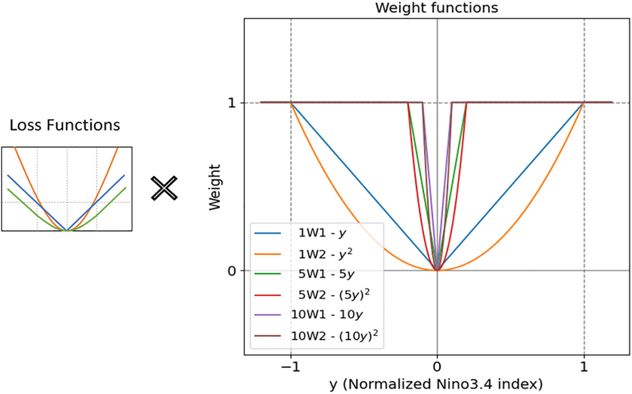
Figure 6 Schematic diagram explaining how to apply a weight function to a vanilla loss function. Here, linear (W1) and quadratic (W2) weight functions with slopes of 1, 5, and 10 are applied to the vanilla L1, L2, and Huber loss functions. The source code of the weighted loss function is provided in the Supplementary Information.

$$L_{\omega }(y, f(x))=L(y, f(x))\times W(y)$$

where $W(y)$ are the weight functions and are expressed as follows:

Linear (W1):

$$W(y)= \{\begin{array}{c}\mathbf{\text{slope}}\times \mathit{\text{y}} \mathbf{\text{for}} \mathit{\text{y}}\le \frac{\mathbf{1}}{\mathrm{slope}} ,\\ \mathbf{1} , \mathbf{\text{otherwise}}. \end{array}$$

Quadratic (W2):

$$W(y)= \{\begin{array}{c} {(\mathrm{slope}\times y)}^{\mathbf{2}} \mathbf{\text{for}} \mathit{\text{y}}\le \frac{\mathbf{1}}{\mathrm{slope}} ,\\ \mathbf{1} , \mathbf{\text{otherwise}}. \end{array}$$

Since the loss value is combined for all years and the model is trained to minimize this loss, reducing the weight of normal years using these equations allows for a greater focus on abnormal or extreme ENSO events. The adjusted weighting system ensures that the model does not underestimate significant abnormal events, improving prediction accuracy especially for extreme events. The optimal slope of the weighted functions was determined according to the distribution of the predictand (Niño3.4). In this study, six weighted functions, linear (W1) and quadratic (W2) functions with slopes of 1, 5, and 10, were tested based on the data distribution of Niño3.4 (Figure 7). For the period January 1900–July 2021, the training period spanned 105 years, from January 1900 to December 2004, and the validation period covered about 18 years, from January 2005 to July 2022.

Figure 7

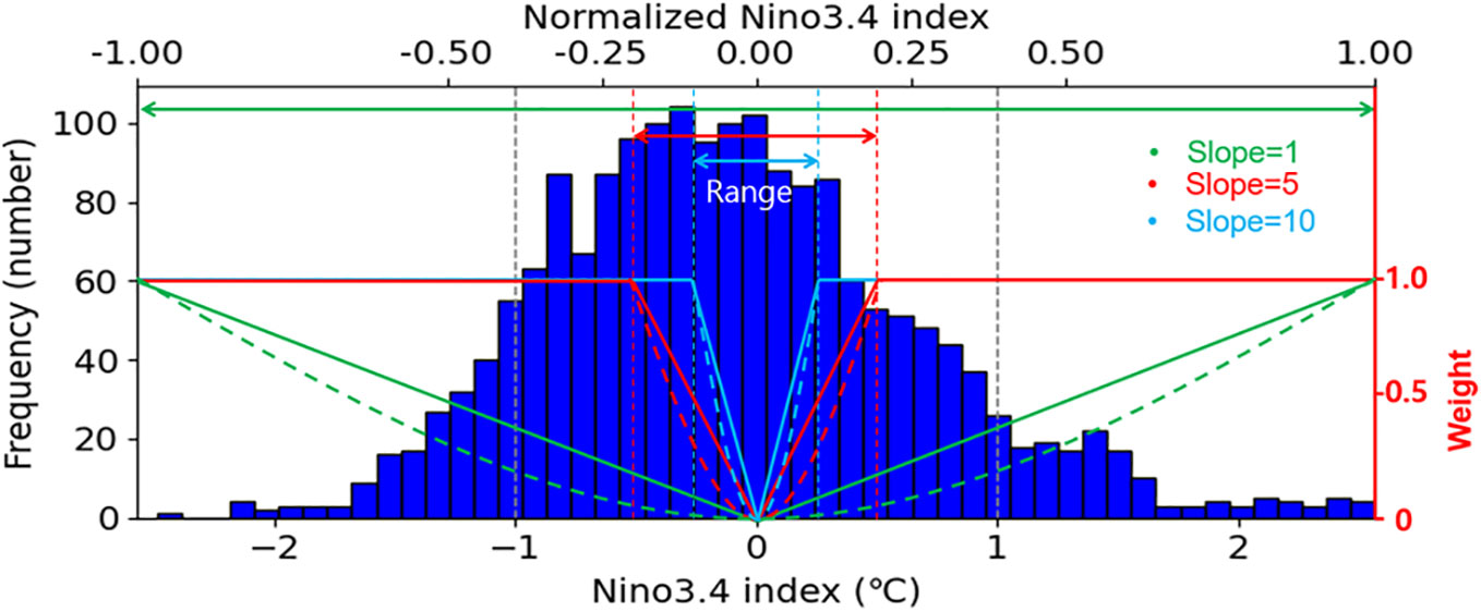
Figure 7 Histogram showing the distribution of Niño3.4 along with linear (W1) and quadratic (W2) weight functions with slopes of 1, 5, and 10. The bulk (81%) of the data were in the range of -1 to 1.

3.2 ENSO prediction results

A total of 18 experiments (Table 3) were performed by combining the six weight functions and the three vanilla loss functions (L1, L2, and Huber). Predictive performance was evaluated for lead times ranging from 1 to 12 months. In each case, the results obtained using the vanilla L1, L2, and Huber loss functions were compared to those obtained using the weight functions. The weight functions that performed best for the three loss functions are shown in Table 4.

Table 3

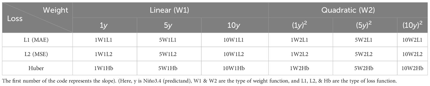
Table 3 Experimental configuration of the weighted loss functions to investigate Niño3.4 prediction performance.

Table 4

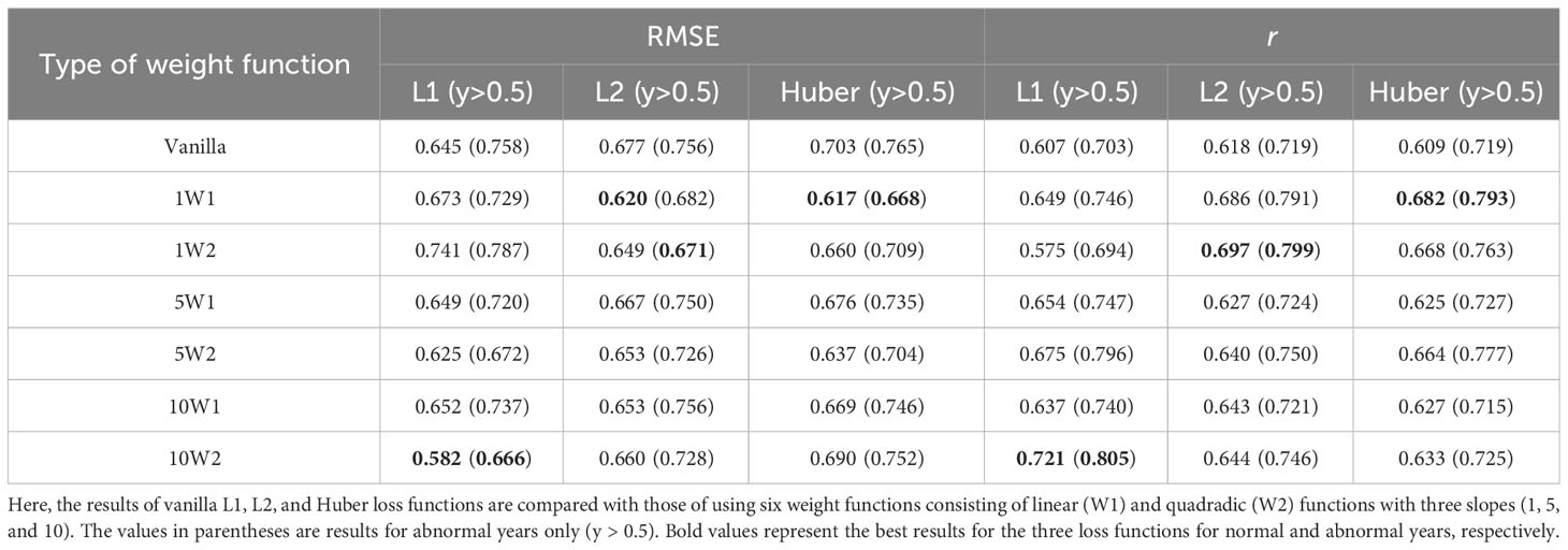
Table 4 Averaged all-season RMSE and correlation skills of Niño3.4 for all-lead forecast times for the validation period (2005–2022).

Figure 8 shows a comparison of the Niño3.4 predictions for abnormal years (y>0.5°C) over lead times ranging from 1 to 12 months using the vanilla loss function and the six weighted loss functions. For L1, most of weighted functions outperformed vanilla function on average in abnormal years (Figures 8A, B; Table 4). In particular, the performance improvement was greater for longer lead predictions. For the L1 loss function, a quadratic weight function with a slope of 10 (10W2; purple line) performed best, followed by 5W2 (Table 4). For the L2 loss functions, all weight functions had lower errors and higher correlations than vanilla L2 (Figures 8C, D; Table 4). For L2, a quadratic weight function with a slope of 1 (1W2; dark yellow line) showed the best performance with a 10-20% improvement over vanilla L2 in the 6–12-month predictions of abnormal years. However, the performance improvement of the best (optimal) weighted loss function (i.e., 1W2) was smaller than that of L1. This is because vanilla L2 is known to have significantly better performance compared to L1 (also shown in our results; compare the black lines in Figures 8A–D), making further improvement by the weighted loss function difficult. For the Huber loss functions, the results were overall similar to L2, except that the best performing model was a linear weighted function with a slope of 1 (1W1, green line Figures 8E, F; Table 4). In particular, 1W1 showed the largest improvement over vanilla Huber functions in the 6–9-month lead predictions (Figures 8E, F). Analysis of extremely abnormal years with the Niño3.4 index anomalies above 1.0 °C (y>1.0) was also consistent with results from abnormal years with a threshold of 0.5°C (Figure 9). That is, the weighted loss function performs better than the vanilla loss function, and the best weighted loss functions for L1 and L2 were 10W2 and 1W2, respectively.

Figure 8

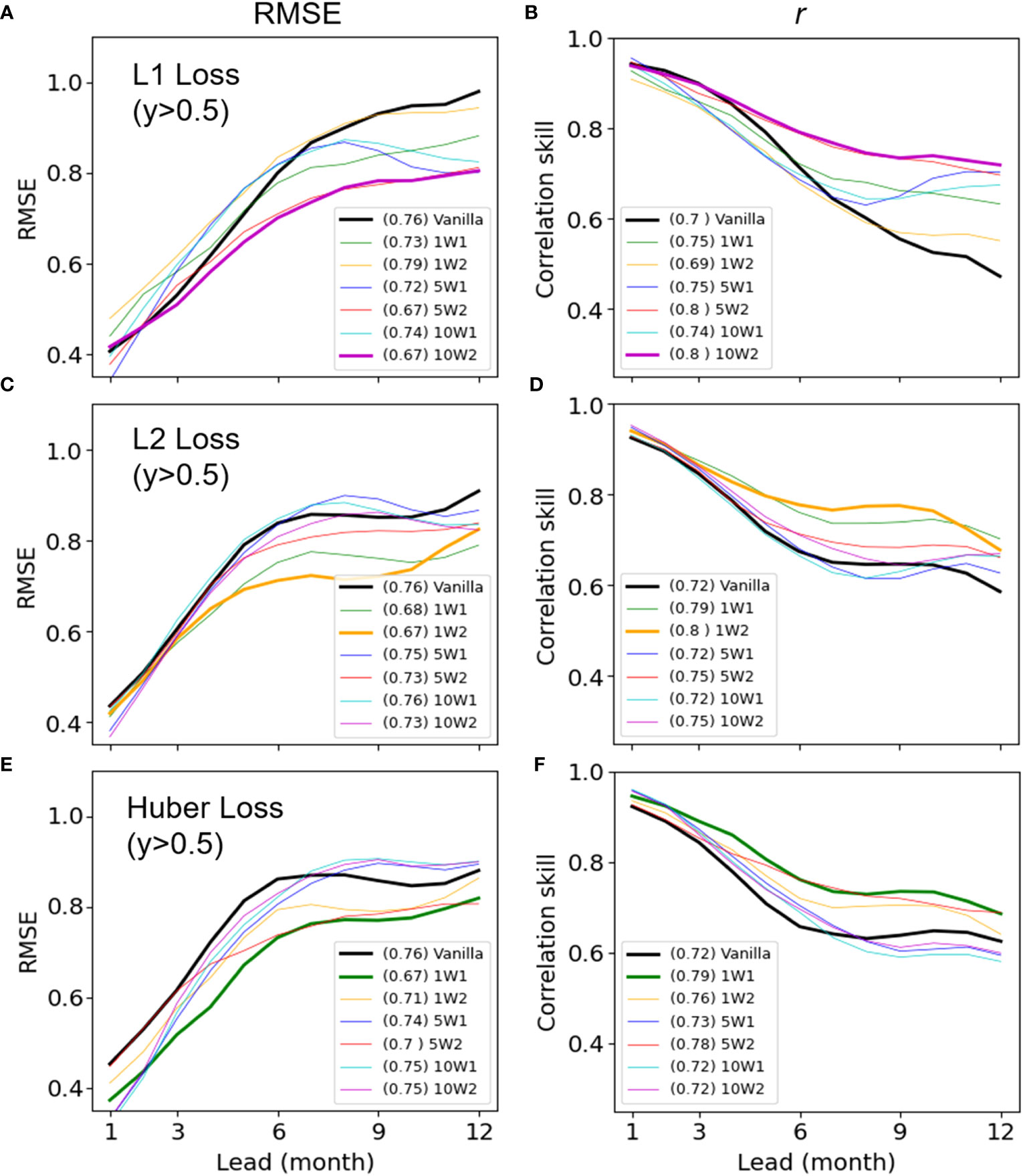
Figure 8 Comparisons of the all-season RMSEs and correlation skills of Niño3.4 for abnormal years (y>0.5°C) as functions of forecast lead times. For L1 (A, B), L2 (C, D), and Huber (E, F), comparisons were made using vanilla and six weighted loss functions over the validation period (2005–2022) and the best results for each were shown as bold colored lines.

Figure 9

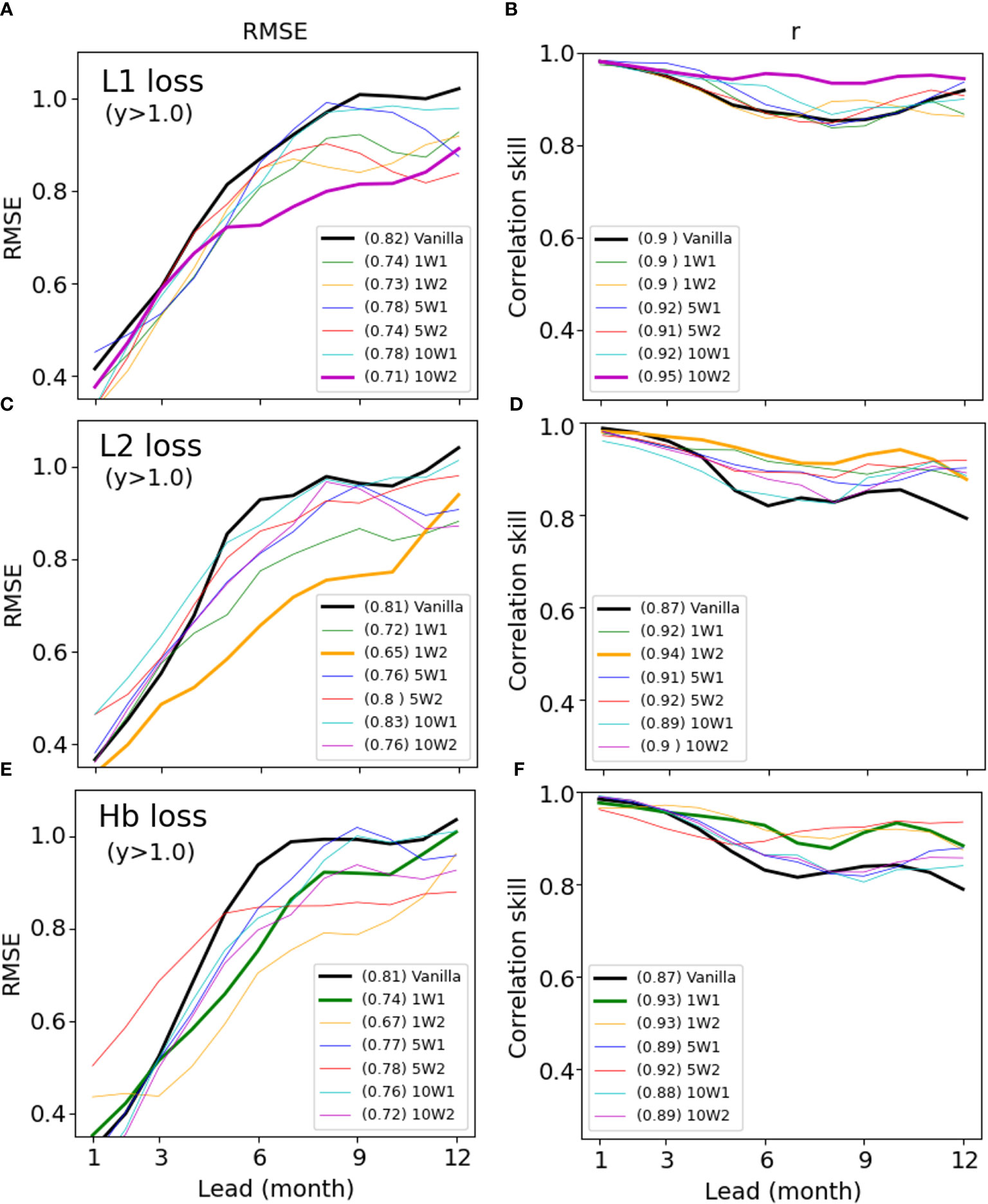
Figure 9 Same as Figure 8 but for extremely abnormal years (y>1.0°C) for L1 (A, B), L2 (C, D), and Huber (E, F).

ENSO predictive performance over six-month lead times is a widely used metric when evaluating models. Previous models have shown remarkable performance for up to 6-month lead times (e.g., Ham et al., 2019; Yan et al., 2020). In this study, the best model (10W2L1) for 6-month lead predictions had an RMSE of 0.61 and a correlation skill of 0.71 for all years, which is comparable to the performance of previous state-of-the-art studies (Figure 10). The high performance is mainly the result of a significant improvement (i.e., from 0.8 to 0.70 for RMSE and 0.71 to 0.79 for correlation skill) over the vanilla loss function in abnormal years. In particular, the use of the weighted loss function significantly improved the performance of strong El Niño in 2015–2016 and strong La Niña in 2007–2008 and 2010–2011. For the latest period, however, the performance was relatively poor (Figure 10). This could be due to changes in climate behavior or the evolution of factors influencing ENSO in recent years (Cai et al., 2023), and possibly because the model did not take these into account.

Figure 10

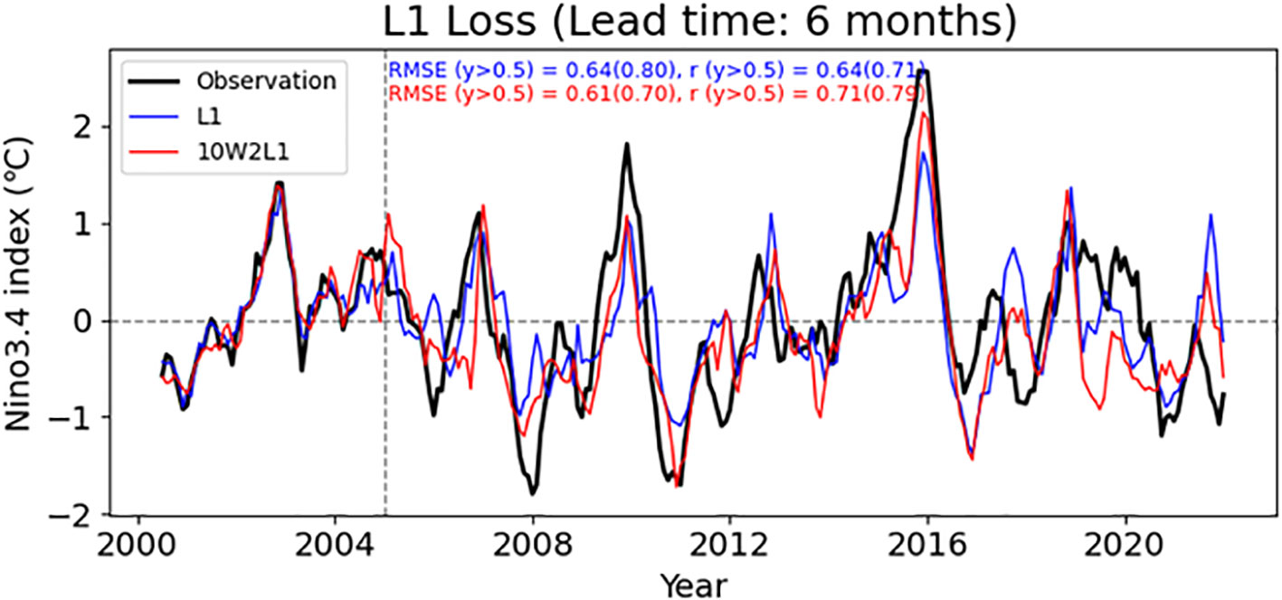
Figure 10 6-month lead predictions for Niño3.4 using the vanilla L1 loss function (blue line) and an optimal weighted loss function (10W2L1, red line). The observed Niño3.4 is also shown (black line). Individual RMSEs and correlation skills for the validation period (2005–2022), including the results for abnormal years only (y > 0.5, in parentheses), are shown at the top. An additional time series from 2000 to 2004, the last part of the training period, is shown here to ensure that there is no overfitting.

4 Discussion

The optimal slope of the weight functions was determined depending on the combination of the distribution of the y data and the function used. Therefore, the selection of the slope also requires an optimization process similar to the tuning of hyperparameters. In this study, we conducted more experiments than those presented here, but only the results of three discrete slopes (1, 5, 10) are shown here. This is because we believe that the impact of using a weighted loss function in this study can be sufficiently explained through the three samples. The experimental results show that the smaller the slope, the smaller the error in most cases of abnormal years (Figure 11). This may be because the frequency of the y data generally decreases almost linearly or quadratic with y (Figure 7). A closer look reveals that slope 1 generally shows the best performance except quadratic-L1 (Figure 11). When the slope was further reduced to 0.5, the performance was similar to that of slope 1 (not shown). In the case of quadratic-L1, slope 5 or 10 showed the best performance. The distribution of the y data shows that the bulk (81%) of the data were in the range of −1 to 1 and the ranges of slopes 5 and 10 correspond to where the data is concentrated (Figure 7). In some cases, therefore, the greatest benefit can be achieved by reducing the weights only in this high frequency range. These results emphasize again that the optimal type of weight function and slope should be determined according to the data distribution.

Figure 11

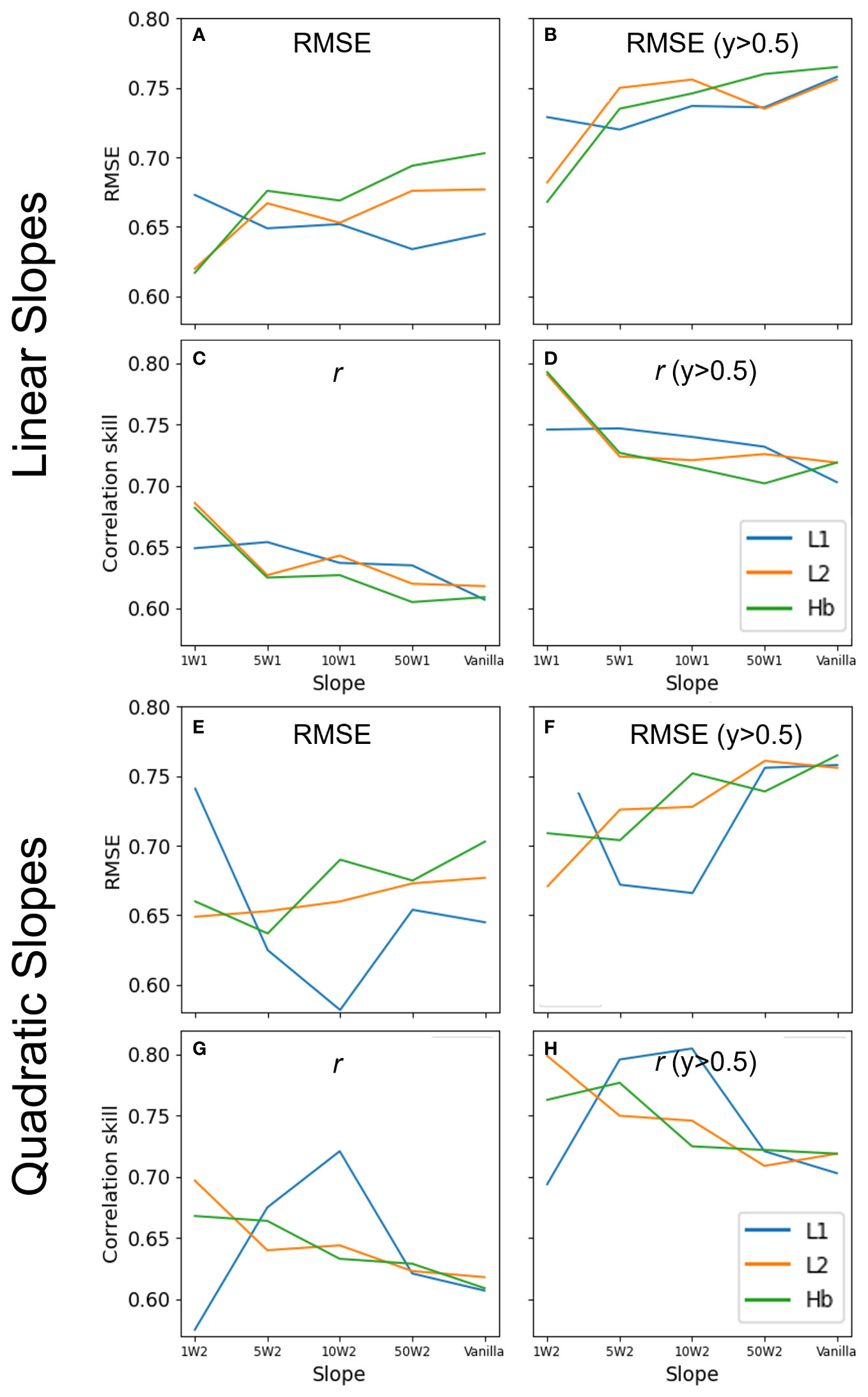
Figure 11 RMSEs and correlation skills of linear (A–D) and quadratic (E–H) weight function according to the slope. The performance of the weight function generally improves as the slope decreases, but the quadratic function for L1 performs best at slopes of 5 and 10. The results for abnormal years only (y > 0.5) are shown in (B, D, F, H).

In this study, only simple linear and quadratic functions were tested for sensitivity, but it is possible to develop and use various weighting functions (including known probability distribution functions) that better express the distribution of data. The current method is similar to data augmentation and batch sampling in that it solves the data imbalance problem, but it has the advantage of using all the data without artificially reducing or increasing the sample and using various weighting functions to focus on and optimize the desired target.

Observational data necessary for the development of ENSO prediction models using artificial neural networks are insufficient. To solve this problem, Ham et al. (2019) devised a transfer learning method using the results of a three-dimensional global circulation model. Initially, we also constructed an LSTM model using additional long-term climate model data, and tested their performance. However, the uses of these data did not significantly improve the model’s predictive accuracy. This may be because the numerical model itself has limitations in realistically simulating ENSO and this can negatively affect learning ability in current LSTM experiments. Subsurface ocean information, known as an early origin of ENSO variations, was also not used as a potential predictor in this study, as there is no long-term subsurface data with high accuracy, and the LSTM’s test results did not show a significant improvement in performance. In fact, we have tested subsurface variables extracted from the three-dimensional ocean data of Simple Ocean Data Assimilation (SODA), such as mixed layer depth and thermocline slope, as potential predictors, but did not achieve any significant performance improvement. This may be because that subsurface ocean data has lower accuracy and shorter duration compared to SST data, due to the difficulty in obtaining observational data, which may have contributed to the lack of performance improvement.

While many recent studies have focused on improving ENSO forecasting at long lead times (>1.5 years 18 months) (Luo et al., 2008; Doi et al., 2016; Ham et al., 2019; Patil et al., 2023), this study aims to improve accuracy and reliability for extreme or abnormal ENSO events using a new weighted loss function. We believe that the analysis results presented here, based on a lead time of up to one year, can support the claims and conclusions of this study. However, it is meaningful to investigate whether the current method accurately predicts extreme/abnormal ENSO events even with such long lead times. This remains a task for future research.

State-of-the-art ENSO prediction models can be developed using better methods and data, but it is important that this study can contribute to further improving the performance of these artificial intelligence models. In particular, the method based on the weighted loss functions presented herein can be effectively used when the observational data for training are insufficient and when the number of extreme events is small. Given that most extreme events are infrequent, the proposed method can be used to predict not only extreme ENSO but also various other extreme weather and climate events such as tropical cyclone, floods, drought, and heat waves.

This study does not explain which predictors contribute the most to the improvement in accuracy for the abnormal years since AI models are composed of non-linear relationships between predictors, which makes them difficult to interpret. In the case of CNN, heatmaps are often used as a basis for judging the results, but even this does not explain the contribution of the predictors. The field of Explainable AI (XAI) and Causal Inference is developing to study which factors a model has chosen as important and this is an area we are interested in exploring in future research.

Data availability statement

The raw data supporting the conclusions of this article will be made available by the authors, without undue reservation.

Author contributions

DK: Writing – original draft, Conceptualization, Data curation, Investigation, Methodology. IM: Writing – review & editing, Funding acquisition, Investigation, Supervision. CL: Writing – review & editing, Methodology, Validation. SW: Writing – review & editing, Funding acquisition, Validation.

Funding

The author(s) declare financial support was received for the research, authorship, and/or publication of this article. This work was supported by Institute of Information & Communications Technology Planning & Evaluation (IITP) grant funded by the Korea government (MSIT) [RS-2022-00155915, Artificial Intelligence Convergence Innovation Human Resources Development (Inha University)], Korea Institute of Marine Science & Technology Promotion (KIMST) funded by the Ministry of Oceans and Fisheries, Korea (20220051 Gyeonggi-Incheon SeaGrant), and the National Research Foundation of Korea (NRF) grant funded by the Korea government(MSIT) (No. RS-2022-00144325).

Conflict of interest

The authors declare that the research was conducted in the absence of any commercial or financial relationships that could be construed as a potential conflict of interest.

The author(s) declared that they were an editorial board member of Frontiers, at the time of submission. This had no impact on the peer review process and the final decision.

Publisher’s note

All claims expressed in this article are solely those of the authors and do not necessarily represent those of their affiliated organizations, or those of the publisher, the editors and the reviewers. Any product that may be evaluated in this article, or claim that may be made by its manufacturer, is not guaranteed or endorsed by the publisher.

References

An S.-I., Jin F.-F. (2004). Nonlinearity and asymmetry of ENSO. J. Clim. 17, 2399–2412. doi: 10.1175/1520-0442(2004)017<2399:NAAOE>2.0.CO;2

CrossRef Full Text | Google Scholar

Armstrong J. S. (2001). Principles of forecasting: A handbook for researchers and practitioners (Norwell: Kluwer Academic Publishers), 849.

Google Scholar

Ashok K., Guan Z., Yamagata T. (2003). A look at the relationship between the ENSO and the Indian Ocean Dipole. J. Meteor. Soc Japan 81, 41–56. doi: 10.2151/jmsj.81.41

CrossRef Full Text | Google Scholar

Barnston A. G., Chelliah M., Goldenberg S. B. (1997). Documentation of a highly ENSO-related SST region in the equatorial Pacific. Atmos.-Ocean 35, 367–383. doi: 10.1080/07055900.1997.9649597

CrossRef Full Text | Google Scholar

Barnston A. G., Tippett M. K., L'Heureux M. L., Li S., Dewitt D. G. (2012). Skill of real-time seasonal ENSO model predictions during 2002–11: Is our capability increasing? Bull. Am. Meterol. Soc 93 (5), 631–651. doi: 10.1175/BAMS-D-11-00111.1

CrossRef Full Text | Google Scholar

Bishop C. M. (2006). Pattern recognition and machine learning, Edition: View all formats and editions (New York: Springer).

Google Scholar

Box G. E., Jenkins G. M., Reinsel G. C., Ljung G. M. (2015). Time series analysis: Forecasting and control (Hoboken: John Wiley & Sons).

Google Scholar

Cachay S. R., Erickson E., Bucker A. F. C., Pokropek E., Potosnak W., Osei S. (2021). Graph neural networks for improved El Niño forecasting. Tackling climate change with machine learning workshop at NeurIPS 2020 (Neural Information Processing Systems Foundation). Available at: https://arxiv.org/pdf/2012.01598.pdf.

Google Scholar

Cai W., Ng B., Geng T., et al (2023). Anthropogenic impacts on twentieth-century ENSO variability changes. Nat. Rev. Earth Environ. 4, 1–12. doi: 10.1038/s43017-023-00427-8

CrossRef Full Text | Google Scholar

Cal W., Wu L., Lengaigne M., Li T., Mcgregor S., Kug. J. S. (2019). Pantropical climate interactions. Science 363 (6430), eaav4236. doi: 10.1126/SCIENCE.AAV4236

PubMed Abstract | CrossRef Full Text | Google Scholar

Cho K., van Merrienboer B., Gulcehre C., Bahdanau D., Bougares F., Schwenk H. (2014). Learning phrase representations using RNN encoder-decoder for statistical machine translation. arXiv. doi: 10.3115/v1/D14-1179

CrossRef Full Text | Google Scholar

Dijkstra H. A., Petersik P., Garcia E. H., Lopez C. (2019). The application of machine learning techniques to improve El Niño prediction skill. Front. Phys. 7. doi: 10.3389/fphy.2019.00153

CrossRef Full Text | Google Scholar

Doi T., Behera S. K., Yamagata T. (2016). Improved seasonal prediction using the S INTEX-F2 coupled model. J. Adv. Model. Earth Syst. 8 (4), 1847–1867. doi: 10.1002/2016MS000744

CrossRef Full Text | Google Scholar

Elman J. L. (1990). Finding structure in time. Cogn. Sci. 14, 179–211. doi: 10.1016/0364-0213(90)90002-E

CrossRef Full Text | Google Scholar

Gers F. A., Schmidhuber J., Cummins F. (2000). Learning to forget: Continual prediction with LSTM. Neural Comput. 12, 2451–2471. doi: 10.1162/089976600300015015

PubMed Abstract | CrossRef Full Text | Google Scholar

Goodfellow I., Bengio Y., Courville A. (2016). Deep Learning (Adaptive Computation and Machine Learning series) (Cambridge, MA: The MIT Pres).

Google Scholar

Graves A. (2012). Long short-term memory. Neural Comput. 9, 37–45. doi: 10.1007/978-3-642-24797-2_4

CrossRef Full Text | Google Scholar

Gupta M., Kodamana H., Sandeep S. (2020). Prediction of ENSO beyond spring predictability barrier using deep convolutional LSTM networks. IEEE Geosci. Remote. Sens. Lett. 19, 1–5. doi: 10.1109/LGRS.2020.3032353

CrossRef Full Text | Google Scholar

Ham Y. G., Kim J. H., Luo J. J. (2019). Deep learning for multi-year ENSO forecasts. Nature 573, 568–1572. doi: 10.1038/s41586-019-1559-7

PubMed Abstract | CrossRef Full Text | Google Scholar

Han Y. G., Kug J. S. (2012). How well do current climate models simulate two types of El Niño? Clim. Dyn. 39, 383–398. doi: 10.1093/nsr/nwy105

CrossRef Full Text | Google Scholar

Hassanibesheli F., Kurths J., Boers N. (2022). Long-term ENSO prediction with echo-state networks. Env. Res. 1 (1), 011002. doi: 10.1088/2752-5295/ac7f4c

CrossRef Full Text | Google Scholar

Hastie T., Tibshirani R., Friedman J. H. (2004). The elements of statistical learning: data mining, inference, and prediction. Math. Intelligencer 27 (2), 83–85. doi: 10.1007/BF02985802

CrossRef Full Text | Google Scholar

He D., Lin P., Liu H., Ding L., Jiang J. (2019). DLENSO: A deep learning ENSO forecasting model. PRICAI 2019: Trends Artif. Intell. 12–23. doi: 10.1007/978-3-030-29911-8_2

CrossRef Full Text | Google Scholar

Hoerl A. E., Kennard R. W. (1970). Ridge regression: Biased estimation for nonorthogonal problems. Technometrics 12, 55–67. doi: 10.1080/00401706.1970.10488634

CrossRef Full Text | Google Scholar

Huber P. J. (1964). Robust estimation of a location parameter. Ann. Math. Stat. 35, 73–101. doi: 10.1214/aoms/1177703732

CrossRef Full Text | Google Scholar

Kingma D. P., Ba J. (2014). Adam: A method for stochastic optimization. arXiv preprint arXiv:1412.6980.

Google Scholar

Koidan K. (2019). 7 effective ways to deal with a small dataset (Edwards, Colorado 81632, USA: HackerNoon). Available at: https://hackernoon.com/7-effective-ways-to-deal-with-a-small-dataset-2gyl407s.

Google Scholar

Kug J. S., Jin. F. F., An. S. I. (2009). Two types of El Niño events: Cold tongue El Niño and warm pool El Niño. J. Climate 22, 1499–1515. doi: 10.1175/2008JCLI2624.1

CrossRef Full Text | Google Scholar

Luo J. J., Masson S., Behera S. K., Yamagata T. (2008). Extended ENSO predictions using a fully coupled ocean–atmosphere model. J. Climate 21 (1), 84–93. doi: 10.1175/2007JCLI1412.1

CrossRef Full Text | Google Scholar

Madhyastha P., Jain R. (2019). On model stability as a function of random seed. arXiv preprint arXiv:1909.10447.

Google Scholar

Makridakis S., Wheelwright S. C., Hyndman R. J. (1998). Forecasting: methods and applications. J. Am. Stat. Assoc. 94, (445). doi: 10.2307/2287014

CrossRef Full Text | Google Scholar

Newman M., Alexander M. A., Ault T. R., Cobb K. M., Deser C., Di Lorenzo E., et al. (2016). The pacific decadal oscillation, revisited. J. Climate 29, 4399–4427. doi: 10.1175/JCLI-D-15-0508.1

CrossRef Full Text | Google Scholar

Patil K. R., Jayanthi V. R., Behera S. (2023). Deep learning for skillful long-lead ENSO forecasts. Front. Clim. 4, 1058677. doi: 10.3389/fclim.2022.1058677

CrossRef Full Text | Google Scholar

Shi Y., Su J. (2020). A new equatorial oscillation index for better describing ENSO and westerly wind bursts. J. Meteorol. Res. 34, 1025–1037. doi: 10.1007/s13351-020-9195-6

CrossRef Full Text | Google Scholar

Soulard N., Lin H., Yu B. (2019). The changing relationship between ENSO and its extratropical response patterns. Sci. Rep. 9, 6507. doi: 10.1038/s41598-019-42922-3

PubMed Abstract | CrossRef Full Text | Google Scholar

Tang Y., Zhang R. H., Liu T., Duan W., Yang D., Zheng F. (2018). Progress in ENSO prediction and predictability study. Natl. Sci. Rev. 5, 826–839. doi: 10.1126/SCIENCE.AAV4236

CrossRef Full Text | Google Scholar

Tibshirani R. (1996). Regression shrinkage and selection via the lasso. J. R. Stat. Society: Ser. B (Methodological) 58, 267–288. doi: 10.1111/j.2517-6161.1996.tb02080.x

CrossRef Full Text | Google Scholar

Timmermann A., An S. I., Kug J. S., Jin F. F., Cai W., Capotondi A. (2018). El niño–southern oscillation complexity. Nature 559, 535–545. doi: 10.1038/S41586-018-0252-6

PubMed Abstract | CrossRef Full Text | Google Scholar

Wang B. (1995). Interdecadal changes in El Niño onset in the last four decades. J. Clim. 8, 267–285. doi: 10.1175/1520-0442(1995)008<0267:icieno>2.0.co;2

CrossRef Full Text | Google Scholar

Wang C. (2018). A review of ENSO theories. Natl. Sci. Rev. 5 (6), 813–825. doi: 10.1093/nsr/nwy104

CrossRef Full Text | Google Scholar

Xiaoqun C., Yanan G., Bainian L., Kecheng P., Guangjie W., Mei G. (2020). ENSO prediction based on Long Short-Term Memory (LSTM). IOP Conf. Ser.: Mater. Sci. Eng. 799, (1), 012035. doi: 10.1088/1757-899X/799/1/012035

CrossRef Full Text | Google Scholar

Yan J., Mu L., Wang L., Ranjan R., Zomaya A. Y. (2020). Temporal convolutional networks for the advance prediction of ENSO. Sci. Rep. 10 (1), 8055. doi: 10.1038/s41598-020-65070-5

PubMed Abstract | CrossRef Full Text | Google Scholar

Yang Y., Dong J., Sun X., Lima E., Mu Q., Wang X. (2018). A CFCC-LSTM model for sea surface temperature prediction. IEEE Geosci. Remote. Sens. 15, 207–211. doi: 10.1109/lgrs.2017.2780843

CrossRef Full Text | Google Scholar

Yeh S. W., Kug J. S., Dewitte B., Kwon M. H., Kirtman B. P., Jin F. F. (2009). El Niño in a changing climate. Nature 461, 511–514. doi: 10.1038/nature08316

PubMed Abstract | CrossRef Full Text | Google Scholar

Ying X. (2019). An overview of overfitting and its solutions. J. Phys.: Conf. Ser. 1168, 022022. doi: 10.1016/j.newast.2016.09.004

CrossRef Full Text | Google Scholar

Zhang W., Mei X., Geng X., Turner A. G., Jin F.-F. (2019). A nonstationary ENSO–NAO relationship due to AMO modulation. J. Climate 32 (1), 33–43. doi: 10.1109/lgrs.2017.2733548

CrossRef Full Text | Google Scholar