 Chengzhi Lu
 Fan Zhang
 Jianjun Jia
 Ya Ping Wang
- 1State Key Laboratory of Estuarine and Coastal Research, Institute of Eco-Chongming, East China Normal University, Shanghai, China
- 2Southern Marine Science and Engineering Guangdong Laboratory (Zhuhai), Zhuhai, China
- 3Key Laboratory of MEA, Ministry of Education, East China Normal University, Shanghai, China
With sea level rise (SLR), tidal nuisance flooding has become a growing threat, especially around estuaries with large tidal amplitudes. This study investigated how sea level change affects tides in Hangzhou Bay, a macro-tidal estuary with high SLR rate. By downscaling climate projections to a regional hydrodynamic model, the amplitude of primary tidal constituent (M2) was predicted to increase by 0.25 m in the upper bay, where the amplitude of major diurnal tide (K1) was also predicted to increase by 15%. In addition, the sensitivity of tidal amplitude to mean sea level was examined by a set of numerical simulations with different SLR. It was found that the increase of tidal amplitude is nonlinear to SLR, and the tidal amplitudes almost cease to increase when SLR is over 1.5 m. Although predictions show less amplitude changes in the lower bay, Zhoushan Archipelago around the bay mouth strongly modulates the incoming tidal energy, thus affecting the tidal amplitude in the upper bay. Energy budget analysis revealed that the complex topography, such as narrow channels, in the archipelago area leads to strong horizontal shear, which dissipates approximately 25% of total tidal energy in the bay. On the other hand, around 60% of the energy is dissipated in the bottom boundary layer. However, the bottom dissipation decreases by 4% due to reduced friction, while horizontal dissipation increases by 10% due to enhanced horizontal shear with SLR. This suggests that the strong horizontal shear in the Zhoushan archipelago region can play a more important role in the tidal energy budget in the future.
1 Introduction
Sea level rise (SLR) is a global phenomenon that has garnered significant attention. Analysis of historical data from tidal gauge stations reveals that the global sea level has been rising at a rate of 1.2 ± 0.2 mm yr-1 from 1900 to 1990 and 3.0 ± 0.7 mm yr-1 from 1993 to 2010 (Hay et al., 2015). The Sixth Assessment Report of the Intergovernmental Panel on Climate Change (IPCC AR6) predicts that the global mean sea level will increase by 0.38-0.77 m from 1995-2014 to 2100 (Fox-Kemper et al., 2021). However, coastal areas may experience higher rates of relative SLR due to factors such as glacial isostatic adjustment (Peltier, 1999), groundwater depletion (Konikow, 2011), sediment compaction (Edwards, 2006; Horton and Shennan, 2009), and changes in nearshore sea level gradients caused by variations in ocean current strength (Ezer, 2013; Ezer et al., 2013). For instance, in Hangzhou Bay, the mean sea level has been increasing at a rate of 4.6 mm yr-1 between 1978 and 2017, which is 1.5 times higher than the average SLR rate in China seas (3.3 mm yr-1) (Kuang et al., 2017); and the highest local SLR rate reached 11 mm yr-1 (Feng et al., 2018). Such high local SLR rate is closely related to the fast land subsidence rate (up to 2 mm yr-1) in this region (Wang et al., 2012).
Rapid coastal SLR can have significant implications, including increased frequency of nuisance flooding under normal weather conditions and more severe coastal inundation during storm surge events (Taherkhani et al., 2020). The frequency of nuisance flooding and the level of storm surge are closely linked to changing tides (Horsburgh and Wilson, 2007). SLR alters water depth and reshapes the coastline, which in turn affects the energy dissipation and resonance behavior of tidal waves (Zhong et al., 2008). The response of tides to SLR has been an active area of research in recent decades (Holleman and Stacey, 2014; Lee et al., 2017; Feng et al., 2019). On the Yellow Sea shelf, tidal amplitude decreases in the north but increases in the south (Feng et al., 2019). Similarly, with a 2 m SLR, Liaodong Bay and the eastern part of Bohai Bay experience increased tidal amplitude, while Laizhou Bay in the south experiences decreased tidal amplitude (Pelling et al., 2013). On the European continental shelf, the M2 constituent is particularly sensitive in resonant areas, leading to significant amplitude decreases or increases (Pickering et al., 2012). In Chesapeake Bay and Delaware Bay, Lee et al. (2017) found that the impact of SLR on tidal range is influenced by coastal management strategies. Specifically, the construction of a hypothetical seawall along the current shoreline to prevent flooding of low-lying areas led to an increase in tidal range. Additionally, Ross et al. (2017) found that the response of tides to SLR is nonlinear. Their model indicated that the sensitivity of M2 amplitude to SLR is higher in the upper reach of Chesapeake Bay compared to the lower bay. These studies highlight the complex and varied response of tidal amplitudes to SLR, emphasizing the need for region-specific investigations in different coastal areas.
It is worth noting that funnel-shaped estuaries, such as Hangzhou Bay, experience more significant changes in tides compared to the open coast with SLR (Passeri et al., 2015; Kuang et al., 2017; Haigh et al., 2020; Khojasteh et al., 2020). Hangzhou Bay is a funnel-shaped estuary connecting the Qiantang River and the East China Sea. The width of the bay decreases rapidly from approximately 100 km in the lower bay to less than 20 km in the upper bay over 100 km distance. Consequently, the maximum tidal range in the upper bay reaches 9 m. The coastline of Hangzhou Bay has undergone significant changes in recent decades due to natural siltation and land reclamation, which have had a notable impact on the hydrodynamics of the region. Ji et al. (2015) suggest that tidal amplitude within narrow channels of the archipelago region is not sensitive to island reclamation, but the tidal current velocity experiences substantial reduction.
The behavior of tidal waves in funnel-shaped estuaries is influenced by various factors, including shoreline narrowing, bottom friction, water depth shallowing, and partial reflection of tidal waves at the bay head (Savenije et al., 2008; Toffolon and Savenije, 2011; Van Rijn, 2011). In the case of Hangzhou Bay, the tidal waves are not only affected by these factors but also by Zhoushan Archipelago, a group of islands of different sizes and shapes located at the eastern connection with the East China Sea. This adds complexity to the tidal response to SLR in this region. The coastlines of the islands in Zhoushan Archipelago are intricate, with narrow waterways and rugged seabed topography, resulting in high shear, strong current, and nonlinear tide (Hou et al., 2015). Liang et al. (2022) found that Zhoushan Archipelago leads to an uneven increase in tidal amplitude along the two shores and promotes the formation of local progressive waves. However, it is still unclear how the strong horizontal shear in the archipelago region contributes to tidal energy dissipation and how the dissipation responds to SLR, thus affecting the tidal amplitudes in the upper reach of the bay. To address this issue, this study uses a high-resolution numerical model in concert with energy budget analysis to examine the archipelago effect on tides under SLR.
The paper is organized as follows. Section 2 provides a description of the model setup, validation, trends in SLR, and experimental design. Section 3 describes the results, and Section 4 presents the discussion and conclusions.
2 Methods
2.1 Model description
The Finite Volume Coastal Ocean Model (FVCOM) (Chen et al., 2006) solves the three-dimensional primitive equation on an unstructured triangular mesh. It has been widely used for studies on coastal tidal dynamics (e.g., Lee et al., 2017; Ross et al., 2017).
Over 100,000 unstructured grids were used to resolve the complex coastlines of Hangzhou Bay and Zhoushan Archipelago (Figure 1). The horizontal resolution increased from 10 km in the offshore to 20 m in the archipelago region. At the open boundary, eight tidal constituents (M2, S2, N2, K2, K1, O1, P1, and Q1) were prescribed with the global tidal model TPXO8 (Egbert and Erofeeva, 2002). In the vertical direction, 10 evenly-spaced sigma layers were used. At the bottom, a quadratic stress is applied by assuming a logarithmic bottom boundary layer. The bottom roughness height decreased from 5×10⁻³ mm in the lower bay to 1×10⁻³ mm in the upper bay, according to sediment grain size. The Mellor-Yamada 2.5-order turbulence closure model is used for vertical mixing, and Smagorinsky parameterization scheme is employed for horizontal mixing. A control run (hereafter: Present run) was set up for current sea level, which started from the rest and integrated over the period between June 27 and September 1, 2019. The first four days were for spin-up purpose and the following 2-month time periods were long enough for harmonic analysis to separate out the major tidal constitutes for further analysis (i.e., M2, S2, K1, and O1).
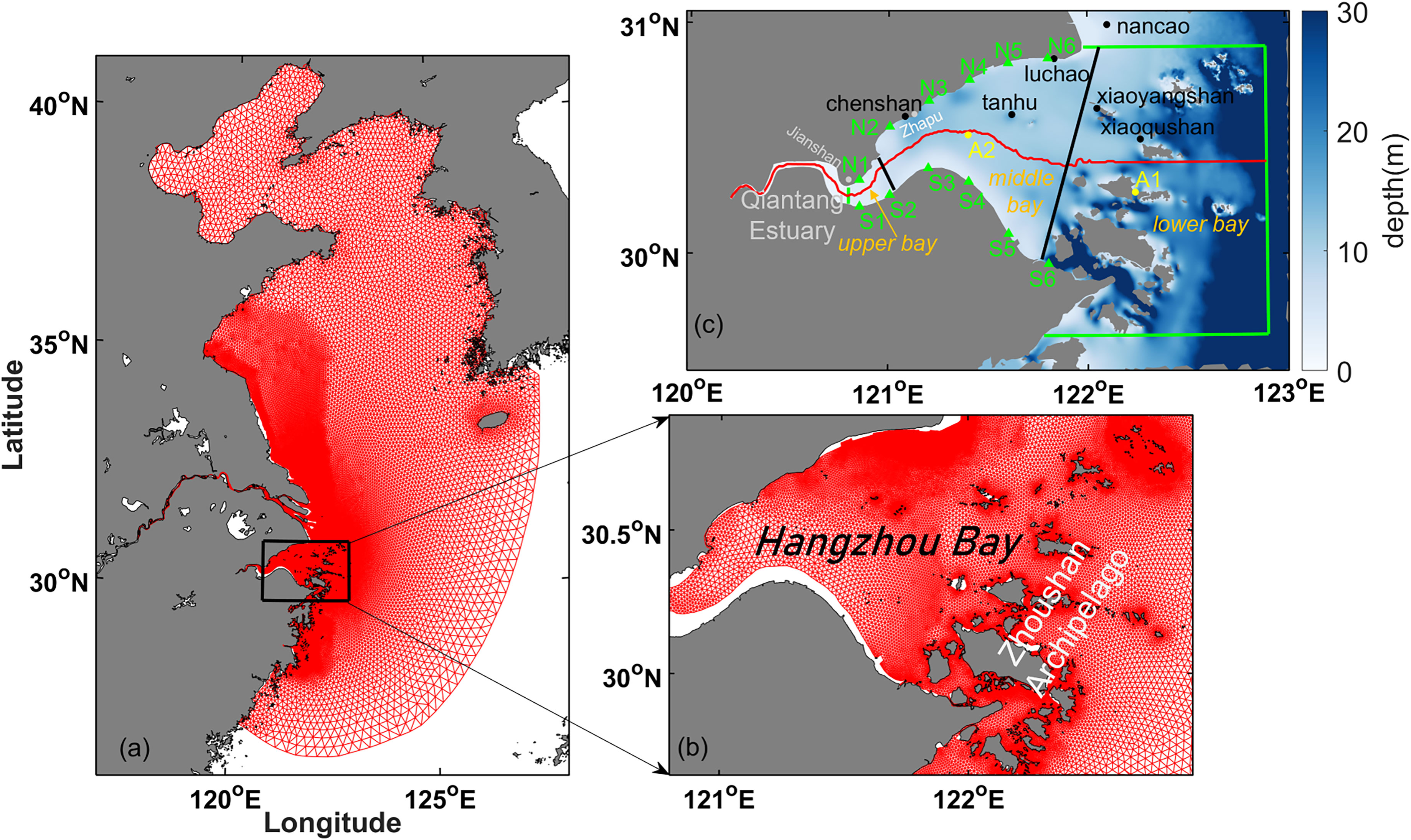
Figure 1 (A) Finite Volume Community Ocean Model (FVCOM) grids. (B) Zoomed-in view of FVCOM grids for Hangzhou Bay. (C) Bathymetry of Hangzhou Bay. The solid red line represents the center axis of Hangzhou Bay. The green lines and the coastline envelope the control volume for tidal energy budget analysis. The black lines divide Hangzhou Bay into three parts for analysis in Table 3. The black solid dots are used for water level validation. The green triangle marked virtual stations N1~N6 and S1~S6. The yellow solid dots marked A1 and A2 for momentum balance analysis.
2.2 Model validation for the control run
The hourly water levels from the present run were validated at 6 tidal gauge stations (Figure 2A). To provide a quantitative evaluation of the model performance, Taylor and Target diagrams were also plotted (Figures 2B, C). The Taylor diagram employs colorful symbols to represent 6 tidal stations. It conveys the correlation coefficient, centered RMSE (root mean square error), and the standard deviation ratio of simulated and observed results through the relative positioning of a point (simulated results) to a reference (Taylor, 2001). The target diagram presents pattern statistics and bias, enabling evaluation of their individual contributions to the total RMSE (Jolliff et al., 2009).

Figure 2 (A) Validation of predicted water level at six tidal gauges. (B) Taylor and (C) Target diagrams for water level validation.
The direct comparison between simulated results and tidal gauge data is shown in Figure 2A, and the overall trend is quite consistent. The error analysis of the tidal gauge stations is presented in Figures 2B, C. The normalized RMSEs of all tidal gauge stations are less than 0.5, and the correlation coefficients are all above 0.90. Therefore, the tidal verification results indicate that the hydrodynamic model is robust and suitable for further analysis.
2.3 SLR trends
IPCC AR6 provides a set of new emission scenarios driven by different socio-economic models, known as shared socio-economic pathways (SSPs). In this study, three pathways were selected, including SSP 245, SSP 370, and SSP 585. Moreover, a set of contributing factors were considered to provide a careful estimation of future SLR in Hangzhou Bay (Sung et al., 2021). Sea level changes caused by ocean thermal expansion was estimated with results from the CMIP6 (the sixth international coupled model comparison project) climate models (Supplementary Table 1). The contribution of the Greenland and Antarctic ice sheets, glaciers, and groundwater storage is from Fox-Kemper et al. (2021). Liang et al. (2022) estimated the rate of glacial isostatic adjustment (GIA) in Hangzhou Bay is 0.12 mm yr-1. Wang et al. (2012) estimated that the rate of land subsidence in the northern Hangzhou Bay can be up to 2 mm yr-1. Overall, the relative SLR rate in Hangzhou Bay can be acquired by considering the above factors, and the mean sea level of Hangzhou Bay is predicted to increase by 0.31 – 1.15 m by 2100 (Table 1).

Table 1 Individual contributions for relative SLR in Hangzhou Bay by 2100 (unit: m).
2.4 Numerical experiments
Two sets of runs were conducted to investigate the impact of SLR on tides in Hangzhou Bay. The first set of runs aims to predict future tidal ranges along the northern and southern shore of the bay under the 9 SLR scenarios summarized in Table 1. The second set was designed to explore whether tidal amplitudes in Hangzhou Bay linearly increased with SLR; and 6 runs with mean sea level changes of -1, -0.5, 0.5, 1, 1.5, and 2 m were conducted. In all experiments, mean sea level changes were added to the open boundary of the model. Particularly, the experiment with 1 m increase (hereafter: Future run), which is close to the predicted maximum local SLR in 2100 (Table 1), was selected for in-depth analysis in order to reveal the underlying physics of how tides response to SLR.
3 Results
In this section, the tidal characteristics under the current sea level will be first presented. Next, how the dominant tidal constituents along the center axis, the northern coastline and southern coastline of Hangzhou Bay change with SLR will be investigated. Then, an analysis of tidal energy budget and momentum balance will be conducted to help understand the underlying physics.
3.1 Tides of present sea level
The co-tidal charts for the four major constituents (M2, S2, K1, and O1) under current sea level are plotted in Figure 3. Among the four constituents, semi-diurnal tides dominate: the maximum amplitudes of M2 and S2 exceed 2.40 m and 0.75 m, respectively, while the diurnal tides are significantly weaker, with maximum amplitudes of 0.35 m and 0.21 m for K1 and O1, respectively. Although all tidal amplitudes increase from the lower bay to the upper bay, semi-diurnal tides (over 100% increase) have stronger amplification than diurnal tides (c.a. 20% increase).
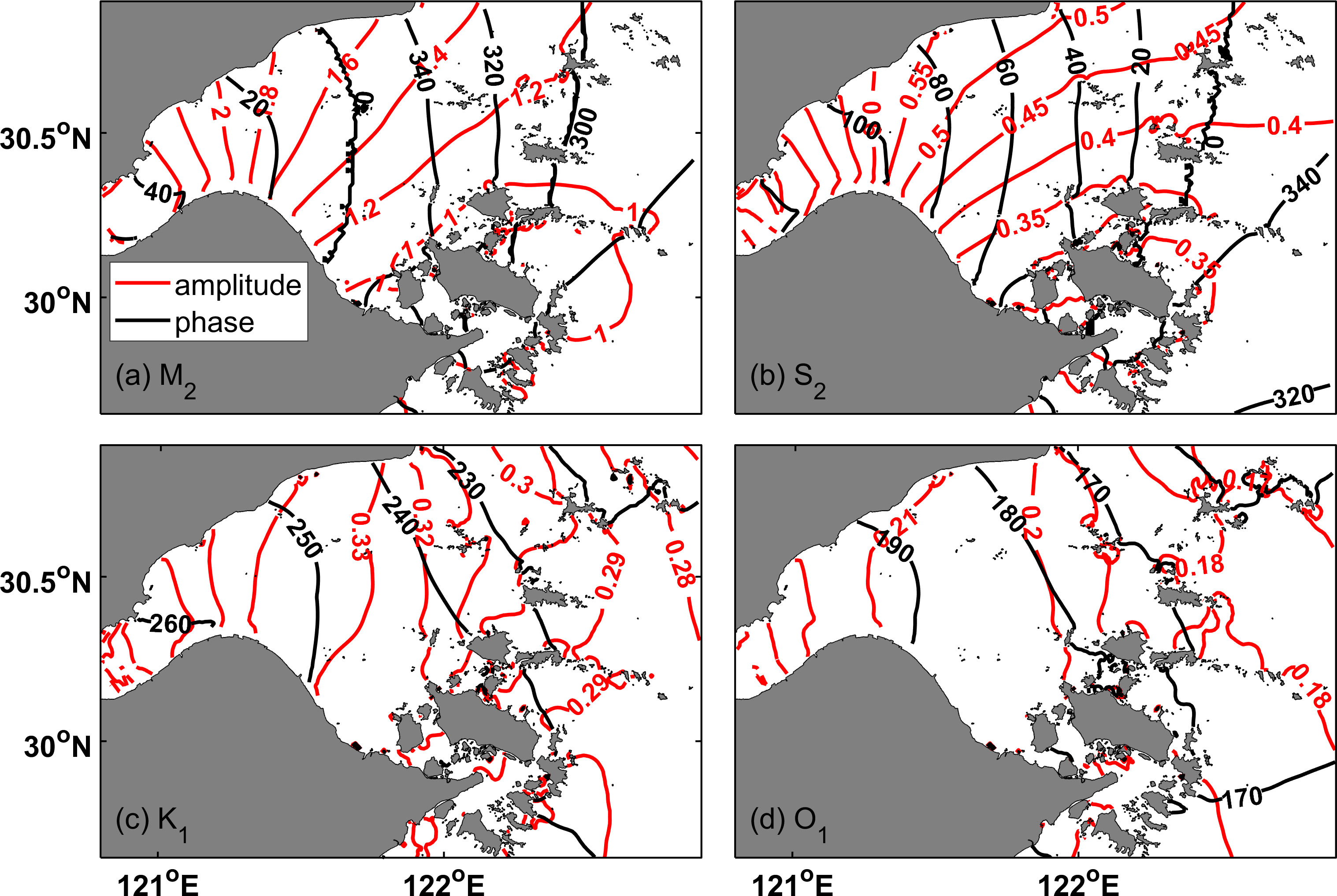
Figure 3 Co-tidal charts for (A) M2, (B) S2, (C) K1, and (D) O1. Red and black contours are for tidal amplitudes and phases, respectively.
The angles between co-amplitude and co-phase lines (Figure 3) and the phase differences (△Φ) between tidal velocity and tidal water level (Figure 4) are used here to indicate whether the tidal constituents are progressive waves (perpendicular lines and 0 phase difference) or standing waves (parallel lines and π/2 phase difference) (Lee et al., 2017). The semi-diurnal and diurnal tides show different behaviors. Both M2 and S2 are progressive waves near the bay mouth; in the mid-bay, they are progressive waves near the northern shore but standing waves in the southern shore; in the upper bay, they are mostly standing waves except within the central channel. Since progressive waves transport energy much more efficiently than standing waves (Lee et al., 2017), the semi-diurnal tidal energy mostly comes in along the northern shore of Hangzhou Bay. In contrast, diurnal tides are mostly standing waves throughout the bay, suggesting the diurnal tide carries much less energy into the bay compared to semi-diurnal tides. The tidal ellipses show that the M2 tidal currents are much stronger (1 m s-1) than those of the other tidal components (less than 0.3 m s-1), and the tidal currents in Hangzhou Bay are mostly rectilinear (Figure 4); therefore, the major axis of the tidal ellipses well represent the direction of tidal energy flux.
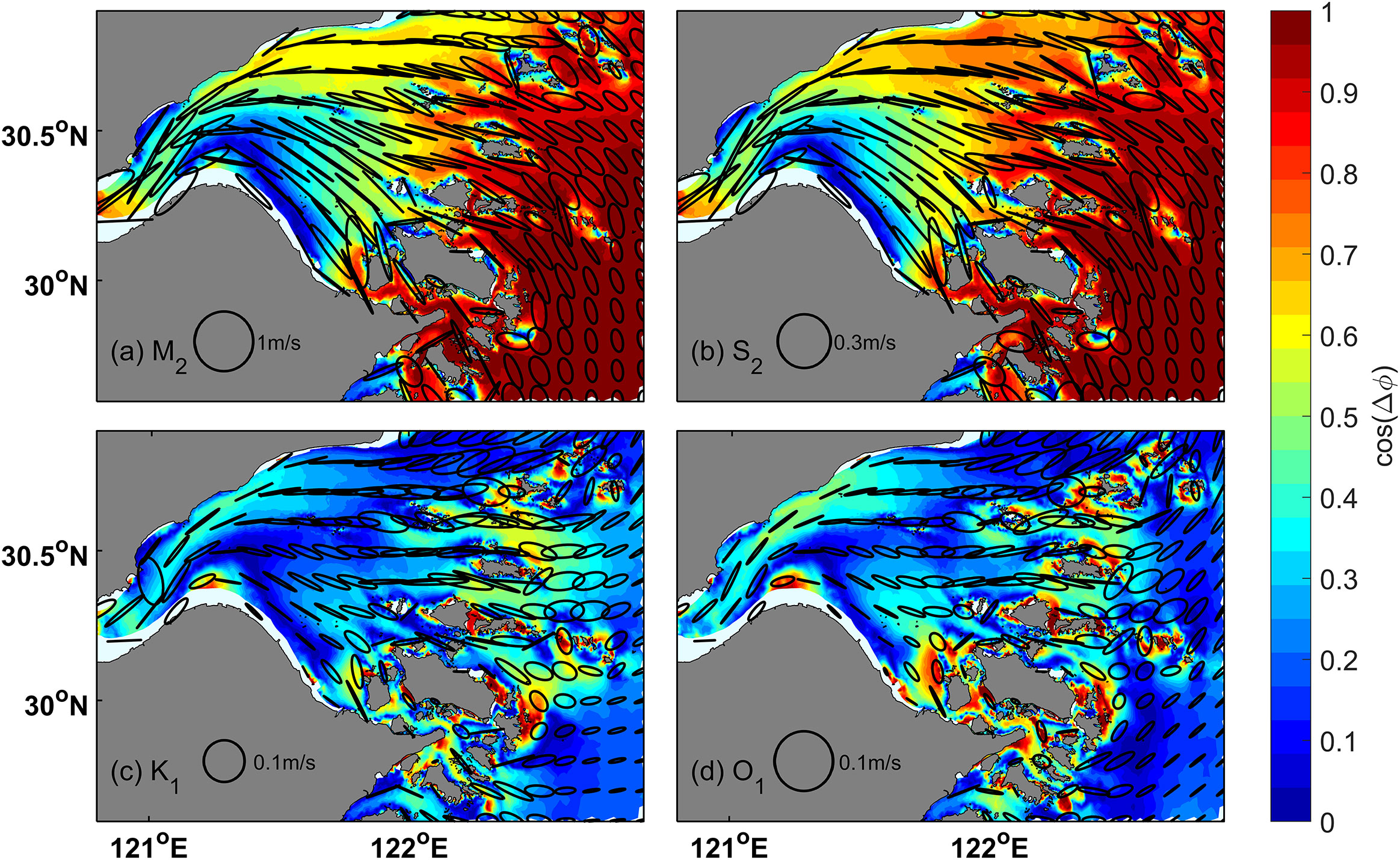
Figure 4 Tidal ellipses for (A) M2, (B) S2, (C) K1, and (D) O1. The shaded contours show the phase differences between tidal velocity and water level.
3.2 Prediction of future tides
Given M2 and K1 tide are much stronger than other semi-diurnal and diurnal tidal constituents, the following analysis focuses primarily on these two tidal components. To examine the impact of SLR on the M2 and K1 tidal amplitudes along the northern and southern shores of Hangzhou Bay, six points were selected on each shore, ranging from the upper bay to the lower bay (N1 – N6 and S1 – S6 in Figure 1C). As shown in Figure 5, the M2 tidal amplitude on the northern shore increases from the mouth of bay to the head in both present and SLR scenarios; whereas on the southern shore, the amplitude initially increases towards the upstream but then decreases slightly at the bay head under current sea level. At the same longitude, the amplitude of N1 is slightly smaller than S1, while the amplitudes of N2 and N3 are larger than S2 and S3. Additionally, the amplitudes of N4 to N6 are larger than S4 to S6. These observations indicate an asymmetry in the amplitudes between the north and south shores. In fact, the incoming tidal waves (northwestwards) are restricted by the funnel-shaped geometry of the bay, so that flood currents converge off the northern shore, resulting in stronger tides there (Xie et al., 2009). Moreover, the tidal wave in Hangzhou Bay can be regarded as a Kelvin wave, resulting in larger wave amplitude on the right side of wave propagation direction (Xie et al., 2017a). In contrast to M2, the present K1 amplitude initially increases from the bay mouth to the upper bay, but showed a 5-10% decrease at the bay head, with relatively small differences between the two shores. Overall, with SLR, the amplitudes of both M2 and K1 experience the greatest increase at the bay head and least increase at the bay mouth. The M2 amplitudes are up to 0.2 m and 0.25 m larger at N1 and S1, respectively, amounting to 10% increase. The amplitude increase is more significant for K1 at the bay head and approximately 25% increases are observed at N1 and S1.
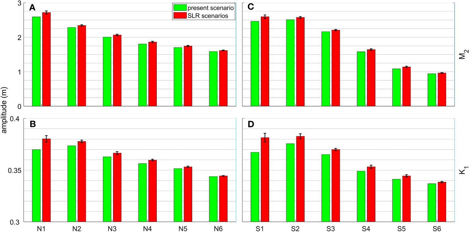
Figure 5 (A) M2 and (B) K1 tidal amplitude at N1 – N6 on the northern shore of Hangzhou Bay under present and future scenarios. (C, D) Same as (A, B), but for the southern shore. The red bars represent the predicted median values, and the error bars show the standard deviation of amplitudes from “min”, “median”, “max” projections of the three climate scenarios.
To provide a more comprehensive view, the spatial distribution of tidal amplitudes is presented in Figure 6. In both the Present and Future scenarios, the amplitude of the M2 tidal component gradually increases from the lower bay to upper bay, due to the convergence of coastlines. SLR leads to an increase in the M2 amplitude and a decrease in its phase, indicating a faster propagation of tidal waves in the bay. The changes in the amplitude and phase of the K1 tidal component are similar to those of M2 in terms of spatial pattern, but their magnitudes are smaller. In the Present run, the maximum flow velocity of M2 tide is observed in the upper bay, while the maximum flow velocity of K1 tide is at the mouth of the bay. However, with SLR, the flow velocity of M2 tides decreases in the upper bay and mid-bay, while increasing in the archipelago region, and the flow velocity of K1 tides decreases throughout the bay.
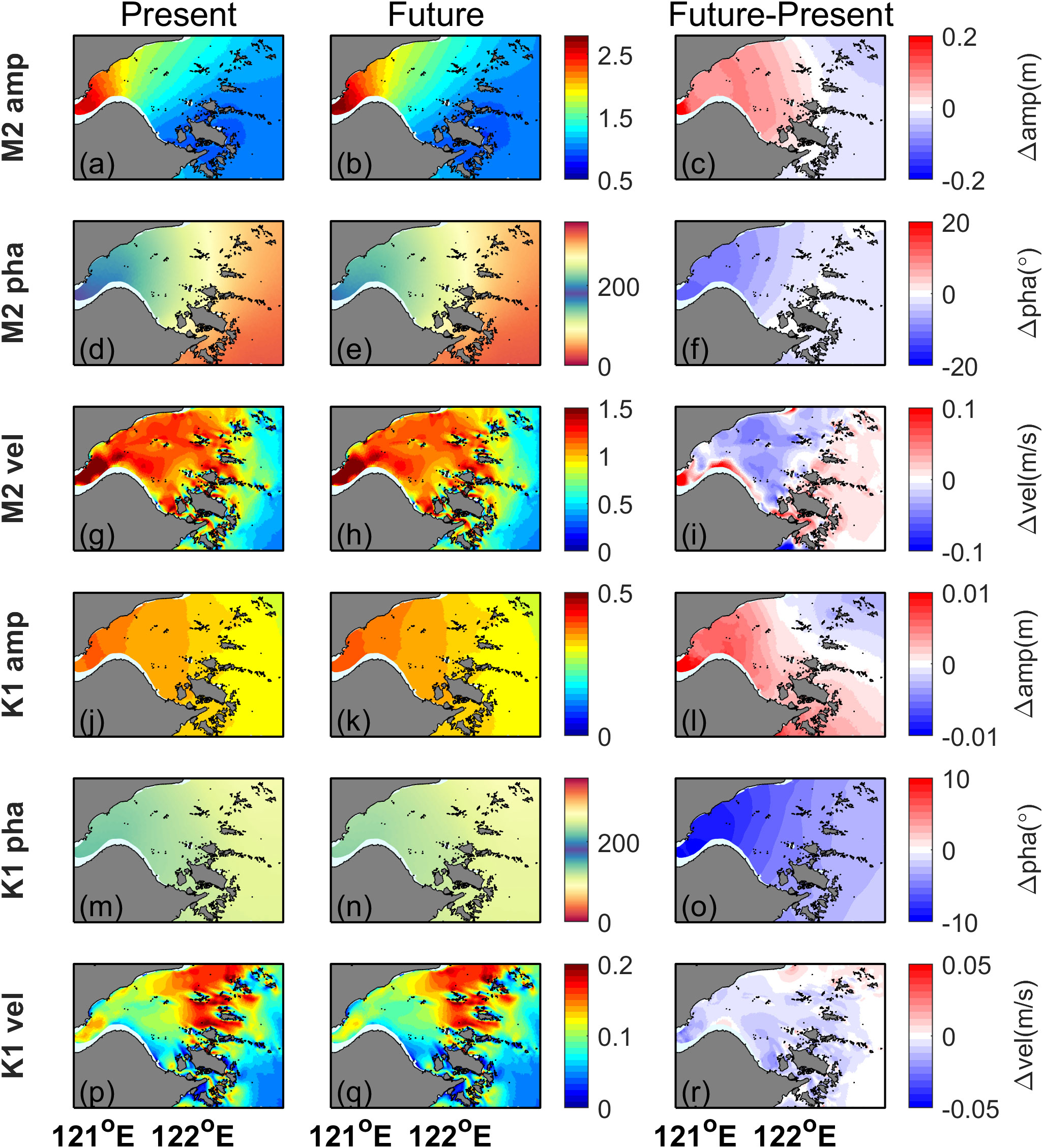
Figure 6 Spatial distribution of M2 tidal amplitude from (A) Present run and (B) Future run. (C) Tidal amplitude differences between Future run and Present run. (D-F) Same as (A-C), but for water level phases. (G-I) Same as (A-C), but for the major axis of tidal ellipse. (J-R), same as (A-I), but for K1 tide.
Next, whether tidal amplitudes increase linearly with SLR in Hangzhou Bay is investigated. Figures 7A, B show the tidal amplitudes of M2 and K1 along the central axis of Hangzhou Bay with different mean sea level. West of the archipelago (c.a. 122.2°E), the amplitudes of M2 and K1 grow with rising sea level. However, the opposite trend is observed in the archipelago region. In Figures 7C, D, ΔA/Δh was used to indicate the sensitivity of amplitude changes to SLR, where ΔA and Δh respectively represents the changes in tidal amplitude and mean sea level. In the mid-bay and upper bay, the growth rate of tidal amplitude reduces with increasing SLR. Conversely, in the archipelago region, the reduction rate of tidal amplitude grows with rising sea level. The variation of ΔA/Δh for K1 is generally similar to that of M2. However, the K1 amplitudes in the mid-bay and upper bay almost cease to increase when the SLR becomes higher than 1.5 m. This is closely linked to the resonance behavior of K1 tidal wave when its wavelength grows well beyond four times of the bay length, given the speed of shallow water wave increases with SLR (Zhong et al., 2008; Pickering et al., 2017). Overall, these results suggest that the response of tidal amplitudes to SLR is nonlinear in Hangzhou Bay and the tidal amplitudes are close to maximum when the SLR is over 1.5 m.
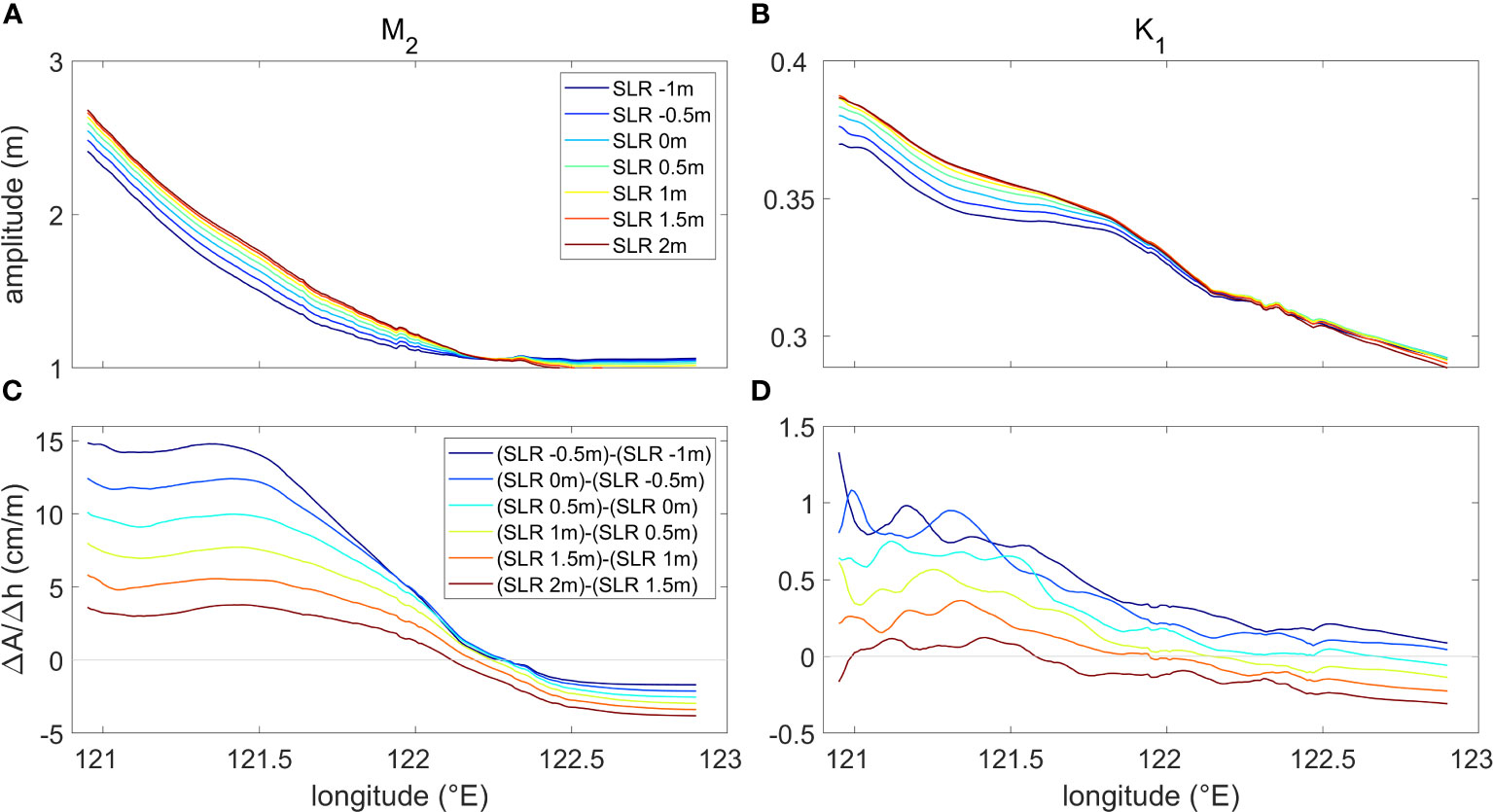
Figure 7 (A) Tidal amplitude of M2 along the center axis of Hangzhou Bay with different mean sea level. (B) Same as (A), but for K1. (C, D) Same as (A, B), but for the ratio of tidal amplitude change (ΔA) to sea level change (Δh).
3.3 Energy budget analysis
To understand the physical mechanism of SLR effects on tides, energy budget of the M2 and K1 tides is analyzed. To simplify the analysis, nonlinear interactions between different tidal constituents are ignored and additional Present and Future runs with only M2 or K1 tide are conducted. Results from these one-tidal-component runs are used for the following analysis.
By integrating the energy equation over the control volume, which is bounded by the northern and southern shore of Hangzhou Bay, the Qiantang River mouth in the upper bay, and a hypothetic boundary at the bay mouth (see the green lines in Figure 1C for upper bay and lower bay boundaries), and averaging over a tidal cycle, the following equation was obtained:
where< > denotes time averaging over the tidal cycle, u and v represent the velocity components in the x (eastward) and y (northward) directions, respectively, is the density of water, p represents barotropic pressure related to tidal water level, is the normal vector of the control volume surface, =(u, v) is the horizontal velocity, and KH and KV are the horizontal and vertical eddy viscosity, respectively. The left-hand side of Equation 1 describes the tidal energy flux () which includes the pressure work term and advection term, while the right-hand side consists of dissipation terms related to vertical and horizontal shear flow. Given the advection of tidal kinetic energy is generally neglectable, the left-hand side can be rewritten as:
where g is the gravity acceleration, H is the water depth along the lateral boundary of the control volume and η is the tidal water level. Since the surface stress is zero, the first term on the right-hand side in Equation 1 represents the energy dissipation due to bottom friction and can be further simplified as:
where CD is the bottom drag coefficient, is the bottom friction, and is the bottom velocity. The other two terms on the right-hand side in Equation 1 describe the dissipation within the water column and are hereafter regarded as vertical and horizontal dissipation, respectively.
The energetics of M2 and K1 integrated over the control volume are summarized in Table 2. It is worth noting that the energy flux term (Equation 2) is further divided into two parts: the incoming energy flux which represents the energy comes in from the offshore boundary and the outgoing energy flux which represents the energy goes westward into the Qiantang Estuary. At the present sea level, approximately 65% of the M2 tidal energy entering the control volume is dissipated due to friction in the bottom boundary layer (Equation 3), while approximately 24% is dissipated due to horizontal shear. The remaining dissipation is due mostly to vertical shear in the upper water column. It is worth noting that the horizontal dissipation is explicitly calculated in this work, in contrast to the inferred values in previous studies (e.g., Ren et al., 2021). The residual (the difference between the total dissipation and the net energy flux) due to numerical errors is within 5%, which is comparable to other studies (e.g., Lee et al., 2017). In contrast, the tidal energetics of K1 is two orders of magnitude smaller than that of M2. Nevertheless, similar to M2, the bottom friction dissipates nearly 60% of the tidal energy, the horizontal dissipation accounts for 23%, and the rest dissipation is attributed to vertical shear in the water column.
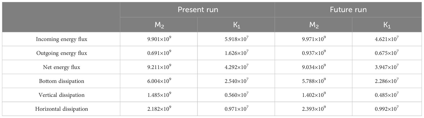
Table 2 Volume-integrated energetics of M2 and K1 tide over Hangzhou Bay from Present run and Future run (unit: W).
In the Future run, the incoming energy flux of M2 surprisingly only increases by 1% due to the reduction of tidal amplitude in the offshore. This increase is disproportional to the increase of cross-sectional area at the offshore boundary. The outgoing energy flux significantly increased by 36%, which is consistent with the increase in tidal amplitude at the bay head. The decrease in bottom dissipation is attributed to the reduction of tidal velocity across most regions of Hangzhou Bay (Figure 6I). Similarly, vertical dissipation also decreases. Notably, horizontal dissipation exhibits the largest change, with an increase of approximately 10%. Therefore, horizontal dissipation is the primary factor contributing to the energy changes in Hangzhou Bay. In contrast to M2, the incoming and outgoing energy flux of K1 experience a significant decrease. This reduction in outgoing energy flux suggests that the energy flux of standing waves is highly sensitive to phase changes. Similar to M2, the bottom and vertical dissipation of K1 decrease, while the horizontal dissipation increases.
Figures 8A, B indicate that there is significant dissipation of M2 tidal energy in the upper and mid-bay. Figure 8C demonstrates that SLR leads to enhanced bottom dissipation in the archipelago region, indicating an increase in bottom velocity in this area. This increase is attributed to the higher tidal current velocity in the future run (Figure 6I). Conversely, the tidal current velocity in the mid-bay is decreasing, resulting in reduced bottom dissipation. The vertical dissipation is consistent with the bottom dissipation. Strong horizontal shear occurs in narrow channels around the islands, leading to high horizontal dissipation in the archipelago area (Figures 8G, H). With SLR, horizontal dissipation around the islands increases significantly (Figure 8I). The general spatial pattern of tidal dissipation for K1 is similar to that of M2 (c.f. Figures 8, 9). However, unlike M2, the dissipation in the archipelago area shows both decreases and increases for K1 (Figures 9C, F, I).
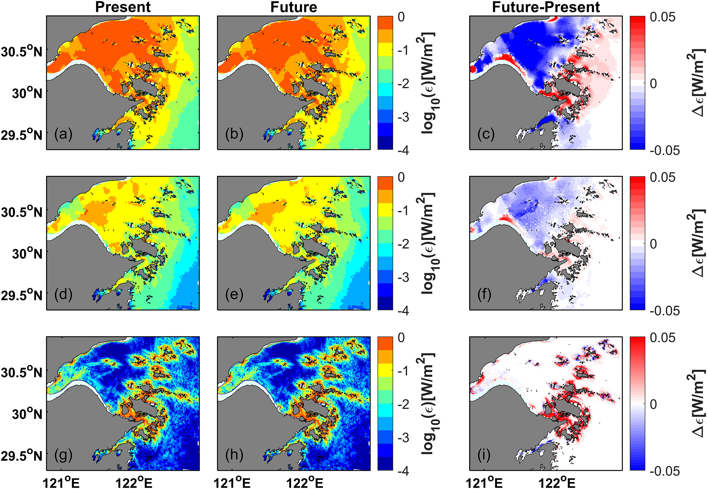
Figure 8 Bottom dissipation rate of M2 tide from (A) Present run and (B) Future run. (C) Differences of bottom dissipation rate between Future run and Present run. (D-F) Same as (A-C), but for vertical dissipation. (G-I) Same as (A-C), but for horizontal dissipation.
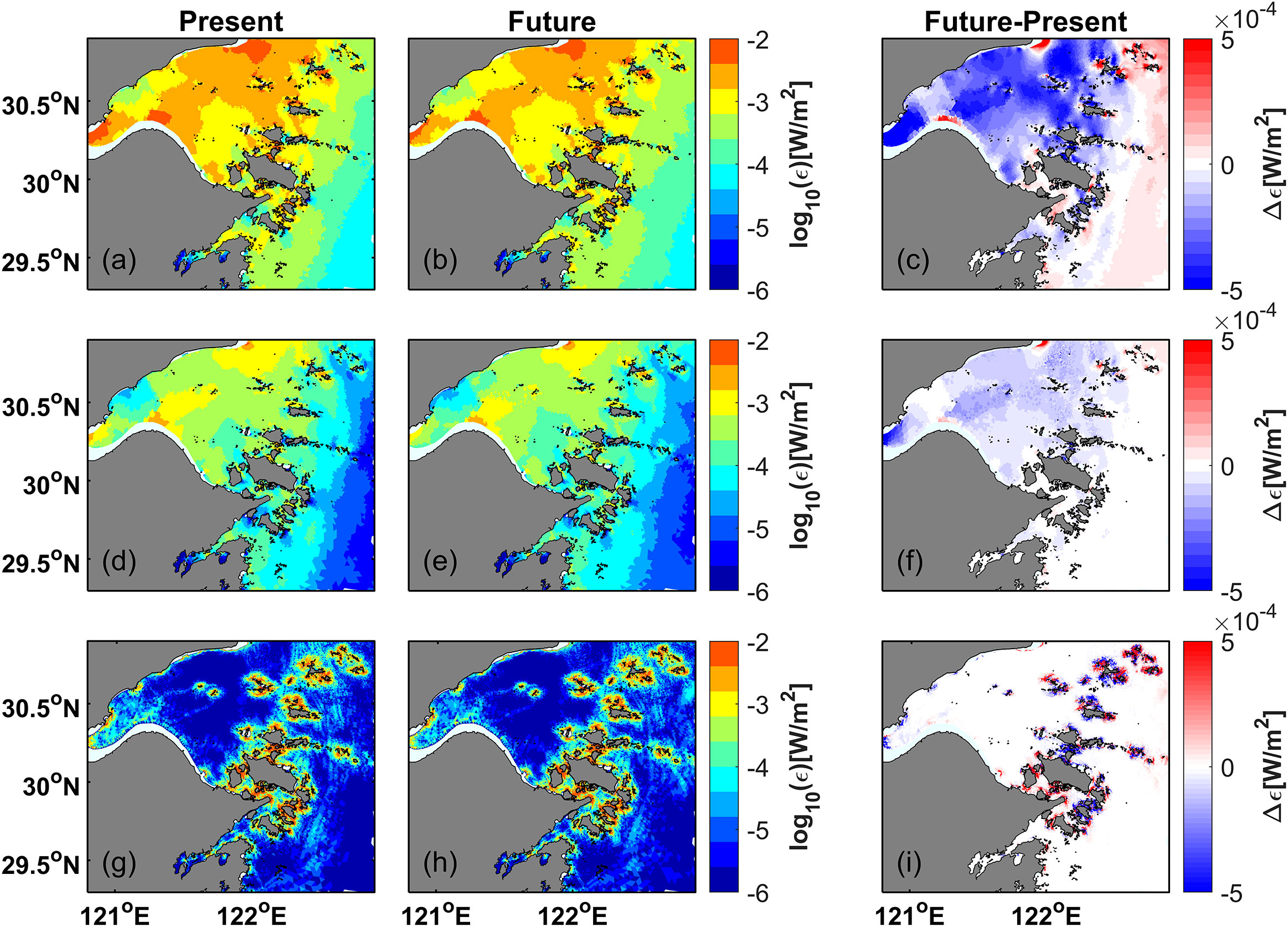
Figure 9 Bottom dissipation rate of K1 tide from (A) Present run and (B) Future run. (C) Differences of bottom dissipation rate between Future run and Present run. (D–F) Same as (A–C), but for vertical dissipation. (G–I) Same as (A–C), but for horizontal dissipation.
Horizontal dissipation is often neglected in other bays or coastal ocean [e.g., Yellow sea shelf (Feng et al., 2019); Chesapeake Bay and Delaware Bay (Lee et al., 2017)] due to its relatively small contribution. However, this term accounts for nearly a quarter of the tidal energy budget in Hangzhou Bay, which requires further investigation. Strong horizontal shear can take place in the archipelago area due to several reasons (Figures 10A, C). The narrow channels among the islands can amplify tidal currents, resulting in horizontal shear with ambient currents. In addition, similar to differential advection in estuaries, the lateral variations in horizontal velocity associated with boundary friction can also generate strong horizontal shear. With SLR, the horizontal shear of the M2 constituent around the islands intensifies (Figure 10B), which is closely linked to the enhanced tidal current in this region (Figure 6I). In contrast, the horizontal shear of the K1 constituent around the islands shows less increase (Figure 10D).
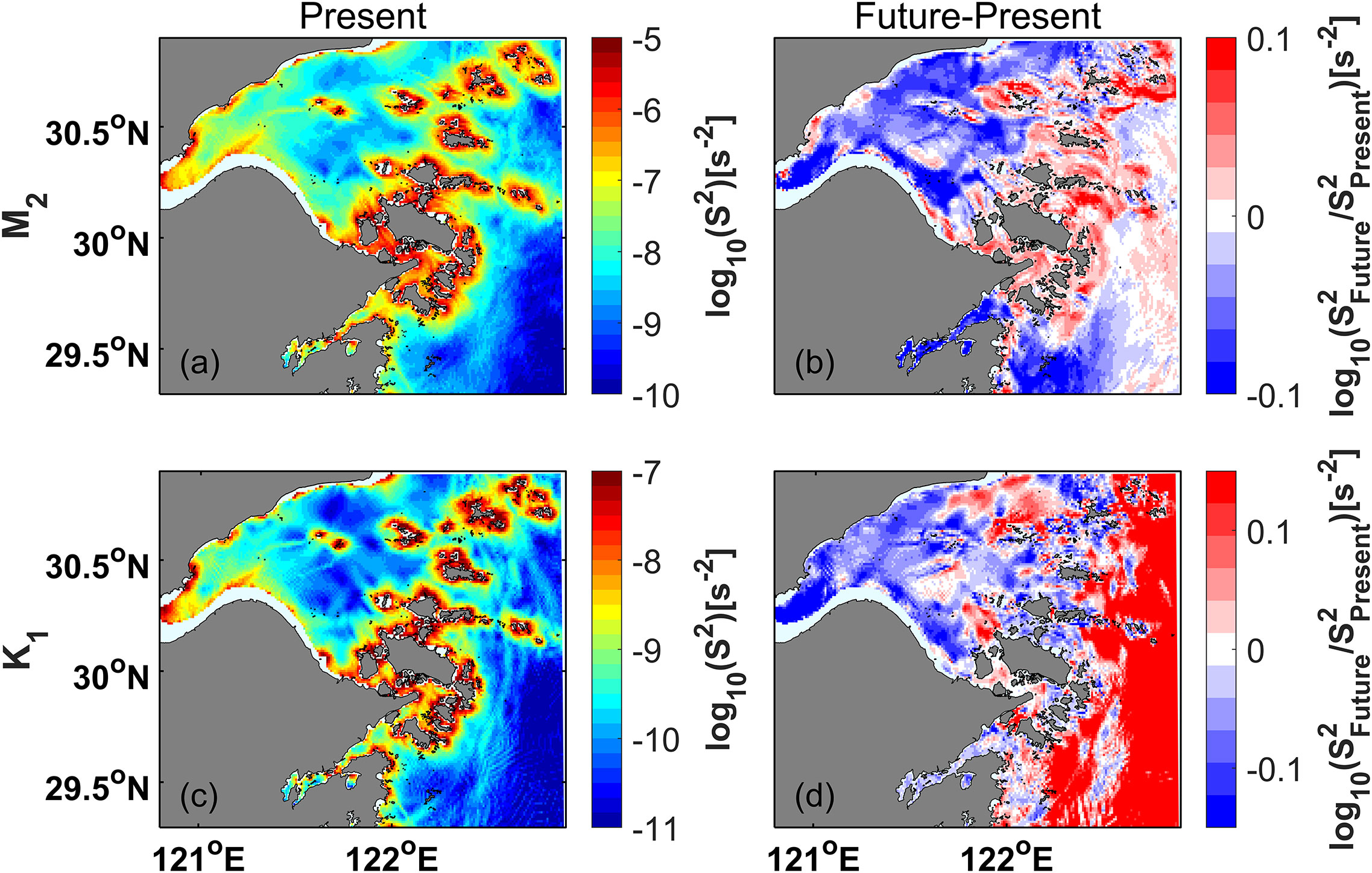
Figure 10 (A) Depth-averaged horizontal shear of M2 tidal flow from Present run. (B) Differences of the M2 horizontal shear between Future run and Present run. (C, D) Same as (A, B), but for K1 tide.
The above results suggest that most horizontal dissipation takes place in the archipelago region. To further quantify, Hangzhou Bay is divided into three parts: the upper bay, the mid-bay, and the archipelago area (see black lines in Figure 1C). Table 3 shows that although the horizontal dissipation of the M2 constituent increases in all three regions after SLR, the increase in the archipelago area is two orders of magnitude greater than that in the other two regions. The horizontal dissipation of the K1 constituent decreases in the upper bay and mid-bay after SLR, while it increases in the archipelago area. Therefore, indeed the presence of the archipelago leads to the much higher horizontal dissipation in Hangzhou Bay and plays an important role in changing tides.

Table 3 Volume-integrated horizontal dissipation of M2 and K1 tide over the three parts of Hangzhou Bay (see Figure 1) from Present run and Future run (unit: W).
3.4 Momentum balance analysis
To gain a better comprehension of the tidal dynamics, momentum balance was examined at two stations (A1 and A2, Figure 1C) with the following momentum equation:
where is the Coriolis parameter. The five terms in Equation 4 describe the local acceleration, advection, Coriolis force, pressure gradient force, and bottom friction, respectively.
Station A1 is located in a narrow channel, which is selected to investigate the tidal dynamics around islands. Station A2 is located at the central channel of the mid-bay which is used to study the typical tidal dynamics of the main bay. Figure 11 shows the time series of each term over one tidal cycle. At Station A1, M2 tide behaves as progressive waves, given the momentum balance is primarily between advection and barotropic pressure gradient (Figure 11A). With SLR, both the advective term and barotropic pressure gradient term experience slight increments, but the momentum balance remains between these two terms (Figure 11B). Furthermore, there are no significant changes in the magnitude and phase of tidal velocity and water level (Figure 11C), indicating that SLR does not alter the progressive wave characteristics of the M2 tide in the archipelago area. At Station A2, the momentum balance of M2 tide is mainly between local acceleration and barotropic pressure gradient, suggesting standing waves (Figure 11D). It is worth noting that, friction also plays an important role at A2, given the strong tidal current and shallow bathymetry there. SLR leads to a slight reduction in the barotropic pressure gradient term, a minor increase in the local acceleration term, and a marginal decrease in the phase of both water level and flow velocity (Figures 11E, F). However, the phase differences between them do not show significant changes.
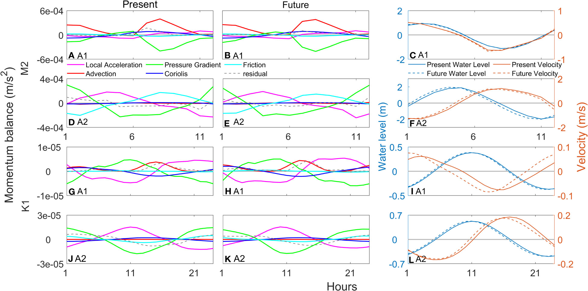
Figure 11 (A) Time series of local acceleration (magenta line), advection (red line), pressure gradient force (green line), Coriolis force (blue line), bottom friction (cyan line), and residual (dashed gray line) at A1 from M2 only run under current sea level. (B) Same as (A), but with 1 m sea level rise. (C) Time series of water level (blue lines) and velocity (orange lines) of M2 tide at A1. (D-F) Same as (A-C), but for M2 tide at A2. (G-L), same as (A-F), but for K1 tide.
K1 tide at both A1 and A2 exhibit standing wave characteristics. The momentum balance is primarily between the pressure gradient term and the local acceleration term (Figures 11G, H, J, K). At Station A1, both terms increase after SLR (c.f. Figures 11G, H). In addition, the phase differences between tidal velocity and water level deviates from π/2, suggesting decreased resonance of K1 tide in the archipelago area (Figure 11I). At Station A2, SLR nearly preserves the magnitudes of all terms in the momentum equation (c.f. Figures 11J, K), and marginal changes are observed in tidal velocity and water level (Figure 11L).
4 Discussion
4.1 Changes in tidal range
Previous studies have shown that the response of tides to SLR can be spatially heterogeneous and nonlinear (Pickering et al., 2012; Pelling et al., 2013; Lee et al., 2017; Ross et al., 2017). For instance, Lee et al. (2017) found that the tidal range increases in Delaware Bay with SLR, ranging from 2 cm at the mouth of estuary to 25 cm in the upper bay. Similarly, this study also found that the tidal amplitude change in Hangzhou Bay is spatially nonuniform, which generally amplifies towards the upper bay. This contrasts with the alternating increase and decrease of tidal amplitudes on the open shelf due to shift of amphidromic points (Carless et al., 2016; Idier et al., 2017). Therefore, between estuaries and open shelves, there can be significant differences in tidal response to SLR.
On the other hand, this study showed that the growth of tidal amplitude reduces with increasing SLR in the mid-bay and upper bay. The tidal amplitudes become less sensitive to sea level changes in Hangzhou Bay once SLR exceeds 1.5 m. In their modeling study of Chesapeake and Delaware bays, Lee et al. (2017) also showed that the mean tidal range difference is nearly the same under SLR 0.75 m and SLR 1 m scenarios, which implies that when future SLR exceeds 0.75 m, the sensitivity of tidal range amplitudes in both bays to sea level changes diminishes. In contrast, in a companion study of Lee et al. (2017); Ross et al. (2017) examined the response of tidal amplitude to past SLR based on long term historical records at multiple tidal gauge stations. They found the response of M2 amplitude to past SLR in both bays were approximately linear. The discrepancy is likely related to the resonance behavior of tidal waves. The tidal amplitude is most sensitive to sea level changes when the tidal wave length is close to 4 times of the bay length and strong resonance occurs (Zhong et al., 2008). As the wave length grows beyond this sweet spot with increasing sea level, the tidal amplitude becomes less sensitive to sea level changes.
Moreover, the maximum tidal range is critical in face of tidal nuisance flooding. Therefore, the tidal ranges at the northern (N1-N6) and southern shore (S1-S6) stations were examined. Maximum tidal ranges during spring and neap tide from future scenario (1m SLR) were compared to those from the present scenario simulation (Figure 12). It is clear that the impact of SLR on tidal range is greater during spring tides than during neap tides. In particular, the increase of tidal ranges at upper bay stations (N1 and S1) was over 1 m during spring tide but less than 0.3 m during neap tide. Similarly, Pickering (2014) also showed that the tidal range change with SLR is greater during spring tide than during neap tide on the European Shelf.
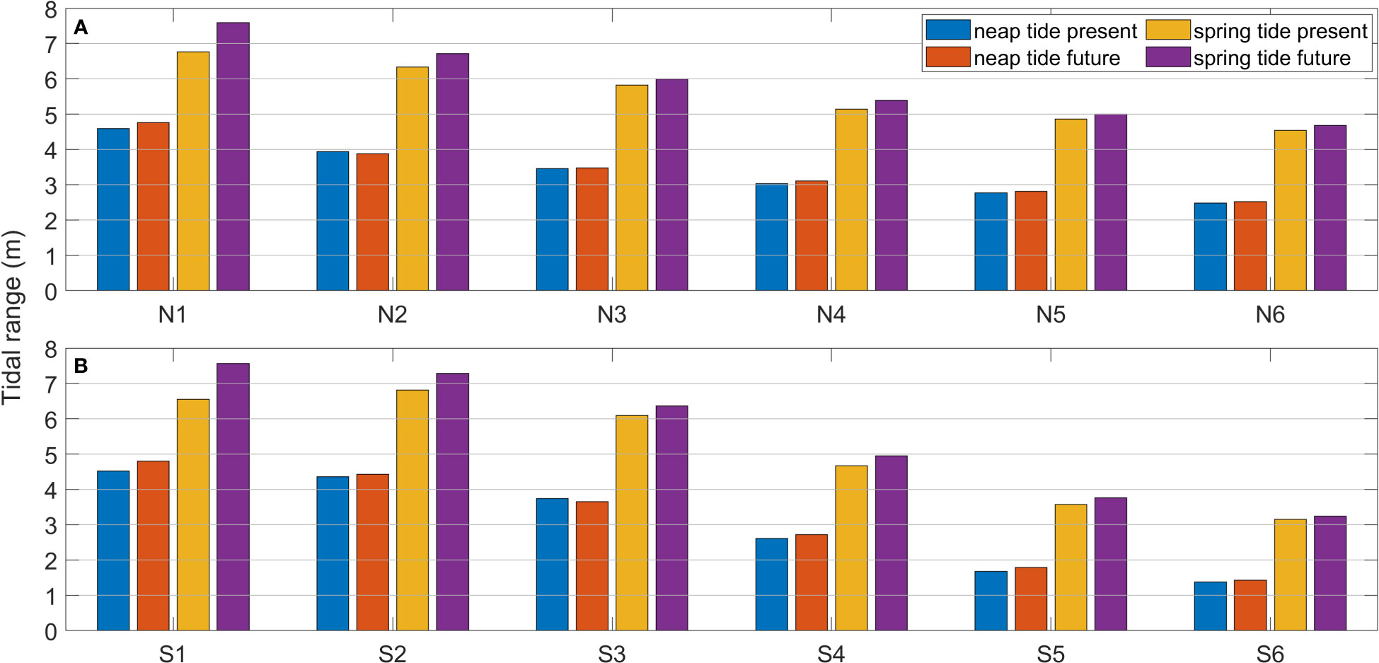
Figure 12 The maximum tidal range during neap and spring tides at (A) N1 – N6 on the northern shore and (B) S1 – S6 on the southern shore of Hangzhou Bay under present and future scenarios.
4.2 Changes in tidal energy
Previous studies on tidal energy dissipation in Hangzhou Bay have primarily focused on bottom friction (Wu et al., 2018; Liang et al., 2022). Liang et al. (2022) found that bottom dissipation increases around the Zhoushan Archipelago and the Andong tidal flat, while decreasing in other areas of Hangzhou Bay with SLR, consistent with this study. On the other hand, previous studies assumed that horizontal dissipation is negligible; nevertheless, this study has revealed that horizontal dissipation in the archipelago region is significant, constituting 23% of the total dissipation. Following SLR, the proportion of horizontal dissipation increases, suggesting it plays a more important role in tidal energy budget in the future.
4.3 Impact of shoreline and morphological changes on tides
Studies of other estuaries or bays have shown that changes in shoreline can significantly affect coastal tides. For example, Feng et al. (2019) investigated the effect of coastline configuration on Yellow Sea tides by considering two scenarios with hard or soft shorelines. Their results showed that soft shorelines can allow more inundation of low-lying areas, thus dissipating more tidal energy and reducing tidal range. Additionally, Pelling et al. (2013) and Gao et al. (2014) have also demonstrated that coastal development can affect tidal dynamics in nearby areas. In fact, Hangzhou Bay has experienced extensive land reclamation in the past half century. The persistent influx of substantial sediment from the neighboring Changjiang River can also result in significant alterations to the coastline in this particular area (Chen et al., 1990; Xie et al., 2017b). Indeed, recent studies have shown that the changing bathymetry along with seasonal variations of river discharge can play an important role in tidal dynamics in the Qiantang Estuary (west of the Hangzhou bay proper, Figure 1C) (Xie et al., 2022). However, for simplicity, this study did not consider the impact of morphological evolution on tides. In addition, sensitivity experiments with river discharge turned on or off showed minimal impacts of river runoff on tides east of 121°E (not shown). Nevertheless, it is imperative for future research to delve deeper into the impact of morphological evolution and coastline modifications on the tides of Hangzhou Bay in a SLR era.
5 Conclusion
This study has investigated how tides in Hangzhou Bay respond to SLR with numerical simulations. The tidal amplitudes of both M2 and K1 were found to progressively increase from the lower bay to the upper bay with SLR. From the perspective of tidal energy budget, the incoming energy flux of M2 increased with SLR, but the horizontal dissipation in the Zhoushan Archipelago region increased as well, resulting in the relatively unchanged M2 amplitude near the bay mouth. In the mid-bay, the bottom and vertical dissipation of M2 decreased with SLR, leading to increased tidal amplitude. On the other hand, although SLR reduced the incoming energy flux of K1, the decreased bottom and vertical dissipation resulted in increased K1 amplitude in most parts of Hangzhou Bay.
Data availability statement
The raw data supporting the conclusions of this article will be made available by the authors, without undue reservation.
Author contributions
CL: Writing – original draft. FZ: Writing – review & editing, Conceptualization, Formal Analysis, Funding acquisition, Investigation, Project administration, Supervision. JJ: Writing – review & editing, Data curation, Investigation. YW: Writing – review & editing, Data curation, Investigation.
Funding
The author(s) declare financial support was received for the research, authorship, and/or publication of this article. This work was sponsored by the National Natural Science Foundation of China (42006151), the Innovation Program of Shanghai Municipal Education Commission (2021-01-07-00-08-E00102), and the Science and Technology Committee of Shanghai Municipal (No. 23ZR1420300).
Conflict of interest
The authors declare that the research was conducted in the absence of any commercial or financial relationships that could be construed as a potential conflict of interest.
Publisher’s note
All claims expressed in this article are solely those of the authors and do not necessarily represent those of their affiliated organizations, or those of the publisher, the editors and the reviewers. Any product that may be evaluated in this article, or claim that may be made by its manufacturer, is not guaranteed or endorsed by the publisher.
Supplementary material
The Supplementary Material for this article can be found online at: https://www.frontiersin.org/articles/10.3389/fmars.2023.1302800/full#supplementary-material
References
Carless S. J., Green J. M., Pelling H. E., Wilmes S. B. (2016). Effects of future sea-level rise on tidal processes on the Patagonian Shelf. J. Mar. Syst. 163, 113–124. doi: 10.1016/j.jmarsys.2016.07.007
Chen C., Beardsley R. C., Cowles G., Qi J., Lai Z., Gao G., et al. (2006). An unstructured grid, finite-volume coastal ocean model: FVCOM user manual. SMAST/UMASSD 6, 78. doi: 10.5670/oceanog.2006.92
Chen J., Liu C., Zhang C., Walker H. J. (1990). Geomorphological development and sedimentation in Qiantang estuary and Hangzhou bay. J. Coast. Res. 6 (3), 559–572.
Edwards R. J. (2006). Mid-to late-Holocene relative sea-level change in southwest Britain and the influence of sediment compaction. Holocene 16 (4), 575–587. doi: 10.1191/0959683606hl941rp
Egbert G. D., Erofeeva S. Y. (2002). Efficient inverse modeling of barotropic ocean tides. J. Atmos. Oceanic Technol. 19 (2), 183–204. doi: 10.1175/1520-0426(2002)019<0183:EIMOBO>2.0.CO;2
Ezer T. (2013). Sea level rise, spatially uneven and temporally unsteady: Why the US East Coast, the global tide gauge record, and the global altimeter data show different trends. Geophys. Res. Lett. 40 (20), 5439–5444. doi: 10.1002/2013GL057952
Ezer T., Atkinson L. P., Corlett W. B., Blanco J. L. (2013). Gulf Stream's induced sea level rise and variability along the US mid-Atlantic coast. J. Geophys. Res.: Oceans 118 (2), 685–697. doi: 10.1002/jgrc.20091
Feng X., Feng H., Li H., Zhang F., Feng W., Zhang W., et al. (2019). Tidal responses to future sea level trends on the Yellow Sea shelf. J. Geophys. Res.: Oceans 124 (11), 7285–7306. doi: 10.1029/2019JC015150
Feng J. L., Li W. S., Wang H., Zhang J. L., Dong J. X. (2018). Evaluation of sea level rise and associated responses in Hangzhou Bay from 1978 to 2017. Adv. Climate Change Res. 9 (4), 227–233. doi: 10.1016/j.accre.2019.01.002
Fox-Kemper B., Hewitt H. T., Xiao C., Aðalgeirsdóttir G., Drijfhout S. S., Edwards T. L., et al. (2021). “Ocean, cryosphere and sea level change,” in Climate Change 2021: The Physical Science Basis. Contribution of Working Group I to the Sixth Assessment Report of the Intergovernmental Panel on Climate Change. Eds. Masson-Delmotte V., Zhai P., Pirani A., Connors S. L., Péan C., Berger S., Caud N., Chen Y., Goldfarb L., Gomis M. I., Huang M., Leitzell K., Lonnoy E., Matthews J. B. R., Maycock T. K., Waterfield T., Yelekçi O., Yu R., Zhou B. (Cambridge, United Kingdom and New York, NY, USA: Cambridge University Press), 1211–1362. doi: 10.1017/9781009157896.011
Gao G. D., Wang X. H., Bao X. W. (2014). Land reclamation and its impact on tidal dynamics in Jiaozhou Bay, Qingdao, China. Estuar. Coast. Shelf Sci. 151 (5), 285–294. doi: 10.1016/j.ecss.2014.07.017
Haigh I. D., Pickering M. D., Green J. M., Arbic B. K., Arns A., Dangendorf S., et al. (2020). The tides they are a-Changin': A comprehensive review of past and future nonastronomical changes in tides, their driving mechanisms, and future implications. Rev. Geophys. 58 (1), e2018RG000636. doi: 10.1029/2018RG000636
Hay C. C., Morrow E., Kopp R. E., Mitrovica J. X. (2015). Probabilistic reanalysis of twentieth-century sea-level rise. Nature 517 (7535), 481–484. doi: 10.1038/nature14093
Holleman R. C., Stacey M. T. (2014). Coupling of sea level rise, tidal amplification, and inundation. J. Phys. Oceanogr. 44 (5), 1439–1455. doi: 10.1175/JPO-D-13-0214.1
Horsburgh K. J., Wilson C. (2007). Tide-surge interaction and its role in the distribution of surge residuals in the North Sea. J. Geophys. Res.: Oceans 112 (C08003). doi: 10.1029/2006JC004033
Horton B. P., Shennan I. (2009). Compaction of Holocene strata and the implications for relative sea level change on the east coast of England. Geology 37 (12), 1083–1086. doi: 10.1130/G30042A.1
Hou F., Bao X., Li B., Liu Q. (2015). The assessment of extactable tidal energy and the effect of tidal energy turbine deployment on the hydrodynamics in Zhoushan. Acta Oceanol. Sin. 34, 86–91. doi: 10.1007/s13131-015-0671-2
Idier D., Paris F., Le Cozannet G., Boulahya F., Dumas F. (2017). Sea-level rise impacts on the tides of the European Shelf. Cont. Shelf Res. 137, 56–71. doi: 10.1016/j.csr.2017.01.007
Ji Y. J., Liu D. J., Huang P. Y., Huang C. L. (2015). Influence analysis of sediment dynamics and seabed evolution in adjacent channel under Zhoushan islands reclamation project. J. Waterway Harbor 36 (2), 112–120. doi: 10.3969/j.issn.1005-8443.2015.02.006
Jolliff J. K., Kindle J. C., Shulman I., Penta B., Friedrichs M. A., Helber R., et al. (2009). Summary diagrams for coupled hydrodynamic-ecosystem model skill assessment. J. Mar. Syst. 76 (1-2), 64–82. doi: 10.1016/j.jmarsys.2008.05.014
Khojasteh D., Hottinger S., Felder S., De Cesare G., Heimhuber V., Hanslow D. J., et al. (2020). Estuarine tidal response to sea level rise: The significance of entrance restriction. Estuar. Coast. Shelf Sci. 244, 106941. doi: 10.1016/j.ecss.2020.106941
Konikow L. F. (2011). Contribution of global groundwater depletion since 1900 to sea-level rise. Geophys. Res. Lett. 38 (L17401). doi: 10.1029/2011GL048604
Kuang C., Liang H., Mao X., Karney B., Gu J., Huang H., et al. (2017). Influence of potential future sea-level rise on tides in the China Sea. J. Coast. Res. 33 (1), 105–117. doi: 10.2112/JCOASTRES-D-16-00057.1
Lee S. B., Li M., Zhang F. (2017). Impact of sea level rise on tidal range in Chesapeake and Delaware Bays. J. Geophys. Res.: Oceans 122 (5), 3917–3938. doi: 10.1002/2016JC012597
Liang H., Chen W., Liu W., Cai T., Wang X., Xia X. (2022). Effects of sea level rise on tidal dynamics in macrotidal Hangzhou bay. J. Mar. Sci. Eng. 10 (7), 964. doi: 10.3390/jmse10070964
Passeri D. L., Hagen S. C., Medeiros S. C., Bilskie M. V. (2015). Impacts of historic morphology and sea level rise on tidal hydrodynamics in a microtidal estuary (Grand Bay, Mississippi). Cont. Shelf Res. 111 (B), 150–158. doi: 10.1016/j.csr.2015.08.001
Pelling H. E., Uehara K., Green J. M. (2013). The impact of rapid coastline changes and sea level rise on the tides in the Bohai Sea, China. J. Geophys. Res.: Oceans 118 (7), 3462–3472. doi: 10.1002/jgrc.20258
Peltier W. R. (1999). Global sea level rise and glacial isostatic adjustment. Global Planet. Change 20 (2-3), 93–123. doi: 10.1016/S0921-8181(98)00066-6
Pickering M. (2014) The impact of future sea-level rise on the tides (Doctoral dissertation, University of Southampton). Available at: http://eprints.soton.ac.uk/id/eprint/367040.
Pickering M. D., Horsburgh K. J., Blundell J. R., Hirschi J. M., Nicholls R. J., Verlaan M., et al. (2017). The impact of future sea-level rise on the global tides. Cont. Shelf Res. 142, 50–68. doi: 10.1016/j.csr.2017.02.004
Pickering M. D., Wells N. C., Horsburgh K. J., Green J. A. M. (2012). The impact of future sea-level rise on the European Shelf tides. Cont. Shelf Res. 35, 1–15. doi: 10.1016/j.csr.2011.11.011
Ren Y. H., Ye Y. Y., Yang M. Z., Li L., He Z. G., Xia Y. Z., et al. (2021). Impacts of reclamations on tidal flow structure and tidal energy in the Zhoushan Archipelago sea area. Ocean Eng. 39 (2), 80–89. doi: 10.16483/j.issn.1005-9865.2021.02.009
Ross A. C., Najjar R. G., Li M., Lee S. B., Zhang F., Liu W. (2017). Fingerprints of sea level rise on changing tides in the Chesapeake and Delaware Bays. J. Geophys. Res.: Oceans 122 (10), 8102–8125. doi: 10.1002/2017JC012887
Savenije H. H., Toffolon M., Haas J., Veling E. J. (2008). Analytical description of tidal dynamics in convergent estuaries. J. Geophys. Res.: Oceans 113 (C10). doi: 10.1029/2007JC004408
Sung H. M., Kim J., Lee J. H., Shim S., Boo K. O., Ha J. C., et al. (2021). Future changes in the global and regional sea level rise and sea surface temperature based on CMIP6 models. Atmosphere-Basel 12 (1), 90. doi: 10.3390/atmos12010090
Taherkhani M., Vitousek S., Barnard P. L., Frazer N., Anderson T. R., Fletcher C. H. (2020). Sea-level rise exponentially increases coastal flood frequency. Sci. Rep. 10 (1), 6466. doi: 10.1038/s41598-020-62188-4
Taylor K. E. (2001). Summarizing multiple aspects of model performance in a single diagram. J. Geophys. Res.: Atmospheres 106 (D7), 7183–7192. doi: 10.1029/2000JD900719
Toffolon M., Savenije H. H. (2011). Revisiting linearized one-dimensional tidal propagation. J. Geophys. Res.: Oceans 116 (C7). doi: 10.1029/2010JC006616
Van Rijn L. C. (2011). Analytical and numerical analysis of tides and salinities in estuaries; part I: tidal wave propagation in convergent estuaries. Ocean Dyn. 61 (11), 1719–1741. doi: 10.1007/s10236-011-0453-0
Wang J., Gao W., Xu S., Yu L. (2012). Evaluation of the combined risk of sea level rise, land subsidence, and storm surges on the coastal areas of Shanghai, China. Clim. Change 115, 537–558. doi: 10.1007/s10584-012-0468-7
Wu R., Jiang Z., Li C. (2018). Revisiting the tidal dynamics in the complex Zhoushan Archipelago waters: A numerical experiment. Ocean Model. 132, 139–156. doi: 10.1016/j.ocemod.2018.10.001
Xie D., Gao S., Wang Z. B., Pan C., Wu X., Wang Q. (2017a). Morphodynamic modeling of a large inside sandbar and its dextral morphology in a convergent estuary: Qiantang Estuary, China. J. Geophys. Res.: Earth Surf. 122 (8), 1553–1572. doi: 10.1002/2017JF004293
Xie D., Pan C., Wu X., Gao S., Wang Z. B. (2017b). Local human activities overwhelm decreased sediment supply from the Changjiang River: Continued rapid accumulation in the Hangzhou Bay-Qiantang Estuary system. Mar. Geol. 392, 66–77. doi: 10.1016/j.margeo.2017.08.013
Xie D., Wang Z., Gao S., De Vriend H. J. (2009). Modeling the tidal channel morphodynamics in a macro-tidal embayment, Hangzhou Bay, China. Cont. Shelf Res. 29 (15), 1757–1767. doi: 10.1016/j.csr.2009.03.009
Xie D., Wang Z. B., Huang J., Zeng J. (2022). River, tide and morphology interaction in a macro-tidal estuary with active morphological evolutions. Catena 212, 106131. doi: 10.1016/j.catena.2022.106131
Keywords: sea level rise, tidal energy budget, hangzhou bay, tidal range, horizontal dissipation
Citation: Lu C, Zhang F, Jia J and Wang YP (2024) Impact of sea level rise on tidal energy budget in a macro-tidal coastal bay with archipelago. Front. Mar. Sci. 10:1302800. doi: 10.3389/fmars.2023.1302800
Received: 27 September 2023; Accepted: 21 December 2023;
Published: 09 January 2024.
Edited by:
Chunyan Li, Louisiana State University, United StatesReviewed by:
Xiao Wu, Ocean University of China, ChinaDongfeng Xie, Zhejiang Institute of Hydraulics & Estuary, China
Copyright © 2024 Lu, Zhang, Jia and Wang. This is an open-access article distributed under the terms of the Creative Commons Attribution License (CC BY). The use, distribution or reproduction in other forums is permitted, provided the original author(s) and the copyright owner(s) are credited and that the original publication in this journal is cited, in accordance with accepted academic practice. No use, distribution or reproduction is permitted which does not comply with these terms.
*Correspondence: Fan Zhang, ZnpoYW5nQHNrbGVjLmVjbnUuZWR1LmNu