Geomorphometric maps of Australia’s Marine Park estate and their role in improving the integrated monitoring and management of marine ecosystems

The loss of marine biodiversity is a major global issue that needs to be prioritised. In Australia, a considerable proportion (48%) of its Exclusive Economic Zone is dedicated to marine protected areas. To effectively manage this network of marine protected areas Australia has recently introduced a Management Effectiveness system. This system is designed to identify, monitor, and manage natural values and the various activities and pressures affecting the Australian Marine Parks (AMPs). Key to this approach is the identification and accurate mapping of the location of these values and pressures acting on the seabed. The AusSeabed program is a national initiative in Australia aimed at improving access to bathymetric data and coordinating efforts to collect such data in Australian waters. This manuscript proposes a novel systematic processing method to create detailed and scalable geomorphometric maps from AusSeabed’s bathymetric data holdings, intended as a standard operating procedure for initial bathymetric data interpretation in the AMPs. Utilising this workflow, we produce seafloor geomorphometry maps across 37 AMPs within which sufficient bathymetric data has been collected. These maps can be used 1) for predictive mapping of biological assemblages; 2) in field sampling design for the collection of ‘ground truthing’ data (e.g. underwater imagery and sediment samples) to validate habitat maps from bathymetric datasets; and 3) as input datasets for subsequent geomorphological mapping with a deeper understanding of seafloor processes. This research highlights the importance of robust geomorphometry classification standards to ensure consistency in mapping Australia’s marine estate in preparation for the Decade of Oceans plans. The Seamap Australia program provides a stepwise approach to advancing Australia’s national collection of bathymetric data into derived products that can enable habitat mapping of Australian waters, providing a foundational tool for the adaptive management of AMPs.

1 Introduction

Biodiversity loss has been identified by the Global Risks Report 2022 as the third most severe global risk over the next decade following climate action failure and extreme weather. This presents a critical challenge, particularly in the context of marine ecosystems, and in Australia is mirrored in the stewardship of its extensive Australian Marine Park (AMP) network. Over the past sixteen years, the Australian Government has invested significantly in research to identify key ecological values and pressures within the AMP network. This laid the foundations for the advancement of an integrated monitoring and reporting framework, followed by the implementation of a Management Effectiveness (ME) system (Commonwealth Environmental Water, 2013) to adaptively identify, monitor, and manage the natural values and diverse activities impacting the AMPs. Drawing on previous efforts in Australia, such as the monitoring framework for the Great Barrier Reef, and the identification of Key Ecological Features (Monk et al., 2017), this system aims to streamline the management of Australia’s marine assets, and represents a key step in the nation’s ongoing commitment to, and alignment with, global environmental initiatives.

The AusSeabed program, a national initiative launched in 2018, aims to serve by fostering open collaboration within the seafloor mapping community. It embodies the spirit of ‘collect once and use many times’ by coordinating bathymetric data collection in Australian waters and improving access by providing a centralised access point to bathymetric data. This streamlined approach has been instrumental in assessing the extent of Australia’s marine physical data inventory, thereby identifying gaps in ecological data collection and guiding investment opportunities. The data acquired through this program are pivotal for geomorphometric mapping, which lays the groundwork for the systematic analysis and interpretation of seafloor features.

Geomorphometry is a field of study that focuses on quantitatively analysing the shape of digital elevation surfaces using a range of mathematical, statistical, and image processing techniques to measure and describe features. Geomorphometry, or morphometric maps, provide quantitative description of the seafloor’s shape characteristics, while geomorphology augments this surface analysis by interpreting the processes that created these landform features. Over the past decade, the utility of geomorphometric maps has been increasingly recognised, especially as proxies for the distribution of benthic species (Pike, 2000; Harris and Baker, 2012; Lecours et al., 2016; Micallef et al., 2016; Lecours et al., 2018; Lucieer et al., 2018; Lucieer et al., 2019). They facilitate a deeper understanding of the relationship between seafloor features and marine life, providing valuable input to predictive modelling of biological asset distribution.

The global accessibility of bathymetric data has seen significant improvements through initiatives like the Nippon Foundation-GEBCO Seabed 2030 project. This initiative has been instrumental in enhancing our knowledge of the ocean floor, increasing global bathymetric survey coverage from 15 percent to 25 percent coverage between 2019 and 2023. Direct sampling data provides valuable insights into seafloor features and complements existing methods of modeled or interpolated bathymetric data. The first global geomorphology map of the ocean floor was presented by Harris et al. (2014) who analysed and classified a derived bathymetric grid from Shuttle Radar Topography Mission (SRTM) data. Their digital compilation of broad-scale features (>10 km²) has been an important resource for progressing marine ecosystem science [e.g. Walbridge et al. (2018)]; for better understanding deep-sea mineral resources [e.g. Clark et al. (2011)]; and for informing marine policy and management [e.g. Cogan et al. (2009); Colenutt et al. (2013); Furlan et al. (2018)]. The rapid growth of global high-resolution bathymetric data demands more consistent classification schemes and automated processing methods to give context to seafloor features. The understanding and characterisation of seafloor morphology is acknowledged as crucial across various marine science disciplines and stakeholders, as highlighted by Micallef et al. (2016) and others in the habitat mapping community [e.g. Clark et al. (2011); Dove et al. (2020)]. While global initiatives like Seabed 2030 (bathymetry) and Harris et al.’s (Harris et al., 2014) geomorphological mapping provide valuable initial analyses, they often lack the resolution and local context necessary for effective conservation at smaller scales (Wyborn and Evans, 2021), for example in AMPs. The recent rise in predictive modelling of benthic habitats further underscores the importance of seafloor morphological classifications at more local scales (McArthur et al., 2010; Lucieer et al., 2013). These models, increasingly used for visualising potential marine habitats, are particularly valuable in the relatively inaccessible deep-sea environment where a number of biological communities have been identified as vulnerable ‘habitats’. They require an understanding of the factors influencing species distribution and abundance at different scales and how the use of multiple scales of seafloor bathymetry in spatial analysis can improve the model accuracy. Our research addresses these crucial aspects, aiming to advance seafloor morphology research, with a particular focus on ecologically-relevant local scales (Strong et al., 2018; Diesing et al., 2020).

One primary challenge we address is the absence of a standard analytical model for extracting morphological features from bathymetric data. Harris et al. (2014) mapped eleven distinct geomorphological features, but only two classes were automatically extracted (ridges and seamounts), while the remaining relied on a mix of quantitative and qualitative techniques. This approach likely stemmed from the coarse scale of the input data. Global maps constitute a particular problematic form of knowledge that erases local context and are not always suitable for higher resolutions or local scales. The current best global bathymetry, while comprehensive, does not resolve seafloor topography at all length scales. Theoretical studies suggest that bathymetric features as small as 1 km may influence oceanographic mixing, while some of the features that generate internal waves are too small to be visible in satellite altimetry data and can only be captured from acoustic data. We propose a quantitative methodology for adopting a standardised morphological classification using mixed resolution data from the AMP estate as a case study, presented through the Seamap Australia data portal https://seamapaustralia.org/map/.

A second challenge involves the absence of standardised classification hierarchies in morphology mapping, a long-standing issue in biological habitat mapping. In Australia, the Seamap Australia program has been instrumental in aggregating benthic habitat data at a national scale and developing a nationally consistent benthic habitat classification scheme (Butler et al., 2017). Growing a nationally consistent and comprehensive benthic habitat map requires integrating ancillary biological data with bathymetric data that characterises the shape and textures of the seafloor (Figure 1). Our study contributes to these efforts by examining the applicability of the MIM-GA (Norway (MAREANO), Ireland (INFOMAR), UK (MAREMAP), and Australia (Geoscience Australia) (MIM-GA) classification scheme proposed by Dove et al. (2020) as the foundation for our geomorphometry model. We use Whitebox tools to extract 10 key classes from the morphological features glossary by Dove et al. (2020), including Hole, Escarpment, Ridge, Trough, Valley, Saddle, Apron, Slope, Plane and Peak. This methodological approach not only contributes to the understanding of benthic biodiversity within AMPs, but also fosters global collaboration through the standardisation of classification and extraction techniques of seafloor features.

Figure 1

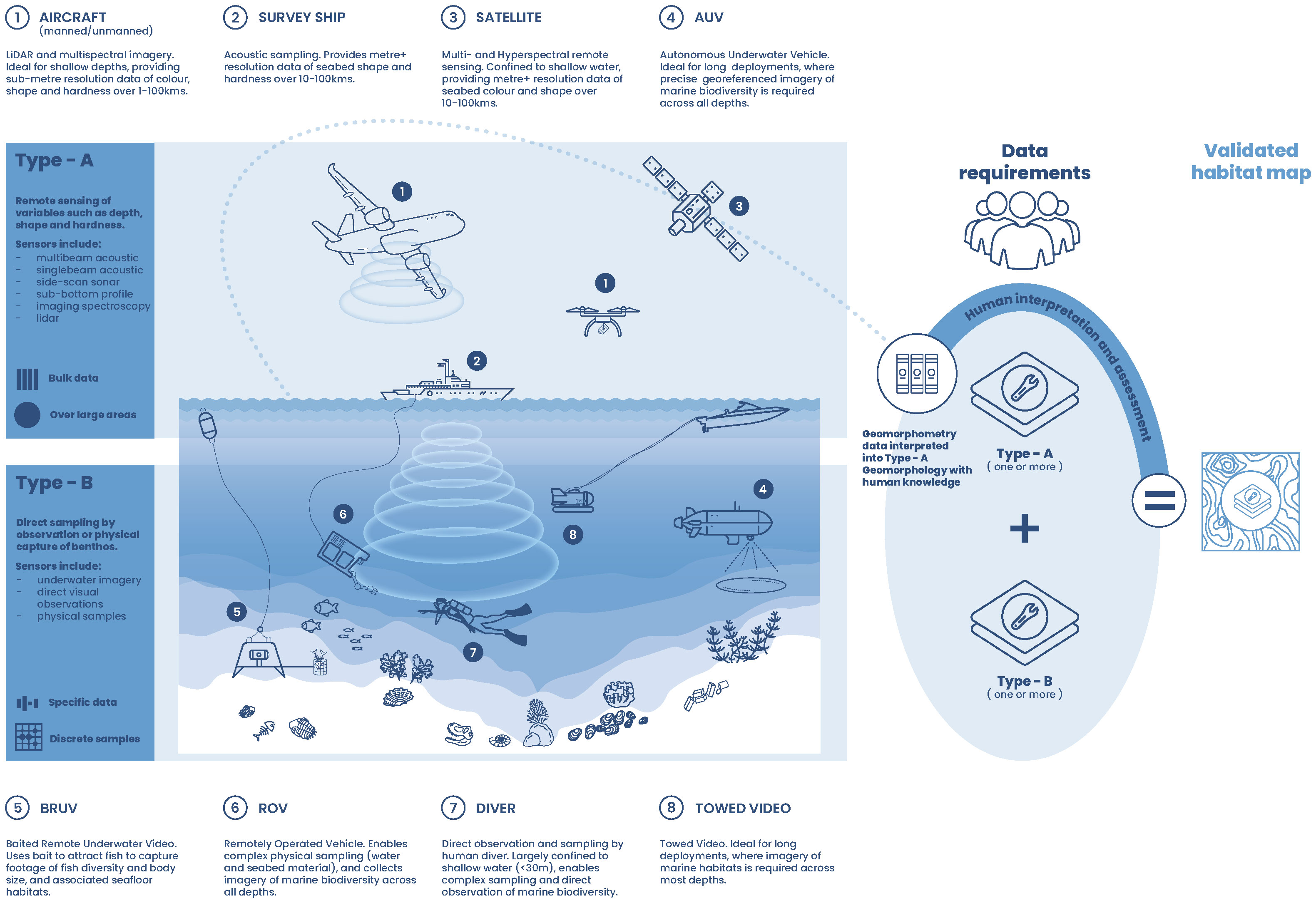
Figure 1 Type A data- represents remotely sensed collection of bathymetric data which can be used to create geomorphometry maps. Type B data- is ancillary data which is used to characterise the ecological habitats existing on the seafloor substrate. Both Type A and Type B data are required for the creation of a seafloor habitat map.

2 Materials and methods

2.1 Bathymetric data processing

Bathymetric survey data was collated in GeoTIFF format from the open data repositories AusSeabed and the Australian Ocean Data Network (see Supplementary Information 1 for a full list of collated datasets). The source surveys were conducted over varying temporal scales using different sonar techniques and were processed at a range of spatial resolutions (grid size). Bathymetry data was restricted to direct surveys (e.g., by acoustic techniques), with the exception of the Coral Sea, Central Eastern, Gifford, and Christmas Island AMPs where interpolated composite Digital Elevation Models (DEMs) were included, as these were characterised by large-scale features spanning a considerable depth range and benefited from the inclusion of ‘background’ data provided by DEMs. Each dataset was clipped to the boundaries of AMPs prior to processing. This was done using a polygon mask based on 2023 AMP boundaries supplied by the Department of Climate Change, Energy, the Environment and Water [last accessed Aug 2023]. Where required, data was resampled using bilinear method in the ArcMap tool (10.8.1) RESAMPLE. This was done to ensure gridding adequately covered of the surveyed region (i.e. no ‘speckly’ data). A raster catalog was created for each AMP (ArcMap (10.8.1) using the tool CREATE RASTER CATALOG). The catalogue was loaded with all intersecting clipped bathymetry GeoTIFFs, with source data ordered according to gridded resolution (i.e. fine scale data assigned a higher priority). Data was mosaiced into a single raster product for each AMP using the ArcMap tool RASTER CATALOG TO RASTER DATASET (options: Mosaic Operator: FIRST; Resampling Method: BILINEAR). This meant that, where bathymetry datasets overlapped in the mosaic, only the first (higher resolution) data was retained at each location. Mosaic datasets were then exported as GeoTIFF with lossless compression for subsequent morphological feature classification.

2.2 Geomorphometry classification

The morphological features for each AMP were calculated from the bathymetric surface of the seafloor using the geomorphon function in the Whitebox tools package (2.1.5) for R (4.2.1) (Jasiewicz and Stepinski, 2013). The specific search distances and slope thresholds were adjusted between AMPs depending on the data quality and resolution of bathymetry data and also on the particular characteristics of the seafloor (such as slope). This was done to reduce the effects of identified data artifacts that are known to impact seafloor variables derived from acoustic data (Lecours et al., 2017). All of the input parameters for each model for each AMP are provided as Supplementary Information (See Supplementary Information 2). Example code can be found here (https://github.com/jacquomo/Geomorphmetry_SeamapAus). Geomorphons were classified into morphological feature classes as identified in Dove et al. (2020) Seabed Morphology Features Glossary and exported as GeoTIFF for subsequent calculations.

2.3 Depth-based zonation

The ArcMap tool ZONAL STATISTICS AS TABLE was used to calculate the area covered by each geomorphometry class in each AMP using the rasters exported in step 2.2. The Australian Bathymetry and Topography Grid 250m (Whiteway, 2009) was used to generate vector masks of the eight depth zones specified in Parks Australia’s ME ‘common language’ (Hayes et al., 2021) (see https://seamapaustralia.org/map/#d120c916-fe99-474e-9d45-9e7b97e5ae36). Each AMP geomorphometry raster was clipped to the bounds of each depth mask, and ZONAL STATISTICS AS TABLE was performed again on depth-clipped datasets to obtain statistics on the area covered by each geomorphometry class, in each depth zone, for each AMP.

2.4 Summarising morphological characteristics of the AMPs

The R packages ggplot, ggdendro (4.2.1) were used to create the dendrogram, heatmap and the multidimensional scaling plots. In the dendrogram, the y-axis represents Ward’s distance, which is a measure of dissimilarity between clusters. The lower the Ward’s distance, the more similar the AMPs are in terms of morphological characteristics. The x-axis identifies individual AMPs. Each vertical line represents a cluster of AMPs, and the height of the line shows the distance at which they were joined. Shorter lines suggest that the AMPs in that cluster are more similar in terms of their morphological makeup, while longer lines suggest greater dissimilarity.

The heatmap function in R is a statistical tool that can be used to run a Euclidean distance clustering algorithm and produce the dendrogram. In the heatmap each row represents an AMP and each column represents a geomorphometry class. The colour intensity indicates the percentage of each geomorphometry class occurring in the AMP, with darker colours signifying higher occurrence. The cell values are the percentages of each geomorphometry class for the corresponding AMP. This representation shows that certain AMPs are dominated by specific morphological classes, while others are more diverse.

Multidimensional Scaling (MDS) is a technique used to reduce the dimensionality of data while preserving the pairwise distances between observations. Each point in the MDS plot represents an AMP, and the spatial arrangement of the points reflects the similarity or dissimilarity in morphological characteristics between them. Dimension 1 and Dimension 2: These are the two dimensions resulting from the MDS analysis. They are constructed in such a way that the pairwise distances between points in this 2D space approximate the pairwise distances in the original high-dimensional space as closely as possible. The closer the two points are in this space, the more similar their morphological makeup is. Conversely, the further away two points are from one another, the more dissimilar they are.

3 Results

The AMP estate is comprised of 61 AMPs represented across seven Networks around Australia (Figure 2). Heard Island and McDonald Islands is a 62^nd (non-AMP) reserve falling in the Australian marine jurisdiction and managed by the Australian Antarctic Division and was included in this analysis. Of these 62 AMPs, 37 were selected for geomorphometry assessment with the selection parameter being that bathymetric data coverage had to equal or exceed 25% of the total AMP area (see Supplementary Information 3). The 37 geomorphometry maps can be viewed as a single layer on the Seamap Australia data portal at https://seamapaustralia.org/map/#3064fc3f-b729-43cc-a8f1-cb071c49f759 [last accessed 20/09/2023], with accompanying bathymetry mosaics available at https://seamapaustralia.org/map/#1c0277fe-e922-417e-a589-0654232fa588 [last accessed 20/09/2023]. The following summary statistics selected for the analysis were identified as most crucial for making informed decisions regarding the improvement of monitoring and managing the AMP network.

Figure 2

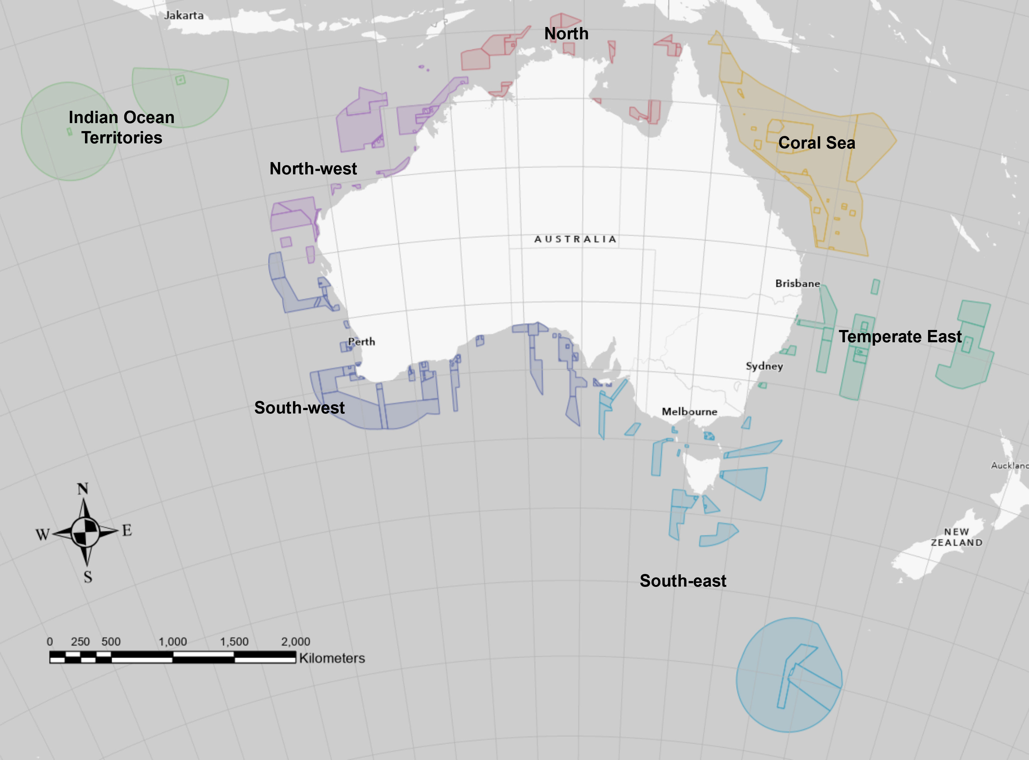
Figure 2 The Australian Marine Park (AMP) estate is comprised of 61 AMPs represented across seven Networks around Australia. See: https://seamapaustralia.org/map/#5d870854-90a9-4aa6-986b-81fb12da2680.

3.1 Summary of geomorphometric characteristics of the AMPs across all depth zones

Overall, when including DEMs, the mean bathymetry coverage in the AMPs across all depth zones was 57.8% (54.8% when excluding DEMs; Table 1). There are notable variations in bathymetry coverage across eight depth zones classified according to Parks Australia’s ME ‘common language’ (Hayes et al., 2021). For example, in the shallow (<30m), mesophotic (30-70m), rariphotic (70-200m) and abyssal (4,000-6,000m) depth zones the mean mapped percentage ranged from 40-59.3% (Table 1), indicating a modest mapping efforts in these regions. Conversely, the upper-slope (200-700m), mid-slope (700-2,000m) and lower-slope (2,000-4,000m) depth zones exhibited notably high mean mapped percentages, reaching 86.4%, 86.1% and 80.5%, respectively (Table 1).

Table 1

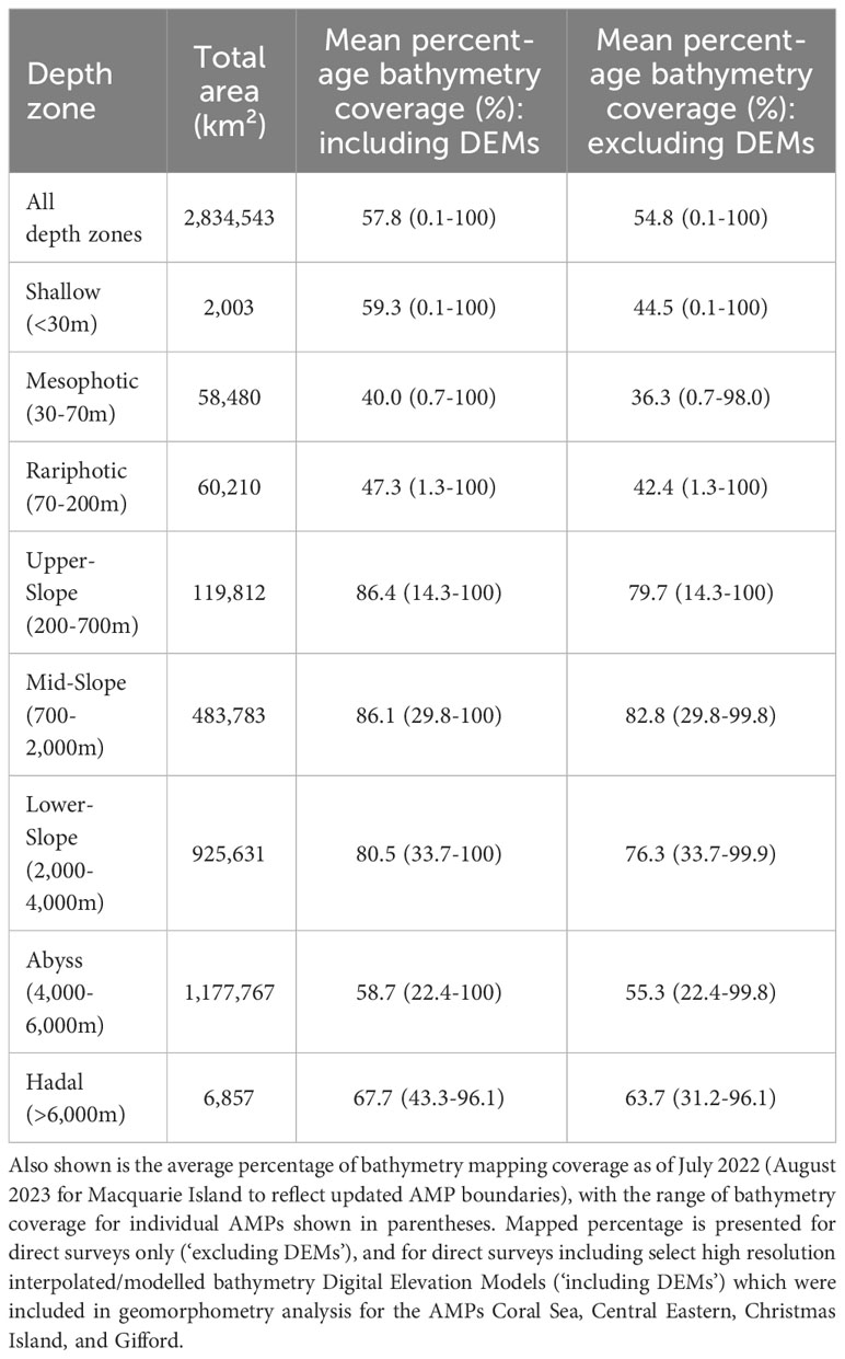
Table 1 Area occurring within each depth zone summed across the 36 Australian Marine Parks with sufficient bathymetry data (≥25% cover) for geomorphometry analysis (Heard and McDonald Islands excluded from depth analysis).

The most dominant geomorphometry class across all depths of the AMPs was the ‘Plane’ class, followed by ‘Slope’ (Figure 3). Across all AMPs combined, Plane comprised 58.4% of the geomorphometry classification, with Slope accounting for 18.2%. Apron, Saddle, and Valley were the next-most dominant classes, accounting for between 2 and 8% of total mapped coverage but were significantly less common than Plane and Slope.

Figure 3

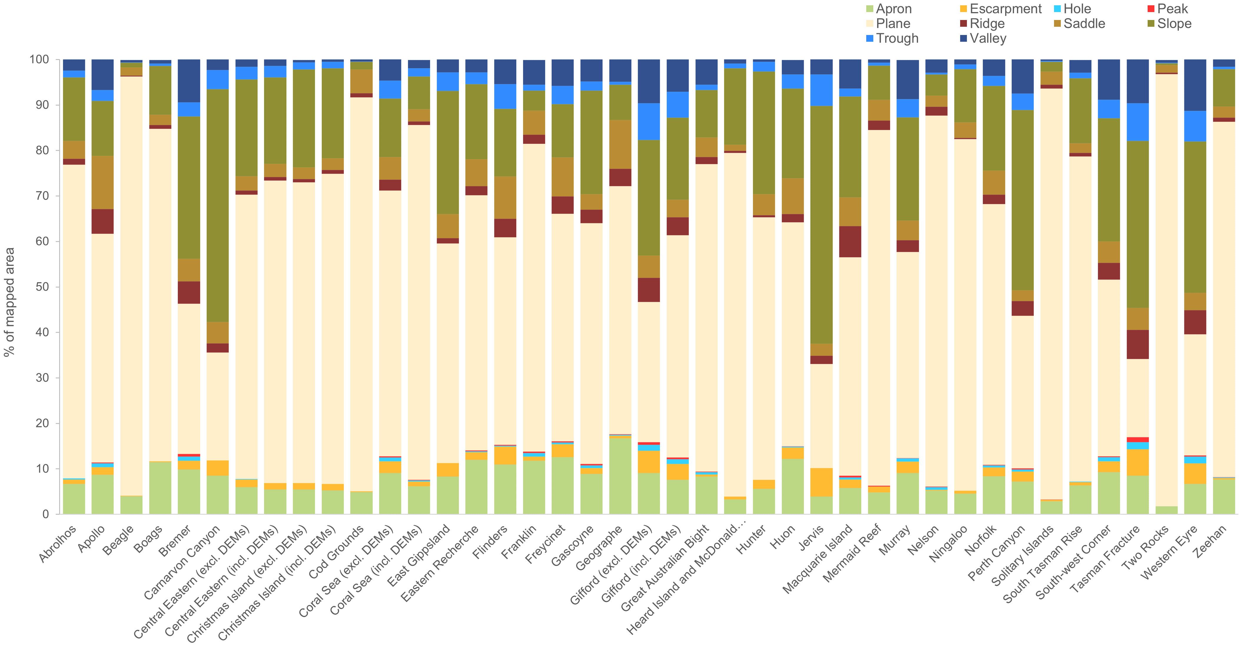
Figure 3 Stacked box plot showing the dominant geomorphometry class (% of mapped area) by Australian Marine Park.

3.1.1 Relationships between AMPs across all depths based on similarity in geomorphometry classes

The MDS scatterplot (Figure 4) provides a visual representation of how AMP Networks differ in their geomorphometric characteristics. The South-east and South-west Networks are at similar latitudes and have similar morphological profiles, being comprised of substantially less ‘Plane’ seafloor (45.3 and 42.7% for South-east and South-west Networks, respectively, versus 52.9-75.5% for all other Networks), and a relatively higher occurrence of Ridges (5.9 and 3.4%, versus 0.4-1.5%), Troughs (3.0 and 3.8% versus 1.1-2.5%), and Valleys (6.6 and 8.0% versus 0.5-4.7%). The Indian Ocean Territories Network stands alone, indicating that it has a unique set of morphological characteristics, different from all the other networks.

Figure 4

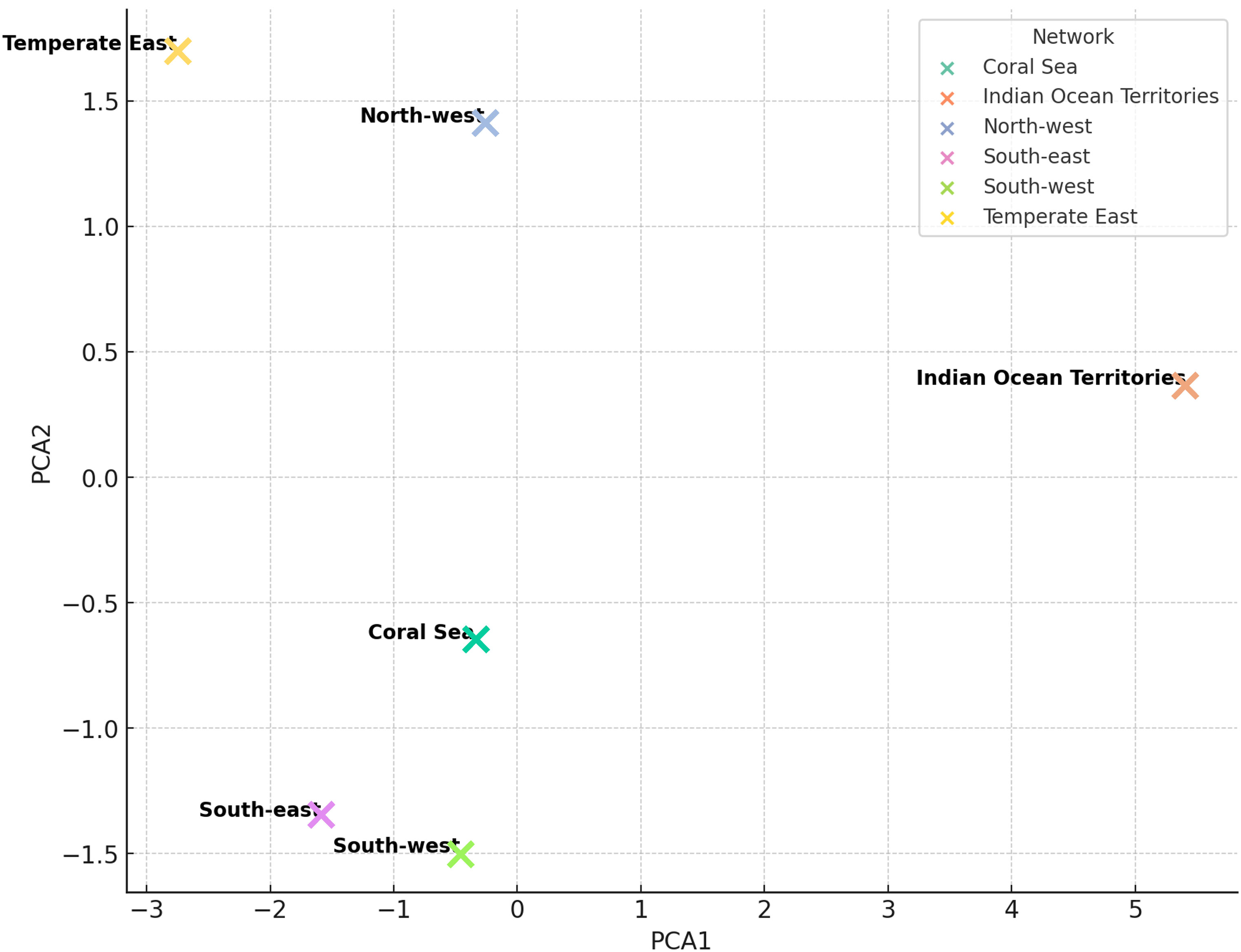
Figure 4 Multidimensional Scaling (MDS) plot illustrating similarities and differences in the seafloor morphological characteristics of Australian Marine Parks.

The hierarchical clustering dendrogram showed three primary clusters in AMPs based on their morphological characteristics across all depth zones (Figure 5). Interestingly, these clusters consisted of AMPs from multiple networks. For example, the first cluster consisted of six AMPs from the South-east network (South Tasman Rise, Boags, Franklin, Zeehan and Beagle), two from the South-west network (Abrolhos, Great Australian Bight), two from the North-west network (Mermaid Reef, Ningaloo), two from Temperate East (Cod grounds, Solitary Islands), the Coral Sea AMP and Heard Island and MacDonald Islands reserve. Further exploration of these patterns using a clustered heatmap (Figure 6) provides another avenue for visualising how morphological profiles vary between individual AMPs. This demonstrated that variations in the mapped extents of Plane and Slope geomorphometric classes were the primary drivers of these clusters (Figure 5). For example, Beagle and Solitary Islands, two AMPs from different Networks appearing in the same cluster (cluster #1; Figure 5) were comprised of Slope, Plain: 82%, 1% (Beagle) and 90%, 2% (Solitary Islands). In contrast, Carnarvon Canyon and Tasman Fracture in cluster #3, also from different Networks, were comprised of Slope, Plain: 24%, 51% (Carnarvon Canyon) and 17%, 37% (Tasman Fracture).

Figure 5

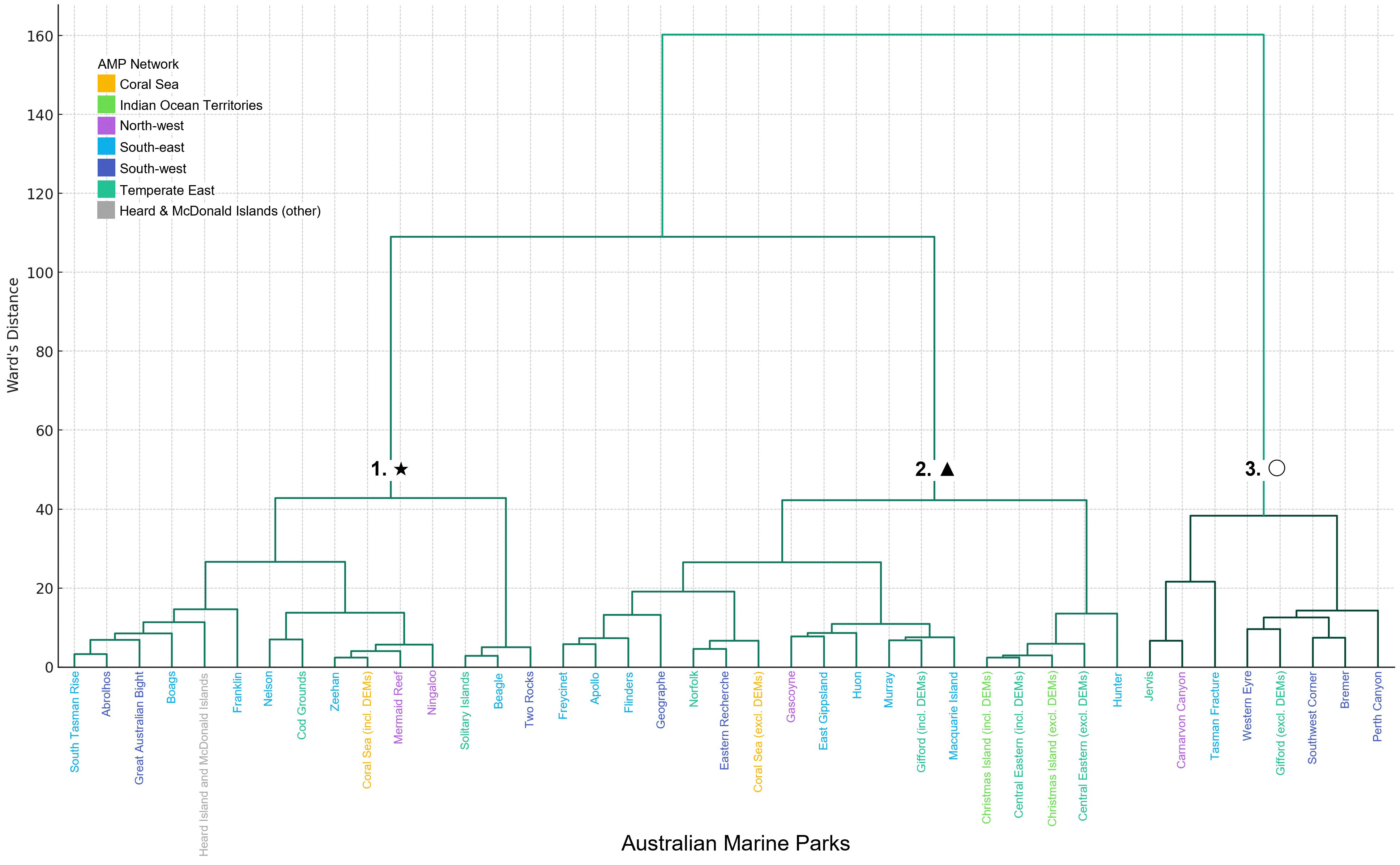
Figure 5 The hierarchical clustering dendrogram showed three primary clusters in AMPs based on their morphological characteristics across all depth zones. Symbols at branch stems indicate the three distinct clusters of AMPs.

Figure 6

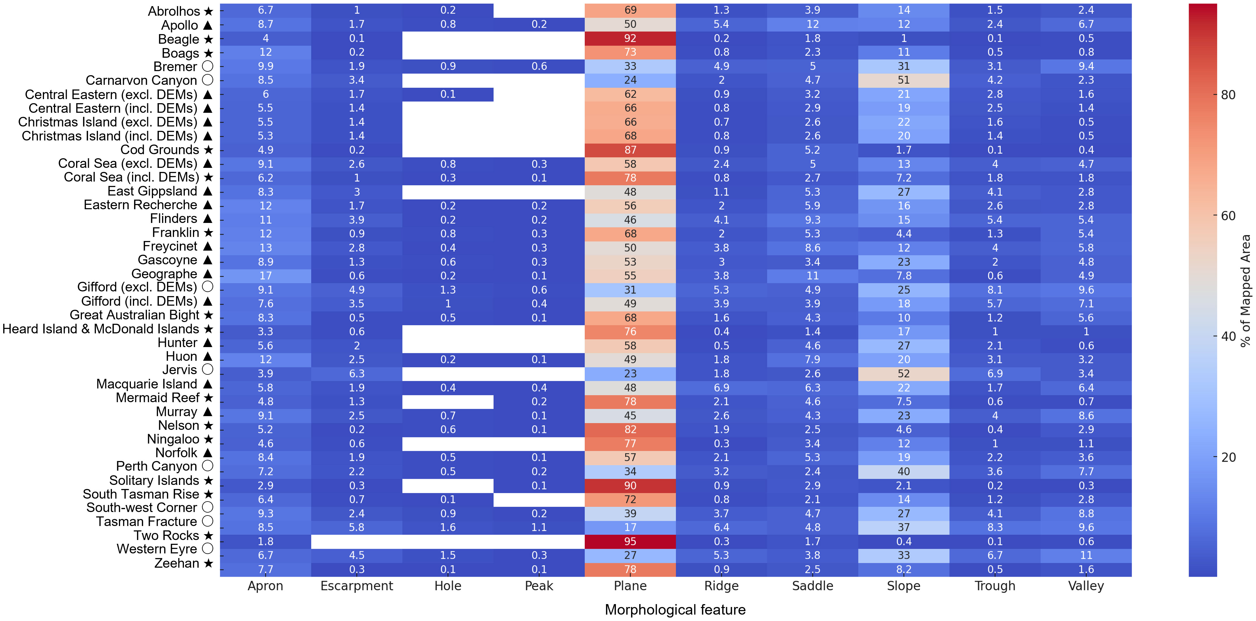
Figure 6 A tabular heatmap for comparing and contrasting the suite of seafloor morphological characteristics of individual AMPs. Morphological class is shown on the X-axis with AMPs on the Y-axis. Symbols adjacent to AMP names show clustering of AMPs as indicated in Figures 5 (dendrogram). Cell numbers indicate the % coverage of each morphological class as a fraction of the total mapped area.

3.2 Summary of geomorphometry characteristics of the AMPs by depth zones

The table in Supplementary Information 4 provides a comprehensive text summary of the depth and geomorphometry profile of each AMP for each of the eight depth zones. In the following section we explore how similarities and differences in these geomorphometry profiles varies between depth zones, using a MDS analysis. Results are presented for two selected depth zones: Mesophotic (<30-70 m) and Upper-Slope (200-700 m).

3.2.1 Geomorphometry characteristics of the Mesophotic (<30-70 m) depth zone

The mesophotic depth zone (30 – 70m) represents 2.1% of the total area of all analysed AMPs, of which 36% is mapped (40% including modelled data). MDS analysis revealed that eight of the AMPs exhibited morphological characteristics quite different to the other 16 AMPs with bathymetry mapping data in that depth zone (Figure 7). These 16 AMPs appear to be dominated by flat plane with small Slope and Apron features, for example Cod Grounds (https://seamapaustralia.org/map/#ec9b6aab-20ae-4dcb-ace6-5467a11eb4e0). In contrast, the eight other AMPs are dominated by higher-profile features such as Ridges and Peaks interspersed with Holes and Valleys, for example Franklin (https://seamapaustralia.org/map/#e73e1dbb-714b-4594-8e13-3885cea3bb77).

Figure 7

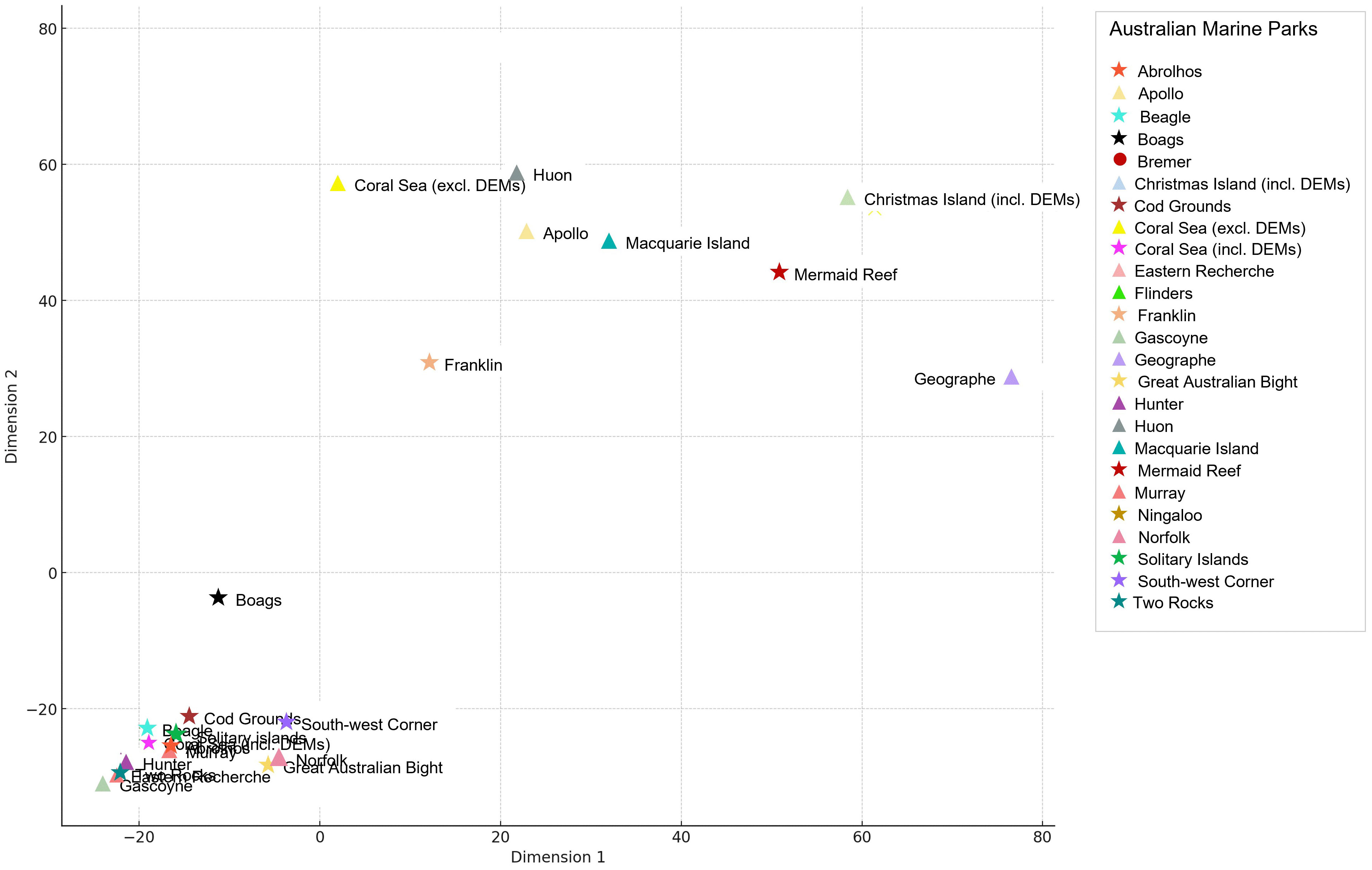
Figure 7 Multi-Dimensional Scaling (MDS) of the Australian Marine Parks based on their morphological characteristics in the Mesophotic depth range (30-70 m). Symbols match those used for Figures 5 and 6 showing the clustering indicated by all-depth dendrograms.

3.2.2 Morphological characteristics of the Upper-Slope (200 - 700 m) depth zone

The Upper-Slope depth zone (200 – 700 m) represents 4.2% of the total area of all analysed AMPs, of which 80% is mapped (86% including modelled data). The MDS plot (Figure 8) shows the points are broadly distributed across the plot, which implies a wide variation in geomorphometry features across different AMPs within this depth zone. In contrast to the plot for the Mesophotic zone which showed distinct clustering of AMPs sharing similar geomorphometric characteristics, in the Upper-Slope zone there are no clear groupings of AMPs with similar seafloor geomorphometry. For AMPs with a high proportion of their area falling within the Upper-Slope zone (e.g. Mermaid Reef; https://seamapaustralia.org/map/#4e653de6-31ff-4084-8359-25fbbb367b5c and Ningaloo; https://seamapaustralia.org/map/#5d612045-b9e1-43b0-9eb7-36f24aa08c6c), it may be necessary to develop customised management strategies tailored to their unique geomorphometry compositions.

Figure 8

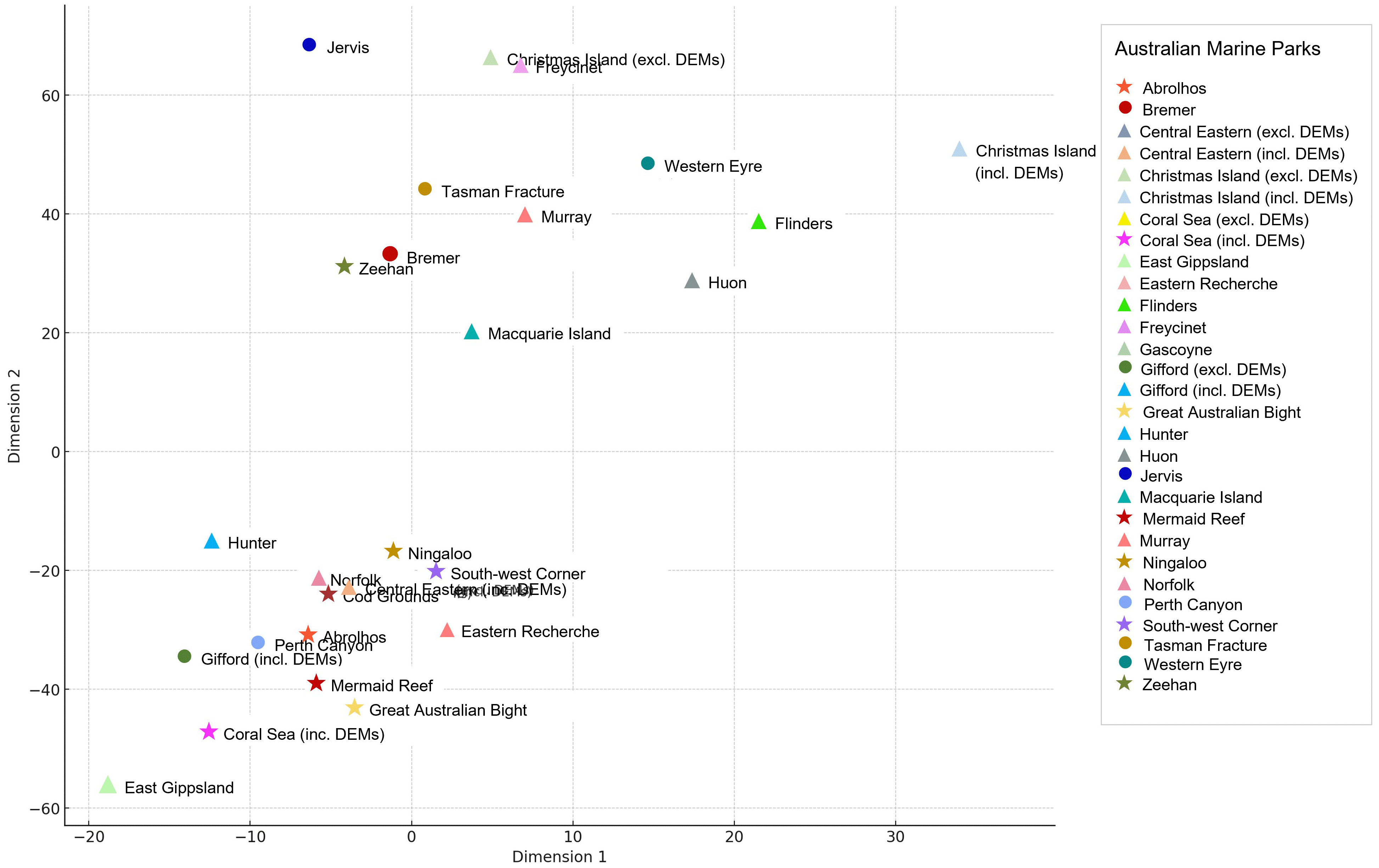
Figure 8 Multi-Dimensional Scaling (MDS) of the Australian Marine Parks based on their morphological characteristics in the Upper Slope depth range (200-700 m). Symbols match those used for Figures 5 and 6 showing the clustering indicated by all-depth dendrograms.

4 Discussion

Our approach identified similarities and differences in morphological features between AMPs within the same Network. In doing so, we identified unique or rare morphological classes across the AMP network. These results also permit rapid quantitative comparisons to be made between AMPs. Incorporating depth into the analysis allowed us to overcome the inherent biases arising from different depth characteristics across AMPs, allow a manager to quickly gauge which AMPs have similar morphological characteristics. This may allow the exchange of effective management strategies among similar AMPs, significantly boosting overall management efficiency. Furthermore, understanding the range of morphological features within specific depth zones of an AMP, in relation to existing knowledge of species and community distributions along these gradients, is vital. Linking morphological features with ecological data is critical for both habitat conservation and species protection. For example, the mesophotic (30-70 m) and rariphotic (70-150 m) zones, which are essential habitats for large fish (Bosch et al., 2021), often face substantial fishing pressure. Understanding the morphological composition of these depth zones, especially those impacted by anthropogenic pressures, can enhance our ability to monitor these species more effectively. This, in turn, is key to achieving better species protection and habitat conservation.

Defining the unique morphological features within specific AMPs can also aid in the development of tailored management and conservation strategies. For example, areas rich in certain features like ridges [which are known to be associated with high biodiversity (Monk et al., 2016)] or trenches (known to be important aggregation points) (Lörz et al., 2012) might need different management practices compared to flat seabed areas. However, it is important to recognise that characterising these features based on their morphology is only an initial step towards a deeper, more nuanced understanding of the seabed’s geomorphological dynamics and associated ecology. Common morphological features may be shaped by different geological and oceanographic processes. For example, structures like ridges and peaks may consist of current dominated soft sediment dunes or igneous bedrock outcrops, even sedimentary paleo shorelines, each associated with supporting different ecological communities (Brix et al., 2022).

The suite of analyses use here helps condense complex geomorphometry data into an easily interpretable form, providing valuable insights to underpin effective management. For example, the clustering AMPs based on the morphological features can be used to prioritise future field planning resource allocation, which in turn can provide evidence-based recommendations for park management. Furthermore, delineating the morphological features of an AMP can aid in the deployment of the most appropriate field-based techniques to collect ground-truthing seafloor data, a key step in progressing geomorphometry and geomorphology maps into validated benthic habitat maps (identified in Figure 1). Alternatively, if resources for monitoring or sampling are limited, the manager might focus on AMPs that are outliers in these plots, as they may have unique characteristics that may require special attention. Different morphological features may require different monitoring technologies and enforcement strategies, such as surveillance systems adapted to rugged terrain, steep seabed or deep valleys. Understanding the complexity of the seafloor in different water depths will also help to estimate the costs of further information gathering.

We acknowledge that the geomorphon approach taken here is limited to 10 classes which is substantially less than proposed in Dove et al. (2020). However, the strength of geomorphon approach is the ability to subjectively evaluate and quickly iterate (in seconds) on how well-aligned the mapped classes reflect the underlying topography. Noise artefacts in the underlying bathymetry mosaics (inherent in all acoustic data and reflective of the inclusive approach taken here with respect to input data) contributed to noise in the resulting morphological classification, and was particularly pronounced in deeper AMPs (e.g. offshore Macquarie Island, southern Tasman Fracture) where bathymetry data coverage was frequently derived from older surveys. Noise in bathymetry data presented as an increased artificial representation of ‘Valley’ and ‘Hole’ geomorphometry, as can be seen for Tasman Fracture, Western Eyre, South-west Corner and Murray AMPs in Figure 3 and at https://seamapaustralia.org/map/#b74070c4-1c69-47f8-bd75-b674859ad3a5. However, at a whole-of-AMP scale, noise had minimal effect on the representation of dominant and rare morphology feature classes, and in some cases the thresholds can be altered to reduce these inherent noise artifacts. The primary objective of this study was to develop a ‘toolkit’ for rapid, preliminary morphological analysis of national bathymetry holdings, offering managers a suite of statistical tools to enhance knowledge and improve management effectiveness of marine assets. Depending on the specific requirements of the analysis, particularly in terms of scale, it may be advisable to omit exceptionally ‘noisy’ or low-resolution data (refer to Supplementary Information 1 for a complete list of input datasets). A more selective approach would inevitably reduce spatial coverage but could enhance the accuracy and reliability of morphological classifications, especially at the level of individual classes.

This ability to quickly iterate using different thresholds and evaluate how well they align with the underlying bathymetric hillshade is not practical in approaches such as those proposed by(Arosio et al., 2023; Huang et al., 2023); which take hours to days to compute at the fine resolution of our current study and at the whole-of-AMP scale. We recognise that this flexibility may reduce the standardisation of geomorphometric classifications when applied across different datasets or AMPs. However, this adaptability is likely to enhance the accuracy of delineation of these classes within a specific AMP and, when applied cautiously, is a powerful technique. Regardless of the approach taken, geomorphometry maps are a highly visual spatial product, particularly when draped over bathymetry hillshade and viewed in combination with seafloor imagery and are invaluable for AMP stakeholder engagement communications. Geomorphometry is the first step in communicating the features present in a bathymetric data set and can aid in the understanding of certain management actions that are being taken, helping to highlight the ecological importance of a region. Managers emphasise the significance of being able to quantitatively categorise their AMP assets. This approach is enabled by the discrete labeling of geomorphometric features, whereas continuous bathymetry data does not offer the same capability beyond simple depth-based zonation. By integrating geomorphometric maps into the workflow as the first output to an AMPs survey, marine scientists and policymakers can make more informed decisions on the potential assets or values contained within their AMPs.

Whilst it is possible to track the use of different techniques used to extract morphological features about the seafloor as identified in various reviews (Lecours et al., 2016), it is much harder to assess their success in extracting morphological features consistently from bathymetric grids at different scales (Lecours et al., 2013), and within regions with incomplete coverage. Walbridge et al. (2018) present a workflow for benthic terrain modeler (BTM) that addresses the ‘call to arms’ over the rapidly increasing volume of high-resolution bathymetric data. The BTM method uses bathymetric data to enable simple characterisation of benthic biotic communities and geologic types and produces a collection of key morphological variables known to affect marine ecosystems and processes. Additionally, (Masetti et al., 2018) presented an approach that co-located bathymetry and backscatter to incorporate substratum type into geomophometry classes. However, the source bathymetric data used in our analysis consisted of 100s of surveys with varying grid resolution (from 0.3 to >200 m, sometimes occurring in a single AMP) and no available harmonised backscatter. We strongly encourage agencies that do acquire backscatter data to process it for this purpose of distinguishing hard versus soft substrata. It is not currently possible to infer substrata at an AMP scale using Australia’s publicly available backscatter data holdings and, importantly, it is important to have an approach that can deal with data that is ‘noisy’ or has varying gridded resolution. The model parameters using in our approach were altered to better capture the fine scale geomorphometry contained within the datasets (see Supplementary Information 1). When dealing with large datasets and batch processing techniques, Whitebox tools package for R (also available through QGIS) permitted the regeneration of consistent and rapid results enabling the researcher to iterate using difference parameters to select the best combination for that particular dataset. Furthermore, the added benefit of using Whitebox tools allows for the geomorphometric layers to be quickly updated as new data becomes available. The bathymetry data collation exercise undertaken in this study revealed that very few AMPs had comprehensive bathymetry mapping data across their entire depth range. Identifying and filling these data gaps could be a priority for future marine surveys and research.

5 Conclusion

Marine geomorphometry provides invaluable insights into the spatial and structural characteristics of the seafloor, playing a pivotal role in the effective management of the AMPestate. By providing a detailed inventory of a region’s geomorphometric features—such as slopes, ridges, and valleys—geomorphometry enables park managers to make informed decisions on conservation strategies, resource allocation, and monitoring programs.

The use of advanced analytical techniques like Multidimensional Scaling (MDS) and cluster analysis enhance our understanding of the unique and common characteristics of different AMPs. These techniques can also help identify which AMPs may require tailored management strategies, particularly in specific depth zones like the Mesophotic and Lower-Slope.

However, it is important to acknowledge some limitations of this approach. Firstly, the quality of geomorphometric output is dependent on the resolution and accuracy of source bathymetric survey and Digital Elevation Model data (if included). Low-resolution data can result in an incomplete or misleading picture of the morphological features present and can be complicated to interpret alongside neighbouring high-resolution data. Secondly, the interpretation of reduced-dimensionality plots, like dendrograms and MDS, requires expertise, and the axes are not always straightforward to interpret. Lastly, while average mapped coverage can provide a general idea of the depth zones that are well-studied, it doesn’t provide a complete picture of the spatial variability within each AMP due to the extent of the data gaps across the AMP network and may skew some of the results (for example, if previous sampling has targeted a particular depth range that is only represented in some AMPs). Marine geomorphometry data serves as a preliminary analysis tool for AMP management but should be used with other data sources and expert judgment to provide a comprehensive and nuanced understanding of critical marine environments. This study initiates and makes preliminary recommendations for systematically applying this approach to AMP management. However, development of a comprehensive toolkit would simplify a broader implementation.

Geomorphometric maps play a role in improving the integrated monitoring and management of marine ecosystems through improved monitoring for a) habitat identification, b) baseline data, and c) data integration. There is a clear demand within the seafloor mapping community for standardised morphological and (where available) geomorphological practices to ensure consistency in mapping the AMPs benthic assets across the vast marine estate. We propose the adoption of a standardised classification model as the first step in interpreting multibeam data collected within the AMP network. This approach would not only facilitate comparisons of seafloor assets across different AMP regions but also serve as a valuable preliminary information source for survey planning. In the process of converting bathymetric datasets into benthic habitat maps, the procedure of consistently identifying morphological features would enhance how surveys are planned and allow direct observational sampling to target representative morphologies ensuring that habitat validation data is equally weighted to morphological proxies underpinning benthic habitat maps.

Data availability statement

The datasets presented in this study can be found in online repositories. The names of the repository/repositories and accession number(s) can be found in the article/Supplementary Material.

Author contributions

VL: Conceptualization, Data curation, Formal Analysis, Funding acquisition, Investigation, Methodology, Project administration, Resources, Writing – original draft, Writing – review & editing. EF: Data curation, Formal Analysis, Investigation, Methodology, Validation, Writing – original draft, Writing – review & editing. JM: Conceptualization, Data curation, Formal Analysis, Investigation, Methodology, Writing – original draft, Writing – review & editing. PW: Conceptualization, Project administration, Resources, Writing – review & editing.

Funding

The author(s) declare financial support was received for the research, authorship, and/or publication of this article. This research was completed with funding from the "Our Marine Park grant scheme" 'Extending seabed horizons: Seamap Australia tools and analytics for marine park managers’ Department of Environment and Energy (Commonwealth), the Institute of Marine and Antarctic Studies at the University of Tasmania and the Australian Government under the National Environmental Science Program.

Conflict of interest

The authors declare that the research was conducted in the absence of any commercial or financial relationships that could be construed as a potential conflict of interest.

Publisher’s note

All claims expressed in this article are solely those of the authors and do not necessarily represent those of their affiliated organizations, or those of the publisher, the editors and the reviewers. Any product that may be evaluated in this article, or claim that may be made by its manufacturer, is not guaranteed or endorsed by the publisher.

Supplementary material

The Supplementary Material for this article can be found online at: https://www.frontiersin.org/articles/10.3389/fmars.2023.1302108/full#supplementary-material

References

Arosio R., Wheeler A. J., Sacchetti F., Guinan J., Benetti S., O’Keeffe E., et al. (2023). “The geomorphology of Ireland’s continental shelf”. J. Maps 19 (1), 2283192. doi: 10.1080/17445647.2023.2283192

CrossRef Full Text | Google Scholar

Bosch N., Monk J., Goetze N., Wilson S., Babcock R., Barrett N., et al. (2021). Effects of human footprint and biophysical factors on the body-size structure of fished marine species. Conserv. Biol. 36, e13807. doi: 10.1111/cobi.13807

PubMed Abstract | CrossRef Full Text | Google Scholar

Brix S., Kaiser S., Lörz A.-N., Le Saout M., Schumacher M., Bonk F., et al. (2022). Habitat variability and faunal zonation at the Ægir Ridge, a canyon-like structure in the deep Norwegian Sea. PeerJ 10, e13394. doi: 10.7717/peerj.13394

PubMed Abstract | CrossRef Full Text | Google Scholar

Butler C., Lucieer V., Walsh P., Flukes E., Johnson C. (2017). Seamap Australia (Version 1.0) the development of a national marine classification scheme for the Australian continental shelf. Final report to the Australian Online Data Network (AODN) (Hobart, Tasmania Australia: University of Tasmania). 52pp.

Google Scholar

Clark M. R., Watling L., Rowden A. A., Guinotte J. M., Smith C. R. (2011). A global seamount classification to aid the scientific design of marine protected area networks. Ocean Coast. Manage. 54 (1), 19–36. doi: 10.1016/j.ocecoaman.2010.10.006

CrossRef Full Text | Google Scholar

Cogan C. B., Todd B. J., Lawton P., Noji T. T. (2009). The role of marine habitat mapping in ecosystem-based management. Ices J. Mar. Sci. 66 (9), 2033–2042. doi: 10.1093/icesjms/fsp214

CrossRef Full Text | Google Scholar

Colenutt A., Mason T., Cocuccio A., Kinnear R., Parker D. (2013). Nearshore substrate and marine habitat mapping to inform marine policy and coastal management. J. Coast. Res. 65 (sp2), 1509–1514. doi: 10.2112/SI65-255.1

CrossRef Full Text | Google Scholar

Commonwealth Environmental Water (2013). Monitoring, Evaluation, Reporting and Improvement Framework. V2.0. (Commonwealth Environmental Water) Available at: extension://efaidnbmnnnibpcajpcglclefindmkaj/https://www.dcceew.gov.au/sites/default/files/documents/meri-framework_1.pdf.

Google Scholar

Diesing M., Mitchell P. J., O’Keeffe E., Gavazzi G. O. A. M., Bas T. L. (2020). Limitations of predicting substrate classes on a sedimentary complex but morphologically simple seabed. Remote Sens. 12 (20), 3398. doi: 10.3390/rs12203398

CrossRef Full Text | Google Scholar

Dove D., Nanson R., Bjarnadóttir L. R., Guinan J., Gafeira J., Post A., et al. (2020). A two-part seabed geomorphology classification scheme: (v.2), British Geological Survey: 22.

Google Scholar

Furlan E., Torresan S., Ronco P., Critto A., Breil M., Kontogianni A., et al. (2018). Tools and methods to support adaptive policy making in marine areas: Review and implementation of the Adaptive Marine Policy Toolbox. Ocean Coast. Manage. 151, 25–35. doi: 10.1016/j.ocecoaman.2017.10.029

CrossRef Full Text | Google Scholar

Harris P., Macmillan-Lawler M., Rupp J., Baker E. (2014). Geomorphology of the oceans. Mar. Geol. 352, 4–24. doi: 10.1016/j.margeo.2014.01.011

CrossRef Full Text | Google Scholar

Harris P. T., Baker E. K. (2012). Seafloor Geomorphology as Benthic Habitat: GeoHab Atlas of seafloor geomorphic features and benthic habitats (Germany: Elsevier Science).

Google Scholar

Hayes K. R., Dunstan P., Woolley S., Barrett N., Howe S. A., Samson C. R., et al. (2021). Designing a Targeted Monitoring Program to Support Evidence Based Management of Australian Marine Parks: A Pilot on the South-East Marine Parks Network. Report to Parks Australia and the National Environmental Science Program (Hobart, Australia., University of Tasmanian and CSIRO: Marine Biodiversity Hub. Parks Australia).

Google Scholar

Huang Z., Nanson R., McNeil M., Wenderlich M., Gafeira J., Post A., et al. (2023). Rule-based semi-automated tools for mapping seabed morphology from bathymetry data. Front. Mar. Sci. 10. doi: 10.3389/fmars.2023.1236788

CrossRef Full Text | Google Scholar

Jasiewicz J., Stepinski T. (2013). Geomorphons — a pattern recognition approach to classification and mapping of landforms. Geomorphology 182, 147–156. doi: 10.1016/j.geomorph.2012.11.005

CrossRef Full Text | Google Scholar

Lecours V., Devillers R., Edinger E. N., Brown C. J., Lucieer V. L. (2017). Influence of artefacts in marine digital terrain models on habitat maps and species distribution models: a multiscale assessment. Remote Sens. Ecol. Conserv. 3 (4), 232–246. doi: 10.1002/rse2.49

CrossRef Full Text | Google Scholar

Lecours V., Devilliers R., Edinger E. N., Brown C. J., Lucieer V. L. (2013). “Exploring the role spatial scale plays in marine habitat mapping using multiscale geomorphometric analyses,” in Geohab Marine Geological and Biological Habitat Mapping Conference 2013, F. Andrea. Rome, Italy. 1–17 (Italian Geological Society).

Google Scholar

Lecours V., Dolan M. F. J., Micallef A., Lucieer V. L. (2016). A review of marine geomorphometry, the quantitative study of the seafloor. Hydrol. Earth Syst. Sci. 20 (8), 3207–3244. doi: 10.5194/hess-20-3207-2016

CrossRef Full Text | Google Scholar

Lecours V., Lucieer V., Dolan M., Micallef A. (2018). Recent and future trends in marine geomorphometry. Geomorphom. 2018. Colorado United States PeerJ. 8, 1–4.

Google Scholar

Lörz A. N., Berkenbusch K., Nodder S., Ahyong S., Bowden D., McMillan P., et al. (2012). A review of deep-sea benthic biodiversity associated with trench, canyon and abyssal habitats below 1500 m depth in New Zealand waters. N. Zealand Aquatic Environ. Biodiversity Rep. Rep. N. Zealand pp.133.

Google Scholar

Lucieer V. L., Hill N., Barrett N. S., Nichol S. (2013). Do marine substrates ‘look’ and ‘sound’ the same? Supervised classification of multibeam acoustic data using autonomous underwater vehicle images. Estuarine Coast. Shelf Sci. 117, 94–106. doi: 10.1016/j.ecss.2012.11.001

CrossRef Full Text | Google Scholar

Lucieer V., Lecours V., Dolan M. F. J. (2018). Charting the course for future developments in marine geomorphometry: an introduction to the special issue. Geosciences 8 (12), 1–9. doi: 10.3390/geosciences8120477

CrossRef Full Text | Google Scholar

Lucieer V. L., Lecours V., Dolan M. J. F. (2019). Marine geomorphometry: geosciences special issue. Mar. Geomorphom., 1–402. doi: 10.3390/books978-3-03897-955-5

CrossRef Full Text | Google Scholar

Masetti G., Mayer L. A., Ward L. G. (2018). A bathymetry- and reflectivity-based approach for seafloor segmentation. Geosciences 8, 14. doi: 10.3390/geosciences8010014

CrossRef Full Text | Google Scholar

McArthur M. A., Brooke P. B., Przeslawski R., Ryan D. A., Lucieer V. L., Nichol S., et al. (2010). On the use of abiotic surrogates to describe marine benthic biodiversity. Estuarine Coast. Shelf Sci. 88 (1), 21–32. doi: 10.1016/j.ecss.2010.03.003

CrossRef Full Text | Google Scholar

Micallef A., Lecours V., Dolan M., Lucieer V. (2016). “Marine geomorphometry: overview and opportunities,” in EGU General Assembly 2016, (Vienna, Austria: Copernicus GmbH), 18, 6264.

Google Scholar

Monk J., Barrett N. S., Hill N. A., Lucieer V. L., Nichol S. L., Siwabessy P. J. W., et al. (2016). Outcropping reef ledges drive patterns of epibenthic assemblage diversity on cross-shelf habitats. Biodivers. Conserv. 25 (3), 485–502. doi: 10.1007/s10531-016-1058-1

CrossRef Full Text | Google Scholar

Monk J., Williams J., Barrett N. S., Jordan A. R., Lucieer V. L., Althaus F., et al. (2017). Biological and habitat feature descriptions for the continental shelves of Australia’s temperate-water marine parks- including collation of existing mapping in all AMPs (Hobart, Tasmania, Australia: Institute for Marine and Antarctic Studies, UTAS), 313.

Google Scholar

Pike R. J. (2000). Geomorphometry - diversity in quantitative surface analysis. Prog. Phys. Geogr. 24 (1), 1–20. doi: 10.1177/030913330002400101

CrossRef Full Text | Google Scholar

Strong J. A., Clements A., Lillis H., Galparsoro I., Bildstein T., Pesch R. (2018). A review of the influence of marine habitat classification schemes on mapping studies: inherent assumptions, influence on end products, and suggestions for future developments. ICES J. Mar. Sci. 76 (1), 10–22. doi: 10.1093/icesjms/fsy161

CrossRef Full Text | Google Scholar

Walbridge S., Slocum N., Pobuda M., Wright D. (2018). Unified geomorphological analysis workflows with benthic terrain modeler. Geosciences 8 (3), 94. doi: 10.3390/geosciences8030094

CrossRef Full Text | Google Scholar

Whiteway T. (2009). Australian bathymetry and topography grid. Geosci. Aust. doi: 10.4225/25/53D99B6581B9A

CrossRef Full Text | Google Scholar

Wyborn C., Evans M. C. (2021). Conservation needs to break free from global priority mapping. Nat. Ecol. Evol. 5 (10), 1322–1324. doi: 10.1038/s41559-021-01540-x

PubMed Abstract | CrossRef Full Text | Google Scholar