Research on underwater acoustic field prediction method based on physics-informed neural network

In the field of underwater acoustic field prediction, numerical simulation methods and machine learning techniques are two commonly used methods. However, the numerical simulation method requires grid division. The machine learning method can only sometimes analyze the physical significance of the model. To address these problems, this paper proposes an underwater acoustic field prediction method based on a physics-informed neural network (UAFP-PINN). Firstly, a loss function incorporating physical constraints is introduced, incorporating the Helmholtz equation that describes the characteristics of the underwater acoustic field. This loss function is a foundation for establishing the underwater acoustic field prediction model using a physics-informed neural network. The model takes the coordinate information of the acoustic field point as input and employs a fully connected deep neural network to output the predicted values of the coordinates. The predicted value is refined using the loss function with physical information, ensuring the trained model possesses clear physical significance. Finally, the proposed prediction model is analyzed and validated in two dimensions: the two-dimensional acoustic field and the three-dimensional acoustic field. The results show that the mean square error between the prediction and simulation values of the two-dimensional model is only 0.01. The proposed model can effectively predict the distribution of the two-dimensional underwater sound field, and the model can also predict the sound field in the three-dimensional space.

1 Introduction

High-precision underwater acoustic field model is of great significance for underwater acoustic communication, sonar effectiveness evaluation, underwater target recognition and location, etc. Establishing a high-precision underwater acoustic field prediction model is one of the important research contents in underwater acoustic field. For example, the establishment of highly accurate underwater acoustic field can help synthetic aperture sonar (SAS) to obtain higher resolution sonar images. Zhang (2023) proposed a new method to simulate the original SAS echo. The transmitted signal was Fourier transformed and multiplied by the phase shift of the delay, and the spectrum of the echo signal was accurately obtained. Yang et al. (2023) proposed a multi-receiver SAS imaging algorithm based on Loffeld Bistatic formula (LBF). Zhang et al. (2021) proposed a multi-receiver SAS image processing method and proved that under certain conditions, the bistable formula of Loffeld can be simplified to the same formula as the spectrum based on phase center approximation. Zhang et al. (2023) proposed a SAS imaging algorithm by rerepresenting the Loffeld bistable formula (LBF), which includes quasi-monostable (QM) and multi-receiver deformed (MD) phases, as range-variant phase and range-invariant phase. In the process of SAS signal transmission, there will be attenuation, and the establishment of high-precision underwater acoustic field can compensate the attenuation signal accordingly. At present,the numerical simulation and the machine learning are common methods to forecast the underwater acoustic field. The numerical simulation method mainly uses ray method, normal mode method, parabola method, beam integration method (Belibassakis et al., 2014) to establish physical models and calculate underwater acoustic field. Kiryanov et al. (2015) established a random non-uniform wave field model for evaluating sound velocity field based on the results of deep-sea acoustic long-range propagation test. Miller (1954) introduced the coupled mode to extend the solution range of the differential equation to the number of waveguides dependent on the distance. For the normal mode method, the finite element method is usually used to build the acoustic field model, and the KRAKEN model is widely used to build the acoustic field by finite element as a representative model. Zhou and Luo (2021) established a finite element model for predicting underwater acoustic field based on Cartesian coordinate system in a two-dimensional environment, whose universality is better than that of KRAKEN model. Teng et al. (2010) used the boundary element method to simulate the acoustic field around two kinds of underwater communication transducers, and the prediction results are generally applicable. The spectral method is a high precision method for solving differential equations, and it also plays an important role in promoting the calculation of underwater acoustic field. Tu et al. (2022) used spectral method and coupled modes to solve the acoustic field of underwater linear source. In this paper, Chebyshev-Tau spectral method was used to solve the horizontal wave number of irrelevant segments in the approximate range, and a global matrix was constructed to solve the coupling coefficient of the acoustic field and synthesize the complete acoustic field. Tu et al. (2021) used Chebyshev-Tau spectral method to construct the normal mode model of underwater acoustic field, and converted the relevant differential equations into a complex matrix eigenvalue problem formed by orthogonal basis with Chebyshev polynomials to solve the horizontal beam. Tu et al. (2020) used Chebyshev-Tau spectral method to solve the normal mode model and parabolic equation, and the solution accuracy was higher than that of the finite element method. Although the numerical simulation method can directly forecast the underwater acoustic field by using the physical rules, the numerical solution often needs to divide the regular grid to simplify the model calculation, and it is difficult to predict the acoustic field model with irregular boundaries. With the development of computer hardware, the neural network, which is one of the important methods in machine learning, has been used more and more to predict underwater acoustic field. Ahmed et al. (2021) established a machine learning model to predict the sound velocity profile in deep water and shallow water. The accuracy of this model reached 99.99% and the prediction effect was better than the acoustic field model forecasted by the equation. Based on the self-defined loss function, He et al. (2022) constructed a single output joint neural network and a multi-output neural network with physical constraints to accurately forecast the beam and feature function of the underwater acoustic field.

Machine learning method has greatly improved the accuracy of underwater acoustic field prediction, but there are some obvious problems. First of all, the model trained by the neural network does not have a clear physical meaning, and it has poor adaptability to different environments. Secondly, the neural network needs a large amount of historical data as support to ensure that the trained model has a high accuracy. Figure 1 (Karniadakis et al., 2021) shows the relationship between data volume and physical parameters in the model prediction problem. In case 1, assuming clear physical laws and boundary conditions are known, the corresponding problem can be solved according to physical rules. In this case, the numerical simulation method can be used to predict the underwater acoustic field. In case 2, only a large amount of data is known but the specific physical rules are not clear, and machine learning can be used to predict the acoustic field problem. The real underwater acoustic field prediction is a problem in case 3: there are sufficient data but some parameters in the physical rules are not clear, which cannot be solved directly by the physical rules.

FIGURE 1

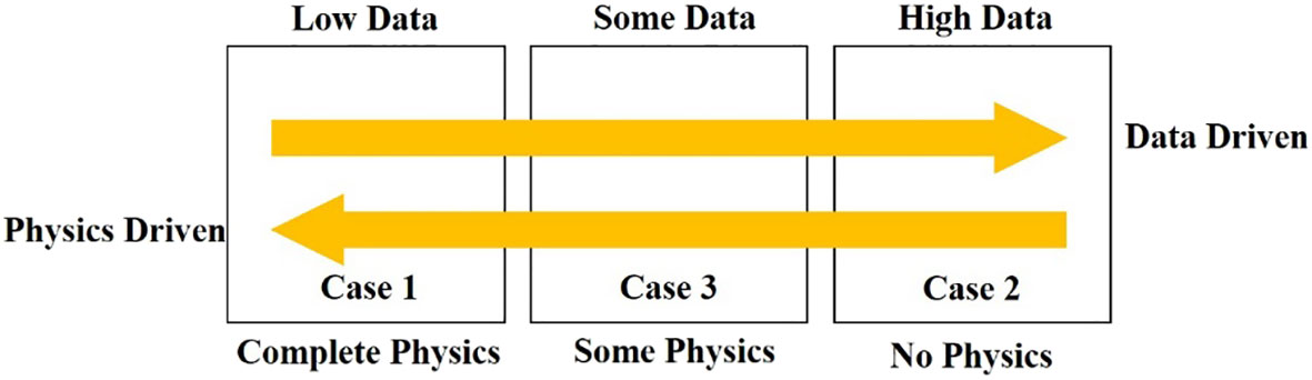
Figure 1 The relationship between data volume and physical rules.

Physics-informed neural network (PINN) is a new kind of neural network, which is used to solve the problem of case 3 in Figure 1. It essentially trains the neural network with physical equations as constraints, so that the prediction model can meet certain physical rules. The method has been applied to geophysics, fluid mechanics, plasma dynamics, high dimensional system problems, quantum chemistry, materials science and other fields closely related to physics. Zhu et al. (2021) introduced a deep learning framework for inversion of seismic data. This paper combined DNN and numerical partial differential equation solvers to solve problems such as seismic wave velocity estimation, fault rupture imaging, seismic location and source time function inversion. Raissi et al. (2019) combined Navier-Stokes equations with deep learning to build a model based on physics-informed neural network and predict pressure distributions in incompressible fluids. Shukla et al. (2020) used physics-informed neural network to detect cracks on the surface of materials, designed a trained PINN to solve the problem of identification and characterization of cracks on the surface of metal plates, and solved the acoustic wave equation using measured ultrasonic surface acoustic wave data with a frequency of 5 MHz. Wu et al. (2022) introduced the Helmholtz equation and its corresponding boundary conditions into neural networks to establish physics-informed neural networks describing acoustic problems. These neural network algorithms can not only reflect the distribution of training data samples, but also follow the physical laws described by partial differential equations. Pfau et al. (2020) combined the wave function of Fermi-Dirac statistics with deep learning networks to calculate the solution of the multi-electron Schrodinger equation. Rotskoff et al. (2022) used PINN method to solve the high-dimensional problem and gave the results of the probability distribution in the 144-dimensional Allen-Cahn type system, indicating that the method is effective for high-dimensional systems, but its adaptability needs to be optimized for more complex systems. Zhang et al. (2022) used deep neural network to modify the displacement factor of surrounding rock of Verruijt-Booker solution, and constructed the correlation between the surface settlement and the spatial position of tunnel excavation face. Then, the physics equations of the corrected solutions were used to construct PINN, and the results were better than those of DNN alone. Zou et al. (2023) designed a PINN model to solve the seismic wave equation. Du et al. (2023) used the three-dimensional function equation and other physical rules to form a loss function, and trained the neural network by minimizing the loss function. The final output satisfied the function equation and the result was better than the traditional calculation result.

In the underwater acoustic field, wave theory is usually used to describe underwater acoustic propagation. In this paper, the underwater sound propagation equation is derived based the framework of wave theory, which is used as constraint to train the deep neural network, and finally the underwater acoustic field prediction model with practical physical significance is obtained. The specific arrangement of this paper is as follows:

1) Deriving the Helmholtz equation of underwater acoustic propagation in homogeneous medium and establishing the model of underwater acoustic propagation based on the Helmholtz equation.

2) Designing a fully connected deep neural network. Introducing Helmholtz equation into the training process of neural network. Establishing a physics-informed neural network based on the Helmholtz equation.

3) Adjusting different training parameters of neural network, analyzing model training efficiency and prediction accuracy, and finding the best network design parameters.

The rest of the paper is organized as follows: in Chapter 2, the Helmholtz equation describing the distribution of sound pressure in underwater acoustic field is derived. In Chapter 3, the structure of underwater acoustic field prediction physics-informed neural network (UAFP-PINN) is described in detail. In Chapter 4, UAFP-PINN is used to forecast the 2D and 3D underwater acoustic fields, and the prediction results are analyzed in detail. Finally, the conclusion and summary is mentioned in Chapter 5.

2 Theory

2.1 Helmholtz equation

Wave theory is a strict mathematical method, which can be used to derive the Helmholtz equation describing the law of underwater sound propagation. For ideal fluids, the wave equation for sound pressure can be written as follows (Jensen et al., 2011):

$\begin{array}{ll}\rho \nabla ·(\frac{1}{\rho }\nabla p)-\frac{1}{c^2}\frac{{\partial }^{2}p}{\partial t^2}=0& (1)\end{array}$

In the above formula, $p$ is the sound pressure value of the acoustic field, $\rho$ is the density of the medium, $c$ is the speed of sound in the medium, and both density and speed of sound are functions of space and time. $\nabla$ is a Hamiltonian operator. To simplify the calculation, assuming that the density does not vary with space (Jensen et al., 2011), Formula 1 can be simplified to the following formula:

$\begin{array}{ll}{\nabla }^{2}p-\frac{1}{c^2}\frac{{\partial }^{2}p}{\partial t^2}=0& (2)\end{array}$

Formula 2 is the wave equation in a homogeneous medium, which can be approximated to the ocean acoustic field in a homogeneous medium for a smaller scale ocean acoustic field model. ${\nabla }^2$ stands for Laplace operator. For simple harmonic wave, $\frac{{\partial }^2}{\partial t^2}=-{\omega }^2$, $\omega$ is radiant frequency, introducing the potential function $\Psi =\frac{p}{\sqrt{\rho }}$, Formula 2 can be written as the following formula (Liu et al., 2019):

$\begin{array}{ll}{\nabla }^2\Psi +k^2(x,y,z)\Psi =0 & (3)\end{array}$

In Formula 3, $\Psi$ is the potential function, $k$ is the wave number in the medium, which is calculated by the formula $k=\frac{\omega }{c}$. The density in a uniform medium is a constant, and it can be seen from the potential function formula that there is a linear relationship between the sound pressure and the potential function, so the sound pressure also satisfies Formula 3. The Helmholtz equation describing the sound pressure can be written as follows:

$\begin{array}{ll}{\nabla }^{2}p+k^2(x,y,z)p=0& (4)\end{array}$

The Formula 4 describes the sound pressure relationship between adjacent positions of sound waves in a uniform medium. The beam $k$ in the medium is a position function of space. The equation belongs to the partial differential equation with variable coefficient. In order to simplify the calculation, the density $\rho$ and the sound velocity $c$ of the medium are regarded as constant value. In this paper, $k$ is a fixed constant in the model presented.

2.2 Physics-informed neural network

Most physical laws can be expressed in the form of partial differential equations, but it is difficult to find specific analytical solutions of higher-order partial differential equations, which are usually approximated by various methods. The superiority of neural network is that it is a universal approximator. If the neural network has at least one nonlinear hidden layer, as long as the network has a sufficient number of neurons, it can fully approximate the continuous function defined on any compact subset in theory.

Neural network is a data-driven approximation tool, and its obvious disadvantage is that it needs a large amount of historical data for training. The trained model reflects the characteristics of the data dimension, and cannot clearly represent the physical characteristics of the result. In order to solve these defects of neural networks, the training process of neural networks can incorporate partial differential equations describing physical laws to constrain this model, so that the training results contain corresponding physical characteristics. This kind of neural network is called physics-informed neural network(PINN), and its general structure is shown in Figure 2 (Karniadakis et al., 2021).

FIGURE 2

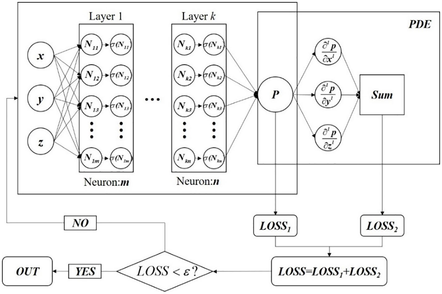
Figure 2 General structure of PINN.

As shown in Figure 2, PINN consists of two parts: the deep neural network prediction part and the partial differential equation constraint part. Using the location $(x,y,z)$ as input, the predicted value $P$ in the region $\Omega$ is predicted after passing through the fully connected layer. The mean square error is calculated as the loss function 1, denoted as $LOS{S}_1$ in Figure 2. The predicted value is put into the pre-set partial differential equation and its loss function $LOS{S}_2$ is calculated. Finally, two kinds of loss functions are combined to train the deep neural network as constraints.

An optimizer is an algorithm used to optimize the model parameters in deep learning, which updates the model parameters according to the gradient information of the loss function, so that the model can gradually approximate the optimal results. The optimizers commonly used in neural networks are stochastic gradient descent (SGD), Adam, AdaGrad and RMSProp. Two optimizers, SGD and Adam, are used to train the PINN in this paper. SGD is one of the most basic optimizers in neural networks. Adam is an optimizer that combines momentum method and adaptive learning rate adjustment, which is a commonly used optimizer in neural networks.

3 UAFP-PINN

This section introduces the underwater acoustic field prediction model based on physics-informed neural network(UAFP-PINN), builds a fully connected deep neural network with six hidden layers, and uses Helmholtz equation to construct the loss function in the neural network and add it to the training of the neural network. This section introduces the specific content of UAFP-PINN model from three parts: model structure, loss function based on Helmholtz equation and model activation function.

3.1 Frame of prediction

The neural network takes the position coordinate of sound pressure $P$ as the input and the corresponding sound pressure value as the output for training. The network consists of one input layer, six hidden layers and one output layer. In order to verify the difference between two-dimensional and three-dimensional model, two-dimensional and three-dimensional physics-informed neural network is established respectively, and the models are trained using $(x,z,p)$ and $(x,y,z,p)$ as inputs respectively.

The input layer of the neural network is the coordinate information of sound pressure, the output layer is the predicted sound pressure, and there are six hidden layers in this neural network. The number of neurons in the hidden layer was (8, 16, 32, 64, 128, 256) and each neuron is connected by full connection. The $i$ neuron in layer $l-1$ and the $j$ neuron in layer $l$ are connected by weighting parameters $w_{ji}^l$. Each neuron trains the model through input weighting parameters $w_{ji}^l$ and bias terms $b^l$ in layer $l-1$. Figure 3 shows the computational relationship between the two related neurons. In the feedforward model, Formula 5 shows the output of the $k$ neuron in the next layer $l$ (Bishop and Nasrabadi, 2006). $\sigma$ is the activation function, which is covered in the third part of this section.

FIGURE 3

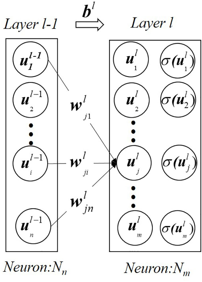
Figure 3 Computational relationship between adjacent neurons.

$\begin{array}{ll}{u}_k^l=\sigma \left({\sum }_{j=1}^{N_{l-1}}{w}_{kj}^l{u}_j^{l-1}+b_k^l\right)& (5)\end{array}$

3.2 Loss function

The key of physics-informed neural network is to train the neural network with physical partial differential equation which describes the state of object. The traditional neural network usually use the mean square error of predicted and simulated values to evaluate the training results. In this study, a Helmholtz equation describing underwater sound propagation is added as another loss function. The loss function of the mean square error and the loss function of the physical constraint are used as constraints to train the model. The loss function of mean square error is denoted as $LOS{S}_1$ and the loss function of physical constraint is denoted as $LOS{S}_2$ (Borrel-Jensen et al., 2021).

The reference formula of loss function LOSS₁ is the formula for calculating mean square error, and the specific content is shown in Formula 6:

$\begin{array}{ll}MSE=\frac{1}{n}{\sum }_{i=1}^n{\left|P_i-T_i\right|}^2& (6)\end{array}$

In the above formula, MSE represents the mean square error, n is the total number of samples, P is the predicted value, and T is the true value. Formula 6 is one of the important indicators to measure the accuracy and precision of the prediction model.

For the prediction model in this paper, the sound pressure value predicted by the neural network is denoted as ${\mathit{p}}^{pre}$, the corresponding simulated sound pressure value is denoted as ${\mathit{p}}^{tra}$, and the number of samples is denoted as N, then the mean square error loss function LOSS₁ of the neural network is shown as Formula 7:

$\begin{array}{ll}LOS{S}_1=\frac{1}{N}{\sum }_{i=1}^N{(p_i^{pre}-p_i^{tra})}^2& (7)\end{array}$

The mean square error loss function LOSS₁ represents the degree of similarity between the predicted value and the simulated value. Traditional neural networks use this loss function to continuously approximate the predicted value to the simulated value. In essence, the model trained by means of the mean square error loss function represents the characteristics of the data dimension.

The sound pressure value ${\mathit{p}}^{pre}$ predicted by the neural network is a function of spatial coordinates, and the Laplacian operator of the sound pressure p in formula 4 can be expressed as:

$\begin{array}{ll}{\nabla }^{2}p=\frac{{\partial }^{2}p}{\partial x^2}+\frac{{\partial }^{2}p}{\partial y^2}+\frac{{\partial }^{2}p}{\partial z^2}& (8)\end{array}$

According to Formula 4, $k$ is the medium beam and the calculation formula is $k=\frac{\omega }{c}$, $\omega$ is the radiation frequency, $c$ is the medium sound speed. Bringing Formula 8 into Formula 4 gives the Helmholtz equation with the predicted values.

$\begin{array}{ll}L=\frac{{\partial }^2{p}^{pre}}{\partial x^2}+\frac{{\partial }^2{p}^{pre}}{\partial y^2}+\frac{{\partial }^2{p}^{pre}}{\partial z^2}+k^2{p}^{pre}& (9)\end{array}$

Formula 9 describes the Helmholtz equation of the predicted value of the neural network, which is a vector, and defines the square of the 2-norm of this vector as the loss function LOSS₂ of the physical constraint (Song et al., 2022), from which the expression of the loss function of the physical constraint can be obtained as:

$\begin{array}{ll}LOS{S}_2=║\frac{{\partial }^2{\mathit{p}}^{pre}}{\partial {\mathit{x}}^2}+\frac{{\partial }^2{\mathit{p}}^{pre}}{\partial y^2}+\frac{{\partial }^2{\mathit{p}}^{pre}}{\partial z^2}+k^2{p}^{pre}{║}_2^2& (10)\end{array}$

The physical constraint loss function LOSS2 represents the physical characteristics of the predicted value and brings the predicted value into the Helmholtz equation describing the underwater sound field. The model trained with the loss function 2 represents the characteristics of the physical dimension.

In order to make the trained neural network have both data characteristics and physical characteristics, the mean square error loss function LOSS₁ and physical constraint loss function LOSS₂ will be combined in this paper. In order to make the model better fitting effect and have strong physical interpretability, the two loss functions will be summed with the same weight. As a whole, the LOSS function LOSS trains the model. The model trained by the LOSS function has clear physical interpretability. The calculation formula of the loss function is as follows:

$\begin{array}{ll}LOSS=\frac{1}{N}{\sum }_{i=1}^N{(p_i^{pre}-p_i^{tra})}^2+║\frac{{\partial }^2{\mathit{p}}^{pre}}{\partial x^2}+\frac{{\partial }^2{\mathit{p}}^{pre}}{\partial y^2}+\frac{{\partial }^2{\mathit{p}}^{pre}}{\partial z^2}+k^2{\mathit{p}}^{pre}{║}_2^2& (11)\end{array}$

3.3 Activation function

As an important parameter in deep neural network training, the activation function ($\sigma$) has great influence on the training efficiency and prediction accuracy of the neural network. The activation functions are mainly used to introduce nonlinear properties that enables neural networks to learn and represent complex nonlinear relationships. The activation function is typically applied to each neuron in a neural network, converts the input signal to nonlinear and passes the transformed result to the next layer. In the training of neural network, common activation functions mainly include tangent activation function ($Tanh(x)$), sine activation function ($\text{sin}(x)$), Relu function ($\text{Relu}(x)$), and arctangent activation function ($Atan(x)$). The images of these four activation functions are shown in Figure 4.

FIGURE 4

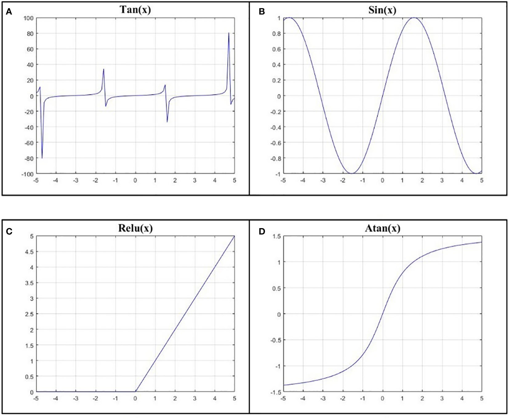
Figure 4 (A) is the tangent activation function, (B) is the sine activation function, (C) is the Relu activation function, and (D) is the arctangent activation function.

The tangent function is more commonly used in cases where the neuronal output has negative values, such as symmetric centralized data. Using tangential activation functions can help neural network introduce nonlinear transformations so that neural network can learn and represent more complex patterns and relationships. The tangent activation function outputs a negative value when the input is negative and a positive value when the input is positive. This makes the tangent activation function more suitable for processing data with positive and negative symmetries.

The sine function is a nonlinear activation function that maps the input values to an output range between -1 and 1. Sine activation functions have nonlinear properties, which can help neural network model learn and represent nonlinear patterns and relationships.

The Relu function is one of the widely used activation functions in deep learning, especially in the hidden layer. Its main advantages are computational efficiency and avoiding gradient saturation problems. Relu function passes positive values and truncate negative values to zero, which makes Relu sparsely active, that is, only some neurons are activated while others are zero. Sparse activation can provide higher model representation and help to reduce the computational load and complexity of the model.

The arctangent function can help mitigate gradient vanishing or gradient explosion problems in some cases because it has a gentler gradient as the input approaches the boundary, and these problems can affect the model’s learning ability and convergence.

In this study, the tangent function, the sine function, the Relu function and the arctangent function (Al-Safwan et al., 2021; Song et al., 2022) are used to predict the model. Different activation functions are selected to observe the decline of the model’s loss function, and the effect of different activation functions is evaluated according to the model prediction effect. Finally, we select the activation function that best fits PINN model.

4 Experiment

4.1 Data

In order to verify the feasibility of the physics-informed neural network, an ocean environment model is established using COMSOL software. A point sound source is placed at the edge of the ocean environment to simulate the excitation conditions of the underwater acoustic field, and the effectiveness of the physics-information neural network is verified according to the acoustic field data.

The test area is 30 meters long, 10 meters wide and 10 meters high, and the test point sound source is located at coordinates (0,5,5). The upper boundary of the area is the air-sea interface, which can be approximated as an absolute soft boundary, and the sound pressure values on the boundary are satisfied the condition $p(x,y,z)=0$; the lower boundary of the area is a hard submarine interface, which can be approximated as an absolute hard boundary, and the sound pressure values on the boundary are satisfied the formula $\frac{\partial p}{\partial z}=0$. The surrounding boundary is a perfectly matched layer (Chen et al., 2013). Due to the small scale of the area, the density of seawater in the area can be approximately constant, the average density of seawater is 1025 $kg/m^3$, and the sound velocity in the seawater medium is 1500 $m/s$. The structure of the area model is shown in Figure 5.

FIGURE 5

Figure 5 Area model structure.

In order to avoid the influence of reverberation on the acoustic field, the point sound source with a frequency of 100 Hz is selected in this paper, the sound wave is a sine wave, and the amplitude is selected as one. Figure 6 shows the spatial acoustic field distribution at 0.1s drawn by COMSOL according to the above conditions, and Figure 7 shows the sound pressure distribution at XZ-plane when coordinate $y$ is five meters.

FIGURE 6

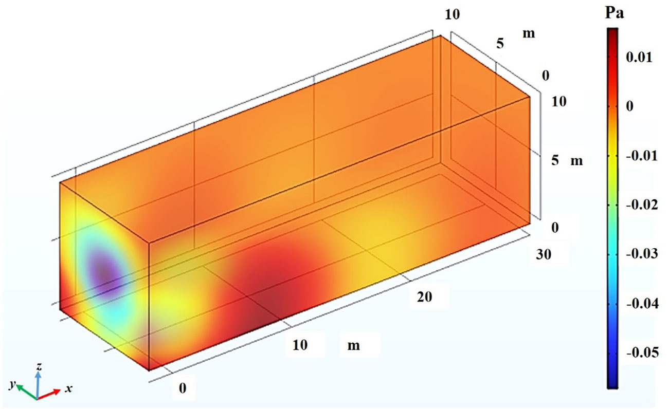
Figure 6 Sound pressure distribution at t= 0.1s.

FIGURE 7

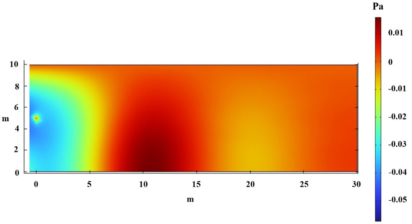
Figure 7 Sound pressure distribution in the XZ-plane at y=5 m.

In this paper, the sound pressure data in 2-dimensional plane and 3-dimensional space are predicted respectively. In this study, prediction data and test data are separated. A total of 28,100 sets of simulated values are collected in the 2-dimensional plane data training set and 112,400 sets of simulated values are collected in the test set. A set of 2-dimensional plane training data is collected every 0.1 m. A total of 352,500 sets of simulated values are collected in the 3-dimensional training set and 982,150 sets of simulated values are collected in the test set. A set of 3-dimensional training data is collected every 0.2 m.

4.2 Introduction to experimental environment

The experimental environment will affect the predicted rate, so this section describes the hardware configuration for the experiment. The GPU is NVIDIA GeForce GT370, the CPU is Intel i7-9700, the operating system is Windows10, and the memory is 64 GB. This paper establishes a prediction model based on Python language, and uses Pytorch framework to establish a neural network. The compiler uses Pycharm2018.

4.3 Hyper parameter setting

In the experiment, the adaptive moment estimation (Adam) optimizer and stochastic gradient Descent (SGD) are used to analyze the influence of the optimizer on the prediction accuracy of the model. For this optimization process, the first-order momentum factor, second-order momentum factor and Fuzz factor in Adam are configured as 0.9, 0.999 and 0.0000001, respectively. The initial learning rate is set to 0.001, the weight attenuation factor is set to 0.0005, and 1/10 of the total training data is used for a batch. Before the actual test, a small batch of test data was used for training, and it is found that the model could converge within 100 times. Therefore, the number of iterations of the 2-dimensional model is set to 500 epochs and the number of iterations of the 3-dimensional model was set to 250 epochs. Finally, in order to ensure that the weight of data-driven and physical constraints is the same, the two loss functions are summed with the same proportional coefficient 1 and combined into an overall loss function to train the model. For the specific loss function, see Formula 11.

4.4 Results and analysis

In order to verify the effectiveness of the underwater acoustic field prediction model, 2D underwater acoustic prediction model based on physics-informed neural network (2D UAFP-PINN) and 3D underwater acoustic prediction model based on physics-information neural network (3D UAFP-PINN) are established by using 2D and 3D acoustic field data. The two models are used to predict the acoustic field data of the test location, adjust different optimizers and activation functions to analyze the optimal model parameters, and finally evaluate the model by analyzing the statistical characteristics between the predicted values and the simulated values.

4.4.1 2D UAFP-PINN

In this section, a 2D underwater acoustic prediction model based on physics-informed neural network (2D UAFP-PINN) is established, and the effects of different activation functions and optimizers on the prediction accuracy of the model are analyzed. Model parameters are as follows: there are 28100 sets of training data and 112,400 sets of test data;The training iteration epochs are 500 times, the data of each training is 1/10 of the total training data. It selects different activation functions and optimizers to train the model and gets the curve of loss function with training times. Figure 8 shows the change curves of the different loss functions using the two optimizers. Since the loss function reached the optimal trend after about 100 training times, only the results of the first 100 training times are shown in the figure to make it clearer.

FIGURE 8

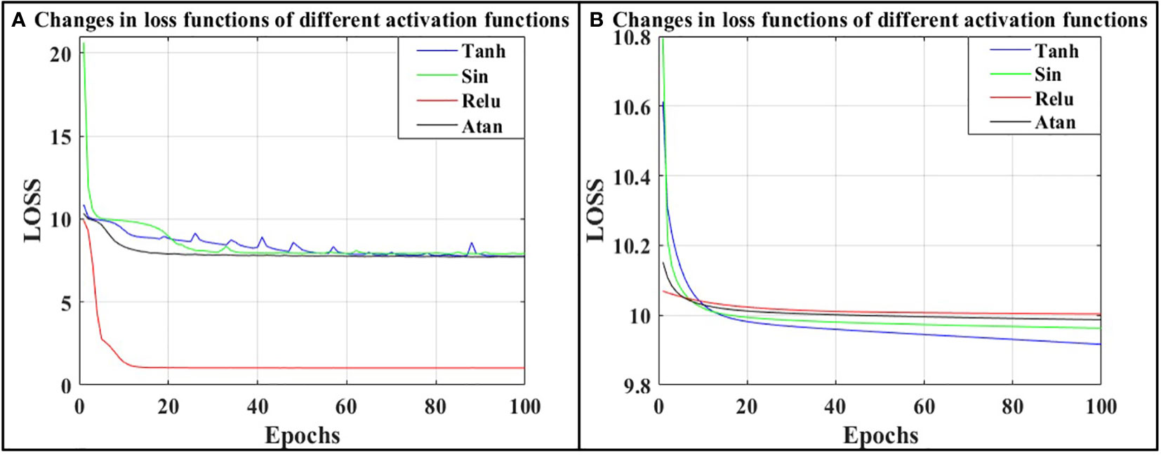
Figure 8 (A) shows the different loss function changes under the Adam optimizer, (B) shows the different loss function changes under the SGD optimizer.

As can be seen from Figure 8, when the Relu activation function is combined with the Adam optimizer, the loss function drops to the lowest values, reaching 1.09, and the minimum trend is reached when the training times are about 13 times. The model convergence speed is faster than other activation functions. Therefore, using the Adam optimizer, the loss function decreases faster than the SGD optimizer, indicating that the Adam optimizer is more suitable for the training of 2D UAFP-PINN model. In summary, it can be seen that using the Adam optimizer and Relu activation function is the best choice for the 2D UAFP-PINN model.

In order to verify the prediction effect of this model, 112,400 sets of data simulated by COMSOL are selected as simulation values to evaluate this model. In this paper, the validity of the forecast results is analyzed from four perspectives: R-squared (R²), mean square error (MSE), mean absolute error (MAE) and absolute error distribution. R-squared is a common regression model evaluation metric used to measure the model’s ability to explain the target variable. The value range of R-squared is between zero and one, when it is closer to one indicates that the model has a better ability to explain the target variable, and when it is closer to zero indicates that the model has a worse ability to explain the target variable. The expression of R-squared is as follows:

$\begin{array}{ll}{R}^2=1-\frac{SSE}{SST}=1-\frac{\sum {(y_i-\widehat{y_i})}^2}{\sum {(y_i-\overline{y})}^2} & (12)\end{array}$

Where $y_i$ are the simulated values of the test set, $\widehat{y_i}$ are the predicted values by PINN, $\overline{y}$ are the mean of the simulated values. $SSE$ represents the sum of squares of residuals, which is the sum of squares of the difference between the predicted values and the simulated values. $SST$ represents the total sum of squares, which is the sum of squares of the difference between the predicted values and the mean of the simulated values.

The formula for calculating the mean square error can be referred to formula 6 in Section 3.2 of the article. The formula for calculating the mean absolute error is as follows:

$\begin{array}{ll}MAE=\frac{1}{n}{\sum }_{i=1}^n\left|P_i-T_i\right|& (13)\end{array}$

In the above formula, MAE represents the mean absolute error, n is the total number of samples, P is the predicted value, and T is the true value.

Table 1 shows the results of R-squared, mean square error and absolute mean values error of predicted values and simulated values of different activation functions under the Adam optimizer, and Figure 9 shows the absolute error distribution of predicted and simulated values of different activation functions. Table 1 and Figure 9 show the statistical characteristics between the predicted values and the simulated values.

TABLE 1

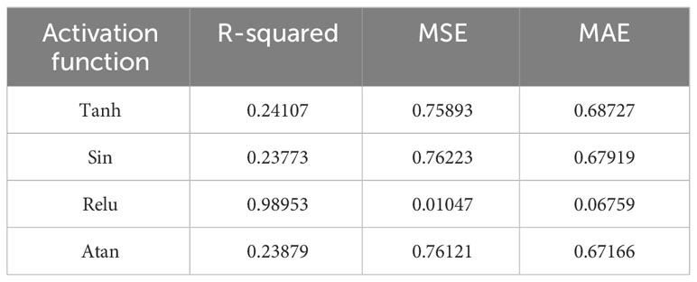
Table 1 Statistical results of different activation functions.

FIGURE 9

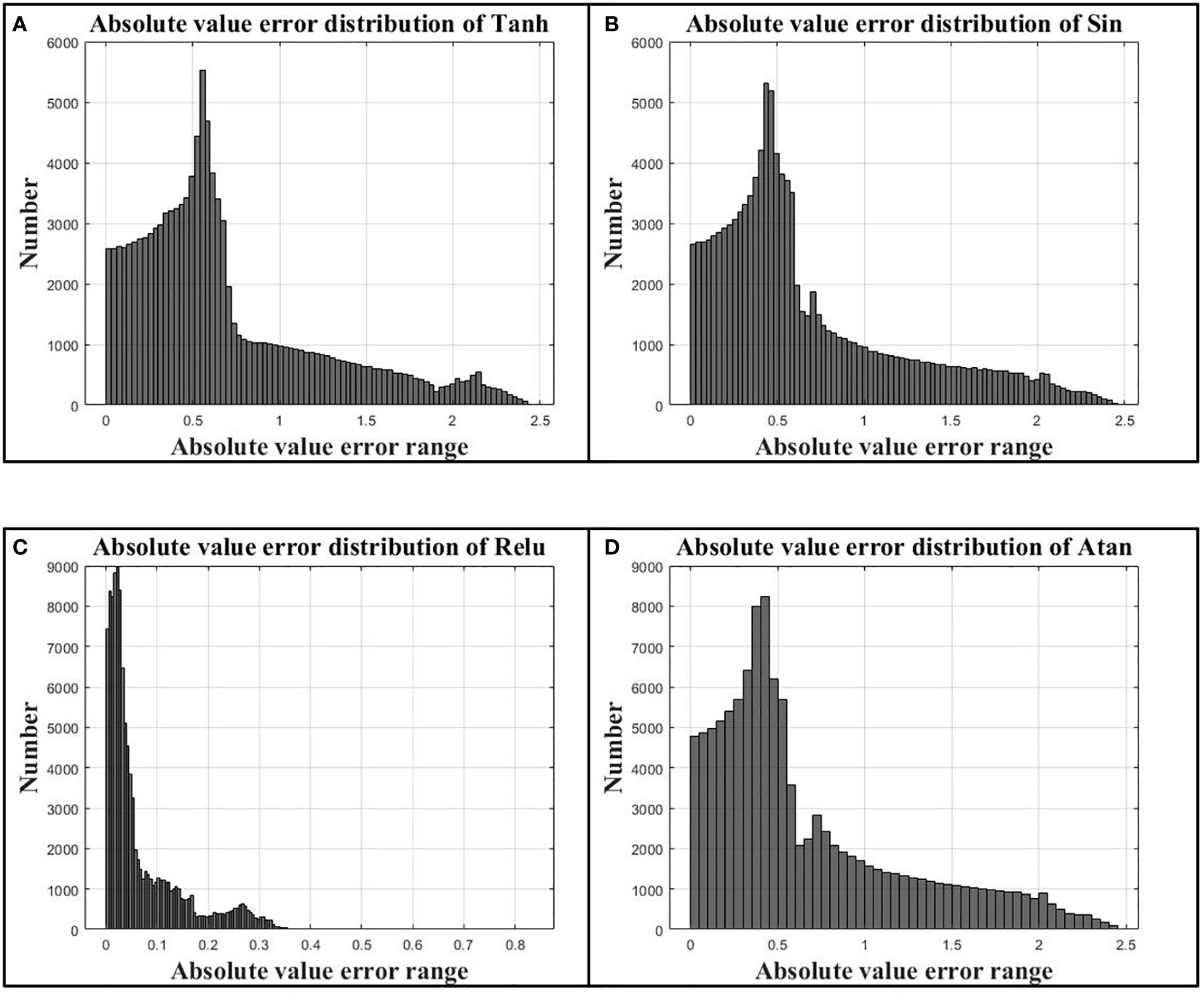
Figure 9 (A) is the absolute error distribution using Tanh activation function, (B) is the absolute error distribution using Sin activation function, (C) is the absolute error distribution using Relu activation function, and (D) is the absolute error distribution using Atan activation function.

The R-squared values represents the correlation between the predicted values and the simulated values, and the larger the value, the stronger the correlation between the predicted values and the simulated values. It can be seen from Table 1 that the model using Relu activation function for prediction has the strongest correlation with the simulated values, that the R-squared value is 0.98953.The mean square error between the predicted values and the simulated values is only 0.01047 Pa when the model uses Relu activation function, and the mean square error of other activation functions are all around 0.75.The mean absolute error between the predicted values and the simulated values is only 0.06759 Pa when the model uses Relu activation function, and other activation functions’ mean absolute error are all around 0.67 Pa. The data predicted by the Relu activation function is very close to the simulated values. Figure 9 shows the distribution of absolute error between the predicted and simulated values of several activation functions. It can be analyzed from the figure that the absolute error of the data predicted by the Relu activation function is distributed within 0.05 Pa, and the data with an absolute error higher than 0.3 Pa is basically not distributed, while the error distribution of the other three activation functions are basically similar, and most of them are concentrated within 1.5 Pa. It can be analyzed that the prediction accuracy is much lower than that of the Relu activation function. Therefore, the best activation function and optimizer for this model are Relu and Adam.

4.4.2 3D UAFP-PINN

In this section, a 3D underwater acoustic prediction model based on physics-informed neural network (3D UAFP-PINN) is established, and the effects of different activation functions and optimizers on the prediction accuracy of the model are analyzed. Model parameters are as follows: there are 352500 pieces of training data and 982150 sets of test data; The training iteration epochs are 250 times, the data of each training is 1/10 of the total training data. It selects different activation functions and optimizers to train the model and gets the curve of loss function with training times. Figure 10 shows the variation curves of the different loss functions using the two optimizers. The optimal trend reached by the loss function after about 20 training sessions. To make it clearer, Adam only shows the results of the first 100 training sessions in the figure, while SGD only shows the results of the first 20 training sessions.

FIGURE 10

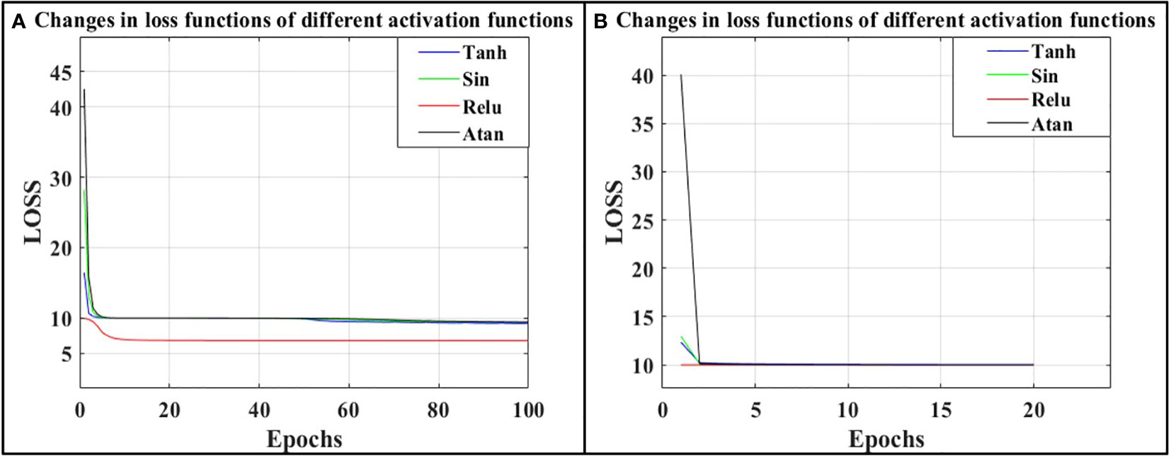
Figure 10 (A) shows the different loss function changes under the Adam optimizer, (B) shows the different loss function changes under the SGD optimizer.

It can be seen from Figure 10 that when Relu activation function and Adam optimizer are used, the loss function decreases to the lowest degree, reaching 6.94, and reaches the lowest trend when the training times are about 10 times. The model convergent speed is faster than other activation functions. The loss function has the best decreasing effect when the optimizer chooses Adam. It can be concluded that the loss function reduction effect using the Adam optimizer is slightly better than that of the SGD optimizer. In summary, it can be seen that using the Adam optimizer and the Relu activation function is the best choice for the PINN framework. However, compared with the two-dimensional training model, with the increase of data dimension, the training complexity greatly increases, and the gap between the optimization effect of the optimizer and the activation function on the network is also significantly reduced, which indicates that with the increase of data dimension, it is necessary to appropriately increase the network complexity to represent the features of higher-dimensional data. Simply changing the activation function and the optimizer does not make the model convergence better.

In order to verify the prediction effect of the model, 982,152 pieces of data were selected to evaluate the model. Table 2 shows the results of R-squared, mean square error and absolute values error of the predicted values and the simulated values using different activation functions under the Adam optimizer. Figure 11 shows the absolute error distribution between the predicted values and the simulated values of different activation functions, which is used to visually display the error distribution of the predicted values.

TABLE 2

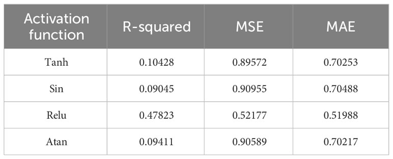
Table 2 Statistical results of different activation functions.

FIGURE 11

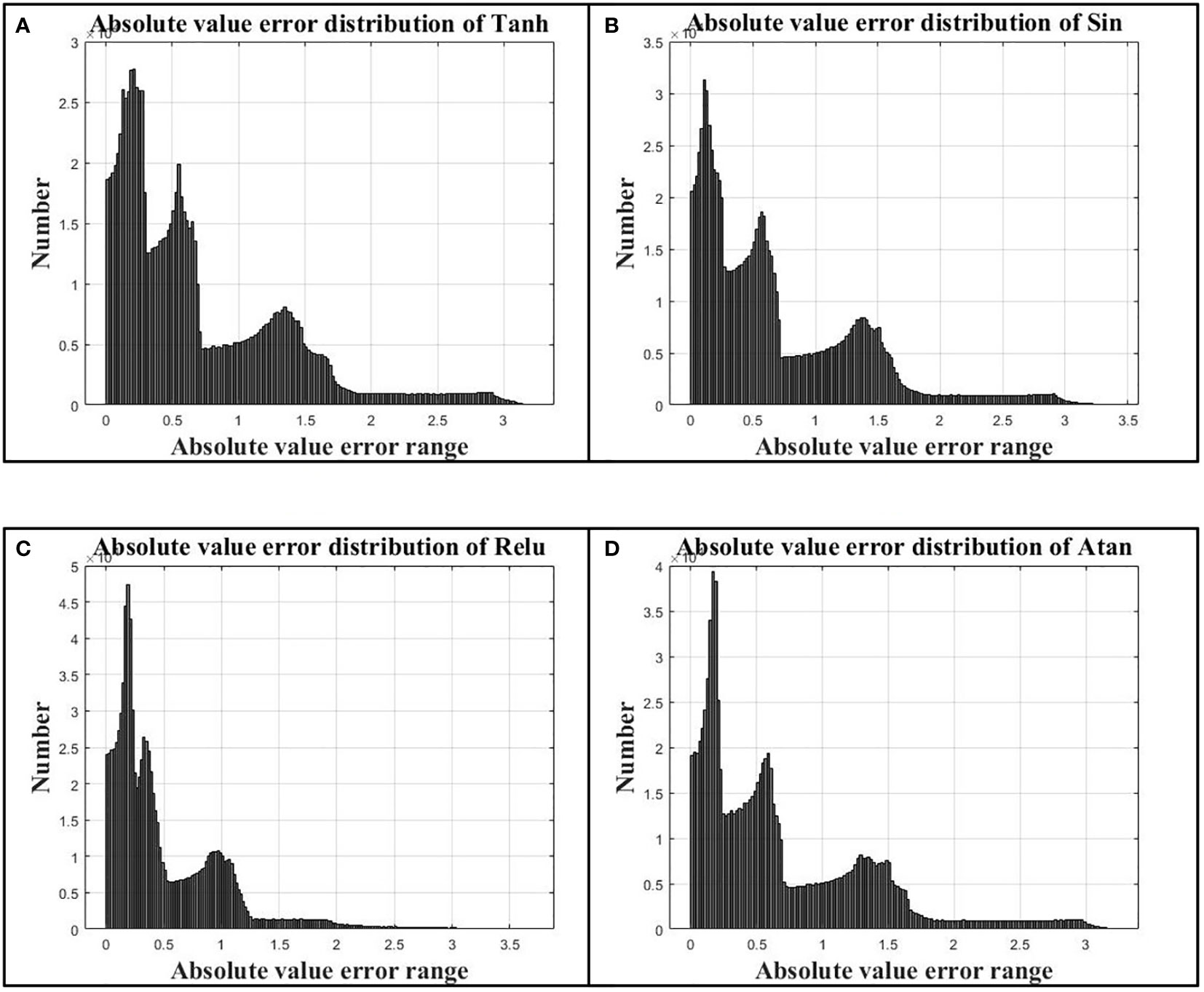
Figure 11 (A) is the absolute error distribution using Tanh activation function, (B) is the absolute error distribution using Sin activation function, (C) is the absolute error distribution using Relu activation function, and (D) is the absolute error distribution using Atan activation function.

As can be seen from Table 2, the largest R-squared value is the result predicted by Relu activation function, which reaches 0.47823, and the predicted values have a relatively high correlation with the simulated values. The correlations of the other three functions are very low. From the mean square error and the mean absolute error, it can be seen that the prediction effect of Relu activation function is much better than that of other activation functions. From the absolute error distribution in Figure 11, the absolute error range of the four activation functions is basically the same, but the absolute error of Relu activation function is mostly concentrated within 0.5 Pa, and the absolute error distribution is the largest around 0.25 Pa, and there is a small peak around 1.0 Pa. However, compared with the prediction results of other activation functions, the prediction effect of Relu activation function is obviously better than that of the other three activation functions.

Comparing the 2D UAFP-PINN and 3D UAFP-PINN training and forecasting results, under the condition of Adam optimizer and Relu activation function, the 2D UAFP-PINN model is much better than the 3D UAFP-PINN model, and the error difference between the two models can reach tens of times. The reason for the big difference between the two models is that the complexity of the acoustic field will also increase with the increase of the dimension of the forecast data. Therefore, if the number of hidden layers and neurons of the 3D model remains the same as that of the 2D model, the fitting effect of the 3D model will have the problem of underfitting. If the dimension of the prediction model is increased, the number of hidden layers and neurons of the model should be increased to match the corresponding complexity and prevent the problem of underfitting.

5 Conclusion

Compared with the numerical method to solve the underwater acoustic field, PINN has the advantage that it can handle the acoustic field of different media and irregular shape models. PINN does not use a regular network to predict the acoustic field. It can be predicted at any point in the input region if the position is known, and there is no limit to the irregular shape of the model. For the three-dimensional acoustic field, the calculation cost of the numerical method will increase sharply due to the addition of one dimension of the data, and PINN can quickly forecast the high-dimensional acoustic field space.

In addition to PINN, there are machine learning-based methods to predict acoustic fields. Onasami et al. (2021) used deep neural networks and long and short time memory networks to model underwater acoustic channels, and established a data-driven underwater acoustic channel model. The acoustic field prediction model based on machine learning is mainly a data-driven method, which needs a lot of training data to support, and has certain timeliness. The underwater acoustic field is time-varying, and it is often difficult to predict the time-varying underwater acoustic field when the model is trained using only historical data. The advantage of PINN is that new constraint variables can be added via partial differential equations, and it has good environmental adaptability. According to the experimental data, the convergence rate of the model loss function is fast.

The experimental results show that PINN using Relu activation function and Adam optimizer can effectively predict the underwater acoustic field. The model is constrained by the Helmholtz equation describing the underwater acoustic field and combined with the excellent model approximation characteristics of the neural network. It can realize the acoustic field prediction in the case of small samples. The Helmholtz equation, which describes the underwater acoustic field, gives the parameters that affect the acoustic field, such as medium density, medium sound velocity, sound source position, vibration frequency, etc. These parameters cannot be given directly in the loss function as constraints to be trained. For the underwater acoustic field of large-scale medium, the sound velocity and the density of medium change with space, so it is difficult for the network to predict the underwater acoustic field of large-scale medium. The main limitation of the underwater acoustic field prediction model proposed in this paper is that the scale of trained model is small. If the source frequency, medium density, and medium sound velocity change, the new network model needs to be retrained separately for these changing conditions. To solve this problem, the source position, medium density, sound velocity and different boundary conditions can be used as new inputs to train the network model together with the coordinate information. Song et al. (2022) and Alkhalifah et al. (2020) used the similar method to generate wave field solutions of multiple seismic sources with one network, and solved the problem of seismic field adaptation of different seismic sources. In addition, time can also be used as input to add time constraint term to Helmholtz equation, and it can establish a kind of physics-informed neural network for spatial-time cooperative prediction. Finally, the combination of transfer learning and PINN is a research direction to solve the problem of underwater sound field model prediction in different scenes.

Using PINN to predict underwater acoustic field, it is necessary to adjust the structure and training amount of prediction network according to the complexity of acoustic field. By comparing the prediction results of 2D UAFP-PINN and 3D UAFP-PINN models in this paper, the following conclusions can be drawn: with the increase of model dimensions, the complexity of model prediction will increase accordingly, and simply changing the activation function and optimizer cannot effectively improve the prediction accuracy of the model. For acoustic fields with more complex dimensions, it is necessary to increase the complexity of the model with more neurons and hidden layers to adapt to more complex physical environments, so as to achieve better prediction results.

In this paper, it establishes physics-informed neural network to forecast underwater acoustic field. By analyzing several activation functions and the accuracy of the results predicted by the optimizer, it is found that the Relu activation function and the Adam optimizer can accurately predict the sound pressure value of the two-dimensional acoustic field. For three-dimensional space, the accuracy of PINN prediction is lower than the two-dimensional acoustic field prediction model, because the complexity of the problem increases with the increase of the dimension of acoustic field. Therefore, it is also necessary to adjust the number of hidden layers and the number of neurons in the network structure. The two-dimensional and three-dimensional neural network structure in this paper is the same as that of neurons, and subsequent work can be verified in this direction. Compared with the numerical method, this method can adapt to different media environments, has certain physical characteristics, and the prediction accuracy can be improved by adjusting the network structure and parameters, so it is an effective method for underwater acoustic field prediction.

Data availability statement

The raw data supporting the conclusions of this article will be made available by the authors, without undue reservation.

Author contributions

LD: Funding acquisition, Investigation, Supervision, Validation, Writing – original draft, Writing – review & editing. ZW: Conceptualization, Data curation, Formal Analysis, Methodology, Resources, Visualization, Writing – original draft, Writing – review & editing. ZL: Funding acquisition, Investigation, Supervision, Validation, Writing – original draft, Writing – review & editing. LW: Investigation, Supervision, Validation, Writing – original draft, Writing – review & editing. DH: Investigation, Supervision, Writing – original draft, Writing – review & editing.

Funding

The author(s) declare financial support was received for the research, authorship, and/or publication of this article. This work was supported by several funding sources, including the Shandong Province “Double-Hundred” TalentPlan (WST2020002), the National Key R&D programs (2022YFC2808003;2023YFE0201900) and the Qingdao Natural Science Foundation funded project "Research on Underwater Acoustic Communication Technology of Underwater Unmanned Platform Under Acoustic Compatibility" (23-2-1-100-zyyd-ch).

Acknowledgments

The authors would like to thank the teachers and students of the Underwater Acoustic Laboratory of Shandong University of Science and Technology for their support of this paper.

Conflict of interest

The authors declare that the research was conducted in the absence of any commercial or financial relationships that could be construed as a potential conflict of interest.

Publisher’s note

All claims expressed in this article are solely those of the authors and do not necessarily represent those of their affiliated organizations, or those of the publisher, the editors and the reviewers. Any product that may be evaluated in this article, or claim that may be made by its manufacturer, is not guaranteed or endorsed by the publisher.

References

Ahmed A. B. R., Younis M., De Leon M. ,. H. (2021). “Machine learning based sound speed prediction for underwater networking applications,” in 2021 17th International Conference on Distributed Computing in Sensor Systems (DCOSS). (Pafos, Cyprus: IEEE), 436–442. doi: 10.1109/DCOSS52077.2021.00074

CrossRef Full Text | Google Scholar

Alkhalifah T., Song C., Waheed U. (2020). “Machine learned Green’s functions that approximately satisfy the wave equation,” in the SEG International Exposition and Annual Meeting. (SEG). doi: 10.1190/segam2020-3421468.1

CrossRef Full Text | Google Scholar

Al-Safwan A., Song C., Waheed U. (2021). “Is it time to swish? Comparing activation functions in solving the Helmholtz equation using PINNS,” in 82nd EAGE Annual Conference & Exhibition. (European Association of Geoscientists & Engineers), 2021 (1), 1–5. doi: 10.3997/2214-4609.202113254

CrossRef Full Text | Google Scholar

Belibassakis K. A., Athanassoulis G. A., Papathanasiou T. K., Filopoulos S. P., Markolefas S. (2014). Acoustic wave propagation in inhomogeneous,layered waveguides based on modal expansions and hp-FEM. J.Wave Motion. 51 (6), 1021–1043. doi: 10.1016/j.wavemoti.2014.04.002

CrossRef Full Text | Google Scholar

Bishop C. M., Nasrabadi N. M. (2006). Pattern recognition and machine learning (New York: Springer).

Google Scholar

Borrel-Jensen N., Engsig-Karup A. P., Jeong C. H. (2021). Physics-informed neural networks for one-dimensional sound field predictions with parameterized sources and impedance boundaries. J.JASA Express Lett. 1 (12), 122402. doi: 10.1121/10.0009057

CrossRef Full Text | Google Scholar

Chen Z., Cheng D., Feng W., Wu T. (2013). An optimal 9-point finite difference scheme for the Helmholtz equation with Pml. J.International J. Numerical Anal. Modeling. 10 (2), 389–410.

Google Scholar

Du G., Tan J., Song P., Xie C., Wang S. (2023). 3D traveltime calculation of first arrival wave using physics-informed neural network. J.Oil Geophysical Prospecting. 58 (01), 9–20. doi: 10.13810/j.cnki.issn.1000-7210.2023.01.010

CrossRef Full Text | Google Scholar

He J., Li X., Gao W., Liu P., Wang L., Tang R. (2022). “Solving differential equations with neural networks: application to the normal-mode equation of sound field under the condition of ideal shallow water waveguide,” in OCEANS 2022-Chennai (Chennai, India: IEEE), 1–7. doi: 10.1109/OCEANSChennai45887.2022.9775421

CrossRef Full Text | Google Scholar

Jensen F. B., Kuperman W. A., Porter M. B., Schmidt H. (2011). Computational Ocean Acoustics (New York: Springer).

Google Scholar

Karniadakis G. E., Kevrekidis I. G., Lu L., Perdikaris P., Wang S., Yang L. (2021). Physics-informed machine learning. J.Nat Rev. Phys. 3, 422–440. doi: 10.1038/s42254-021-00314-5

CrossRef Full Text | Google Scholar

Kiryanov A. V., Salnikova E. N., Salnikov B. A., Yu N., Slesarev (2015). “Modeling and study of main regularities of the formation of sound fields in randomly inhomogeneous underwater waveguides,” in 2015 Proceedings of Meetings on Acoustics, (AIP). vol. 24. doi: 10.1121/2.0000126

CrossRef Full Text | Google Scholar

Liu B., Huang Y., Chen W., Lei J. (2019). Principles of underwater acoustics (Beijing: Science Press).

Google Scholar

Miller S. E. (1954). Coupled wave theory and waveguide applications. J.Bell System Tech. J. 33 (3), 661–719. doi: 10.1002/j.1538-7305.1954.tb02359.x

CrossRef Full Text | Google Scholar

Onasami O., Adesina D., Qian L. (2021). “Underwater acoustic communication channel modeling using deep learning,” in the 15th International Conference on Underwater Networks & Systems. (New York: Association for Computing Machinery), 1–8. doi: 10.1145/3491315.3491323

CrossRef Full Text | Google Scholar

Pfau D., Spencer J. S., Matthews A. G. D. G., Foulkes W. M. C. (2020). Ab initio solution of the many-electron Schrödinger equation with deep neural networks. J. Phys. Rev. Res. 2 (3), 33429. doi: 10.1103/PhysRevResearch.2.033429

CrossRef Full Text | Google Scholar

Raissi M., Perdikaris P., Karniadakis G. E. (2019). A deep learning framework for solving forward and inverse problems involving nonlinear partial differential equations. J.Journal Nondestructive Evaluation. 378, 686–707. doi: 10.1016/j.jcp.2018.10.045

CrossRef Full Text | Google Scholar

Rotskoff G. M., Mitchell A. R., Vanden-Eijnden E. (2022). “Active importance sampling for variational objectives dominated by rare events: Consequences for optimization and generalization,” in 2nd Mathematical and Scientific Machine Learning Conference. (Proceedings of Machine Learning Research), 145. 757–780.

Google Scholar

Shukla K., Di Leoni P. C., Blackshire J., Sparkman D., Karniadakis G. E. (2020). Physics-Informed neural network for ultrasound nondestructive quantification of surface breaking cracks. J.Journal Nondestructive Evaluation. 39 (3), 1–20. doi: 10.1007/s10921-020-00705-1

CrossRef Full Text | Google Scholar

Song C., Alkhalifah T., Waheed U. B. (2022). A versatile framework to solve the Helmholtz equation using physics-informed neural networks. J.Geophysical J. Int. 228 (3), 1750–1762. doi: 10.1093/gji/ggab434

CrossRef Full Text | Google Scholar

Teng D., Chen H., Zhu N. (2010). “Computer simulation of sound field formed around transducer source used in underwater acoustic communication,” in 2010 3rd International Conference on Advanced Computer Theory and Engineering (ICACTE). (Chengdu, China: IEEE). V1–144-V1-148. doi: 10.1109/ICACTE.2010.5579046

CrossRef Full Text | Google Scholar

Tu H., Wang Y., Lan Q., Liu W., Xiao W., Ma S. (2021). A Chebyshev-Tau spectral meth-od for normal modes of underwater sound propagation with a layered marine environment. J. J. Sound Vibration 492, 115784. doi: 10.1016/j.jsv.2020.115784

CrossRef Full Text | Google Scholar

Tu H., Wang Y., Liu W., Ma X., Xiao W., Lan Q. (2020). A Chebyshev spectral method for normal mode and parabolic equation models in underwater acoustics. J.Mathematical Problems Eng 2020, 7461314. doi: 10.1155/2020/7461314

CrossRef Full Text | Google Scholar

Tu H., Wang Y., Yang C., Wang,. X., Ma S., Xiao W., et al. (2022). A novel algorithm to solve for an underwater line source sound field based on coupled modes and a spectral method. J. J. Comput. Phys. 468, 111478. doi: 10.1016/j.jcp.2022.111478

CrossRef Full Text | Google Scholar

Wu G., Wang F., Cheng S., Zhang C. (2022). Numerical simulation of forwad and inverse problems in internal sound field analysis based on Physics-Informed Neural Network. J.Chinese J. Comput. Phys. 39 (06), 687–698. doi: 10.19596/j.cnki.1001-246x.8520

CrossRef Full Text | Google Scholar

Yang P., Zhang X., Sun H. (2023). An imaging algorithm for high-resolution imaging sonar system. J. Multimedia Tools Appl., 1–17. doi: 10.1007/s11042-023-16757-0

CrossRef Full Text | Google Scholar

Zhang X. (2023). An efficient method for the simulation of multireceiver SAS raw signal. J.Multimed Tools Appl., 1–18. doi: 10.1007/s11042-023-16992-5

CrossRef Full Text | Google Scholar

Zhang Z., Pan Q., Ji W., Huang F. (2022). Prediction of surface settlements induced by shield tunnelling using physical-information neural networks. J.Engineering Mechanics. 39, 13. doi: 10.6052/j.issn.1000-4750.2022.04.0369

CrossRef Full Text | Google Scholar

Zhang X., Wu H., Sun H., Ying W. (2021). Multireceiver SAS imagery based on monostatic conversion. J.IEEE J. Selected Topics Appl. Earth Observations Remote Sensing. 14, 10835–10853. doi: 10.1109/JSTARS.2021.3121405

CrossRef Full Text | Google Scholar

Zhang X., Yang P., Sun H. (2023). An omega-k algorithm for multireceiver synthetic aperture sonar. J. Electron. Letters. 59 (13), e12859. doi: 10.1049/ell2.12859

CrossRef Full Text | Google Scholar

Zhou Y., Luo W. (2021). A finite element model for underwater sound propagation in 2-D environment. J.Journal Mar. Sci. Engineering. 9 (9), 956. doi: 10.3390/jmse9090956

CrossRef Full Text | Google Scholar

Zhu W., Xu K., Darve E., Beroza G. C. (2021). A general approach to seismic inversion with automatic differentiation. J.Computers Geosciences. 151, 104751. doi: 10.1016/j.cageo.2021.104751

CrossRef Full Text | Google Scholar

Zou J., Liu C., Zhao P. (2023). Research progress of physics-informed neural network in seismic wave modeling. J.Progress Geophysics. 38 (01), 430–448. doi: 10.6038/pg2023GG0142

CrossRef Full Text | Google Scholar