Abstract
Whitecapping dissipation is a critical term in affecting the accuracy of wave height modeling. However, the whitecapping dissipation coefficient (Cds), as a primary factor influencing whitecapping, is commonly determined through trial and error in various studies. In this study, we present a general method for calibrating the Simulating Waves Nearshore (SWAN) wave model using the whitecapping dissipation term, demonstrated through a detailed study in the South China Sea (SCS). Theoretical analysis reveals that the optimal Cds value shows a one-to-one correspondence with the applied wind field. Expectedly, under high-quality wind field conditions, the optimal Cds values tend to fall within a narrow range, regardless of the model domain or time span. Numerical experiments executed in the SCS further consolidated this inference, encompassing two common wind input schemes (ST6 and YAN) and three distinct whitecapping dissipation schemes (KOMEN, JANSSEN, and WST). Based on the experimental results, we have identified an optimal Cds range for each whitecapping dissipation scheme. Cds values within the optimal range consistently outperformed the default Cds in the SWAN model. Subsequent experiments verified the method’s applicability to the Gulf of Mexico and the Mediterranean Sea. The findings suggest that this research holds substantial promise for practical applications on a global scale.
1 Introduction
In recent decades, the third-generation wave models that can solve the spectral action balance equation without assuming a priori spectral shape (The WAMDI Group, 1988; Booij et al., 1999) have been widely developed and applied worldwide (Cavaleri et al., 2020; Shao et al., 2023). Among the terms in the wave action equation, whitecapping, responsible for energy dissipation in deep water, remains one of the least understood physical aspects (Rogers et al., 2002; Cavaleri et al., 2019). Several whitecapping expressions had been proposed (Hasselmann, 1974; Komen et al., 1984; Janssen, 1992; Banner et al., 2000; Alves and Banner, 2003; Van der Westhuysen et al., 2007). Early whitecapping expressions were adjusted based on closing the energy balance of waves in fully developed conditions, as exemplified in the work of Komen et al. (1984) (hereinafter referred to as the KOMEN expression or KOMEN). Alves and Banner (2003) refined the KOMEN expression based on observations, proposing an expression predominantly reliant on the ratio of azimuthal-integrated spectral saturation to the saturation spectrum. Van der Westhuysen et al. (2007) proposed a novel whitecapping expression based on Alves and Banner (2003) but removed the dependence on mean spectra, increasing its suitability for nearshore applications. The Simulating Waves Nearshore (SWAN) model, one of the prominent representatives of third-generation wave models, provides 6 whitecapping expressions with 19 adjustable parameters (The SWAN team, 2021a).
Whitecapping plays a fundamental role in achieving the correct energy balance and significantly influences the accuracy of wave models (Roland and Ardhuin, 2014; Cavaleri et al., 2019). Therefore, the selection and tuning of the whitecapping scheme are crucial (Sun et al., 2022). The whitecapping dissipation coefficient (Cds) is a key parameter that integrally controls the whitecapping dissipation, which is not dependent on the wave steepness or the wave number (Sun et al., 2022). Among all the parameters in the whitecapping schemes, Cds is usually used as a tuning parameter in the calibration process (Cavaleri et al., 2018; Cavaleri et al., 2020). Extensive research indicates that suitable schemes and optimal parameters may vary by region or forcing wind field (Shao et al., 2023). For instance, in the Bohai Sea, the KOMEN expression effectively represents the wind-wave characteristics with the Cds of 2.2E-5 (Lv et al., 2014). Appendini et al. (2013) and Amarouche et al. (2019) improved the model performance using the expression proposed by Janssen (1992) (hereinafter referred to as the JANSSEN expression or JANSSEN) but with entirely different optimal Cds in the Mediterranean Sea (MS). Appendini et al. (2013) achieved the optimal combination of Cds at 1.5 and δ (the coefficient determining the dependence of whitecapping on the wave number) at 0.7, whereas Amarouche et al. (2019) found the optimal Cds to be 1.0. Off the west coast of Norway, the expression proposed by Van der Westhuysen et al. (2007) provided the best performance with mixed swell-wind sea conditions (Van der Westhuysen et al., 2007; Christakos et al., 2021) found that default settings of the whitecapping dissipation scheme commonly led to overestimation of the peak frequency and underestimation of the energy level of the spectral peak during high wind speed conditions. Consequently, wave parameters such as significant wave height (SWH) and mean wave period may be underestimated (Elkut et al., 2021; Umesh and Behera, 2021). Although calibrating the model using Cds lacks a valid physical basis, as the simulated whitecapping dissipation may not accurately reflect realistic conditions, this approach is widely acknowledged for improving practical wave simulations (Wu et al., 2021; Bujak et al., 2023).
Most wave modeling studies typically involve conducting multiple experiments over a certain range of Cds and determining the optimal Cds based on simulation results (e.g., Akpinar and Ponce de León, 2016; Kutupoğlu et al., 2018; Bingölbali et al., 2019; Sun et al., 2022). Wu et al. (2021) proposed a novel Cds calibration method that requires at least two experiments to determine the optimal Cds. However, this method relies on a fitting formula based on experimental results, inevitably introducing fitting errors. Although both methods can obtain the optimal Cds, they require significant time and computational resources. Therefore, finding a general method to determine the optimal Cds value is necessary. Overall, the accuracy of wave model results, particularly in SWH, is strongly influenced by the forcing wind field and source term parameterization (Cavaleri and Bertotti, 1997; Zhai et al., 2021). The wind field provides positive energy flux to the wave model, while the dissipation term contributes to negative energy flux (Babanin et al., 2010). Thus, there exists a potential relationship between the wind field and Cds. Based on this concept, it is theoretically feasible to calibrate the wave model.
This study aims to propose a general method for determining the optimal Cds to improve the efficiency of wave simulation. The remaining parts of this paper are structured as follows. Section 2 describes the study area and bathymetry data. Section 3 details the primary data and methods, including the basic principle of SWAN, observations, and error metrics. Section 4 presents the theoretical basis of this work. In Section 5, numerical experiments are conducted to explore the characteristics of the optimal Cds. Section 6 discusses the applicability of the conclusions we have obtained to different regions. Finally, Section 7 provides the conclusion.
2 Study area and bathymetry
The study area of this work encompasses the South China Sea (SCS; 104°E–124°E, 0°–25°N), as delineated by the solid black line box in Figure 1. The SCS is a typical semi-enclosed marine region, connected to the Pacific Ocean and the Indian Ocean through narrow straits or channels (Su et al., 2017; Ou et al., 2018). It features intricate topography, characterized by three distinct elements: the continental shelf that connects to the land, the continental slope at the outer edge of the continental shelf, and the central basin. As depicted in Figure 1, this region is marked by significant variations in water depth, with a maximum depth exceeding 5500 meters and an average depth of approximately 1200 meters. The general pattern is one of shallow waters in the north and south and deeper waters in the central area (Zhang et al., 2020). Given its strategic importance in shipping and trade routes, along with its abundant reserves of oil, natural gas, and fisheries, the SCS holds significant economic and geopolitical value (Wang, 2021).
Figure 1

Bathymetry map of the study area. The black solid line frame denotes the SCS.
The bathymetry data used in this study was interpolated from the General Bathymetric Chart of the Oceans (GEBCO1) dataset. The GEBCO is a global terrain model that provides elevation data on a 15-arc-second interval grid with a resolution of almost 0.46 km (Weatherall et al., 2021). Due to its high resolution, GEBCO accurately depicts near-shore and deep-sea terrain, making it widely used in wave simulation (Akpinar et al., 2016; Kutupoğlu et al., 2018; Beyramzade et al., 2019; Sun et al., 2022).
3 Data and methods
3.1 SWAN model description
The third-generation wave model SWAN is developed at the Delft University of Technology (The SWAN team, 2021b). SWAN is well known for its implicit schemes and iteration techniques, which make the model performance more robust and economic, especially in shallow shelf seas. As a third-generation wind-wave model, SWAN computes the rate of change of wave action density () as follows
The first term on the left-hand-side represents the rate of change of with time, and the second and third terms represent the propagation of waves in geographic space. and are the wave propagation velocities in the zonal and meridional directions respectively. The fourth term represents the shifting of the radian frequency () due to variations in depth and mean currents. The fifth term demotes the depth-induced and current-induced refraction in wave propagation direction (). The right side of this equation, is the superposition of all sink and source terms:
These six terms denote, respectively, wave growth by the wind, wave decay due to whitecapping, bottom friction and depth-induced wave breaking, nonlinear transfer of wave energy through three-wave and four-wave interactions. Detailed descriptions of these terms can be found in the SWAN scientific and technical documentation (The SWAN team, 2021b).
In SWAN, the whitecapping expressions are based on a pulse-based model (Hasselmann, 1974), and remodified by the WAMDI Group (1988):
in which and represent the mean frequency and mean wave number respectively, and is the wave number. is a coefficient related to the wave steepness and has been adapted by Günther et al. (1992) from Janssen (1992):
where is the overall wave steepness, and Cds, and are tunable coefficients. is the value of for the Pierson-Moskowitz spectrum (Pierson and Moskowitz, 1964). Cds has two different choices in SWAN, namely KOMEN and JANSSEN. The default value of Cds is 2.36E-5 for KOMEN but 4.5 for JANSSEN.
Van der Westhuysen et al. (2007) divided the dissipation mode into breaking and non-breaking waves, which were active in different parts of the spectrum:
where and are the contribution by breaking and non-breaking waves, respectively. is the azimuthal-integrated spectral saturation, Br is a threshold saturation level. Br and Cds are both tunable parameters and the default settings in SWAN are Br = 1.75E-3 and Cds = 5.0E-5. However, the theory of non-breaking low-frequency waves is not yet mature, so is usually replaced by KOMEN.
The scheme of Van der Westhuysen et al. (2007) is always used in conjunction with the wind input scheme of Yan (1987) (hereinafter referred to as YAN), and the expression is given as
where C1 = 4.0E-2, C2 = 5.52E-3, C3 = 5.2E-5, C4 = −3.02E-4 are constants (The SWAN team, 2021b), and are the friction velocity and phase speed respectively. In SWAN, the whitecapping scheme of Van der Westhuysen et al. (2007) and YAN are usually treated as a stand-alone scheme, hereinafter referred to as WST.
Since the implementation of the “ST6” source term package (Rogers et al., 2012; The SWAN team, 2021b) (hereinafter referred to as ST6), its good performance at different spatial scales and weather conditions has made it widely used (Liu et al., 2019). According to Zieger et al. (2015) and Rogers et al. (2012), the wind input expression of ST6 is given as
where Bn is the spectral saturation. W1 and W2 represent the positive and adverse wind inputs respectively and their magnitudes are dependent on the friction velocity . a0 is the wind scaling coefficient.
3.2 Model setup
In this study, we used the hindcast model SWAN Cycle III version 41.31AB2. The SWAN model is operated in the third generation and non-stationary mode with a spatial resolution of 0.25° × 0.25°. A time step of 30 minutes is adopted, and each time step is iterated up to a maximum of 5 times. The JONSWAP (Joint North Sea Wave Project) spectrum is divided into 72 directions and frequency bins between 0.04 Hz and 1.0 Hz. The JONSWAP spectrum is used for the bottom friction with Cb (the bottom friction coefficient) setting to 0.038 (Hasselmann et al., 1973). The study period spans from 2017 to 2021. To investigate the effect of different whitecapping schemes, we evaluate three schemes: KOMEN, JANSSEN, and WST. For KOMEN and JANSSEN, we employ the ST6 with the wind drag formula developed by Hwang (2011) and the wind scaling coefficient a0 set to 28. For WST, we still use YAN as the wind input scheme. Due to computational resource limitations, we mainly conduct numerical experiments using these two wind input schemes, ST6 and YAN. The detailed settings of all experiments are provided in Table 1.
Table 1
| Model physics | Parameterization scheme | Parameters | Values |
|---|---|---|---|
| Wind input | ST6 | HWANG | – |
| a0 | 28 | ||
| YAN | – | – | |
| Triad wave–wave interactions | LTA | Ur | 0.01 |
| Quadruplet wave interactions | DIA | λ | 0.25 |
| Cnl4 | 3E+7 | ||
| Bottom friction | JONSWAP | Cb | 0.038 |
| Depth-induced wave breaking | CONSTANT | α | 1.0 |
| γ | 0.73 | ||
| Whitecapping | KOMEN | cds2 | – |
| JANSSEN | cds1 | – | |
| WST | cds2 | – |
Parameter settings of SWAN model.
3.3 Atmospheric forcing data and observations
Forcing wind fields significantly affect the accuracy of wave models (Kutupoğlu et al., 2018; Yang et al., 2022). In this study, we utilized 10-m wind speeds (U10) from three high-quality wind products to drive the wave model, namely the fifth-generation European Centre for Medium-Range Weather Forecasts (ECMWF) Reanalysis (ERA53), the Cross-Calibrated Multi-Platform Version 2.0 (CCMP4), and the National Centers for Environmental Prediction (NCEP) Final Reanalysis Data (FNL5).
The latest atmospheric reanalysis data from ECMWF is ERA5, which supersedes ERA-Interim since September 2019 (Jiang et al., 2022). ERA5 offers a finer spatial grid, higher temporal resolution, and more vertical levels compared to ERA-Interim (Hersbach et al., 2020). The dataset used in this study has a horizontal resolution of 0.25° × 0.25° and a temporal resolution of 1 hour. Previous studies have demonstrated the exceptional performance of ERA5 in our study area (Zhang et al., 2020; Feng et al., 2022; Yang et al., 2022; Zhai et al., 2023). Therefore, ERA5 was selected as the primary forcing wind field to drive the model.
CCMP is a Level-3 ocean vector wind analysis product that provides high-quality global wind field data with a six-hour temporal resolution from 1988 to the present and a spatial resolution of 0.25° × 0.25° (Wentz, 2015; Mears et al., 2019; Wu et al., 2022). Experimental validation conducted by Atlas et al. (2011) demonstrated a significant improvement in the accuracy of CCMP data compared to wind field measurements from individual satellite platforms, rendering it well-suited for oceanic and atmospheric research.
FNL is a global reanalysis product with a six-hour temporal resolution spanning from 1999 to the present and a spatial resolution of 1.00° × 1.00° (Appendini et al., 2013; Chen et al., 2020). It employs an advanced data assimilation system and assimilates observation data from various sources. The product is founded upon the Global Data Assimilation System (GDAS) and is prepared operationally every 6 hours using the identical model and assimilation scheme as the NCEP operational Global Forecast System (GFS).
The Satellite with ARgos and ALtiKa (SARAL6) project is a joint mission operated by the Indian Space Agency (ISRO) and the French Space Agency (CNES), designed for ocean observations (Verron et al., 2015). AltiKa, SARAL’s primary payload, is the first spaceborne altimeter operating at the Ka-band frequency (35.75 GHz). The higher frequency leads to a smaller footprint (8 km diameter) and so a better spatial resolution (Verron et al., 2021). Since March 2013, SARAL has been providing along-track data for various physical oceanographic parameters on a global scale, including sea surface wind speed, SWH, and sea surface height (Verron et al., 2015). Recent studies have affirmed SARAL’s high accuracy, data quality, and availability (Sepulveda et al., 2015; Sharma et al., 2022). SARAL offers a range of processed data products at various levels. In this study, we utilized a delayed-mode version, specifically the Nadir altimeter Geophysical Data Record (GDR).We performed interpolation on the wind-forcing data and simulated SWH data through temporal (cubic spline) and spatial (nearest-neighbor) methods to align them with the altimeter data. To ensure the reliability of our validation results, we excluded the altimeter data that was more than 5 kilometers away from the nearest grid points. The variations in the quantity of valid altimeter data under different conditions are detailed in Table 2.
Table 2
| Gribed data | ERA5 | CCMP | FNL | Simulated SWH |
|---|---|---|---|---|
| Amount of valid data | 68,827 | 67,929 | 16,803 | 68,181 |
Amount of valid altimeter data under different conditions.
3.4 Error metrics
To accurately quantify the model performance, we employed two commonly used error metrics, including the index of agreement (d) proposed by Willmott (1982), and Slope. The specific formula for the d index is presented below
where is the observed value, is the mean value of the observed data, is the value of the wind products or model outputs, and n is the sample size. The d index displays the differences between simulated and observed means and variances, which reflect sensitivity to outliers in the observation data and insensitivity to additional and proportional variances between simulated and observed values (Zheng et al., 2023). Moreover, the d index is a standardized metric, with values ranging between 0 and 1, where values closer to 1 indicate higher consistency between two datasets (Willmott, 1982). The Slope provides an indication of the direction of errors and is calculated as the linear regression coefficient in the regression model y = cx. A Slope value greater (or less) than 1 signifies that tends to be larger (or smaller) than . This paper will primarily use the d index to measure the consistency between and , while the Slope will be used as a secondary measure to assess the direction of errors.
4 Theoretical basis
4.1 The wind errors and Cds
With the wind input scheme determined, the forcing wind field, the only input variable, directly determines the magnitude of the input energy. However, errors in the wind field can affect the simulated SWH. Positive errors in the wind field lead to larger simulated SWH, while negative errors lead to smaller simulated SWH (Wu et al., 2020). Taking physical quantities in real environment as reference, positive errors in the forcing wind field require greater dissipation energy than in reality to maintain energy balance, whereas negative errors require less. It can be inferred that Cds, which is the primary factor influencing dissipation energy, may exhibit a compensatory relationship with wind errors. In order to explore this relationship, sensitivity experiments were conducted. Figure 2A illustrates simulations where the wind field was scaled by factors of 0.8, 0.9, 1, 1.1, and 1.2, with a constant Cds value of 0.22E-5. Likewise, in Figure 2B, simulations were performed using the same wind field but varying Cds values. A comparison between Figures 2A, B reveals that, when Cds is held constant, the simulated SWH gradually increases as the wind field increases. Conversely, when the wind field remains constant, the simulated SWH gradually decreases with increasing Cds. Hence, when the wind errors are determined, the corresponding optimal value of Cds can also be determined.
Figure 2
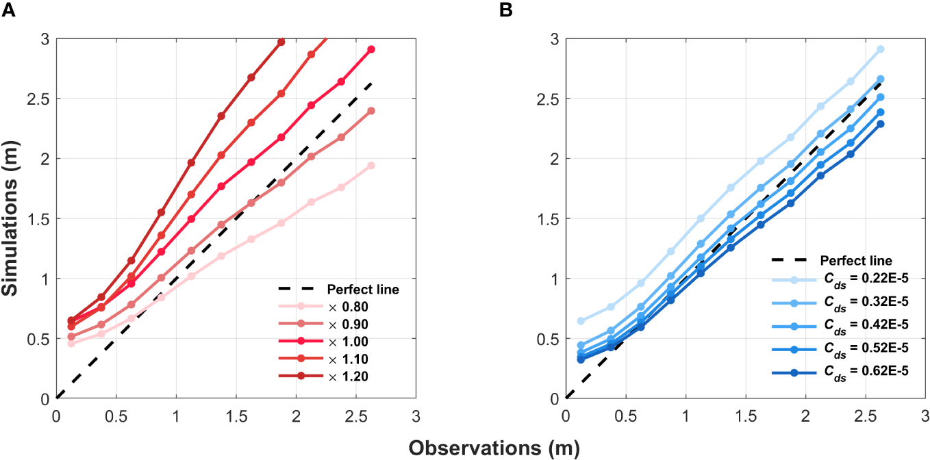
Bin-averaged scatterplots of simulated SWH versus the observations under (A) variable wind fields and (B) variable Cds. In panel (A), ERA5 U10 is scaled at 0.8, 0.9, 1.1, and 1.2 times with a fixed Cds value of 0.22E-5. In panel (B), Cds values are varied at 0.22E-5, 0.32E-5, 0.42E-5, 0.52E-5, and 0.62E-5, while ERA5 U10 remains unchanged.
4.2 The errors in the wind fields
Currently, a wide range of wind field products are available, and with advancements in observation and assimilation techniques, these products consistently demonstrate high quality (Wu et al., 2020; Wu et al., 2022). However, the utilization of diverse assimilation data and methods in different wind field products results in variations in their errors. Figure 3 illustrates the interannual variations in the errors of three wind field products: ERA5, FNL, and CCMP. Analysis of the Slope values reveals a consistent underestimation of actual wind fields by ERA5 over 2017−2021, corroborating findings from previous studies (Shi et al., 2021; Son et al., 2023; Zhai et al., 2023). Furthermore, in 2019 and 2020, all three wind field products exhibited varying degrees of underestimation. When examining the trend of the d index, CCMP consistently displayed the highest quality with a d index of approximately 0.92, while FNL exhibited the poorest quality with a d index of around 0.89. In 2020, there was a fluctuation in the quality of these three wind field products compared to the norm, with a d index of approximately 0.86. Overall, the d index of the three high-quality wind field products ranges from 0.86 to 0.93, and the Slope values are also near 1. This indicates that the errors in each wind field product are relatively stable.
Figure 3
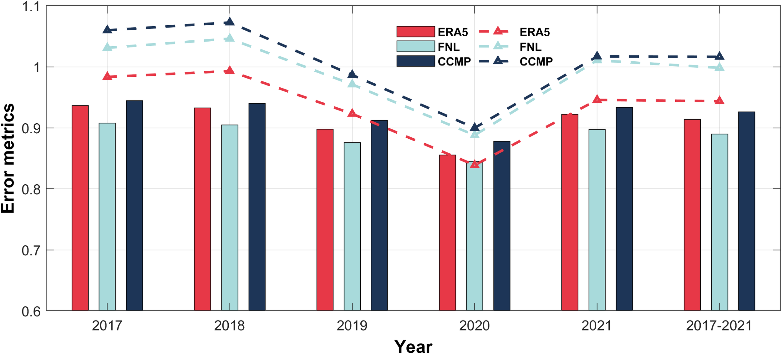
Time series analysis of wind field quality. Red, sky blue, and dark blue are ERA5, FNL and CCMP, respectively. The bars represent the d index, while the dashed line indicates the Slope value. The final point on the X-axis represents the overall error for a five-year period (2017−2021).
Based on the findings in Section 4, it is hypothesized that when using high-quality wind field products, the optimal Cds values will exhibit minimal variability. Therefore, conducting a series of numerical experiments to validate this hypothesis is essential.
5 Numerical experiments
In this section, we will conduct an extensive sensitivity analysis to validate whether the hypothesis proposed in the previous chapter still holds under different seasons, years, and wind field types. If confirmed, we will also determine the specific range of the optimal Cds, which can greatly enhance the accuracy of wave simulation.
According to the conclusions in Section 4, there is a monotonic relationship between Cds and simulated SWH. In other words, as Cds increases, there will inevitably be an optimal simulation effect at a certain value. To determine this optimal simulation accuracy, we search for the maximum value of the d index. Guided by this principle, we initiate our experiments using one-tenth of the default Cds as the starting point and apply a step size of 0.1E-5 or 0.1.
5.1 Sensitivity to different seasons
Firstly, we examine the seasonal characteristics of the optimal Cds values under three distinct whitecapping dissipation schemes using ERA5 as the forcing wind field. Figure 4 illustrates the d index represented by purple bars, the Slope depicted by a black curve, and the maximum value of the d index indicated by a green dashed line, corresponding to the position of the optimal Cds values. The comparison of the d index for each season reveals that the simulation performance in spring is notably inferior to that of other seasons, even when considering the optimal Cds values, as the d index remains below 0.90. Analyzing the simulation results of the three schemes across different seasons shows that WST only achieves a d index above 0.90 in winter, suggesting that the overall simulation performance of KOMEN and JANSSEN surpasses that of WST.
Figure 4
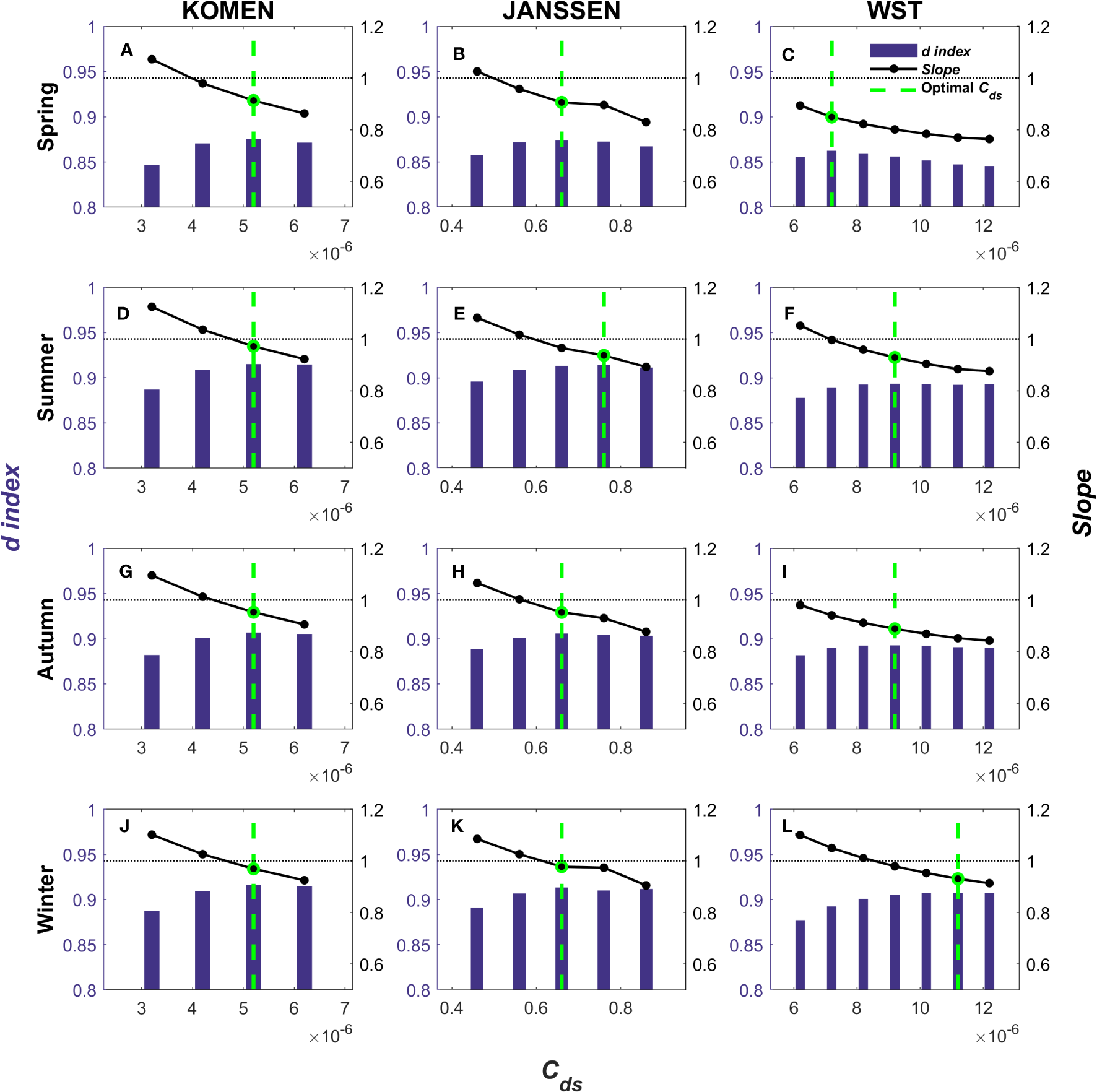
The distributions of d index and Slope for spring (A–C), summer (D–F), autumn (G–I), and winter (J–L). From left to right, (A, D, G, J) are KOMEN; (B, E, H, K) are JANSSEN; (C, F, I, L) are WST. The purple bars show the d index for each experiment, corresponding to the left Y-axis. The solid black line shows the Slope distribution corresponding to the right Y-axis. The green dotted line indicates the experiment corresponding to the maximum value of the d index, that is, the experiment corresponding to the optimal Cds. The black dashed line represents the Slope equal to 1.
Regarding the distribution of the optimal Cds values, KOMEN remains fixed at 0.52E-5, while JANSSEN ranges from [0.66, 0.76], and WST fluctuates within the range of [0.72E-5, 1.12E-5]. It is important to note that reducing the step size of Cds and increasing the number of experiments may yield more accurate values for the optimal Cds, but this is expected to have only a minor impact on the experimental results. Based on the experimental outcomes, it is evident that the three whitecapping dissipation schemes exhibit seasonal fluctuations in the optimal Cds values. However, the magnitude of these fluctuations is minimal.
Based on the observed variations in the Slope, it is evident that an increase in Cds corresponds to a gradual decrease in the Slope, implying a systematic decline in the simulated SWH. This finding reinforces the conclusion established in Section 4. Additionally, it is worth mentioning that at the optimal Cds values, all of the Slope consistently fall below 1, indicating an underestimation of the simulated SWH relative to the observed values. Notably, WST exhibits the most pronounced underestimation among the evaluated schemes.
5.2 Sensitivity to different years
To determine the optimal Cds values for each year, we expanded the range of Cds based on the experiments in Section 5.1. Figure 5 illustrates the interannual characteristics of the optimal Cds values for the three whitecapping dissipation schemes. The optimal Cds range is [0.42E-5, 0.52E-5] for KOMEN, [0.46, 0.86] for JANSSEN, and [0.72E-5, 1.12E-5] for WST. Comparing the seasonal characteristics of the optimal Cds values, JANSSEN exhibits a slightly larger fluctuation, while the other two schemes remain relatively consistent. Overall, we can conclude that the interannual variability of the optimal Cds values is also very small.
Figure 5
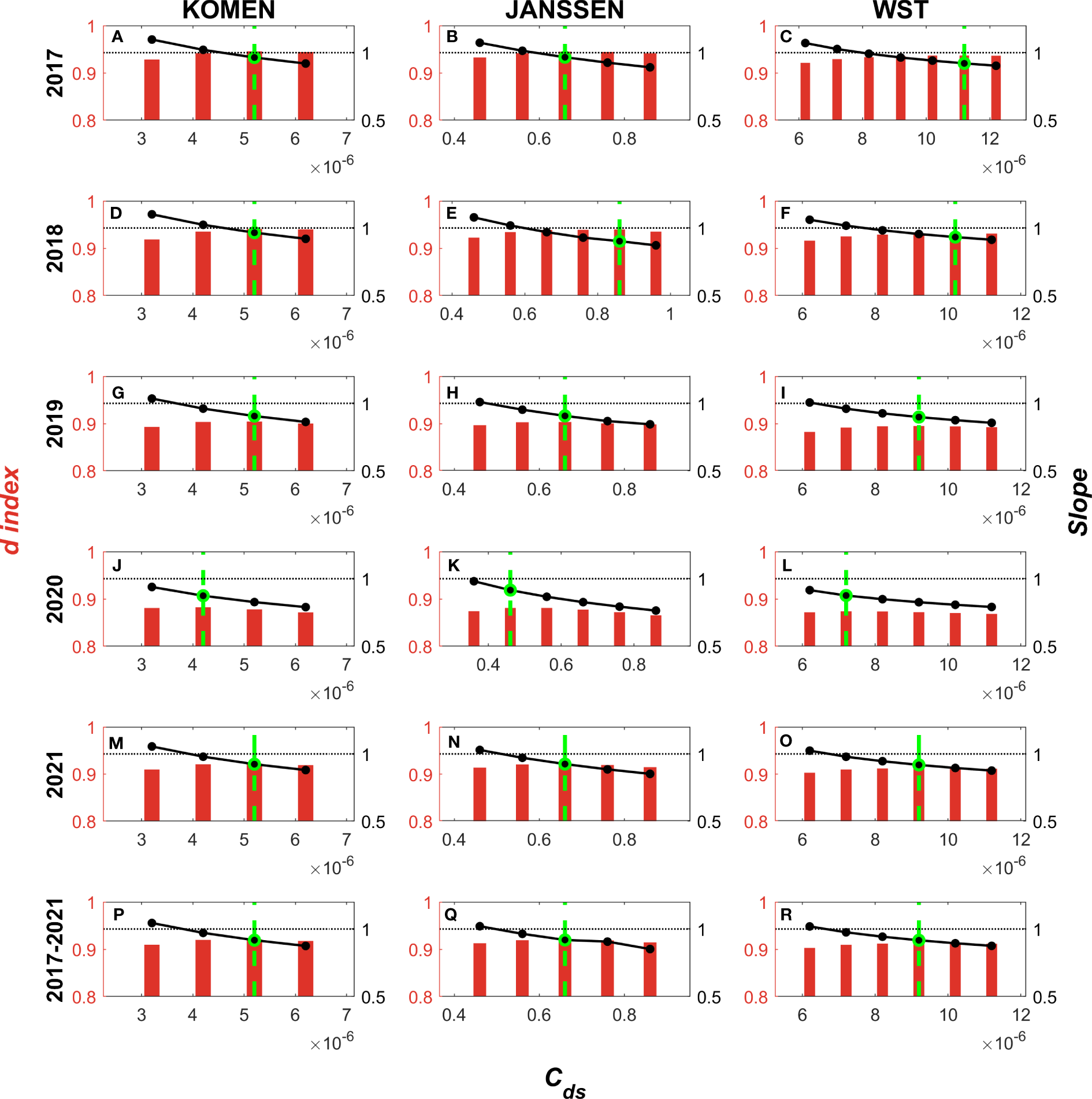
The distributions of d index and Slope for 2017 (A–C), 2018 (D–F), 2019 (G–I), 2020 (J–L), 2021 (M–O) and the five years (P–R). From left to right, (A, D, G, M, J, P) are KOMEN; (B, E, H, K, N, Q) are JANSSEN; (C, F, I, L, O, R) are WST. The crimson bars show the d index for each experiment, corresponding to the left Y-axis. The other settings are the same as in Figure 4.
Regarding the d index, the simulation performance in 2020 exhibits the poorest results, with the d index falling below 0.90 for all three schemes. When examining the d index of the optimal Cds values, the simulation performance of KOMEN and JANSSEN is superior to that of WST, even in the year with the worst simulation performance in 2020.
As highlighted in Section 4.2, the quality of the wind field in 2020 displayed fluctuations, with its Slope significantly lower than that of other years. This discrepancy indicates a severe underestimation of the actual wind field by the wind field product in 2020. Referring to Figure 5, it is evident that the optimal Cds value for 2020 is the smallest among the five years. This finding further strengthens the confirmation of the compensatory relationship between the wind errors and Cds, as elucidated in Section 4.
To address the potential impact of short-term disruptions on the overall quality of the wind field, we considered the period from 2017 to 2021 as a unit, as depicted in Figures 5P–R. Comparing the optimal Cds values for the five years to that of 2021 reveals a complete equivalence between them. In Figure 3, the Slope and d index of ERA5 for the five-year timeframe closely approximate those of 2021, providing further evidence of the direct relationship between wind errors and the optimal Cds values. Furthermore, by comparing the d index in close proximity to the optimal Cds values, we observe minimal differences among them. This finding implies that the optimal value attained for the five-year period consistently yields favorable simulation performance annually. In essence, the longer the simulation timeframe, the more accurately the main characteristics of the optimal Cds can be reflected. Therefore, a simulation duration of five years will be maintained for subsequent validation experiments.
5.3 Sensitivity to different wind fields
The preceding section focused on the optimal Cds characteristics when using ERA5 as the forcing wind field. In order to assess the generalizability of the optimal Cds features, we conducted experiments using CCMP and FNL as alternative forcing wind fields.
As shown in Figure 3, the Slope reaches the highest when the CCMP is applied, while it is the lowest for the ERA5 winds. Figure 6 provides an illustration of the optimal Cds values, showing that CCMP generally has the highest Cds values among the three wind field products, while ERA5 exhibits the lowest values. This finding provides further confirmation of the compensatory relationship between wind field errors and Cds. Remarkably, for KOMEN, it is observed that the optimal Cds values are identical across all three wind field products, at 0.52E-5. The optimal Cds range for JANSSEN is [0.66, 0.76], while for WST, it fluctuates within the range of [0.92E-5, 1.12E-5]. Similar to the seasonal and interannual characteristics, the fluctuation range of the optimal Cds among different wind field products is also minimal.
Figure 6
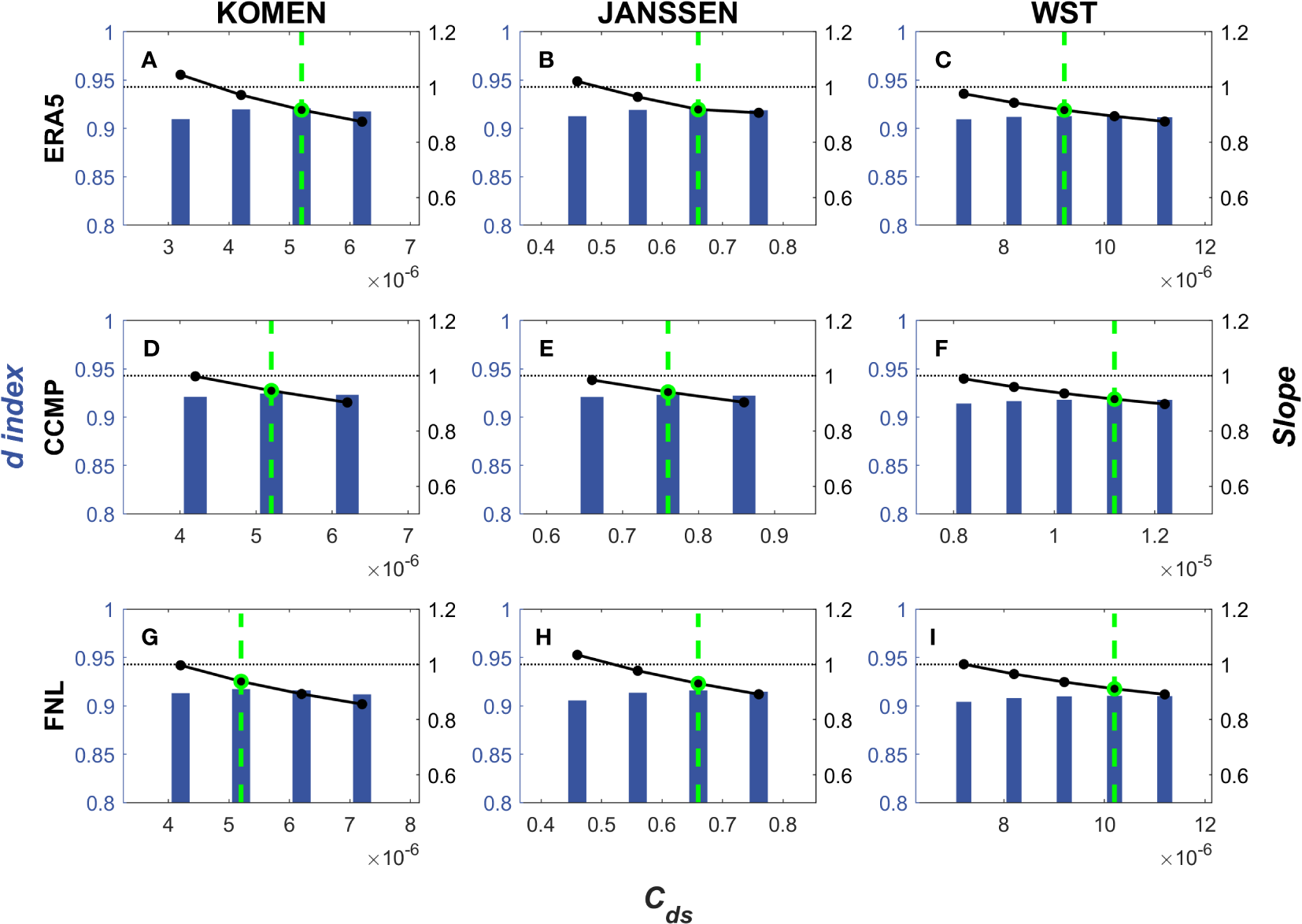
The distribution of d index and Slope of ERA5 (A–C), CCMP (D–F), and FNL (G–I). From left to right, (A, D, G) are KOMEN; (B, E, H) are JANSSEN; (C, F, I) are WST. The blue bars show the d index for each experiment, corresponding to the left Y-axis. The other settings are the same as in Figure 4.
Figure 7 presents the differences in simulation performance between the optimal Cds values and the default Cds values across all experiments. The optimal Cds values are represented by the black lines in the figure, corresponding to the right y-axis. The maximum value on the right y-axis represents the default Cds for each scheme. It is evident that the range of the optimal Cds values for all three schemes is significantly narrower compared to the default values of the model. Specifically, for the individual whitecapping dissipation schemes, the optimal Cds range is [0.42E-5, 0.52E-5] for KOMEN, [0.46, 0.86] for JANSSEN, and [0.72E-5, 1.12E-5] for WST. From the experiments conducted above, we can conclude that the variations in wind field errors across different time scales and types indeed result in fluctuations in the optimal Cds values. However, due to the overall stability of wind field errors, the optimal Cds values also fluctuate within a small range. These results demonstrate the reliability of the theoretical basis proposed in Section 4.
Figure 7
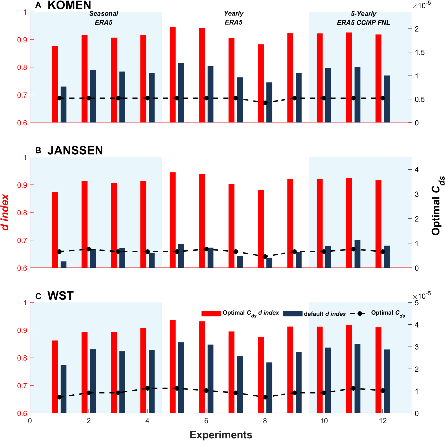
The difference in model performance between the optimal Cds and the default Cds for KOMEN (A), JANSSEN (B), and WST (C). The X-axis represents the experiment number: 1) 1–4 are seasonal results driven by ERA5; 2) 5–9 are interannual results driven by ERA5; 3) 10–12 are 5-year simulation results driven by ERA5, CCMP, and FNL. The red and dark blue bars represent the d index for the optimal Cds and the default Cds, corresponding to the left Y-axis. The dash black line shows the optimal Cds values distribution for all experiments, corresponding to the right Y-axis.
The red and dark blue bars in Figure 7 represent the d index of the optimal Cds and default Cds, respectively, corresponding to the left y-axis of the figure. It can be observed that the d index of the optimal Cds values for all three schemes is consistently around 0.90, indicating significantly improved simulation performance compared to the default values. The most notable enhancement is observed for JANSSEN with the optimal Cds values, while the improvement is minimal for WST. This finding suggests that the default value of WST exhibits the best simulation performance among the three schemes. From the previous experimental results, we have discovered that Cds values near the optimal Cds also yield excellent simulation performance. In other words, selecting any Cds value within the proposed optimal value range would result in improved simulation performance than the default value of the model.
6 Discussion
This study aims to propose a general method for determining the optimal Cds to enhance the accuracy of ocean wave simulation. However, the primary focus of this paper is on the SCS. Therefore, to determine the wider applicability of the optimal Cds intervals, two additional regions, namely the Gulf of Mexico (GoM; 98°W–78°W, 17°N–31°N) and the MS (8°W–37°E, 28°N–45°N), were selected as study areas. The GoM and the MS share similarities with the SCS, featuring complex topography and drastic variations in water depth. They also serve as vital maritime routes and regions rich in natural resources (Huerta and Harry, 2012; Appendini et al., 2013; Elkut et al., 2021; Beyramzadeh and Siadatmousavi, 2022). Therefore, choosing these areas as subjects of study holds heightened practical relevance. The time range, model settings, and observational data remained consistent with this study. Similarly, we filtered the raw data by excluding data points that were more than 5 kilometers away from the grid points. As a result, there were 44,756 valid data for the GoM and 84,272 valid data for the MS. To effectively utilize computational resources, we only used ERA5 to drive the model.
Figure 8A displays the bathymetry map for the GoM and the MS. For the GoM (Figures 8B, D, F), optimal Cds values are determined as 0.42E-5 for KOMEN, 0.46 for JANSSEN, and 0.82E-5 for WST, respectively. Similarly, for the MS (Figures 8C, E, G), the optimal Cds values for the respective schemes are 0.52E-5, 0.66, and 1.02E-5. All the optimal Cds values for both regions fall within the proposed range, demonstrating the robust applicability of the proposed viewpoint across different regions.
Figure 8
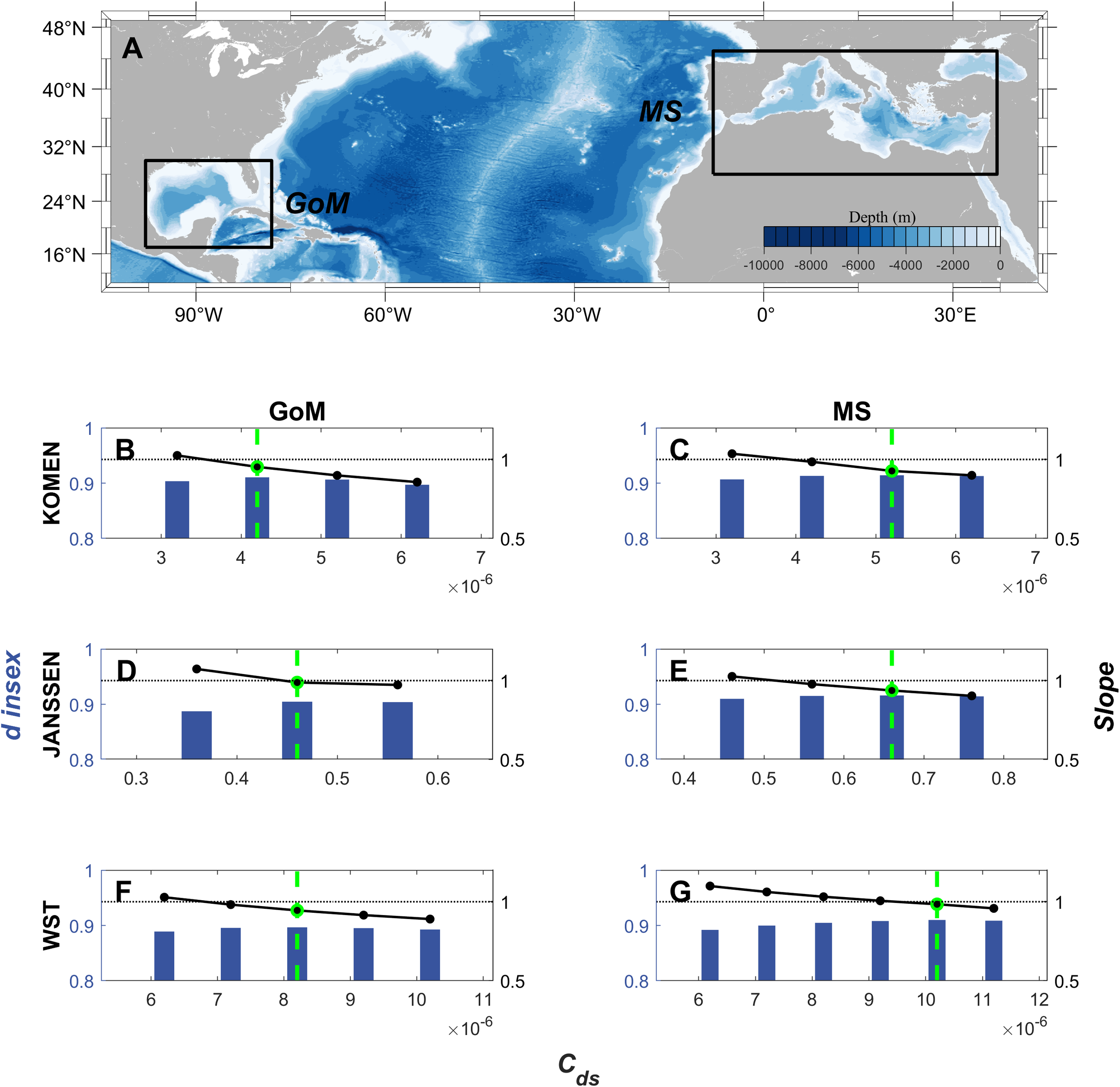
The distribution of d index and Slope in the GoM (B, D, F) and MS (C, E, G). From top to bottom, (A) is a schematic of the simulated area; (B, C) are KOMEN; (D, E) are JANSSEN; (F, G) are WST. The other settings are the same as in Figure 6.
This study primarily focuses on two wind input schemes, ST6 and YAN, in SWAN. However, SWAN offers multiple other wind input schemes to choose from. Different wind input schemes can result in variations in the energy input to the wave model (Wang and Huang, 2004; Adcock and Taylor, 2018), potentially leading to variations in the optimal Cds range. Nevertheless, the optimal Cds values will always fluctuates within a very small range.
When utilizing the optimal Cds range, two considerations must be taken into account. Firstly, our conclusions are based on a large volume of observational data. In cases where the validation dataset is insufficient or the simulation duration is too short, such as during typhoon events, the limited number of samples can lead to potential errors. Therefore, it’s essential to exercise caution when applying the optimal Cds range under these circumstances. Additionally, for nearshore wave simulations, where whitecapping dissipation no longer dominates, the contributions of bottom friction and depth-induced breaking to the dissipation process become prominent (Xu et al., 2013; Peng et al., 2023). Moreover, errors in nearshore wind fields can increase. Therefore, adjusting a single parameter alone may not yield satisfactory simulation results. In such cases, the utilization of the optimal Cds range also needs to be approached with caution. Typhoon and nearshore wave simulations hold significant research value, and these aspects will be the main focus of our future investigations.
7 Conclusion
Calibrating wave models is of paramount importance for simulating SWH, with Cds often serving as a primary calibration parameter. Nevertheless, determining the optimal Cds value is a challenging task. This study, through theoretical analysis and numerical experiments, provides a robust optimal Cds range. Within this range, the accuracy of simulated SWH for any Cds value is better than the model’s default Cds.
Specifically, we begin by revealing a direct relationship between wind errors and the optimal Cds through sensitivity experiments. Through a comprehensive evaluation of high-quality wind field products using satellite observational data, we have discovered that the errors of these wind field products are stable. This mechanism suggests that, under high-quality wind field conditions, the optimal Cds values will exhibit small fluctuations.
To verify this conjecture, we conducted a five-year wave simulation in the SCS using SWAN, covering various scenarios with different time scales and wind field types. Employing two wind input schemes (ST6 and YAN) and three whitecapping dissipation schemes (KOMEN, JANSSEN, and WST), we observed that the optimal Cds values for all three whitecapping dissipation schemes fluctuated within a narrow range. Specifically, the optimal Cds range was [0.42E-5, 0.52E-5] for KOMEN, [0.46, 0.86] for JANSSEN, and [0.72E-5, 1.12E-5] for WST. These results demonstrate the applicability of our proposed viewpoint across different time scales and wind field types. Furthermore, compared to the model’s default Cds, we found that any Cds within the optimal range had better simulation performance.
To investigate the applicability of the optimal Cds characteristics in different regions, we conducted similar experiments in the GoM and the MS using ERA5. The findings demonstrated that the optimal Cds values in these regions aligned with the suggested range, affirming the universality of this approach across a global scale.
Statements
Data availability statement
The original contributions presented in the study are included in the article/supplementary material. Further inquiries can be directed to the corresponding authors.
Author contributions
ZL: Formal Analysis, Methodology, Validation, Writing – original draft. WW: Data curation, Investigation, Visualization, Writing – review & editing. YG: Resources, Software, Writing – review & editing. FZ: Conceptualization, Methodology, Writing – review & editing. PL: Resources, Supervision, Writing – review & editing.
Funding
The author(s) declare financial support was received for the research, authorship, and/or publication of this article. This study was supported by the Major program of Laoshan Laboratory for Marine Science and Technology (Grant Number LSKJ202202903), the Hainan Provincial Joint Project of Sanya Yazhou Bay Science and Technology City (Grant Number 2021CXLH0020), the Scientific and technological projects of Zhoushan (Grant Numbers 2022C01004 and 2022C81010), the National Science Foundation of China (Grant Number 42176016) and the Shandong Provincial Natural Science Foundation (Grant Number ZR2020MD059).
Acknowledgments
We acknowledge the development team of the SWAN wave model at the Delft University of Technology. We would also like to express our gratitude to the Hainan Observation and Research Station of Ecological Environment and Fishery Resource in Yazhou Bay for their invaluable support in providing data for this study.
Conflict of interest
The authors declare that the research was conducted in the absence of any commercial or financial relationships that could be construed as a potential conflict of interest.
Publisher’s note
All claims expressed in this article are solely those of the authors and do not necessarily represent those of their affiliated organizations, or those of the publisher, the editors and the reviewers. Any product that may be evaluated in this article, or claim that may be made by its manufacturer, is not guaranteed or endorsed by the publisher.
Footnotes
1.^ https://download.gebco.net/.
2.^ https://swanmodel.sourceforge.io/.
3.^ https://cds.climate.copernicus.eu/.
4.^ https://data.remss.com/ccmp/v02.0/.
References
1
Adcock T. A. A. Taylor P. H. (2018). Ocean Wave Non-Linearity and Wind Input in Directional Seas: Energy Input During Wave-Group Focussing. American Society of Mechanical Engineers. V07BT06A052. doi: 10.1115/OMAE2018-77998
2
Akpinar A. Bingolbali B. Van Vledder G. (2016). Wind and wave characteristics in the Black Sea based on the SWAN wave model forced with the CFSR winds. OCEAN Eng.126, 276–298. doi: 10.1016/j.oceaneng.2016.09.026
3
Akpinar A. Ponce de León S. (2016). An assessment of the wind re-analyses in the modelling of an extreme sea state in the Black Sea. Dyn. Atmospheres Oceans73, 61–75. doi: 10.1016/j.dynatmoce.2015.12.002
4
Alves J. H. G. M. Banner M. L. (2003). Performance of a saturation-based dissipation-rate source term in modeling the fetch-limited evolution of wind waves. J. Phys. Oceanogr.33, 1274–1298. doi: 10.1175/1520-0485(2003)033<1274:POASDS>2.0.CO;2
5
Amarouche K. Akpınar A. Bachari N. E. I. Çakmak R. E. Houma F. (2019). Evaluation of a high-resolution wave hindcast model SWAN for the West Mediterranean basin. Appl. Ocean Res.84, 225–241. doi: 10.1016/j.apor.2019.01.014
6
Appendini C. M. Torres-Freyermuth A. Oropeza F. Salles P. López J. Mendoza E. T. (2013). Wave modeling performance in the Gulf of Mexico and Western Caribbean: Wind reanalyses assessment. Appl. Ocean Res.39, 20–30. doi: 10.1016/j.apor.2012.09.004
7
Atlas R. Hoffman R. N. Ardizzone J. Leidner S. M. Jusem J. C. Smith D. K. et al . (2011). A cross-calibrated, multiplatform ocean surface wind velocity product for meteorological and oceanographic applications. Bull. Am. Meteorol. Soc92, 157–174. doi: 10.1175/2010BAMS2946.1
8
Babanin A. V. Tsagareli K. N. Young I. R. Walker D. J. (2010). Numerical investigation of spectral evolution of wind waves. Part II: dissipation term and evolution tests. J. Phys. Oceanogr.40, 667–683. doi: 10.1175/2009JPO4370.1
9
Banner M. L. Babanin A. V. Young I. R. (2000). Breaking probability for dominant waves on the sea surface. J. Phys. Oceanogr.30, 3145–3160. doi: 10.1175/1520-0485(2000)030<3145:BPFDWO>2.0.CO;2
10
Beyramzade M. Siadatmousavi S. M. Majidy Nik M. (2019). Skill assessment of SWAN model in the red sea using different wind data. Reg. Stud. Mar. Sci.30, 100714. doi: 10.1016/j.rsma.2019.100714
11
Beyramzadeh M. Siadatmousavi S. M. (2022). Skill assessment of different quadruplet wave-wave interaction formulations in the WAVEWATCH-III model with application to the Gulf of Mexico. Appl. Ocean Res.127, 103316. doi: 10.1016/j.apor.2022.103316
12
Bingölbali B. Akpınar A. Jafali H. Vledder G. P. V. (2019). Downscaling of wave climate in the western Black Sea. Ocean Eng.172, 31–45. doi: 10.1016/j.oceaneng.2018.11.042
13
Booij N. Ris R. C. Holthuijsen L. H. (1999). A third-generation wave model for coastal regions: 1. Model description and validation. J. Geophys. Res. Oceans104, 7649–7666. doi: 10.1029/98JC02622
14
Bujak D. Lončar G. Carević D. Kulić T. (2023). The feasibility of the ERA5 forced numerical wave model in fetch-limited basins. J. Mar. Sci. Eng.11, 59. doi: 10.3390/jmse11010059
15
Cavaleri L. Abdalla S. Benetazzo A. Bertotti L. Bidlot J.-R. Breivik Ø. et al . (2018). Wave modelling in coastal and inner seas. Prog. Oceanogr.167, 164–233. doi: 10.1016/j.pocean.2018.03.010
16
Cavaleri L. Barbariol F. Benetazzo A. (2020). Wind–wave modeling: where we are, where to go. J. Mar. Sci. Eng.8, 260. doi: 10.3390/jmse8040260
17
Cavaleri L. Barbariol F. Benetazzo A. Waseda T. (2019). Ocean wave physics and modeling: the message from the 2019 WISE meeting. Bull. Am. Meteorol. Soc100, ES297–ES300. doi: 10.1175/BAMS-D-19-0195.1
18
Cavaleri L. Bertotti L. (1997). In search of the correct wind and wave fields in a minor basin. Mon. Weather Rev.125, 1964–1975. doi: 10.1175/1520-0493(1997)125<1964:ISOTCW>2.0.CO;2
19
Chen C. Sasa K. Ohsawa T. Kashiwagi M. Prpić-Oršić J. Mizojiri T. (2020). Comparative assessment of NCEP and ECMWF global datasets and numerical approaches on rough sea ship navigation based on numerical simulation and shipboard measurements. Appl. Ocean Res.101, 102219. doi: 10.1016/j.apor.2020.102219
20
Christakos K. Björkqvist J.-V. Tuomi L. Furevik B. R. Breivik Ø. (2021). Modelling wave growth in narrow fetch geometries: The white-capping and wind input formulations. Ocean Model.157, 101730. doi: 10.1016/j.ocemod.2020.101730
21
Elkut A. E. Taha M. T. Abu Zed A. B. E. Eid F. M. Abdallah A. M. (2021). Wind-wave hindcast using modified ECMWF ERA-Interim wind field in the Mediterranean Sea. Estuar. Coast. Shelf Sci.252, 107267. doi: 10.1016/j.ecss.2021.107267
22
Feng Z. Hu P. Li S. Mo D. (2022). Prediction of significant wave height in offshore China based on the machine learning method. J. Mar. Sci. Eng.10, 836. doi: 10.3390/jmse10060836
23
Günther H. Hasselmann S. Janssen P. A. E. M. (1992). The WAM Model cycle 4. Deutsches Klima Rechenzentrum. doi: 10.2312/WDCC/DKRZ_Report_No04
24
Hasselmann K. (1974). On the spectral dissipation of ocean waves due to white capping. Bound.-Layer Meteorol.6, 107–127. doi: 10.1007/BF00232479
25
Hasselmann K. Barnett T. Bouws E. Carlson H. Cartwright D. Enke K. et al . (1973). Measurements of wind-wave growth and swell decay during the Joint North Sea Wave Project (JONSWAP). Deut Hydrogr Z8, 1–95.
26
Hersbach H. Bell B. Berrisford P. Hirahara S. Horányi A. Muñoz-Sabater J. et al . (2020). The ERA5 global reanalysis. Q. J. R. Meteorol. Soc146, 1999–2049. doi: 10.1002/qj.3803
27
Huerta A. D. Harry D. L. (2012). Wilson cycles, tectonic inheritance, and rifting of the North American Gulf of Mexico continental margin. Geosphere8, 374–385. doi: 10.1130/GES00725.1
28
Hwang P. A. (2011). A note on the ocean surface roughness spectrum. J. Atmospheric Ocean. Technol.28, 436–443. doi: 10.1175/2010JTECHO812.1
29
Janssen P. A. E. M. (1992). “Consequences of the effect of surface gravity waves on the mean air flow,” in Breaking waves. Eds. BannerM. L.GrimshawR. H. J. (Berlin, Heidelberg: Springer Berlin Heidelberg), 193–198. doi: 10.1007/978-3-642-84847-6_19
30
Jiang Y. Rong Z. Li P. Qin T. Yu X. Chi Y. et al . (2022). Modeling waves over the Changjiang River Estuary using a high-resolution unstructured SWAN model. Ocean Model.173, 102007. doi: 10.1016/j.ocemod.2022.102007
31
Komen G. J. Hasselmann S. Hasselmann K. (1984). On the existence of a fully developed wind-sea spectrum. J. Phys. Oceanogr.14, 1271–1285. doi: 10.1175/1520-0485(1984)014<1271:OTEOAF>2.0.CO;2
32
Kutupoğlu V. Çakmak R. E. Akpınar A. van Vledder G. P. (2018). Setup and evaluation of a SWAN wind wave model for the Sea of Marmara. Ocean Eng.165, 450–464. doi: 10.1016/j.oceaneng.2018.07.053
33
Liu Q. Rogers W. E. Babanin A. V. Young I. R. Romero L. Zieger S. et al . (2019). Observation-based source terms in the third-generation wave model WAVEWATCH III: updates and verification. J. Phys. Oceanogr.49, 489–517. doi: 10.1175/JPO-D-18-0137.1
34
Lv X. Yuan D. Ma X. Tao J. (2014). Wave characteristics analysis in Bohai Sea based on ECMWF wind field. Ocean Eng.91, 159–171. doi: 10.1016/j.oceaneng.2014.09.010
35
Mears C. A. Scott J. Wentz F. J. Ricciardulli L. Leidner S. M. Hoffman R. et al . (2019). A near-real-time version of the cross-calibrated multiplatform (CCMP) ocean surface wind velocity data set. J. Geophys. Res. Oceans124, 6997–7010. doi: 10.1029/2019JC015367
36
Ou Y. Zhai F. Li P. (2018). Interannual wave climate variability in the Taiwan Strait and its relationship to ENSO events. J. Oceanol. Limnol.36, 2110–2129. doi: 10.1007/s00343-019-7301-3
37
Peng J. Mao M. Xia M. (2023). Dynamics of wave generation and dissipation processes during cold wave events in the Bohai Sea. Estuar. Coast. Shelf Sci.280, 108161. doi: 10.1016/j.ecss.2022.108161
38
Pierson W. J. Moskowitz L. (1964). A proposed spectral form for fully developed wind seas based on the similarity theory of S. A. Kitaigorodskii. J. Geophys. Res.69, 5181–5190. doi: 10.1029/JZ069i024p05181
39
Rogers W. E. Babanin A. V. Wang D. W. (2012). Observation-consistent input and whitecapping dissipation in a model for wind-generated surface waves: description and simple calculations. J. Atmospheric Ocean. Technol.29, 1329–1346. doi: 10.1175/JTECH-D-11-00092.1
40
Rogers W. E. Kaihatu J. M. Petit H. A. H. Booij N. Holthuijsen L. H. (2002). Diffusion reduction in an arbitrary scale third generation wind wave model. Ocean Eng.29, 1357–1390. doi: 10.1016/S0029-8018(01)00080-4
41
Roland A. Ardhuin F. (2014). On the developments of spectral wave models: numerics and parameterizations for the coastal ocean. Ocean Dyn.64, 833–846. doi: 10.1007/s10236-014-0711-z
42
Sepulveda H. H. Queffeulou P. Ardhuin F. (2015). Assessment of SARAL/altiKa wave height measurements relative to buoy, jason-2, and cryosat-2 data. Mar. Geod.38, 449–465. doi: 10.1080/01490419.2014.1000470
43
Shao Z. Liang B. Sun W. Mao R. Lee D. (2023). Whitecapping term analysis of extreme wind wave modelling considering spectral characteristics and water depth. Cont. Shelf Res.254, 104909. doi: 10.1016/j.csr.2022.104909
44
Sharma R. Chaudhary A. Seemanth M. Bhowmick S. A. Agarwal N. Verron J. et al . (2022). SARAL/AltiKa data analysis for oceanographic research: Impact of drifting and post star sensor anomaly phases. Adv. Space Res.69, 2349–2361. doi: 10.1016/j.asr.2021.12.008
45
Shi H. Cao X. Li Q. Li D. Sun J. You Z. et al . (2021). Evaluating the accuracy of ERA5 wave reanalysis in the water around China. J. Ocean Univ. China20, 1–9. doi: 10.1007/s11802-021-4496-7
46
Son D. Jun K. Kwon J.-I. Yoo J. Park S.-H. (2023). Improvement of wave predictions in marginal seas around Korea through correction of simulated sea winds. Appl. Ocean Res.130, 103433. doi: 10.1016/j.apor.2022.103433
47
Su H. Wei C. Jiang S. Li P. Zhai F. (2017). Revisiting the seasonal wave height variability in the South China Sea with merged satellite altimetry observations. Acta Oceanol. Sin.36, 38–50. doi: 10.1007/s13131-017-1073-4
48
Sun W. Liang B. Shao Z. Wang Z. (2022). Analysis of Komen scheme in the SWAN model for the whitecapping dissipation during the tropical cyclone. Ocean Eng.266, 113060. doi: 10.1016/j.oceaneng.2022.113060
49
The SWAN team . (2021a). SWAN: User Manual (SWAN Cycle III version 41.31AB). Delft Univ. Technol. Available at: https://swanmodel.sourceforge.io/.
50
The SWAN team . (2021b). SWAN: Scientific and technical documentation (SWAN Cycle III version 41.31AB). Delft Univ. Technol. Available at: https://swanmodel.sourceforge.io/.
51
The WAMDI Group (1988). The WAM model—A third generation ocean wave prediction model. J. Phys. Oceanogr.18, 1775–1810. doi: 10.1175/1520-0485(1988)018<1775:TWMTGO>2.0.CO;2
52
Umesh P. A. Behera M. R. (2021). On the improvements in nearshore wave height predictions using nested SWAN-SWASH modelling in the eastern coastal waters of India. Ocean Eng.236, 109550. doi: 10.1016/j.oceaneng.2021.109550
53
Van der Westhuysen A. J. Zijlema M. Battjes J. A. (2007). Nonlinear saturation-based whitecapping dissipation in SWAN for deep and shallow water. Coast. Eng.54, 151–170. doi: 10.1016/j.coastaleng.2006.08.006
54
Verron J. Bonnefond P. Andersen O. Ardhuin F. Bergé-Nguyen M. Bhowmick S. et al . (2021). The SARAL/AltiKa mission: A step forward to the future of altimetry. Adv. Space Res.68, 808–828. doi: 10.1016/j.asr.2020.01.030
55
Verron J. Sengenes P. Lambin J. Noubel J. Steunou N. Guillot A. et al . (2015). The SARAL/altiKa altimetry satellite mission. Mar. Geod.38, 2–21. doi: 10.1080/01490419.2014.1000471
56
Wang H. (2021) Analysis of spatial-temporal characteristics of waves and prediction of significant wave height in the South China Sea. Available at: https://kns.cnki.net/KCMS/detail/detail.aspx?dbname=CMFD202201&filename=1021879989.nh.
57
Wang W. Huang R. X. (2004). Wind energy input to the surface waves. J. Phys. Oceanogr.34, 1276–1280. doi: 10.1175/1520-0485(2004)034<1276:WEITTS>2.0.CO;2
58
Weatherall P. Tozer B. Arndt J. E. Bazhenova E. Bringensparr C. Castro C. et al . (2021). The GEBCO_2021 Grid - a continuous terrain model of the global oceans and land. NERC EDS Br. Oceanogr. Data Cent. NOC. doi: 10.5285/c6612cbe-50b3-0cff-e053-6c86abc09f8f
59
Wentz F. J. (2015). A 17-yr climate record of environmental parameters derived from the tropical rainfall measuring mission (TRMM) microwave imager. J. Clim.28, 6882–6902. doi: 10.1175/JCLI-D-15-0155.1
60
Willmott C. J. (1982). Some comments on the evaluation of model performance. Bull. Am. Meteorol. Soc63, 1309–1313. doi: 10.1175/1520-0477(1982)063<1309:SCOTEO>2.0.CO;2
61
Wu W. Li P. Zhai F. Gu Y. Liu Z. (2020). Evaluation of different wind resources in simulating wave height for the Bohai, Yellow, and East China Seas (BYES) with SWAN model. Cont. Shelf Res.207, 104217. doi: 10.1016/j.csr.2020.104217
62
Wu W. Liu Z. Zhai F. Li P. Gu Y. Wu K. (2021). A quantitative method to calibrate the SWAN wave model based on the whitecapping dissipation term. Appl. Ocean Res.114, 102785. doi: 10.1016/j.apor.2021.102785
63
Wu S. Liu J. Zhang G. Han B. Wu R. Chen D. (2022). Evaluation of NCEP-CFSv2, ERA5, and CCMP wind datasets against buoy observations over Zhejiang nearshore waters. Ocean Eng.259, 111832. doi: 10.1016/j.oceaneng.2022.111832
64
Xu F. Perrie W. Solomon S. (2013). Shallow water dissipation processes for wind waves off the mackenzie delta. Atmosphere-Ocean51, 296–308. doi: 10.1080/07055900.2013.794123
65
Yan L. (1987). An improved wind input source term for third generation ocean wave modelling. NASA Tech. ReportsN88-, 1–24.
66
Yang Z. Lin Y. Dong S. (2022). Weather window and efficiency assessment of offshore wind power construction in China adjacent seas using the calibrated SWAN model. Ocean Eng.259, 111933. doi: 10.1016/j.oceaneng.2022.111933
67
Zhai R. Huang C. Yang W. Tang L. Zhang W. (2023). Applicability evaluation of ERA5 wind and wave reanalysis data in the South China Sea. J. Oceanol. Limnol.41, 495–517. doi: 10.1007/s00343-022-2047-8
68
Zhai F. Wu W. Gu Y. Li P. Liu Z. (2021). Dynamics of the seasonal wave height variability in the South China Sea. Int. J. Climatol.41, 934–951. doi: 10.1002/joc.6707
69
Zhang X. Cheng L. Zhang F. Wu J. Li S. Liu J. et al . (2020). Evaluation of multi-source forcing datasets for drift trajectory prediction using Lagrangian models in the South China Sea. Appl. Ocean Res.104, 102395. doi: 10.1016/j.apor.2020.102395
70
Zheng Z. Ali M. Jamei M. Xiang Y. Abdulla S. Yaseen Z. M. et al . (2023). Multivariate data decomposition based deep learning approach to forecast one-day ahead significant wave height for ocean energy generation. Renew. Sustain. Energy Rev.185, 113645. doi: 10.1016/j.rser.2023.113645
71
Zieger S. Babanin A. V. Erick Rogers W. Young I. R. (2015). Observation-based source terms in the third-generation wave model WAVEWATCH. Ocean Model.96, 2–25. doi: 10.1016/j.ocemod.2015.07.014
Summary
Keywords
SWAN, whitecapping dissipation coefficient, wind errors, ERA5, SARAL
Citation
Lei Z, Wu W, Gu Y, Zhai F and Li P (2023) A general method to determine the optimal whitecapping dissipation coefficient in the SWAN model. Front. Mar. Sci. 10:1298727. doi: 10.3389/fmars.2023.1298727
Received
22 September 2023
Accepted
13 November 2023
Published
30 November 2023
Volume
10 - 2023
Edited by
Daniele Hauser, UMR8190 Laboratoire Atmosphères, Milieux, Observations Spatiales (LATMOS), France
Reviewed by
Aifeng Tao, Hohai University, China; José Pinho, University of Minho, Portugal
Updates
Copyright
© 2023 Lei, Wu, Gu, Zhai and Li.
This is an open-access article distributed under the terms of the Creative Commons Attribution License (CC BY). The use, distribution or reproduction in other forums is permitted, provided the original author(s) and the copyright owner(s) are credited and that the original publication in this journal is cited, in accordance with accepted academic practice. No use, distribution or reproduction is permitted which does not comply with these terms.
*Correspondence: Yanzhen Gu, guyanzhen@zju.edu.cn; Fangguo Zhai, gfzhai@ouc.edu.cn
Disclaimer
All claims expressed in this article are solely those of the authors and do not necessarily represent those of their affiliated organizations, or those of the publisher, the editors and the reviewers. Any product that may be evaluated in this article or claim that may be made by its manufacturer is not guaranteed or endorsed by the publisher.