Scale-dependent influence of multiple environmental drivers on estuarine macrobenthic crustaceans

Estuarine ecosystems are transitional environments, where land, freshwater, and marine ecosystems converge. Estuaries are also hotspots of ecological functioning and considered highly economically and culturally valuable for the ecosystem services they provide to humankind. However, multiple stressors (e.g., nutrient and sediment loading, pollution, climate change) are threatening the survival of estuarine organisms and therefore affecting the functions and services estuarine ecosystems provide. In this study, we investigated the influence of multiple environmental variables on long-term estuarine crustacean data across several estuaries in New Zealand. We focused on responses of specific crustacean groups and total crustacean abundance and richness to freshwater, ocean, and climate variables as drivers of change at large, medium, and fine spatial scales. Our analyses revealed that the abundance and richness of crustaceans, as well as the abundance of specific crustacean groups (i.e., Amphipoda, Decapoda, Cumacea, Tanaidacea), were influenced by unique combinations of environmental variables, resulting in scale dependent interactions. We also identified negative relationships between estuarine crustaceans and drivers, with decreased abundance and richness of crustaceans as the magnitude of drivers increased. Sea Surface Temperature (SST) and climate-related drivers (Southern Oscillation Index, SOI) were the dominant drivers affecting estuarine crustaceans, yet sediment muddiness negatively affected crustacean communities at all spatial scales assessed. Our research suggests that the combined effects of multiple environmental drivers such as increased muddiness, ocean warming, and climate change are likely to act in a concerted way to affect the health and functioning of estuarine ecosystems. The observed interactions between macrobenthic crustaceans and climatic and oceanic drivers have important implications for understanding climate change impacts on marine ecosystems and assist management and conservation efforts.

1 Introduction

Estuarine ecosystems are considered hotspots for biodiversity, productivity, and biogeochemical cycling (Thrush et al., 2013; Villnäs et al., 2019). These ecosystems provide a range of ecosystem services (e.g., coastal protection, food production, tourism) and functions (Barbier et al., 2011; Thrush et al., 2013; Rullens et al., 2019; Hillman et al., 2020; Lam-Gordillo et al., 2022b).As ecotones between the land and sea, estuarine ecosystems act as buffer zones, filtering organic matter, nutrients, and sediments inputs from terrestrial sources (Seitzinger, 1988; Villnäs et al., 2019; O’Meara et al., 2020; Lam-Gordillo et al., 2022b). However, increasing inputs of sediments, inorganic nutrients, and other pollutants and contaminants linked to anthropogenic activities such as climate change are challenging the buffering capacity of the estuaries and therefore the functions and services these ecosystems provide (Chapman, 2016; Cloern et al., 2016; Villnäs et al., 2019; Malone and Newton, 2020; Lam-Gordillo et al., 2022a).

Estuarine ecosystems worldwide are under pressure from past and ongoing changes as a result of shipping and port development, the conversion of natural habitats to land for agriculture and forestry, excessive fishing and resource extraction, and industrialisation (Cloern et al., 2016; Villnäs et al., 2019; Thrush et al., 2021). Yet, these ecosystems are not only affected by human pressures (e.g., reduction of river flows, increased nutrient loads, eutrophication, pollution), but also by natural cycles, events, and trends associated with tides, storms, and broader climatic drivers (e.g., increasing air and water temperatures, sea level rise). These types of environmental stressors can act together to affect estuarine organisms and in turn the health and functioning of estuarine ecosystems (Cloern et al., 2016; Hewitt et al., 2016; Ellis et al., 2017; Goulding et al., 2021; Thrush et al., 2021; Lam-Gordillo et al., 2022b).

Estuarine ecosystems naturally experience huge shifts in conditions over short time spans due to tidal cycles and many organisms already exist close to their tolerance limits. Environmental variables determine the distributions and structure of organisms based on these tolerances but added stressors could constrain their distributions and challenge the survival of organisms. The effects of multiple environmental variables on the abundance and distribution of estuarine organisms, as well as on the health and functioning of these ecosystems, may not be strictly additive. Multiple stressors can act in a multiplicative manner, resulting in greater than expected (synergistic) or lower than expected (antagonistic) effects relative to additive combinations of individual stressor effects (Thrush et al., 2008b; Ellis et al., 2017; Carrier-Belleau et al., 2021; Clark et al., 2021). These multi-stressor interactions are predicted to increase as climate change (sea-level rise, altered rainfall patterns, and increased air and water temperatures) continues to unfold (Gunderson et al., 2016; Ellis et al., 2017; Clark et al., 2021). Understanding the interactions of changing environmental variables as drivers of estuarine communities is critical to inform policy and management to ensure healthy estuarine ecosystems (Simeoni et al., 2023). However, the influence of multiple stressors on estuarine communities is difficult to characterise, leading to uncertainties on predictions of community change and the consequent effects on ecosystem functioning (Thrush et al., 2008b; Hewitt et al., 2016; Ellis et al., 2017; Clark et al., 2021; Lam-Gordillo et al., 2021; Thrush et al., 2021).

Crustaceans, such as amphipods, cumaceans, decapods, isopods, and tanaids, represent one of the most abundant and important groups of benthic macrofauna (Sánchez-Moyano and García-Asencio, 2010; Medina-Contreras et al., 2022; De Grave et al., 2023; Nozarpour et al., 2023). These organisms have been recognised as effective bioindicators for assessing environmental change due to their sensitivity to various anthropogenic and natural disturbances (Borja et al., 2000; Dauvin et al., 2006; Sánchez-Moyano and García-Asencio, 2010). Crustaceans are also key contributors to the functioning of estuarine ecosystems (e.g., Needham et al., 2011; Needham et al., 2013; Agusto et al., 2022; Nozarpour et al., 2023). For example, crustaceans are involved in trophic dynamics transferring energy and matter from lower to higher trophic levels as food source for fish and birds (Zetina-Rejon et al., 2003; Bui and Lee, 2014; Medina-Contreras et al., 2022). These organisms also alter the sedimentary environment (e.g., topography, biogeochemistry, particle size) through biological processes such as bioturbation (Lohrer et al., 2004a; Needham et al., 2011; Needham et al., 2013; Fanjul et al., 2015; Agusto et al., 2022). Bioturbating crustaceans rework the sediment (e.g., bioirrigation, bioventilation), promoting sediment oxygenation, which ultimately enhances microbial activity responsible for organic matter decomposition and nutrient cycling (Welsh, 2003; Lohrer et al., 2004a; Kristensen et al., 2012; Lam-Gordillo et al., 2022a).

Crustaceans are prominent among taxa affecting ecosystem functioning (e.g., Nozarpour et al., 2023), and are sensitive to natural and anthropogenic disturbances (e.g., Borja et al., 2000). With case study analyses of crustaceans, we can improve our understanding of how coastal ecosystems respond to increasing temperatures, sea level rise, nutrient enrichment, pollution, and in general, how the crustacean communities inhabiting estuarine ecosystems respond to the influence of multiple stressors.

In recent decades, most studies of estuarine macrofauna have focused on evaluating individual effects of single stressors, while there has been less research assessing the influence of multiple stressors on estuarine macrobenthic communities (e.g., Thrush et al., 2008b; Ellis et al., 2017; Clark et al., 2021). Here we leveraged the availability of high-quality estuarine time-series data from three sites in each of three estuaries to investigate the influence of multiple environmental variables on long-term estuarine crustacean data across three different estuaries in New Zealand. We focused on (i) evaluating responses of crustacean communities to five environmental variables at large, medium, and fine scales, and (ii) assessing the influence of these multiple drivers on specific crustacean taxa groups. We hypothesised that (1) crustaceans will respond to multiple environmental predictors more often than to single predictors, (2) the influence of multiple drivers will be spatial scale dependent, and (3) specific crustacean groups will have differential responses to multiple drivers.

2 Materials and methods

2.1 Study area

Crustacean data were collected from nine sites total, with three sites in each of three estuaries (Kaipara: KaiB, KKF, NPC, Mahurangi: HL, JB, MH, and Manukau: AA, CB, CH) located on the North Island of New Zealand (Figure 1; Table 1). Kaipara Harbour opens to the Tasman Sea on the west coast and is one of the largest estuaries in the southern hemisphere, covering ~947 km² including vast extents of seagrass habitat (Heath, 1975; Pine et al., 2015; Bulmer et al., 2016). Recent intensification of agriculture and urban development in the catchment of the estuary has contributed to increased sediment loads and decreased water clarity (Ellis et al., 2004; Bulmer et al., 2016). Mahurangi Harbour, 24.7 km², is a relatively small estuary on the east coast (Thrush et al., 2008a; Oldman et al., 2009) with intertidal flats ranging from fine muddy sediments at the head of the harbour to coarse sands near the mouth. Pastoral farming, lifestyle blocks, and forestry occur in the catchment (Gibbs et al., 2005; Thrush et al., 2008a; Oldman et al., 2009). Manukau Harbour, to the south of Kaipara Harbour on the west coast, is the second largest estuary in New Zealand at 368 km² (Heath, 1975). It is a shallow estuary with a highly developed branching channel system and a mixture of habitats including intertidal mudflats, mangrove stands, and saltmarshes (Gorman and Neilson, 1999; Green et al., 2000; Bastakoti et al., 2019). Although adjacent to Auckland, New Zealand’s largest city, the catchments draining into Manukau Harbour are small relative to estuary size and predominantly rural/pasture. All of the sites sampled in each estuary are Auckland Council ecological monitoring sites (Drylie, 2021). As such, the sites were selected for their relative similarity in terms of elevation relative to chart datum (mid-intertidal) and salinity at high tide (usually >32 PSU). However, sediment characteristics at each site varied from ‘‘muddy’’ to ‘‘sandy’’, often related to position of sites in upper versus lower estuary, respectively.

FIGURE 1

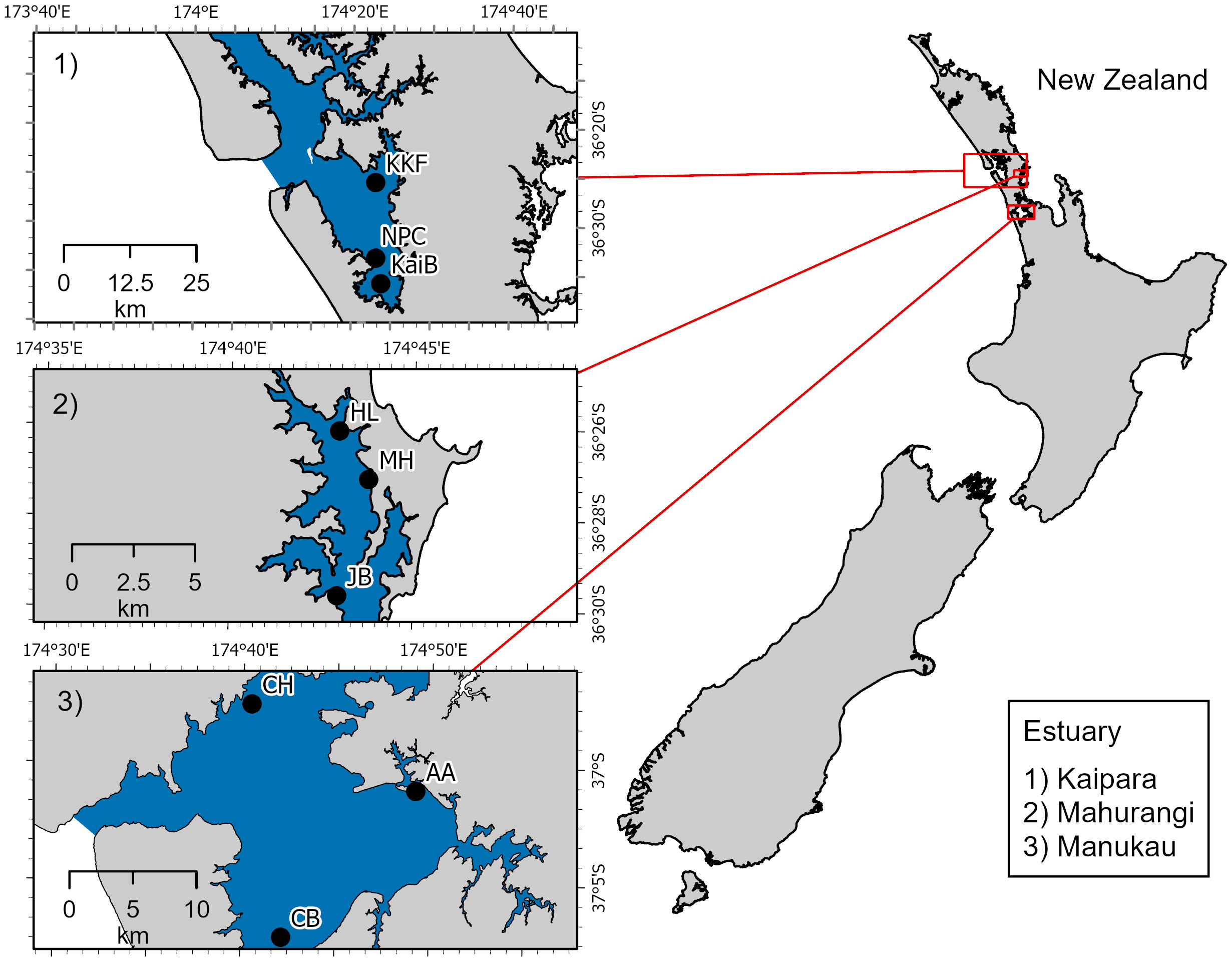
Figure 1 Map of the study area showing the nine sites across three estuaries in New Zealand from where crustacean samples were collected.

TABLE 1

Table 1 Summary details of the macrobenthic and environmental data used in this study.

2.2 Data collection

2.2.1 Biological data

Crustacean data were retrieved from a long-term macrobenthic dataset (1989-2022) held by Auckland Council to assess the ecological health of estuaries. Collection of macrobenthic organisms, processing of samples, and sorting and identifications has followed standard protocols (Robertson et al., 2002; Hewitt et al., 2014) and strict quality assurance/quality control procedures (Hewitt et al., 2014; Greenfield et al., 2023), providing high confidence in the validity of data comparisons over time. Sampling of macrobenthic fauna was performed three-monthly from 2009 to 2022, years in which all 9 sites in the three estuaries were sampled (Table 1). Briefly, at each of the sampling sites, 12 replicate sediment samples for assessing macrobenthic fauna were collected using a hand-held PVC corer (13 cm diameter by 15 cm depth), sieved through a 0.5 mm mesh size, and preserved in 70% isopropanol. Benthic macrofauna were sorted, identified to the lowest possible taxonomic level (usually genus or species), and counted.

2.2.2 Environmental drivers

Five environmental variables with the potential to influence estuarine crustacean communities were available for analysis. All relate in some degree to anthropogenic activities, but the degree to which they are deleterious or beneficial often depends on magnitude and context. The five variables assessed were sediment chlorophyll a content (Chl-a); sediment organic matter content (OM); sediment mud content (muddiness, percent dry weight of silt and clay particles <63 um); sea surface temperature along the coast outside each estuary mouth (SST, degrees Celcius); and Southern Oscillation Index value (SOI, a general indicator of climate variability).

Chl-a is a photosynthetic pigment found in marine plants that is used as a proxy for soft-sediment microphytobenthos abundance. Microphytobenthos is an important source of labile food for macroinvertebrate crustaceans. In situ photosynthetic oxygen production by microphytobenthos can increase surface sediment oxygenation levels and biogeochemical rates (e.g., organic matter degradation, nitrification-denitrification). However, very high sediment Chl-a and organic matter levels are indicative of eutrophication, resulting from excessive nutrient loading from catchments and point sources. Microbially mediated organic matter remineralisation can deplete the dissolved oxygen in sediment pore water and contribute to toxic concentrations of ammonium and hydrogen sulphide.

Increased muddiness, resulting from increases in catchment-derived fine sediments, has had major impacts on the health and functioning of estuaries in New Zealand (Thrush et al., 2004). Estuary sedimentation is naturally high in New Zealand due to high rainfall and steep topography (Hicks et al., 2019), but changes in land-use have elevated soil erosion and export rates drastically relative to pre-human times (Hunt, 2019). Inverse relationships between sediment muddiness and macrofaunal abundance, richness and diversity are relatively well documented in New Zealand estuaries (Thrush et al., 2003b; Lohrer et al., 2004b; Lohrer et al., 2006; Lohrer et al., 2012; Thrush et al., 2017). Many anthropogenic contaminants bind to and are transported by fine sediment particles, and muddiness is often strongly correlated with sediment organic matter content (with fine sediments providing proportionally more surface area for the attachment of microbes than larger particles) (Douglas et al., 2018).

Climate change manifests locally in a variety of ways. For estuaries, this can be changes in prevailing winds, rainfall, and temperatures, which can affect exposure to wind-waves, turbidity, and heat stress and desiccation at low tide. There is worldwide concern about marine heat waves (Oliver et al., 2018; Oliver et al., 2021; Xu et al., 2022), including in New Zealand, where anomalously warm years have been occurring more often recently (Oliver et al., 2018; Behrens et al., 2022). Yet is possible that increasing sea surface temperatures may positively influence benthic macroinvertebrate growth and reproduction up to a point, whereafter negative impacts may ensue. We used both sea surface temperatures (SST) and the Southern Oscillation Index (SOI) as potential predictors of macroinvertebrate crustaceans in our analysis. SOI is a measure of pressure variability between Tahiti and Darwin, Australia, associated with changes in weather and ocean current patterns worldwide. It is the index used to track the strength of El Niño (warm)/La Niña (cold) conditions. By definition, the SOI should not monotonically increase or decrease over time but will instead oscillate back and forth between positive and negative phases (occurring roughly every 2 to 7 years).

Methodological details for processing of Chl-a, OM, and grain size samples are described in full elsewhere (Douglas et al., 2017; Douglas et al., 2018; Drylie, 2021). Briefly, sediment samples for Chl-a, OM, and sediment grain size were collected using a smaller PCV corer (26 mm diameter, 20 mm deep core). Sediment from each small core was homogenised and sub-sampled for analysis of Chl a, OM, and sediment grain size. Chl-a was extracted from freeze dried sediments by boiling in 90% ethanol. The extract was measured spectrophotometrically, and an acidification step was included to separate degradation products (phaeophytin) from Chl-a (Sartory, 1982). Organic matter content was determined by drying the sediment at 60°C for 48 h and then combusting it at 400°C for 5.5 h, with OM expressed as percent dry weight lost on ignition. For sediment grain size, samples were homogenised and then digested in ~ 9% hydrogen peroxide until frothing ceases. Samples were wet sieved through 2000 µm, 500 µm, 250 µm and 63 µm mesh sieves. Pipette analysis was used to separate the <63 µm fraction into >3.9 µm and ≤3.9 µm. All fractions are then dried at 60°C until a constant weight is achieved (fractions are weighed at ~ 40 h and then again at 48 h) to obtain the percentage weight of gravel/shell hash (>2000 µm), coarse sand (500–2000 µm), medium sand (250–500 µm), fine sand (62.5–250 µm), silt (3.9–62.5 µm) and clay (≤3.9 µm).

Monthly SOI values were freely obtainable from the National Oceanographic and Atmospheric Administration - NOAA (https://www.cpc.ncep.noaa.gov). The same SOI time-series data were applied to all estuaries, as they are global scale metrics. Sea Surface Temperature (SST) data were obtained for each individual studied site. Monthly SST values for each site were generated from satellite imagery (Ocean Color - https://oceancolor.gsfc.nasa.gov) by extracting point-values from the grid-cell encompassing or closest to each site within each estuary studied.

2.3 Data analysis

To elucidate the patterns in the selected environmental variables over time, trend line analyses were performed for Chl-a, OM, Mud content, SOI, and SST individually. Linear regressions were performed and plotted using the package “ggpubr” (Kassambara, 2020) in R software (R-Core-Team, 2022).

To evaluate the influence of multiple predictors on estuarine crustaceans, we followed a spatial scale-based (i.e., large, medium, and fine scale) approach using Generalised Linear Models (GLMs). For the large scale (region), we used all the data available and evaluated the influence of all predictors on the abundance and richness of crustaceans, and the specific crustacean groups Amphipoda, Decapoda, Cumacean, and Tanaidacea. For the medium scale (estuary scale), we evaluated the influence of the multiple predictors on the abundance and richness of crustaceans, and specific crustacean groups, but separating all data by estuary (i.e., n=3). Lastly, for the fine scale (site scale) we evaluated the influence of all predictors on the abundance of estuarine crustaceans at each individual study site (n=9). All GLMs were constructed based on negative binomial regression model using the package “MASS” (Venables and Ripley, 2002). The GLM offers several advantages over conventional distance-based multivariate approaches, including accounting for species relationships, counts of rare species with zero-inflated abundance data, and the mean-variance relationship. Partial regression residual plots and forest (estimates) plots were created to investigate direct relationships between predictors and responses using the package “car” (Fox and Weisberg, 2019) and “sjPlot” (Lüdecke, 2023) respectively. Forest plots are a useful graphical means of summarising outcomes from GLMs, indicating the significance and direction (i.e., increase or decrease) of interactions between predictor and response variables. We did not use backward, forward, or stepwise techniques to determine final models, rather we used all five explanatory variables in each GLM and examined coefficient p-values to determine their significance. All the GLM and derived plots were performed using R software (R-Core-Team, 2022).

3 Results

A total of 56,751 crustacean organisms were collected from 2009 to 2022. The highest mean total abundance of crustaceans across sites and times in a harbour was recorded in Manukau Harbour (178 crustaceans), followed by Mahurangi (102 crustaceans), with the lowest mean total abundance recorded in Kaipara Harbour (60 crustaceans). Similarly, the highest mean total richness of crustaceans was found in Manukau Harbour (9 taxa), with the lowest richness found in Kaipara (7 taxa). At site level, CH (Manukau) was the site that showed the highest mean total abundance of crustaceans (302 crustaceans). The lowest mean total abundance was recorded at KaiB (Kaipara – 26 crustaceans). In terms of crustacean richness, JB (Mahurangi) showed the highest mean total richness (14 taxa), while the lowest mean total richness was observed at KaiB (5 taxa).

3.1 Trends in environmental drivers over time

Chlorophyll a (Chl-a) decreased over time at six of the nine sites studied (Table 2, Figure 2). In Kaipara Harbour, Chl-a increased at KaiB site, the site furthest from the estuary mouth, but decreased over time at the other sites (KKF and NPC; Table 2, Figure 2A). Similar trends were observed in Mahurangi Harbour: Chl-a increased over time at sites far from the estuary mouth (HL and MH) but decreased at the outermost site, JB. (Table 2, Figure 2B). In Manukau Harbour, Chl-a decreased over time at all the sites (Table 2, Figure 2C).

TABLE 2

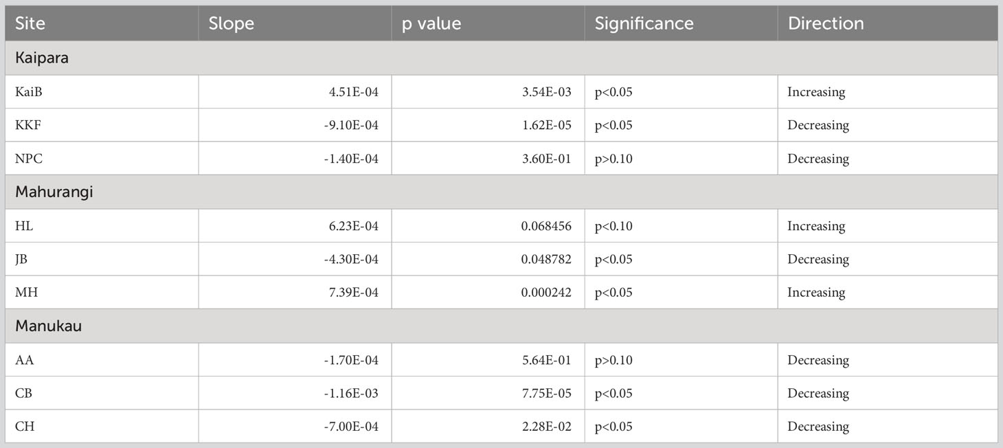
Table 2 Summary results of regression line analyses showing trends in Chlorophyll a (Chl-a) over time at each site.

FIGURE 2

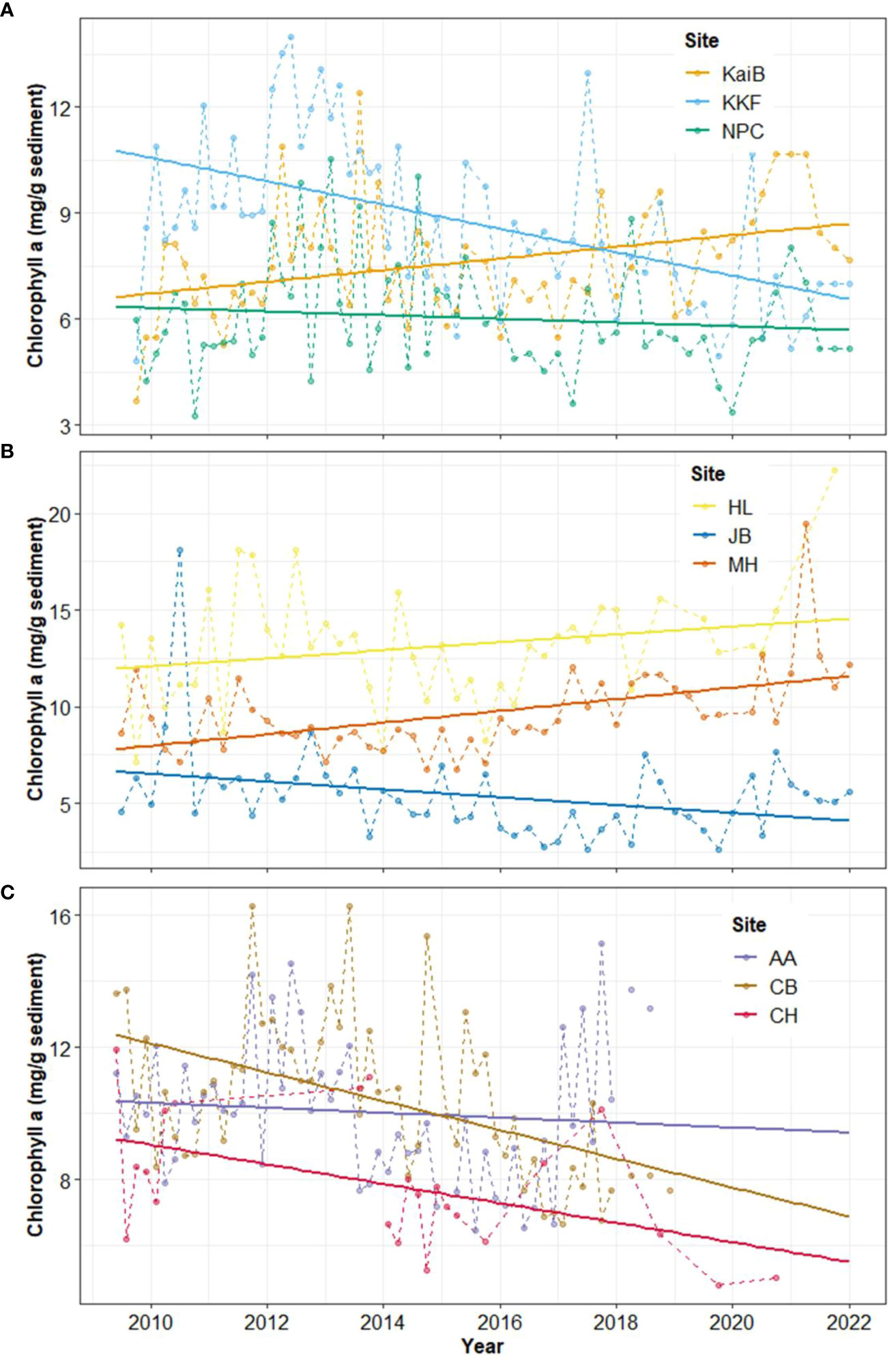
Figure 2 Time-series and linear trend analysis of Chlorophyll a in (A) Kaipara, (B) Mahurangi, and (C) Manukau estuary. Points and dashed lines depict data values and solid lines represent the regression. Note different Y-axis scales.

In contrast to Chl-a, organic matter content (OM) significantly increased over time (Table 3, Figure 3). In Kaipara and Mahurangi Harbours, OM increased at all study sites (Table 3, Figures 3A, B). OM was low in Manukau Harbour compared to the other estuaries, with increases detected at AA and CH. Site CB in Manukau harbour was the only site exhibiting a decrease in OM over time (Table 3, Figure 3C).

TABLE 3

Table 3 Summary results of the regression line analyses showing trends in sediment organic matter content (OM) over time at each site.

FIGURE 3

Figure 3 Time-series and linear trend analysis of sediment organic matter content in in (A) Kaipara, (B) Mahurangi, and (C) Manukau estuary. Points and dashed lines depict data values and solid lines represent the regression. Note different Y-axis scales.

Sediment mud content also generally increased over time in the study estuaries (Table 4, Figure 4). Mud content increased in all sites in Kaipara Harbour (Table 4, Figure 4A), at AA and CH in Manukau Harbour (Table 4, Figure 4C), and at HL in Mahurangi Harbour (Table 4, Figure 4B).

TABLE 4

Table 4 Summary results of regression line analyses showing trends in sediment mud content over time at each site.

FIGURE 4

Figure 4 Time-series and linear trend analysis of sediment mud content in (A) Kaipara, (B) Mahurangi, and (C) Manukau estuary. Points and dashed lines depict data values and solid lines represent the regression. Note different Y-axis scales.

Long-term data (1984-2022) of the Southern Oscillation Index (SOI) revealed high variation of warm (El Niño) and cold (La Niña) climate (Figure 5). Analysis of the 1984-2022 data record indicates increasing SOI over time, with longer periods of warmer (El Niño) climate (Figure 5A). However, for the more recent period (i.e., the 2009-2022 timeframe of this study), SOI is trending downward, indicting longer and wider periods of cold (La Niña) climate (Figure 5B).

FIGURE 5

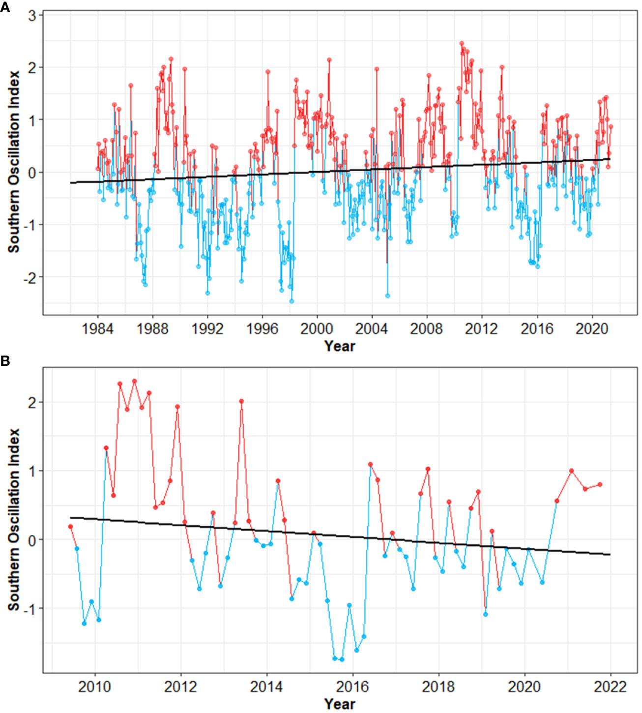
Figure 5 Time-series and linear trend analysis of the Southern Oscillation Index. (A) Long-term values (1984-2022), and (B) time frame of this study. Regression lines are indicated by solid black lines. Warm periods (El Niño) are in red, and cold periods (La Niña) in blue. Note different X-axis scales.

Seasonal cycles in Sea Surface Temperature (SST) were apparent at all sites, with warmer SST in austral summer and colder SST in austral winter (Figure 6). Linear trend analyses indicated an increase in SST of roughly 1°C at most study sites, with decreases through time at just two sites (HL and CH; Table 5, Figure 6).

FIGURE 6

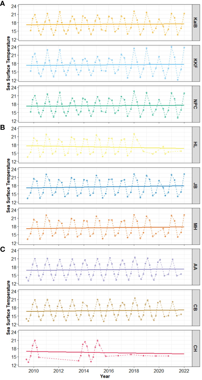
Figure 6 Time-series and linear trend analysis of Sea Surface Temperature in (A) Kaipara, (B) Mahurangi, and (C) Manukau estuary. Solid lines show the regression line, and points and dashed lines showed the data values. Right-hand Y-axis denotes site names.

TABLE 5

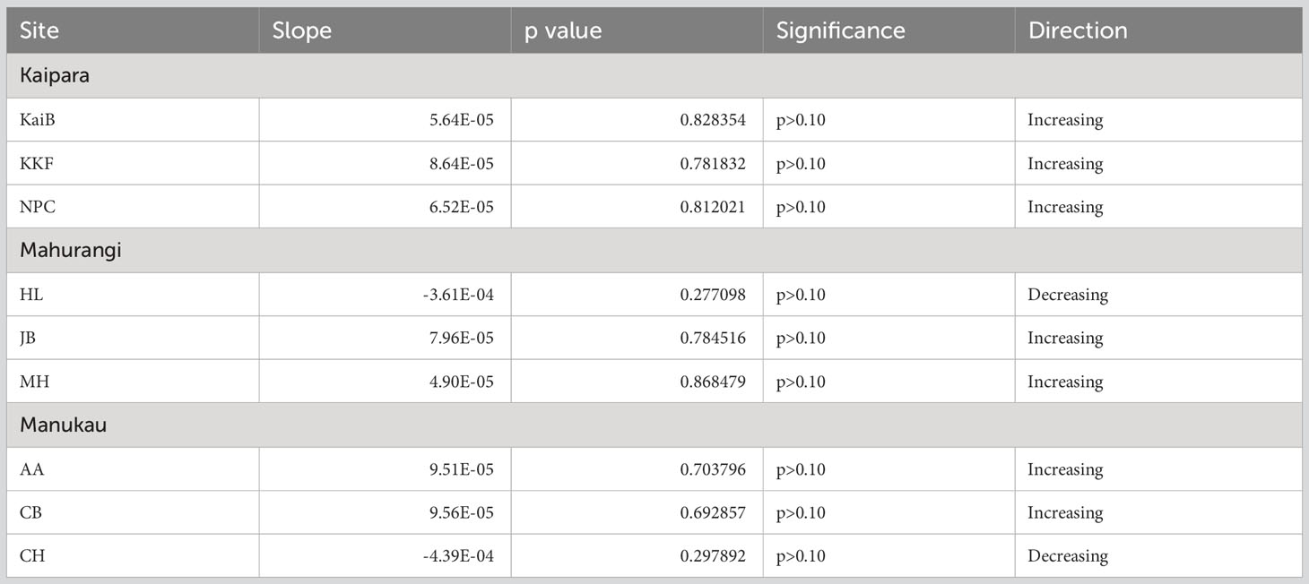
Table 5 Summary results of regression line analyses showing Sea Surface Temperature (SST) over time at each site.

3.2 Large (region) scale

GLM results showed how multiple environmental variables influenced crustacean communities at the large spatial scale, i.e., all the estuaries together (Figure 7, Supplementary Table 1). Crustacean abundance was significantly influenced by four variables (Figure 7A). Three of the four variables (SOI, SST and mud content) were inversely related to the abundance of crustaceans, i.e., with crustacean abundance decreasing as SOI, SST and mud content increased (Figure 7A, Supplementary Figure 1, Supplementary Table 1). Crustacean richness was influenced by SOI, mud and organic content (Figure 7B) and, as above, richness tended to decrease with increasing SOI and mud content (Figure 7B, Supplementary Figure 2, Supplementary Table 1).

FIGURE 7

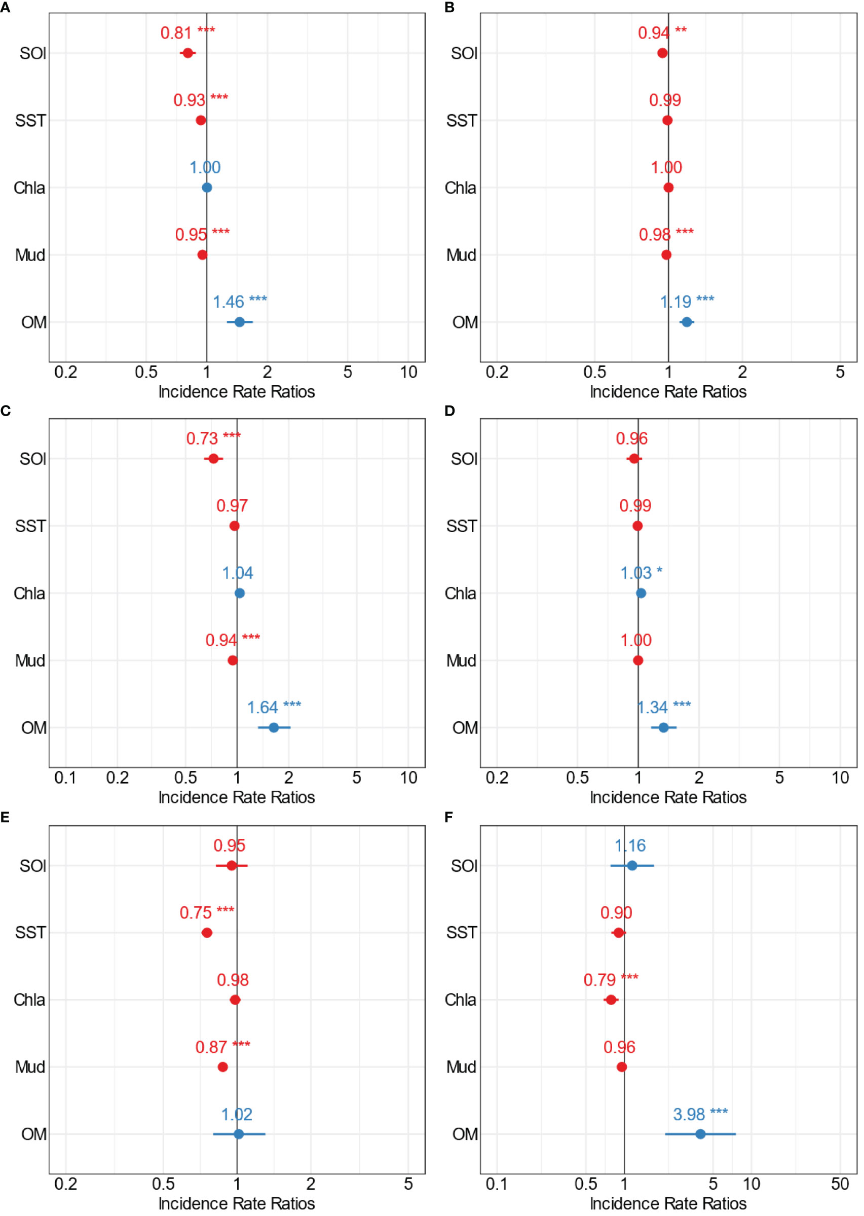
Figure 7 Forest plots summarising the outcomes from GLMs for the large-scale analysis showing the point estimates (Incidence Rate Ratios) for the relationships between multiple stressors and (A) total crustacean abundance, (B) crustacean richness, (C) Amphipoda, (D) Decapoda, (E) Cumacean, and (F) Tanaidacea abundance. The colour indicates positive (blue) and negative (red) significant (*p=0.5; **p=0.01; ***p=0.001) interactions of the point estimates.

The crustacean groups Amphipoda, Decapoda, Cumacean, and Tanaidacea were significantly influenced by distinct combinations of multiple environmental predictors (Figures 7C-F). Amphipoda abundance decreased with increasing SOI and mud content (Figure 7C, Supplementary Figure 3, Supplementary Table 1), while the abundance of Decapoda increased with increasing Chl-a and OM (Figure 7D, Supplementary Figure 4, Supplementary Table 1). SST and mud content influenced the abundance of Cumacea, showing a trend of decreasing abundance with increasing SST and mud content (Figure 7E, Supplementary Figure 5, Supplementary Table 1). A similar inverse relationship was found with Tanaidacea abundance and Chl-a (decreasing abundance with increasing Chl-a; Figure 7E, Supplementary Figure 6, Supplementary Table 1).

Organic content influenced all of the crustacean variables analysed with the exception of Cumacea abundance. Increases in OM generally resulted in increased crustacean abundance and richness, and increased abundance of Amphipoda, Decapoda, and Tanaidacea (Figure 7E, Supplementary Figures 1–6, Supplementary Table 1).

3.3 Medium (estuary) scale

Crustacean communities were also influenced by estuarine-scale variation in environmental predictors (Figures 8–10, Supplementary Tables 1–4). For Kaipara Harbour, the GLM results showed the abundance of crustaceans to be significantly influenced by SOI, SST, mud and organic content (Figure 8A). Similar to the large-scale patterns, crustacean abundance decreased with increases in SOI, SST and mud content (Figure 8A, Supplementary Figure 7, Supplementary Table 2). Crustacean richness in Kaipara Harbour was influenced by fewer variables, increasing with Chl-a and decreasing with mud content but showing no relationship to SOI, SST or organic matter content (Figure 8B, Supplementary Figure 8, Supplementary Table 2). Amphipoda abundance in Kaipara followed the same pattern as crustacean abundance, i.e., decreasing with increasing SOI, SST and mud content (Figure 8C, Supplementary Figure 9, Supplementary Table 2) and increasing with OM. Decapoda abundance was also influenced by multiple variables, showing an increase in abundance with increasing Chl-a, mud, and OM (Figure 8D, Supplementary Figure 10, Supplementary Table 2). Cumacea abundance was inversely correlated with SOI, SST and mud content (Figure 8E, Supplementary Figure 11, Supplementary Table 2), while Tanaidacea abundance was not influenced by any of the multiple stressors assessed (Figure 8F, Supplementary Figure 12, Supplementary Table 2). Overall, mud content was the stressor that influenced the largest number of crustacean variables in Kaipara Harbour, with abundance and richness tending to decrease with increasing mud content in sediments.

FIGURE 8

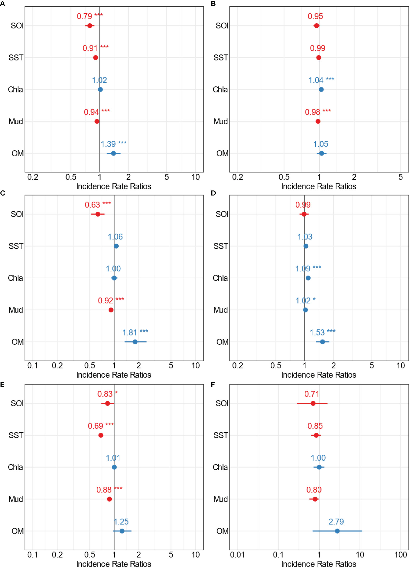
Figure 8 Forest plots summarising the outcomes from GLMs for Kaipara estuary (medium scale) showing the point estimates (Incidence Rate Ratios) for the relationships between multiple stressors and (A) total crustacean abundance, (B) crustacean richness, (C) Amphipoda, (D) Decapoda, (E) Cumacean, and (F) Tanaidacea abundance. The colour indicates positive (blue) and negative (red) significant (*p=0.5; **p=0.01; ***p=0.001) interactions of the point estimates.

FIGURE 9

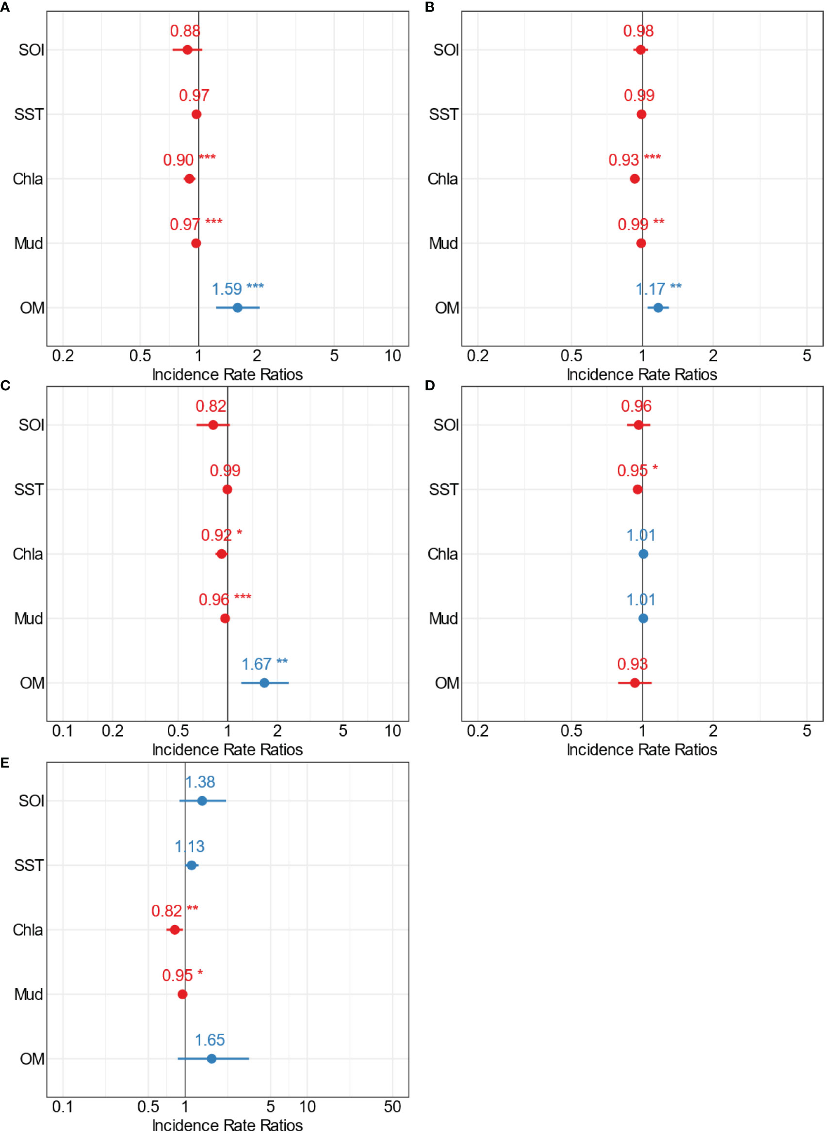
Figure 9 Forest plots summarising the outcomes from GLMs for Mahurangi estuary (medium scale) showing the point estimates (Incidence Rate Ratios) for the relationships between multiple stressors and (A) total crustacean abundance, (B) crustacean richness, (C) Amphipoda, (D) Decapoda, and (E) Cumacean abundance. The colour indicates positive (blue) and negative (red) significant (*p=0.5; **p=0.01; ***p=0.001) interactions of the point estimates.

FIGURE 10

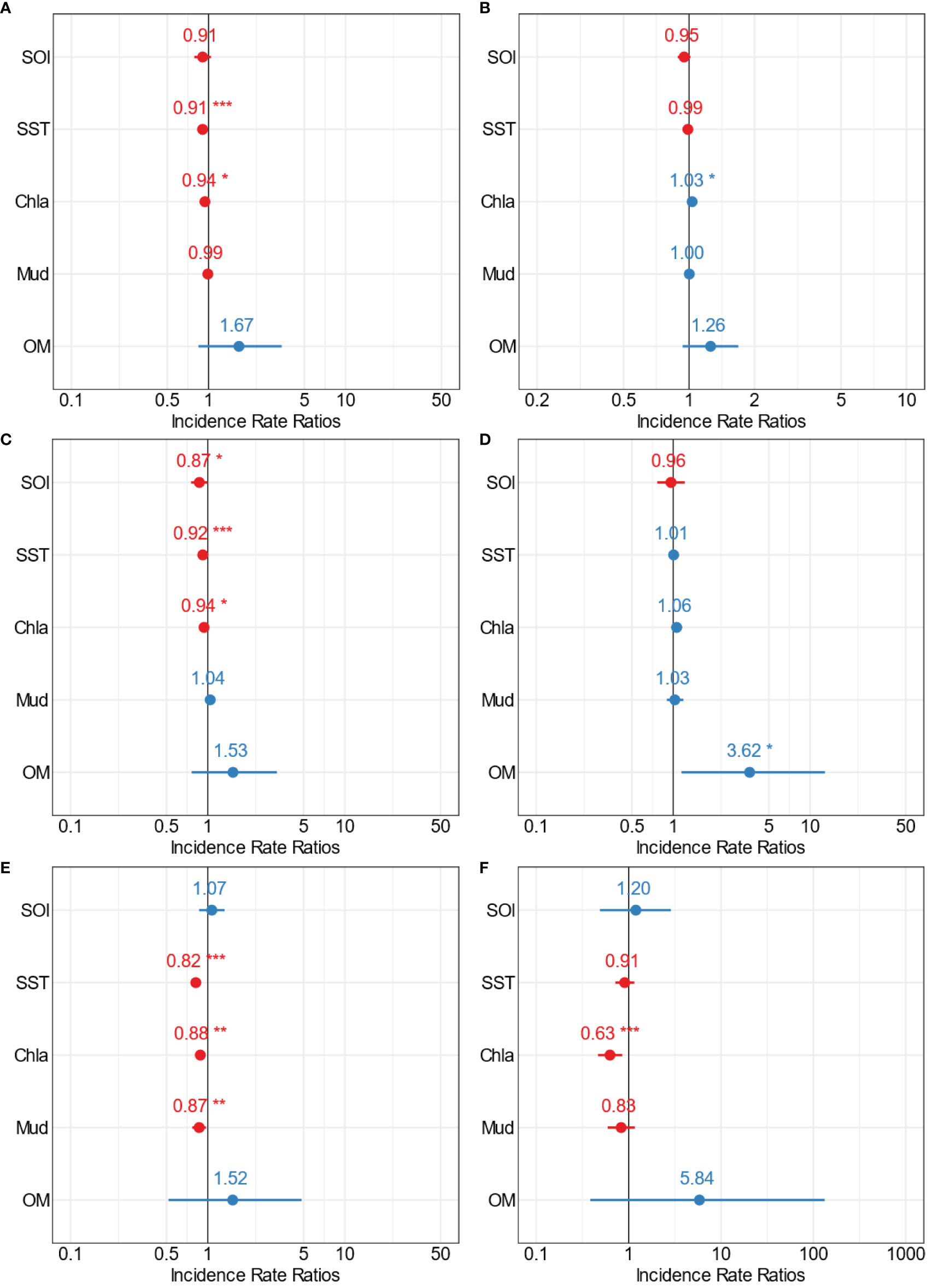
Figure 10 Forest plots summarising the outcomes from GLMs for Manukau estuary (medium scale) showing the point estimates (Incidence Rate Ratios) for the relationships between multiple stressors and (A) total crustacean abundance, (B) crustacean richness, (C) Amphipoda, (D) Decapoda, (E) Cumacean, and (F) Tanaidacea abundance. The colour indicates positive (blue) and negative (red) significant (*p=0.5; **p=0.01; ***p=0.001) interactions of the point estimates.

Results from Mahurangi Harbour were similar to those in Kaipara. For example, crustacean abundance and richness were significantly influenced by Chl-a, mud, and OM (Figures 9A, B, Supplementary Table 3). Both of these response variables decreased when Chl-a and mud content increased (Figures 9A, B, Supplementary Figures 13, 14, Supplementary Tables 1–3). Chl-a, mud, and OM were also significant predictors of Amphipoda abundance (Figure 9C, Supplementary Figure 15, Supplementary Tables 1–3). Decapoda abundance in Mahurangi Harbour was only influenced by one environmental variable, SST (negatively; Figure 9D, Supplementary Figure 16, Supplementary Table 3), whereas Cumacea abundance was influenced by two different environmental variables, Chl-a and mud content (both negatively, Figure 9E, Supplementary Figure 17, Supplementary Table 3). As was the case in Kaipara Harbour, mud content was the environmental variable with the most pervasive negative effects on crustacean responses in Mahurangi Harbour.

The patterns observed in Manukau Harbour were rather different to those in Kaipara and Mahurangi (Figure 10, Supplementary Table 4). In Manukau Harbour, crustacean abundance decreased as SST and Chl-a increased (Figure 10A, Supplementary Figure 18, Supplementary Table 4). Richness was only influenced by one variable, responding positively (rather than negatively like abundance) to increased Chl-a (Figure 10B, Supplementary Figure 19, Supplementary Table 4). Amphipoda abundance decreased with increasing SOI, SST, and Chl-a (Figure 10C, Supplementary Figure 20, Supplementary Table 4), while OM positively influenced the abundance of Decapoda (Figure 10D, Supplementary Figure 21, Supplementary Table 4). Cumacean abundance decreased as SST, Chl-a, and mud content increased (Figure 10E, Supplementary Figure 22, Supplementary Table 4), while Tanaidacea was only influenced by Chl-a, with abundance inversely related to Chl-a (Figure 10F, Supplementary Figure 23, Supplementary Table 4). In Manukau Harbour, Chl-a influenced the greatest number of crustacean variables. Interestingly, the influence was negative for crustacean abundance and Amphipoda, Cumacea, and Tanaidacea abundance, whereas for crustacean richness the influence of Chl-a was positive.

3.4 Fine (site) scale

GLMs showed the significant influence of unique combinations of environmental variables on crustacean communities at each of the individual study sites (Figure 11, Supplementary Tables 5–7). Across all sites, SOI and SST were the most frequent variables influencing the abundance of crustaceans (Figure 11). Site KaiB was only influenced by SOI, showing a decrease in crustacean abundance with increasing SOI (Figure 11, Supplementary Figure 24, Supplementary Table 5). Almost all of the environmental variables influenced the abundance of crustaceans at KFF. Abundance tended to decrease with increasing SOI, SST and mud, while abundance increased with increased OM (Figure 11, Supplementary Figure 25, Supplementary Table 5). Abundance at the NPC site was only influenced by SST, showing a decrease in abundance with increased SST (Figure 11, Supplementary Figure 26, Supplementary Table 5).

FIGURE 11

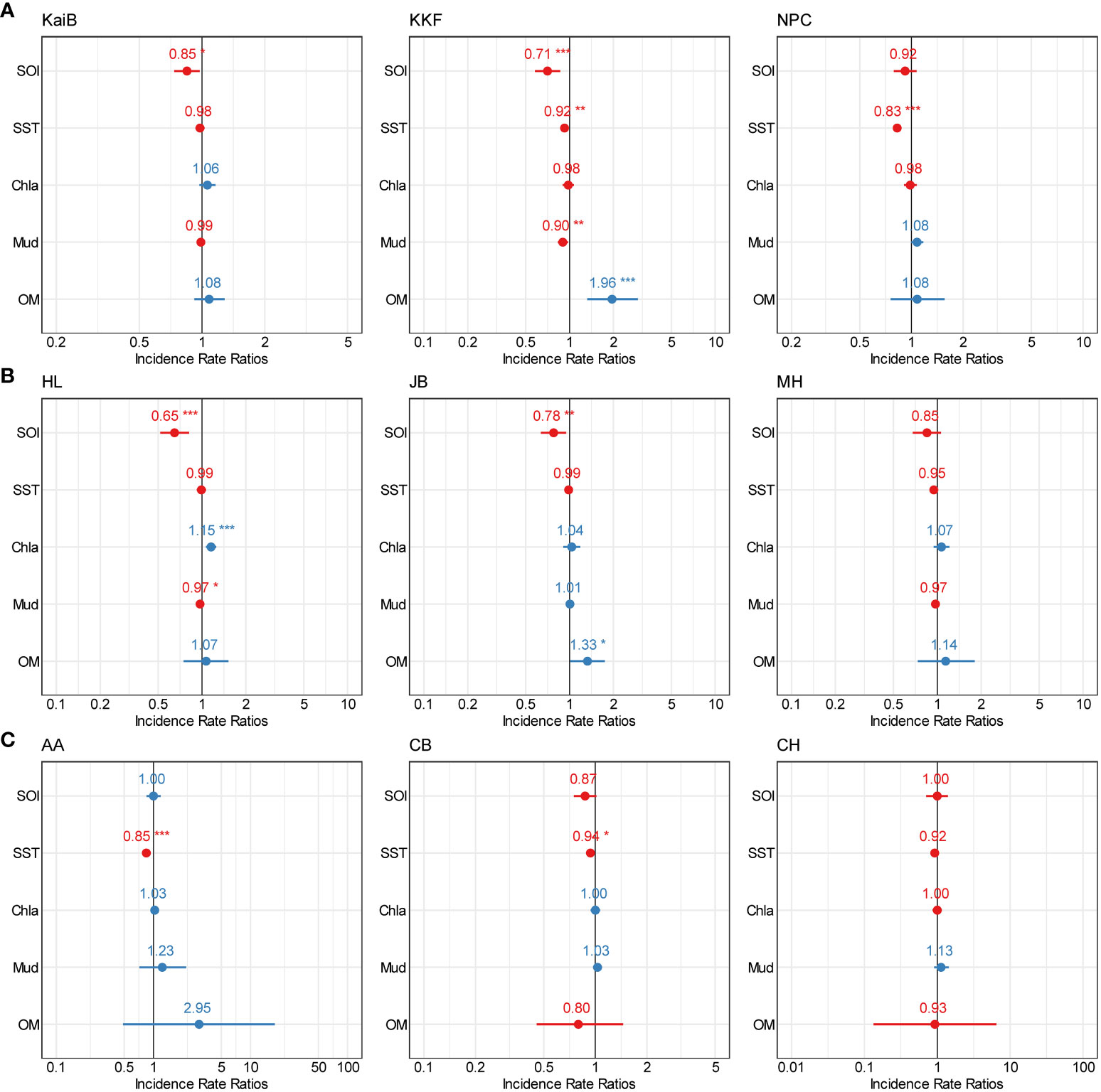
Figure 11 Forest plots summarising the outcomes from GLMs for each site (fine scale) showing point estimates (Incidence Rate Ratios) for relationships between multiple stressors and total crustacean abundance. (A) Kaipara estuary, (B) Mahurangi estuary, and (C) Manukau estuary. The colour indicates positive (blue) and negative (red) significant (*p=0.5; **p=0.01; ***p=0.001) interactions of the point estimates.

The abundance of crustaceans at Site HL was significatively influenced by SOI, Chl-a, and mud content. Crustacean abundance decreased with increasing SOI and mud content and increased with increasing Chl-a (Figure 11, Supplementary Figure 27, Supplementary Table 6). At the JB site, SOI and OM influenced crustacean abundance, driving decreases and increases in crustacean abundance, respectively (Figure 11, Supplementary Figure 28, Supplementary Table 6). AA and CB were influenced by SST, with crustacean abundance at both sites tending to decrease with increasing SST (Figure 11, Supplementary Figures 30, 31, Supplementary Table 6). At Sites MH and CH, crustacean abundance was unable to be predicted with any of the environmental variables available (Figure 11, Supplementary Figures 29–31, Supplementary Table 6).

4 Discussion

Climate change in combination with other environmental drives (e.g., nutrient and sediment inputs) are causing significant impacts on estuarine ecosystems (Kennish, 2021; Simeoni et al., 2023). The interaction of multiple environmental drivers, or multiple stressors, could exacerbate the deterioration of estuarine and coastal ecosystems, with negative consequences on living organisms, ecosystem functioning and services these important ecosystems provide (Kennish, 2021; Simeoni et al., 2023). The effects of multiple environmental drivers on estuarine ecosystems are occurring at accelerated rate, which challenges conservation and management efforts to improve the ecological health of these ecosystems. In this study, we analysed estuarine crustacean time-series data at three nested spatial scales—large (Auckland Region), medium (estuary within Auckland Region), and small (site within estuary)—to investigate the influence of multiple environmental variables related to freshwater, climate, and ocean drivers. There were trends over time in most of the environmental predictors, and our aim was to assess their potential effects on crustacean communities to improve prediction and our understanding of the interplay of multiple stressors. Our results showed that the abundance and richness of crustaceans, as well as the abundance of specific crustacean groups (i.e., Amphipoda, Decapoda, Cumacean, Tanaidacea), were influenced by unique combinations of environmental variables, resulting in scale dependent interactions.

Across all the spatial scales studied, combinations of the five predictor variables influenced estuarine crustaceans in at least one case. Our first study hypothesis, that crustaceans will respond to multiple stressors more often than to single stressors, appears to have been supported. However, the combinations of variables that were significant changed across scales, supporting our second hypothesis that the influence of environmental predictor variables would be scale dependent. The large-scale outcomes showed that crustacean abundance was influenced by SST and SOI (climatic and oceanic stressors). Temperature of the ocean has been described as a key factor shaping the structure of benthic communities (Tittensor et al., 2010; Clark et al., 2021). We identified that SST has increased at these estuarine sites by ~1°C over the last 20 years, and demonstrated that the abundance of crustaceans tended to decrease with increasing SST, which is consistent with other studies suggesting that the increase of ocean temperature could affect the morphology, life history, abundance, and distribution of benthic communities (Hewitt et al., 2016; Dvoretsky and Dvoretsky, 2020; Clark et al., 2021). SOI is an indicator of environmental variability that has the potential to affect other environmental drivers (e.g., wind and current speeds, air and water temperature, cloudiness and precipitation, storm frequency and intensity). Our results showed that SOI influenced both abundance and richness of estuarine crustaceans. With increased SOI (and generally warmer conditions during El Nino phases), the abundance and richness of crustaceans decreased. Coupled with evidencing of increasing SST through time, this suggests that climate and ocean warming may be an important stressor affecting the abundance and richness of key macroinvertebrate estuarine organisms in New Zealand (Hewitt et al., 2016; Clark et al., 2021).

Sediment muddiness was another stressor influencing both abundance and richness of estuarine crustaceans. Sediment mud content in estuarine receiving environments has increased with elevated sediment loadings associated with human-alterations of coastal catchments, an environmental change that has had major impacts on estuarine assemblages and ecosystem functions (Thrush et al., 2003b; Douglas et al., 2019). We observed that above a threshold of about 10-20% mud content, further increases in muddiness coincided with rapid decreases in crustacean abundance and richness. This threshold aligns with previous studies describing negative impacts on diversity and ecosystem functioning above 25% sediment mud content (Thrush et al., 2003a; Lohrer et al., 2004b; Ellis et al., 2017; Douglas et al., 2018; Douglas et al., 2019; Pardo et al., 2022), but perhaps suggests that crustaceans as a group are slightly more sensitive than macrofauna as a whole.

Excessive organic matter can be an environmental stressor in estuarine systems, often due to its effects on sediment oxygen demand and the potential for bottom water hypoxia/anoxia. Here, sediment OM was the only environmental variable that was positively associated with the abundance and richness of estuarine crustaceans. This is likely because of the value of organic material as a food resource for macrofauna, especially deposit feeders, when present at low to moderate levels. However, beyond a critical point (4-5%), excessive organic matter content can initiate the onset of eutrophication symptoms (Ellis et al., 2017) and negatively impact estuarine crustaceans.

Highly variable interactions between multiple environmental variables and estuarine crustaceans were identified at the medium (estuary) scale. However, there were isolated cases of consistency. For example, SST was inversely correlated with the abundance of crustaceans in both Kaipara and Manukau Harbours. Both of these harbours are large, west coast estuaries. The prevailing wind and ocean swell arrives in New Zealand from the southwest, so perhaps these climate and ocean forcings are stronger on New Zealand’s west coast relative to the east coast (Hewitt et al., 2016). Mahurangi Harbour (on the east coast) is smaller and more protected from prevailing southwesterlies, and may therefore be less responsive to the ocean and climate proxy variables that we used as environmental predictors.

Sediment muddiness and OM content had similar effects on the abundance and richness of crustaceans in Kaipara and Mahurangi Harbours. Freshwater inputs deliver fine sediments and organic matter to estuaries. Relative to Manukau Harbour, Kaipara and Mahurangi have more riverine influence, have larger catchment size to estuary size ratios, and are closer together geographically (which may translate to comparable rainfall totals). This may explain the relatively similar responses to increased muddiness and OM observed in Kaipara and Mahurangi Harbours.

Mud content had a relatively consistent negative effect on the abundance and richness of crustaceans across scales, though it was most apparent and detectable at the largest scales. With >10% bed sediment muddiness, decreases in the abundance and richness of crustaceans were readily apparent, consistent with analyses of other macrofauna datasets in New Zealand (Thrush et al., 2003b; Lohrer et al., 2004b; Ellis et al., 2017; Douglas et al., 2018).

In contrast to mud, OM had a generally positive influence on the abundance and richness of crustaceans across estuaries. This result was generally apparent at the large and medium spatial scales assessed. The final sediment variable used as an environmental predictor, Chl-a, was generally less influential. Significant effects of Chl-a at the estuary scale were only observed in Manukau Harbour. Manukau Harbour is a relatively turbid estuary and is large enough to have substantial wind-wave fetch. Both turbidity and wind-wave resuspension can limit microphytobenthos, a key food resource for the macroinvertebrate crustaceans investigated. This may explain why higher Chl-a resulted in higher crustacean abundance and richness in Manukau Harbour.

Results at the fine scale were highly site-specific, with crustacean responses generally influenced by fewer environmental variables and sometimes by only one predictor variable (or none). SST and SOI influenced crustacean abundance at the greatest number of individual sites (4/9 each). This outcome showed clear evidence of the potentially strong effects of climatic and oceanic drivers on estuarine communities (Hewitt et al., 2016; Clark et al., 2021). It is possible that the effects of the climate and ocean drivers are overriding the effects of sedimentary variables at the site scale (Thrush et al., 2008b; Hewitt et al., 2016; Ellis et al., 2017).

Our third study hypothesis was that different types of crustaceans (Amphipoda, Decapoda, Cumacea, Tanaidacea) would respond differently to multiple environmental predictors. We found some evidence of consistency in responses to multiple environmental drivers. For example, at the broader spatial scale, Amphipoda, Decapoda, and Tanaidacea were all influenced by OM, while Cumacea was influenced by stressors such as SST and sediment mud content. At the medium scale, results showed that Amphipoda and Cumacea were influenced by mud content, Decapoda was influenced by SST and OM, while Tanaidacea was not strongly influenced by any environmental variables at the medium scale. The mechanisms behind the differential responses of crustaceans to combinations of environmental variables are uncertain but could be linked to interactive effects and differences in the habitat requirements or tolerances of the four crustacean groups (Thrush et al., 2008b; Ellis et al., 2017; Dvoretsky and Dvoretsky, 2020; Clark et al., 2021).

It is important to highlight that the variance explained of estuarine crustaceans in our models was low (7%-51%). However, it is increasingly recognised that weak relationships can be ecologically meaningful and that, in empirical studies, models often account for ~10% of the variability (Thrush et al., 2008b; Hewitt et al., 2016). More importantly, our results suggest a pathway to shift from examination of single environmental drivers (or stressor) effects to multiple environmental stressor effects. We also provide evidence of different responses of estuarine crustaceans to multiple environmental drivers at multiple spatial scales, which have important implications for how we should consider ecological responses to climate change and other anthropogenic pressures. Our result could be used for reducing uncertainty of the interactions between crustacean communities and environmental drivers improving prediction of ecological change, which is critical for management efforts and created informed approaches to mitigate multiple environmental drivers impacts.

5 Conclusion

This study elucidated how environmental drivers associated with freshwater, climate and ocean forcings can influence estuarine crustacean time-series variation across different spatial scales. Scale dependent responses to multiple environmental predictors were found, with SST and SOI (ocean and climate variables, respectively) the most common drivers of the abundance and richness of estuarine crustaceans overall. Notably, negative responses to two known stressors—elevated sediment muddiness and increasing SST—were identified, with mud content negatively affecting crustacean communities at all the spatial scales. Our results provide further evidence that catchment sediment loading may be impacting the health and functioning of estuarine ecosystems, with effects potentially exacerbated by increasing SST associated with a warming climate. The observed interactions between estuarine crustaceans and climatic, oceanic, and freshwater drivers have important implications for predicting the ecological consequences of climate change in coastal ecosystems. We also highlight the need for management and conservations efforts to reduce sediment inputs and mitigate the effects of increasing temperatures to maintain the ecological health and functioning of estuarine ecosystems.

Data availability statement

The original contributions presented in the study are included in the article/Supplementary Material. Further inquiries can be directed to the corresponding author.

Ethics statement

The manuscript presents research on animals that do not require ethical approval for their study.

Author contributions

OL-G: Conceptualization, Data curation, Formal Analysis, Methodology, Visualization, Writing – original draft, Writing – review & editing. AL: Conceptualization, Funding acquisition, Writing – review & editing, Formal Analysis. ED: Methodology, Writing – review & editing. SH: Data curation, Methodology, Writing – review & editing. KC: Data curation, Methodology, Writing – review & editing. BG: Data curation, Methodology, Writing – review & editing.

Funding

The author(s) declare financial support was received for the research, authorship, and/or publication of this article. Analysis was funded by NIWA Coasts & Oceans Strategic Science Investment Funding with additional support from Ministry for the Environment. Auckland Council funded data gathering (field work and sample collection/processing) at all of the study sites.

Acknowledgments

We would like to thank the many NIWA Marine Ecology technicians who have collected, processed and quality-checked estuarine macrofauna samples under contract from Auckland Council for decades. We thank the funders of data collection and analysis (Auckland Council, MfE, NIWA) and Auckland Council for permission to use the data.

Conflict of interest

The authors declare that the research was conducted in the absence of any commercial or financial relationships that could be construed as a potential conflict of interest.

Publisher’s note

All claims expressed in this article are solely those of the authors and do not necessarily represent those of their affiliated organizations, or those of the publisher, the editors and the reviewers. Any product that may be evaluated in this article, or claim that may be made by its manufacturer, is not guaranteed or endorsed by the publisher.

Supplementary material

The Supplementary Material for this article can be found online at: https://www.frontiersin.org/articles/10.3389/fmars.2023.1292849/full#supplementary-material

References

Agusto L. E., Qin G., Thibodeau B., Tang J., Zhang J., Zhou J., et al. (2022). Fiddling with the blue carbon: Fiddler crab burrows enhance CO2 and CH4 efflux in saltmarsh. Ecol. Indic. 144 (109538). doi: 10.1016/j.ecolind.2022.109538

CrossRef Full Text | Google Scholar

Barbier E. B., Hacker S. D., Kennedy C., Koch E. W., Stier A. C., Silliman B. R. (2011). The value of estuarine and coastal ecosystem services. Ecol. Monogr. 81 (2), 169–193. doi: 10.1890/10-1510.1

CrossRef Full Text | Google Scholar

Bastakoti U., Bourgeois C., Marchand C., Alfaro A. C. (2019). Urban-rural gradients in the distribution of trace metals in sediments within temperate mangroves (New Zealand). Mar. pollut. Bull. 149 (110614). doi: 10.1016/j.marpolbul.2019.110614

CrossRef Full Text | Google Scholar

Behrens E., Rickard G., Rosier S., Williams J., Morgenstern O., Stone D. (2022). Projections of future marine heatwaves for the oceans around New Zealand using New Zealand’s earth system model. Front. Climate 4. doi: 10.3389/fclim.2022.798287

CrossRef Full Text | Google Scholar

Borja A., Franco J., Pérez V. (2000). A marine biotic index to establish the ecological quality of soft-bottom benthos with European estuarine and coastal environments. Mar. pollut. Bull. 40, 1100–1114. doi: 10.1016/S0025-326X(00)00061-8

CrossRef Full Text | Google Scholar

Bui T. H. H., Lee S. Y. (2014). Does “you are what you eat” apply to mangrove grapsid crabs? PloS One 9. doi: 10.1371/journal.pone.0089074

CrossRef Full Text | Google Scholar

Bulmer R. H., Kelly S., Jeffs A. G. (2016). Light requirements of the seagrass, Zostera muelleri, determined by observations at the maximum depth limit in a temperate estuary, New Zealand. New Z. J. Mar. Freshw. Res. 50 (2), 183–194. doi: 10.1080/00288330.2015.1120759

CrossRef Full Text | Google Scholar

Carrier-Belleau C., Drolet D., McKindsey C., Archambault P. (2021). Environmental stressors, complex interactions and marine benthic communities’ responses. Sci. Rep. 11. doi: 10.1038/s41598-021-83533-1

PubMed Abstract | CrossRef Full Text | Google Scholar

Chapman P. M. (2016). Assessing and managing stressors in a changing marine environment. Mar. pollut. Bull. 124 (2), 587–590. doi: 10.1016/j.marpolbul.2016.10.039

PubMed Abstract | CrossRef Full Text | Google Scholar

Clark D. E., Stephenson F., Hewitt J. E., Ellis J. I., Zaiko A., Berthelsen A., et al. (2021). Influence of land-derived stressors and environmental variability on compositional turnover and diversity of estuarine benthic communities. Mar. Ecol. Prog. Ser. 666, 1–18. doi: 10.3354/meps13714

CrossRef Full Text | Google Scholar

Cloern J. E., Abreu P. C., Carstensen J., Chauvaud L., Elmgren R., Grall J., et al. (2016). Human activities and climate variability drive fast-paced change across the world's estuarine–coastal ecosystems. Globlal Change Biol. 22, 513–529. doi: 10.1111/gcb.13059

CrossRef Full Text | Google Scholar

Dauvin J. C., Desroy N., Janson A. L., Vallet C., Duhamel S. (2006). Recent changes in estuarine benthic and suprabenthic communities resulting from the development of harbour infrastructure. Mar. pollut. Bull. 53, 80–90. doi: 10.1016/j.marpolbul.2005.09.020

PubMed Abstract | CrossRef Full Text | Google Scholar

De Grave S., Decock W., Dekeyzer S., Davie P. J. F., Fransen C. H. J. M., Boyko C. B., et al. (2023). Benchmarking global biodiversity of decapod crustaceans (Crustacea: Decapoda). J. Crustacean Biol. 43 (3), 1–9. doi: 10.1093/jcbiol/ruad042

CrossRef Full Text | Google Scholar

Douglas E. J., Lohrer A. M., Pilditch C. A. (2019). Biodiversity breakpoints along stress gradients in estuaries and associated shifts in ecosystem interactions. Sci. Rep. 9 (1), 17567. doi: 10.1038/s41598-019-54192-0

PubMed Abstract | CrossRef Full Text | Google Scholar

Douglas E. J., Pilditch C. A., Kraan C., Schipper L. A., Lohrer A. M., Thrush S. F. (2017). Macrofaunal functional diversity provides resilience to nutrient enrichment in coastal sediments. Ecosystems 20 (7), 1324–1336. doi: 10.1007/s10021-017-0113-4

CrossRef Full Text | Google Scholar

Douglas E. J., Pilditch C. A., Lohrer A. M., Savage C., Schipper L. A., Thrush S. F. (2018). Sedimentary environment influences ecosystem response to nutrient enrichment. Estuaries Coasts 41, 1994–2008. doi: 10.1007/s12237-018-0416-5

CrossRef Full Text | Google Scholar

Drylie T. P. (2021). Marine ecology state and trends in Tāmaki Makaurau / Auckland to 2019. State of the environment reporting (Auckland, New Zealand: Auckland Council technical report). TR2021/09.

Google Scholar

Dvoretsky A. G., Dvoretsky V. G. (2020). Effects of environmental factors on the abundance, biomass, and individual weight of juvenile red king crabs in the barents sea. Front. Mar. Sci. 7 (726). doi: 10.3389/fmars.2020.00726

CrossRef Full Text | Google Scholar

Ellis J., Nicholls P., Craggs R., Hofstra D., Hewitt J. (2004). Effects of terrigenous sedimentation on mangrove physiology and associated macrobenthic communities. Mar. Ecol. Prog. Ser. 270, 714–782. doi: 10.3354/meps270071

CrossRef Full Text | Google Scholar

Ellis J. I., Clark D., Atalah J., Jiang W., Taiapa C., Patterson M., et al. (2017). Multiple stressor effects on marine infauna: responses of estuarine taxa and functional traits to sedimentation, nutrient and metal loading. Sci. Rep. 7 (12013). doi: 10.1038/s41598-017-12323-5

PubMed Abstract | CrossRef Full Text | Google Scholar

Fanjul E., Escapa M., Montemayor D., Addino M., Alvarez M. F., Grela M. A., et al. (2015). Effect of crab bioturbation on organic matter processing in South West Atlantic intertidal sediments. J. Sea Res. 95, 206–216. doi: 10.1016/j.seares.2014.05.005

CrossRef Full Text | Google Scholar

Fox J., Weisberg S. (2019). “An R Companion to Applied Regression,”, 3rd ed. (Thousand Oaks CA: Sage).

Google Scholar

Gibbs M., Funnell G., Pickmere S., Norkko A., Hewitt J. (2005). Benthic nutrient fluxes along an estuarine gradient: influence of the pinnid bivalve Atrina zelandica in summer. Mar. Ecol. Prog. Ser. 288, 151–164. doi: 10.3354/meps288151

CrossRef Full Text | Google Scholar

Gorman R. M., Neilson C. G. (1999). Modelling shallow water wave generation and transformation in an intertidal estuary. Coast. Eng. 36 (3), 197–217. doi: 10.1016/S0378-3839(99)00006-X

CrossRef Full Text | Google Scholar

Goulding T., Sousa P. M., Silva G., Medeiros J. P., Carvalho F., Metelo I., et al. (2021). Shifts in estuarine macroinvertebrate communities associated with water quality and climate change. Front. Mar. Sci. 8. doi: 10.3389/fmars.2021.698576

CrossRef Full Text | Google Scholar

Green M. O., Bell R. G., Dolphin T. J., Swales A. (2000). Silt and sand transport in a deep tidal channel of a large estuary (Manukau Harbour, New Zealand). Mar. Geol. 163, 217–240. doi: 10.1016/S0025-3227(99)00102-4

CrossRef Full Text | Google Scholar

Greenfield B. L., Hailes S., MacLean F., Peart R., Read G. B., Marshall B., et al. (2023). “Protocol for the Identification of Benthic Estuarine and Marine Macroinvertebrates: A guide for parataxonomists,” in C-SIG Coastal Taxonomic Resource Tool. Wellington, New Zealand. vol. 40.

Google Scholar

Gunderson A. R., Armstrong E. J., Stillman J. H. (2016). Multiple stressors in a changing world: the need for an improved perspective on physiological responses to the dynamic marine environment. Annu. Rev. Mar. Sci. 8, 357–378. doi: 10.1146/annurev-marine-122414-033953

CrossRef Full Text | Google Scholar

Heath R. A. (1975). Stability of some New Zealand coastal inlets. New Z. J. Mar. Freshw. Res. 9, 449–457. doi: 10.1080/00288330.1975.9515580

CrossRef Full Text | Google Scholar

Hewitt J. E., Ellis J. I., Thrush S. F. (2016). Multiple stressors, nonlinear effects and the implications of climate change impacts on marine coastal ecosystems. Global Change Biol. 22, 2665–2675. doi: 10.1111/gcb.13176

CrossRef Full Text | Google Scholar

Hewitt J. E., Hailes. S. F., Greenfield B. L. (2014). Protocol for processing, identification and quality assurance of New Zealand marine benthic invertebrate samples. Prepared Northland Regional Council 36, 1–36.

Google Scholar

Hicks M., Semadeni-Davies A., Haddadchi A., Shankar U., Plew D. (2019). Updated sediment load estimator for New Zealand. Prepared for the Ministry for the Environment. Hamilton, New Zealand. 190, NIWA Client Report 2018341CH.

Google Scholar

Hillman J. R., Lundquist C. J., O’Meara T. A., Thrush S. F. (2020). Loss of large animals differentially influences nutrient fluxes across a heterogeneous marine intertidal soft-sediment ecosystem. Ecosystems 24 (2), 272–283. doi: 10.1007/s10021-020-00517-4

CrossRef Full Text | Google Scholar

Hunt S. (2019). Summary of historic sedimentation measurements in the Waikato region and formulation of a historic baseline sedimentation rates, WRC Tech. Report 2019/08.

Google Scholar

Kassambara A. (2020) ggpubr: 'ggplot2' Based Publication Ready Plots. Available at: https://CRAN.R-project.org/package=ggpubr.

Google Scholar

Kennish M. J. (2021). Drivers of change in estuarine and coastal marine environments: an overview. Open J. Ecol. 11 (3), 224–239. doi: 10.4236/oje.2021.113017

CrossRef Full Text | Google Scholar

Kristensen E., Penha-Lopes G., Delefosse M., Valdemarsen T., Quintana C. O., Banta G. T. (2012). What is bioturbation? The need for a precise definition for fauna in aquatic sciences. Mar. Ecol. Prog. Ser. 446, 285–302. doi: 10.3354/meps09506

CrossRef Full Text | Google Scholar

Lam-Gordillo O., Baring R., Dittmann S. (2021). Taxonomic and functional patterns of benthic communities in Southern temperate tidal flats. Front. Mar. Sci. 8. doi: 10.3389/fmars.2021.723749

CrossRef Full Text | Google Scholar

Lam-Gordillo O., Huang J., Barcelo A., Kent J., Mosley L. M., Welsh D. T., et al. (2022a). Restoration of benthic macrofauna promotes biogeochemical remediation of hostile sediments; An in situ transplantation experiment in a eutrophic estuarine-hypersaline lagoon system. Sci. Total Environ. 833, 155201. doi: 10.1016/j.scitotenv.2022.155201

PubMed Abstract | CrossRef Full Text | Google Scholar

Lam-Gordillo O., Mosley L. M., Simpson S. L., Welsh D. T., Dittmann S. (2022b). Loss of benthic macrofauna functional traits correlates with changes in sediment biogeochemistry along an extreme salinity gradient in the Coorong lagoon, Australia. Mar. pollut. Bull. 174, 113202. doi: 10.1016/j.marpolbul.2021.113202

PubMed Abstract | CrossRef Full Text | Google Scholar

Lohrer A. M., Hewitt J. E., Thrush S. F. (2006). Assessing far-field effects of terrigenous sediment loading in the coastal marine environment. Mar. Ecol. Prog. Ser. 315), 13–18. doi: 10.3354/meps315013

CrossRef Full Text | Google Scholar

Lohrer A., Thrush S., Gibbs M. (2004a). Bioturbators enhance ecosystem function through complex biogeochemical interactions. Nature 431, 1092–1095. doi: 10.1038/nature03042

PubMed Abstract | CrossRef Full Text | Google Scholar

Lohrer A. M., Thrush S. F., Hewitt J. E., Berkenbusch K., Ahrens M., Cummings V. J. (2004b). Terrestrially derived sediment: response of marine macrobenthic communities to thin terrigenous deposits. Mar. Ecol. Prog. Ser. 273), 121–138. doi: 10.3354/meps273121

CrossRef Full Text | Google Scholar

Lohrer A. M., Townsend M., Rodil I. F., Hewitt J. E., Thrush S. F. (2012). Detecting shifts in ecosystem functioning: the decoupling of fundamental relationships with increased pollutant stress on sandflats. Mar. pollut. Bull. 64 (12), 2761–2769. doi: 10.1016/j.marpolbul.2012.09.012

PubMed Abstract | CrossRef Full Text | Google Scholar

Lüdecke D. (2023). sjPlot: Data Visualization for Statistics in Social Science. Available at: https://strengejacke.github.io/sjPlot/.

Google Scholar

Malone T. C., Newton A. (2020). The globalization of cultural eutrophication in the coastal ocean: causes and consequences. Front. Mar. Sci. 7 (670). doi: 10.3389/fmars.2020.00670

CrossRef Full Text | Google Scholar

Medina-Contreras D., Arenas F., Cantera-Kintz J., Sánchez A., Lázarus J.-F. (2022). Carbon sources supporting macrobenthic crustaceans in tropical eastern pacific mangroves. Food Webs 30, e00219. doi: 10.1016/j.fooweb.2022.e00219

CrossRef Full Text | Google Scholar

Needham H. R., Pilditch C. A., Lohrer A. M., Thrush S. F. (2011). Context-specific bioturbation mediates changes to ecosystem functioning. Ecosystems 14 (7), 1096–1109. doi: 10.1007/s10021-011-9468-0

CrossRef Full Text | Google Scholar

Needham H. R., Pilditch C. A., Lohrer A. M., Thrush S. F. (2013). Density and habitat dependent effects of crab burrows on sediment erodibility. J. Sea Res. 76, 94–104. doi: 10.1016/j.seares.2012.12.004

CrossRef Full Text | Google Scholar

Nozarpour R., Shojaei M. G., Naderloo R., Nasi F. (2023). Crustaceans functional diversity in mangroves and adjacent mudflats of the Persian Gulf and Gulf of Oman. Mar. Environ. Res. 186, 105919. doi: 10.1016/j.marenvres.2023.105919

PubMed Abstract | CrossRef Full Text | Google Scholar

Oldman J. W., Black K. P., Swales A., Stroud M. J. (2009). Prediction of annual average sedimentation rates in an estuary using numerical models with verification against core data – Mahurangi Estuary, New Zealand. Estuarine Coast. Shelf Sci. 84 (4), 483–492. doi: 10.1016/j.ecss.2009.05.032

CrossRef Full Text | Google Scholar

Oliver E. C. J., Benthuysen J. A., Darmaraki S., Donat M. G., Hobday A. J., Holbrook N. J., et al. (2021). Marine heatwaves. 13 (1), 313–342. doi: 10.1146/annurev-marine-032720-095144

CrossRef Full Text | Google Scholar

Oliver E. C. J., Donat M. G., Burrows M. T., Moore P. J., Smale D. A., Alexander L. V., et al. (2018). Longer and more frequent marine heatwaves over the past century. Nat. Commun. 9, 1324. doi: 10.1038/s41467-018-03732-9

CrossRef Full Text | Google Scholar

O’Meara T. A., Hewitt J. E., Thrush S. F., Douglas E. J., Lohrer A. M. (2020). Denitrification and the role of macrofauna across estuarine gradients in nutrient and sediment loading. Estuaries Coasts 43 (6), 1394–1405. doi: 10.1007/s12237-020-00728-x

CrossRef Full Text | Google Scholar

Pardo J. C. F., Poste A. E., Frigstad H., Quintana C. O., Trannum H. C. (2022). The interplay between terrestrial organic matter and benthic macrofauna: Framework, synthesis, and perspectives. Ecosphere 14, e4492. doi: 10.1002/ecs2.4492

CrossRef Full Text | Google Scholar

Pine M. K., Radford C. A., Jeffs A. G. (2015). Eavesdropping on the Kaipara Harbour: characterising underwater soundscapes within a seagrass bed and a subtidal mudflat. New Z. J. Mar. Freshw. Res. 49 (2), 247–258. doi: 10.1080/00288330.2015.1009916

CrossRef Full Text | Google Scholar

R-Core-Team (2022). R: A language and environment for statistical computing (Vienna, Austria: R Foundation for Statistical Computing). Available at: https://www.R-project.org/.

Google Scholar

Robertson B. M., Gillespie P. A., Asher R. A., Frisk S., Keeley N. B., Hopkins G. A., et al. (2002). Estuarine environmental assessment and monitoring: A national protocol. Prepared support. Councils Ministry Environ. Sustain. Manage. Fund. 5096, 93–159.

Google Scholar

Rullens V., Lohrer A. M., Townsend M., Pilditch C. A. (2019). Ecological mechanisms underpinning ecosystem service bundles in marine environments – A case study for shellfish. Front. Mar. Sci. 6. doi: 10.3389/fmars.2019.00409

CrossRef Full Text | Google Scholar

Sánchez-Moyano J. E., García-Asencio I. (2010). Crustacean assemblages in a polluted estuary from South-Western Spain. Mar. pollut. Bull. 60, 1890–1897. doi: 10.1016/j.marpolbul.2010.07.016

PubMed Abstract | CrossRef Full Text | Google Scholar

Sartory D. P. (1982). Spectrophotometric Analysis of Chlorophyll a in Freshwater Phytoplankton. . Report No. TR 115 (Pretoria: Hydrological Research Institute, Department of Environment Affairs), 163.

Google Scholar

Seitzinger S. P. (1988). Denitrification in freshwater and coastal marine ecosystems: Ecological and geochemical significance. Limnol. Oceanogr. 33 (4), 702–724. doi: 10.4319/lo.1988.33.4_part_2.0702

CrossRef Full Text | Google Scholar

Simeoni C., Furlan E., Pham H. V., Critto A., de Juan S., Trégarot E., et al. (2023). Evaluating the combined effect of climate and anthropogenic stressors on marine coastal ecosystems: Insights from a systematic review of cumulative impact assessment approaches. Sci. Total Environ. 861, 160687. doi: 10.1016/j.scitotenv.2022.160687

PubMed Abstract | CrossRef Full Text | Google Scholar

Thrush S. F., Halliday J., Hewitt J. E., Lohrer A. M. (2008a). The effects of habitat loss, fragmentation, and community homogenization on resilience in estuaries. Ecol. Appl. 18 (1), 12–21. doi: 10.1890/07-0436.1

PubMed Abstract | CrossRef Full Text | Google Scholar

Thrush S. F., Hewitt J. E., Cummings V. J., Ellis J. I., Hatton C., Lohrer A., et al. (2004). Muddy waters: elevating sediment input to coastal and estuarine habitats. Front. Ecol. Environ. 2 (6), 299–306. doi: 10.1890/1540-9295(2004)002[0299:MWESIT]2.0.CO;2

CrossRef Full Text | Google Scholar

Thrush S. F., Hewitt J. E., Gladstone-Gallagher R. V., Savage C., Lundquist C., O'Meara T., et al. (2021). Cumulative stressors reduce the self-regulating capacity of coastal ecosystems. Ecol. Appl. 31 (1), e02223. doi: 10.1002/eap.2223

PubMed Abstract | CrossRef Full Text | Google Scholar

Thrush S. F., Hewitt J. E., Hickey C. W., Kelly S. (2008b). Multiple stressor effects identified from species abundance distributions: Interactions between urban contaminants and species habitat relationships. J. Exp. Mar. Biol. Ecol. 366, 160–168. doi: 10.1016/j.jembe.2008.07.020

CrossRef Full Text | Google Scholar

Thrush S. F., Hewitt J. E., Kraan C., Lohrer A. M., Pilditch C. A., Douglas E. (2017). Changes in the location of biodiversity-ecosystem function hot spots across the seafloor landscape with increasing sediment nutrient loading. Proc. Biol. Sci. 284 (1852). doi: 10.1098/rspb.2016.2861

CrossRef Full Text | Google Scholar

Thrush S. F., Hewitt J. E., Norkko A., Cummings V. J., Funnell G. A. (2003a). Macrobenthic recovery processes following catastrophic sedimentation on estuarine sandflats. Ecol. Appl. 13, 1433–1455. doi: 10.1890/02-5198

CrossRef Full Text | Google Scholar

Thrush S. F., Hewitt J. E., Norkko A., Nicholls P. E., Funnell G. A., Ellis J. I. (2003b). Habitat change in estuaries: predicting broad-scale responses of intertidal macrofauna to sediment mud content. Mar. Ecol. Prog. Ser. 263, 113–125. doi: 10.3354/meps263101

CrossRef Full Text | Google Scholar

Thrush S. F., Townsend M., Hewitt J. E., Davies K., Lohrer A. M., Lundquist C., et al. (2013). The many uses and values of estuarine ecosystems. Ecosystem services in New Zealand–conditions and trends (Lincoln, New Zealand: Manaaki Whenua Press), 226–237.

Google Scholar

Tittensor D. P., Mora C., Jetz W., Lotze H. K., Ricard D., Berghe E. V., et al. (2010). Global patterns and predictors of marine biodiversity across taxa. Nature 466, 1098–1101. doi: 10.1038/nature09329

PubMed Abstract | CrossRef Full Text | Google Scholar

Venables W. N., Ripley B. D. (2002). Modern Applied Statistics with S-Plus. 4th ed. (New York: Springer), ISBN: ISBN 0-387-95457-0.

Google Scholar

Villnäs A., Janas U., Josefson A. B., Kendzierska H., Nygård H., Norkko J., et al. (2019). Changes in macrofaunal biological traits across estuarine gradients: implications for the coastal nutrient filter. Mar. Ecol. Prog. Ser. 622, 31–48. doi: 10.3354/meps13008

CrossRef Full Text | Google Scholar

Welsh D. T. (2003). It’s a dirty job but someone has to do it: the role of marine benthic macrofauna in organic matter turnover and nutrient recycling to the water column. J. Chem. Ecol. 19, 321–324. doi: 10.1080/0275754031000155474

CrossRef Full Text | Google Scholar

Xu T., Newman M., Capotondi A., Stevenson S., Di Lorenzo E., Alexander M. A. (2022). An increase in marine heatwaves without significant changes in surface ocean temperature variability. Nat. Commun. 13 (7396). doi: 10.1038/s41467-022-34934-x

CrossRef Full Text | Google Scholar

Zetina-Rejon M. J., Arreguín-Sanchez F., Chavez E. A. (2003). Trophic structure and flows of energy in the Huizache-Caimanero lagoon complex on the Pacific coast of Mexico. Estuarine Coast. Shelf Sci. 57, 803–815. doi: 10.1016/S0272-7714(02)00410-9

CrossRef Full Text | Google Scholar