Modelling of fluid mud flow based on a three-dimensional hydrodynamic model : incorporating a 3D rheological model

Modeling fluid mud in estuaries and coastal areas is a complicated task due to its non-Newtonian characteristics. A continuous modeling approach was adopted to investigate the laminar flow of fluid mud, with a three-dimensional (3D) form of the Herschel–Bulkley rheological model introduced into the finite volume coastal ocean model (FVCOM) to calculate the apparent viscosity of fluid mud. The model was validated against two flume experiments for the laminar flow of fluid mud. The results showed that the developed model was capable of accurately reflecting the continuous distribution of velocity and density from the near-bottom to the upper water column. Based on the validated model, the difference between the 3D rheological model and a 1DV rheological model on the simulation results was assessed. The study found the results of the 1DV model and the 3D model show obvious differences. This illustrates the significant effect of apparent viscosity in horizontal direction taken into account by the 3D rheological model.

1 Introduction

Fluid mud is a highly concentrated suspended layer of cohesive sediment (Kirby, 1988), usually in the density range of 1080–1200 kg/m³; it is non-Newtonian and can form gravity currents along slopes or move horizontally in response to waves and tidal currents (McAnally et al., 2007a). Fluid mud has been observed in many estuaries and coastal areas around the world, such as the Amazon shelf, the Hudson estuary, the Mississippi River delta, the Changjiang River estuary, and the Weser estuary (Trowbridge and Kineke, 1994; Kineke and Sternberg, 1995; Kineke et al., 1996; Traykovski et al., 2004; Reide Corbett et al., 2007; Shi, 2010; Becker et al., 2013; Azhikodan and Yokoyama, 2018; James et al., 2020; Wu et al., 2022). This fluid mud, which sometimes even accumulates to several meters thick, can change navigable depths (Wurpts, 2005) and present critical management problems (McAnally et al., 2007a; McAnally et al., 2007b). Therefore, it is important to understand the dynamics of fluid mud motion in coastal and estuarine areas through experimental and field measurements or numerical modeling.

As for the numerical simulation of fluid mud motion in a large field area, usually two- or three-dimensional shallow water hydrodynamic models considering non-Newtonian properties of fluid mud have been applied. For most of these numerical models, the fluid mud was defined as a separate layer and coupled with the upper hydrodynamic model. For example, Odd and Cooper (1989) developed a two-layer model to simulate the fluid mud movement in the Severn River, with a depth averaged 2D model of the water column overlaying a fluid mud layer. In their model, the fluid mud layer was defined as a Bingham fluid with uniform density, and the yield stress and friction of the bottom bed were introduced into the momentum equation to describe the non-Newtonian properties of the fluid mud. Roberts (1993) simplified the equation of Odd and Cooper (1989) by removing the yield stress in the momentum equation and reflecting the non-Newtonian properties only through the bottom shear stress. Based on the Odd and Cooper (1989) model, Wang and Winterwerp (1992) developed a fluid mud model that considers the interaction between the suspension layer and fluid mud layer. This model later became the fluid mud module of the Delft3D model (Deltares, 2021). Similar approaches have been implemented in other models, such as TELEMAC-3D and the FVCOM (Normant, 2000; Yang et al., 2015). These horizontal two-dimensional numerical models are computationally economical and have been widely used for accounting for fluid mud flows in practical investigations (Van Haaren, 1995; Chung, 1998; Winterwerp et al., 2002; Wang et al., 2008; Ge et al., 2020). However, these models cannot simulate the full interaction between the water above and the fluid mud layer (of uniform density), with semiempirical exchange formulations between them for entrainment and settling. Furthermore, the models assume a strong discontinuity at the water/fluid mud interface and no vertical velocity gradient within the fluid mud, and they fail to reproduce the actual fluid mud dynamics (Le Hir et al., 2000). Knoch and Malcherek (2011) developed an isopycnal numerical model to simulate fluid mud, which divides the fluid mud layer vertically into a multilayer system, each layer with an identical density, and introduces rheological models to calculate the apparent viscosity of the fluid mud, thus reproducing the shear thinning properties of the fluid mud. This model is able to represent stratified flow conditions but lacks vertical mixing processes (Schmidt and Malcherek, 2021).

In contrast to the method of defining fluid mud as a separate layer, Le Hir et al. (2000) presented a continuous modeling approach on a vertical 2D model, considering water layers and fluid mud layers as a whole and solving mass conservation and momentum equations over an entire column, to reproduce the continuous transition from the fluid mud layer to the suspension layer. The total viscosity is described as the sum of the eddy diffusion viscosity and the apparent viscosity calculated by the rheological model. This method provides a continuous transition between water and fluid mud, and the vertical mixing of fluid mud can be considered. Subsequently, Le Hir and Cayocca (2002) extended this continuous modeling approach into a 3D model and simulated the gravity current of fluid mud on a slope. Guan et al. (2005) adopted this continuous concept into the Princeton ocean model (POM) to investigate the fluid mud process in the Jiaojiang estuary in China. Recently, Oberrecht (2021) applied this continuous modeling approach to the Delft3D model and simulated fluid mud processes in the Ems estuary. Chmiel et al. (2021) developed a vertical one-dimensional model by modifying the k-ω turbulence model (Wilcox, 1988) to reproduce the vertical mixing from the fluid mud layer to the water layer, and Schmidt and Malcherek (2021) applied the model to the Ems estuary and obtained satisfactory simulation results.

In summary, the continuous modeling approach based on 3D shallow water equations is gaining more extensive application due to its capability of simulating sediment suspensions and fluid mud motion interactively. Nevertheless, all previous numerical models with the continuous modeling approach adopted the apparent viscosity from the one-dimensional rheological model (1DV model), which solely depends on the vertical gradient of velocities, and the effect of velocity shear in horizontal directions is ignored. Theoretically, in 3D models, the apparent viscosity should take into account the three-dimensional velocity shear, which means that the horizontal velocity shear should be considered in the calculation of viscosity, while the 1DV model only considers the vertical velocity shear. A 3D rheology model will address this limitation.

The objective of this paper is to develop a numerical model for fluid mud motion, by introducing the apparent viscosity through a 3D Herschel–Bulkley rheological model, incorporating three-dimensional shear effects allows for the representation of fluid mud movement. The sections are arranged as follows. In Section 2, the numerical model is established, including the introduction of the apparent viscosity to the finite volume community ocean model (FVCOM), the formulation of the 3D form of the Herschel–Bulkley rheological model in a terrain-following coordinate system that was used to calculate the apparent viscosity, and the numerical discretization of the developed model. In Section 3, the developed model is validated against experimental data on the laminar flow of fluid mud from van Kessel and Kranenburg (1996) and Chowdhury and Testik (2012). In Section 4, an ideal case is set up, and the simulation results of the apparent viscosities from the 3D Herschel–Bulkley rheological model and its 1DV form are compared and assessed. In Section 5, a summary is given, and further considerations are suggested.

2 Numerical model for the water–fluid mud system

2.1 FVCOM model

The numerical model was based on FVCOM. The FVCOM model is a 3D ocean model based on unstructured grids and finite volume methods developed by Chen et al. (2003). The model is discretized using a triangular grid in the horizontal direction and a terrain-following coordinate system in the vertical direction. The governing equations of continuity equations (Equation 1, vertically integrated), momentum conservation with the Boussinesq approximation (Equations 2–4), sediment transport (Equation 5) and density (Equation 6) in the terrain-following coordinate system are as follows:

$\begin{array}{ll}\frac{\partial \zeta }{\partial t}+\frac{\partial (\overline{u}D)}{\partial x}+\frac{\partial (\overline{v}D)}{\partial y}=0& (1)\end{array}$

$\begin{array}{ll}\begin{array}{l}\frac{\partial uD}{\partial t}+\frac{\partial u^{2}D}{\partial x}+\frac{\partial uvD}{\partial y}+\frac{\partial u\omega }{\partial \sigma }-fvD=-ɡD\frac{\partial \zeta }{\partial x}-\frac{ɡD}{{\rho }_0}[\frac{\partial }{\partial x}(D{\displaystyle {\int }_{\sigma }^0\rho d{\sigma }^{\prime }})+\sigma \rho \frac{\partial D}{\partial x}]\\ +\frac{1}{D}\frac{\partial }{\partial \sigma }(K_m\frac{\partial u}{\partial \sigma })+\frac{\partial }{\partial x}[2A_{m}H\frac{\partial u}{\partial x}]+\frac{\partial }{\partial y}[A_{m}H(\frac{\partial u}{\partial y}+\frac{\partial v}{\partial x})]\end{array}& (2)\end{array}$

$\begin{array}{ll}\begin{array}{l}\frac{\partial vD}{\partial y}+\frac{\partial uvD}{\partial x}+\frac{\partial v^{2}D}{\partial y}+\frac{\partial v\omega }{\partial \sigma }+fuD=-ɡD\frac{\partial \zeta }{\partial y}-\frac{ɡD}{{\rho }_0}[\frac{\partial }{\partial y}(D{\displaystyle {\int }_{\sigma }^0\rho d{\sigma }^{\prime }})+\sigma \rho \frac{\partial D}{\partial y}]\\ +\frac{1}{D}\frac{\partial }{\partial \sigma }(K_m\frac{\partial v}{\partial \sigma })+\frac{\partial }{\partial x}[A_{m}H(\frac{\partial }{\partial x}+\frac{\partial v}{\partial x})]+\frac{\partial }{\partial y}[2A_{m}H\frac{\partial v}{\partial y}]\end{array}& (3)\end{array}$

$\begin{array}{ll}\frac{\partial P}{\partial \sigma }=-D\rho ɡ& (4)\end{array}$

$\begin{array}{ll}\frac{\partial C_{s}D}{\partial t}+\frac{\partial C_{s}uD}{\partial x}+\frac{\partial C_{s}vD}{\partial y}+\frac{\partial C_s(\omega -{\omega }_i)}{\partial \sigma }=\frac{1}{D}\frac{\partial }{\partial \sigma }(K_h\frac{\partial C_s}{\partial \sigma })+D{F}_c& (5)\end{array}$

$\begin{array}{ll}\rho ={\rho }_0+C_s(1-{\rho }_0/{\rho }_s)& (6)\end{array}$

where x, y, and σ are the directions of the east, north and vertical axes of the terrain-following coordinate system. Figure 1 is a schematic diagram illustrating the original vertical space and discretization in the σ coordinate system, where k represents the layer number. u, v, and ω are the velocities in the x, y, and σ directions (m/s). $\overline{u}$ and $\overline{v}$ are the velocities vertically integrated from u and v. ω_i is the settling velocity of sediment (m/s). t is the time (s). D is the total water depth (m), which is equal to the sum of the static water depth h (m) and the water free surface ζ (m). f is the Coriolis parameter (rad/s). ɡ is the acceleration of gravity (m/s²). P is the pressure (pa). K_m and K_h are the vertical eddy viscosity coefficients of fluid and sediment (m²/s), respectively. A_m is the horizontal eddy viscosity coefficient (m²/s). C_s is the sediment concentration (g/L). F_c represents the horizontal diffusion term of the sediment transport. ρ₀ is the reference water density with a constant of 1000 kg/m³, ρ is the fluid density including sediment (kg/m³), ${\rho }_s$ is the density of sediment particle. Further elaborations can be accessed within the FVCOM User Manual (Chen et al., 2012). The effects of temperature and salinity are ignored in this study.

Figure 1

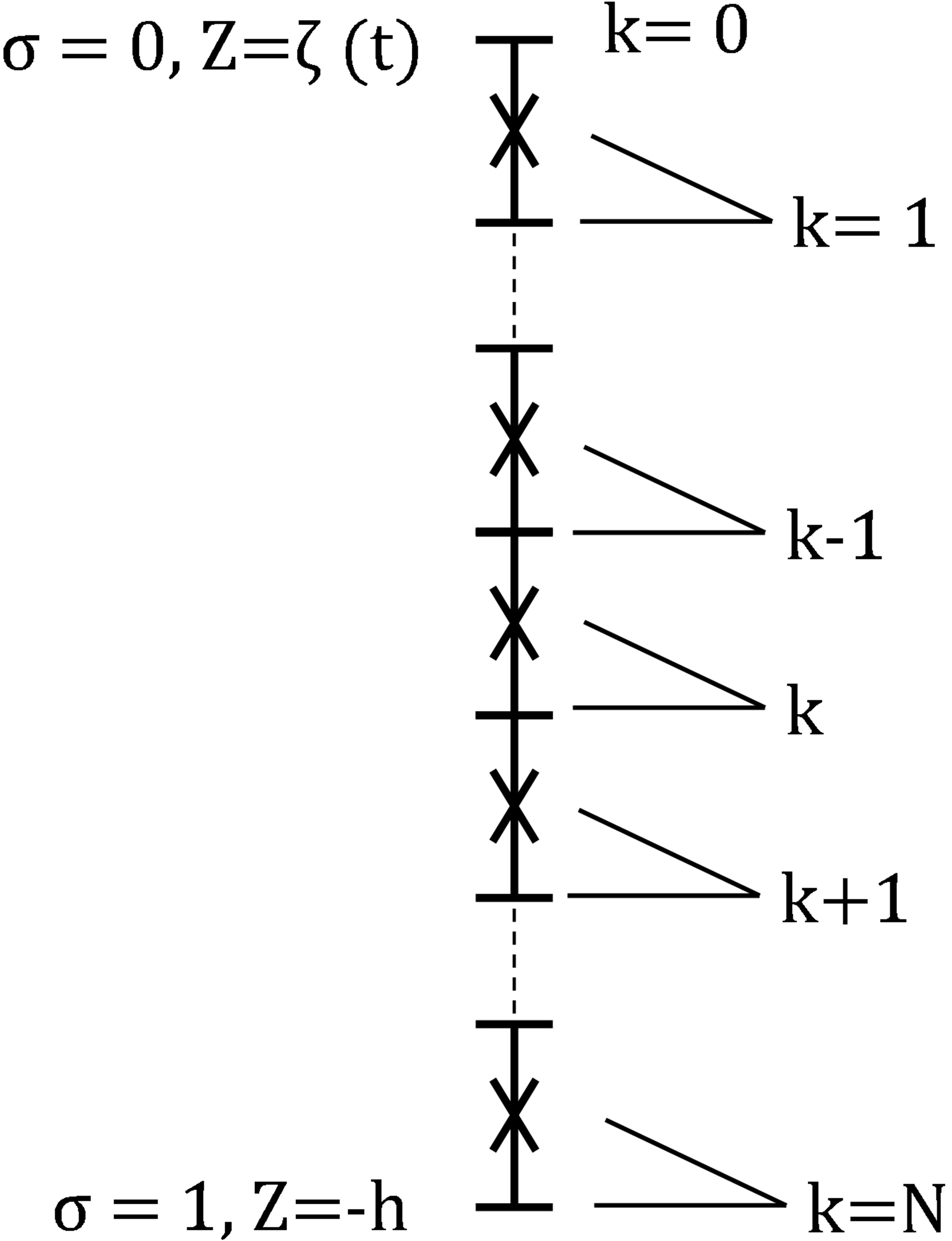
Figure 1 Spatial organization of σ vertical coordinate system.

2.2 The 3D apparent viscosity of fluid mud

K_m and A_m in Equations 2, 3 represent the vertical and horizontal diffusion coefficients of fluid, which represent the sum of the molecular viscosity and turbulent dissipation of the fluid. In the original version of the FVCOM model, K_m is calculated from the MY-2.5 turbulence model (Mellor and Yamada, 1982), and A_m is calculated from the Smagorinsky model (Smagorinsky, 1963). For water bodies with low sediment concentrations, the effect of molecular viscosity on fluid motion is much less than the effect of turbulence, so when the model uses a turbulence closure model to calculate K_m and A_m, the molecular viscosity can be ignored. However, for fluids with high sediment concentrations, such as fluid mud, which is a non-Newtonian fluid, its viscosity is much greater than that of a water body and cannot be neglected in the model simulation.

For the fluid mud, both K_m and A_m are equal to (Equation 7):

$\begin{array}{ll}{v}_a+v_{tur}& (7)\end{array}$

Where v_a is the apparent viscosity of fluid mud, and v_tur is the turbulent viscosity diffusion coefficient, which is calculated by turbulence models. For the laminar flow of fluid mud, only the apparent viscosity is taken into account. Therefore:

$\begin{array}{ll}{K}_m=A_m=v_a& (8)\end{array}$

Here, we employ the Herschel-Bulkley rheological model to calculate the apparent viscosity v_a because of its simplicity and wide applicability. It is suitable for characterizing fluid mud because it can be transformed into a Newtonian fluid, Bingham fluid, or shear-thinning fluid based on parameter variations (Coussot and Piau, 1994; Huang and García, 1998; Wurpts, 2005; Yang et al., 2015; Emami et al., 2020; Lovato et al., 2022; Lovato, 2023). The 1D form of the Herschel–Bulkley model is written as:

$\begin{array}{ll}\tau ={\tau }_0+K{(\frac{\partial u}{\partial z})}^n& (9)\end{array}$

where τ₀, K, and n are rheological parameters, τ₀ is the yield shear stress, K is the consistency coefficient, and n is the flow index. When n=1 and τ₀ = 0, the model represents a Newtonian fluid, and when n=1 and τ₀≠0, the model represents a Bingham fluid. The 3D form of Equation 9 is Equation 10:

$\begin{array}{ll}\tau =2\left\{K\sqrt{{(2I{I}_E)}^{n-1}}+\frac{{\tau }_0}{2I{I}_E}\right\}E& (10)\end{array}$

where τ is the three-dimensional stress tensor, which represents the shear stress on the fluid. E is the three-dimensional strain rate tensor, which represents the deformation of the fluid, and II_E is the second invariant deformation rate tensor, which is written as Equation 11:

$\begin{array}{ll}I{I}_E={(\frac{\partial u}{\partial x})}^2+{(\frac{\partial v}{\partial y})}^2+{(\frac{\partial w}{\partial z})}^2+\frac{1}{2}[{(\frac{\partial u}{\partial y}+\frac{\partial v}{\partial x})}^2+{(\frac{\partial u}{\partial z}+\frac{\partial w}{\partial x})}^2+{(\frac{\partial v}{\partial z}+\frac{\partial w}{\partial y})}^2]& (11)\end{array}$

Then, the apparent viscosity of the fluid mud can be expressed as Equation 12:

$\begin{array}{ll}{v}_a=(K\sqrt{{(2I{I}_E)}^{n-1}}+\frac{{\tau }_0}{\sqrt{2I{I}_E}})& (12)\end{array}$

In the terrain-following coordinate system, transforming II_E by coordinates yields Equation 13:

$\begin{array}{ll}I{I}_E={(\frac{\partial u}{\partial x})}^2+{(\frac{\partial v}{\partial y})}^2+{(\frac{1}{D}\frac{\partial w}{\partial \sigma })}^2+\frac{1}{2}[{(\frac{\partial u}{\partial y}+\frac{\partial v}{\partial x})}^2+{(\frac{1}{D}\frac{\partial u}{\partial \sigma }+\frac{\partial w}{\partial x})}^2+{(\frac{1}{D}\frac{\partial v}{\partial \sigma }+\frac{\partial w}{\partial y})}^2]& (13)\end{array}$

2.3 Numerical discretization for the 3D Herschel–Bulkley rheological model

The calculation of apparent viscosity requires a numerical discretization of the partial derivatives in Equation 13. Here, we use different discretization methods in the horizontal and vertical directions.

The horizontal discretization uses a spatial reconstruction method with second-order accuracy proposed by Kobayashi et al. (1999), as shown in Figure 2. The partial derivative of u at cell i are as follows Equation 14 and Equation 15:

Figure 2

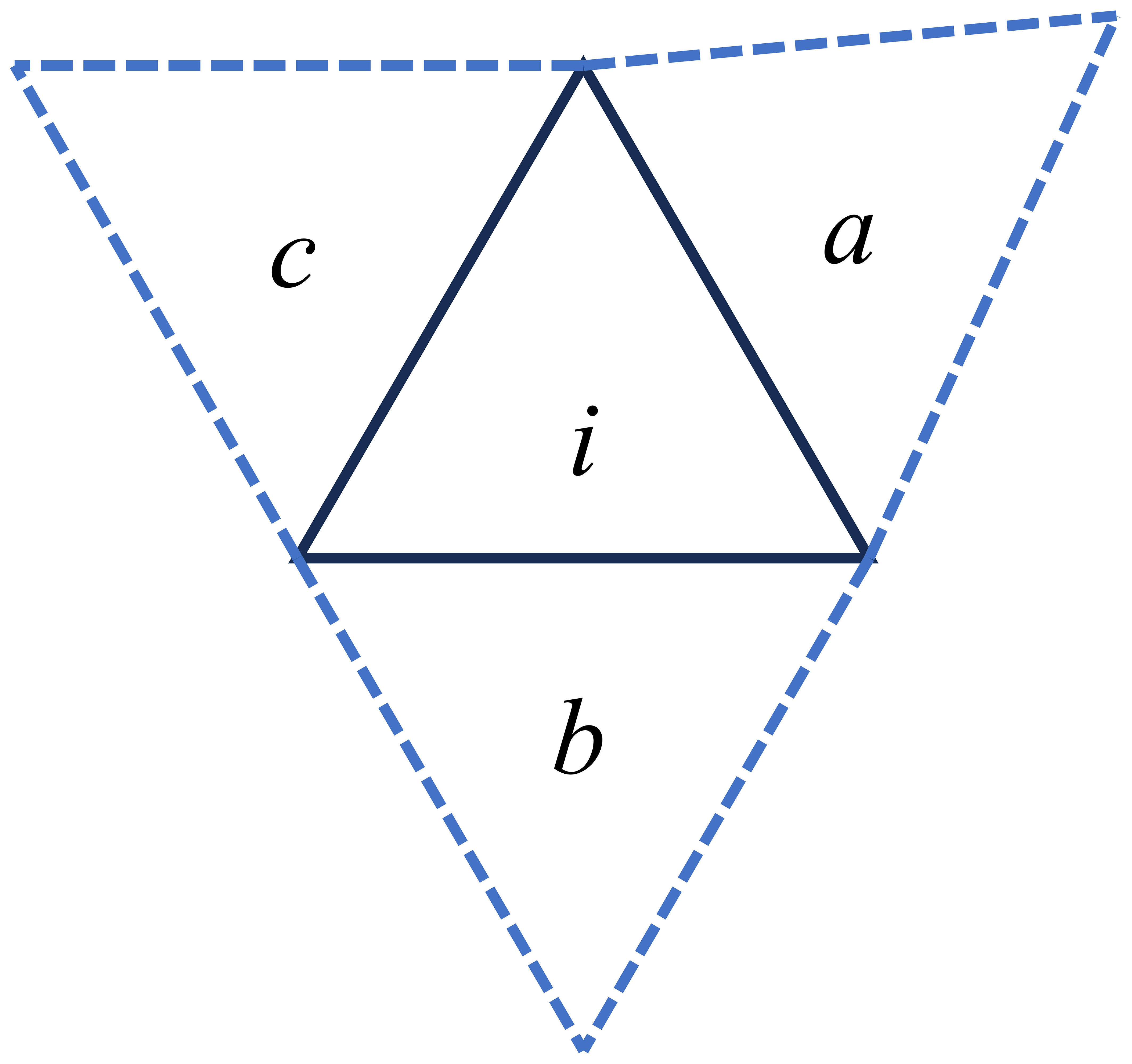
Figure 2 Schematic diagram of spatial reconstruction for partial derivatives on triangular grids. (i represents the cell where the partial derivative is located, a, b, and b represent the neighboring cells of the partial derivative cell.)

$\begin{array}{ll}\frac{\partial u}{\partial x}=\frac{{\displaystyle {\sum }_{j\in (a,b,c)}{y}_j(u_j-u_i){\displaystyle \sum x_j{y}_j-{\displaystyle {\sum }_{j\in (a,b,c)}{x}_j(u_j-u_i){\displaystyle \sum y_j^2}}}}}{{({\displaystyle {\sum }_{j\in (a,b,c)}{x}_j{y}_j})}^2-{\displaystyle {\sum }_{j\in (a,b,c)}{y}_j^2}{\displaystyle \sum x_j^2}}& (14)\end{array}$

$\begin{array}{ll}\frac{\partial u}{\partial y}=\frac{{\displaystyle {\sum }_{j\in (a,b,c)}{x}_j(u_j-u_i){\displaystyle \sum x_j{y}_j-{\displaystyle {\sum }_{j\in (a,b,c)}{y}_j(u_j-u_i){\displaystyle \sum x_j^2}}}}}{{({\displaystyle {\sum }_{j\in (a,b,c)}{x}_j{y}_j})}^2-{\displaystyle {\sum }_{j\in (a,b,c)}{y}_j^2}{\displaystyle \sum x_j^2}}& (15)\end{array}$

In the vertical direction, for the discretization of $\frac{\partial u}{\partial \sigma }$, the central differential approach is used.

The discretization at the surface layer is as Equation 16:

$\begin{array}{ll}{(\frac{\partial u}{\partial \sigma })}_k=\frac{(2u_k-\frac{2(u_k\Delta {\sigma }_{k+1}+u_{k+1}\Delta {\sigma }_k)}{\Delta {\sigma }_k+\Delta {\sigma }_{k+1}})}{\Delta {\sigma }_k}& (16)\end{array}$

The discretization at the bottom layer is as Equation 17:

$\begin{array}{ll}{(\frac{\partial u}{\partial \sigma })}_k=\frac{(\frac{2(u_k\Delta {\sigma }_{k-1}+u_{k-1}\Delta {\sigma }_k)}{\Delta {\sigma }_k+\Delta {\sigma }_{k-1}}-2u_k)}{\Delta {\sigma }_k}& (17)\end{array}$

The discretization at the central layer is as Equation 18:

$\begin{array}{ll}{(\frac{\partial u}{\partial \sigma })}_k=\frac{(\frac{u_k\Delta {\sigma }_{k-1}+u_{k-1}\Delta {\sigma }_k}{\Delta {\sigma }_k+\Delta {\sigma }_{k-1}}-\frac{u_k\Delta {\sigma }_{k+1}+u_{k+1}\Delta {\sigma }_k}{\Delta {\sigma }_k+\Delta {\sigma }_{k+1}})}{\Delta {\sigma }_k}& (18)\end{array}$

where u_k is the velocity at the center of layer k and Δσ_k is the difference in sigma coefficients at layer k.

The partial derivatives of velocity v and w are discretized in the same way.

3 Model validation

Two flume experiments with the gravity current of fluid mud were collected to validate the developed numerical model. For the simulation of these two experiments, although the 3D model is used, it behaves as a two-dimensional model in the x and z directions due to the geometry of the flume.

3.1 Comparison with van Kessel and Kranenburg’s experiment

The flume experiment was conducted to investigate the gravity current of fluid mud on a slope by van Kessel and Kranenburg (1996). Both the flow velocity profile and the density profile during the experiment were measured. The sketch of the experimental flume is shown in Figure 3, with a total length of 13.25 m, a depth of 0.72 m and a width of 0.5 m. The flume is filled with tap water, and the sediment is mixed with tap water in a mixing tank to produce fluid mud of fixed density. When the weir was lifted up to the desired height, a density current was generated, and the fluid mud flowed into the flume along the slope. The flow rate of the fluid mud was recorded by an electromagnetic velocity meter. The flow of the fluid mud was kept constant during the experiment, and a velocity meter and ultrasonic high-concentration meter (UHCM) were set up at p1 and p2, which were 1.27 m and 5.43 m away from the inlet, respectively. At the end of the flume, there is an overflow weir to ensure that the water level in the flume remains constant and a settling tank to recover the sediment for reuse.

Figure 3

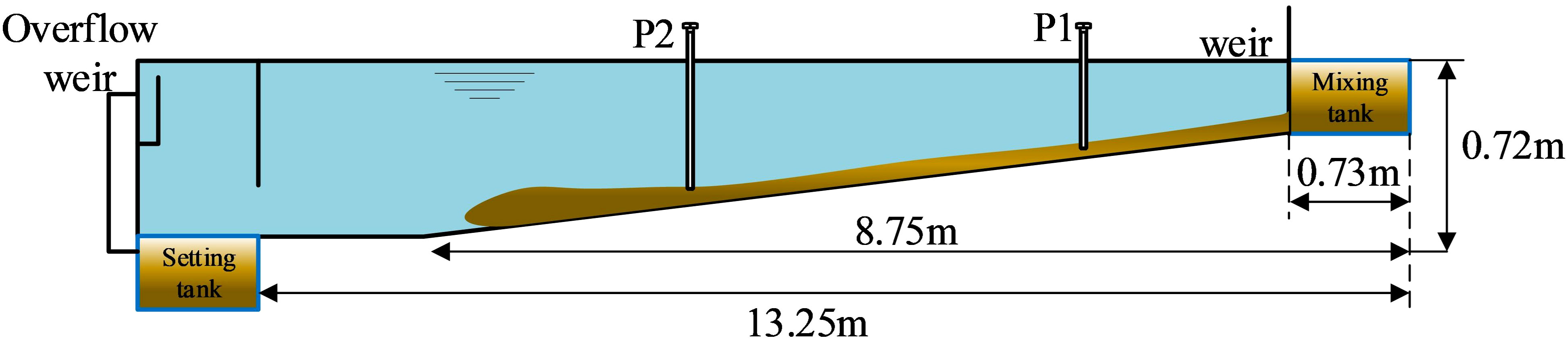
Figure 3 Schematic of the experimental setup after van Kessel and Kranenburg (1996).

The experiment gives the rheological parameters as a functionof sediment concentration (Equation 19 and Equation 20) based on Wan (1985):

$\begin{array}{ll}{\tau }_0=c_1{C}_v{}^{c_2}& (19)\end{array}$

$\begin{array}{ll}K={\mu }_w(1+c_3{C}_v{}^{c_4})& (20)\end{array}$

where C_v is the volume concentration of sediment, defined by Equation 21:

$\begin{array}{ll}{C}_v=\frac{\rho -{\rho }_w}{{\rho }_s-{\rho }_w}& (21)\end{array}$

where ${\rho }_w$ is the density of water and is the density of China-clay sediment (2,590 kg/m³). μ_w is the viscosity of the water, and the value 1.0e-03 was taken. c₁~c₄ are empirical coefficients, and according to the test, c₁ = 998, c₂ = 3, c₃ = 206 and c₄ = 1.68 were adopted. The experiment regarded the fluid mud as a Bingham fluid, and hence, the rheological parameter n=1.

Group 3 of the experiments was selected to validate the model. The density of the fluid mud was 1200 kg/m³, the bottom inlet height was 5 cm, the flow rate of the fluid mud into the tank was 0.004 m³/s, and the slope ratio was 1:42.6. The flow in this group of experiments was laminar. The mixing tank and the settling tank are omitted in the numerical model, and the computational domain is 12.52 m long, 0.72 m deep and 0.5 m wide.

The 800 computational cells are uniformly divided horizontally, with cell side lengths of 0.125 m, 100 layers are divided in the vertical direction, and the spatial resolution is gradually increased from the surface layer to the bottom, with a thickness of 0.01 m for the surface and 0.0008 m for the bottom. The experiment flume is set as solid wall boundary conditions. The water surface is set as a free water surface boundary condition, while the bottom is set as a movable roughness boundary condition. At the inlet where fluid mud flow enters, we set the same flow input conditions as the validation case. The main parameters of the model are shown in Table 1. Figure 4 shows the snapshot plots of the simulation results at 23 s, 40 s, 70 s and 80 s. In order to clearly depict the movement and distribution of fluid mud, as indicated by the vertical axis, the Figure 4 does not show the entire flume but instead focuses on a local area at a height of 0 below -0.2m. Furthermore, the right end of the horizontal axis was set as the starting position and labeled as 0 distance to maintain consistency with the experimental conditions. The fluid mud forms a gravity flow along the slope, arrives at the turning point of the slope to flatten at approximately 40 s, approaches the end of the flume at approximately 70 s, and reaches the end of the flume at approximately 80 s. Figure 5 shows a detailed view of the fluid mud head in Figure 4A at the region below the 0 height at -0.45 meters. The velocity and density profiles at the location of P1 are extracted after the head passed through. Figures 6A, B show the comparisons between the simulated density and velocity profile with respect to the measured data. It can be observed that the simulated results generally agree with the experimental data. The simulated density profile appears smoother compared to the experimental data, which is a result of the continuous modeling approach solving the advection-diffusion equation over an entire column. Figure 7 shows the viscosity distribution calculated in the model at the same moments as Figure 4. It can be observed that there is a significant variation in viscosity at the interface between the fluid mud and water. In the region where the fluid mud flows, the viscosity ranges from 0.001 to 0.1 m²/s, which is much higher than the viscosity of the water column.

Table 1

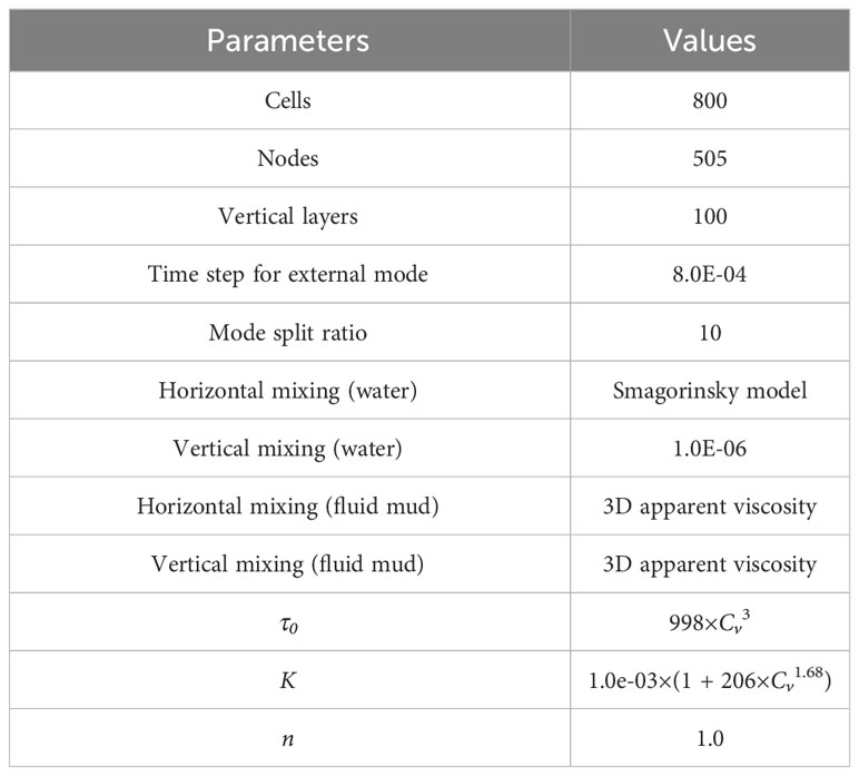
Table 1 The main parameters for simulation.

Figure 4

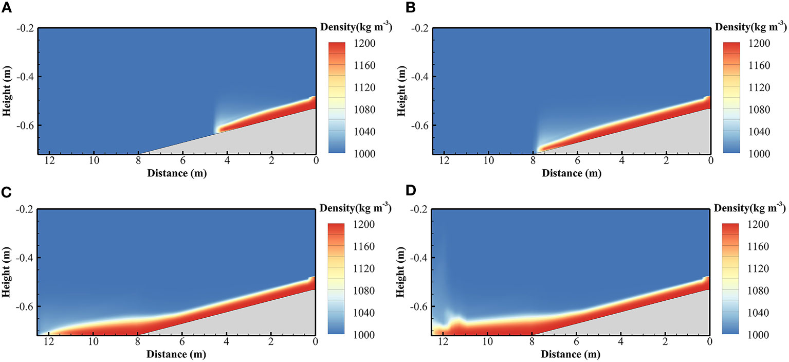
Figure 4 Snapshot of fluid mud movement (local area at a height of 0 below -0.2m, the right end of the horizontal axis was set as 0 distance): (A) at 23 seconds, (B) at 40 seconds, (C) at 70 seconds, and (D) at 80 seconds.

Figure 5

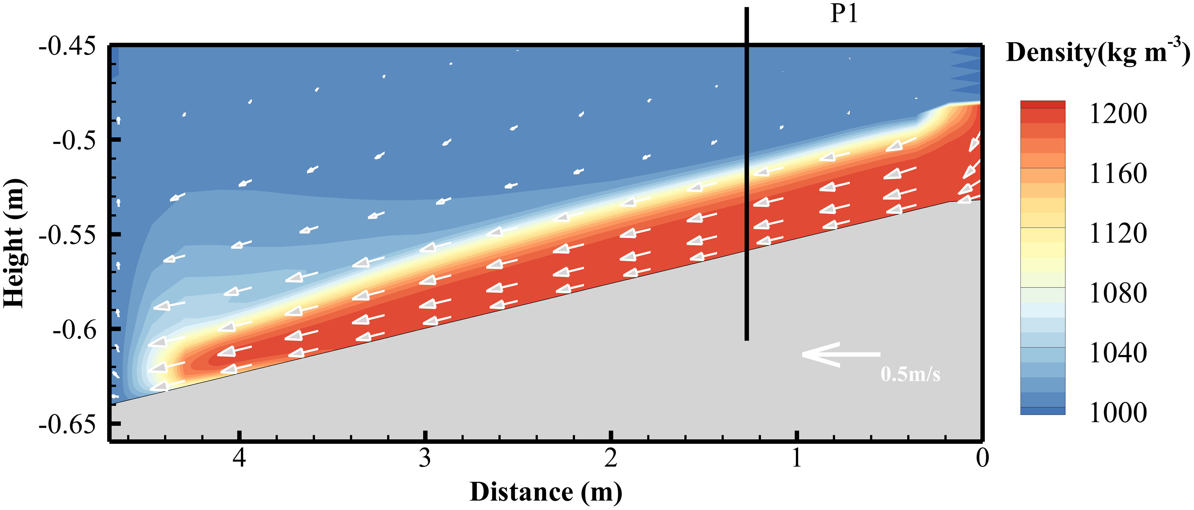
Figure 5 Detailed view of the head of the fluid mud of Figure 4A (local area at a height of 0 below -0.45m, the right end of the horizontal axis was set as 0 distance).

Figure 6

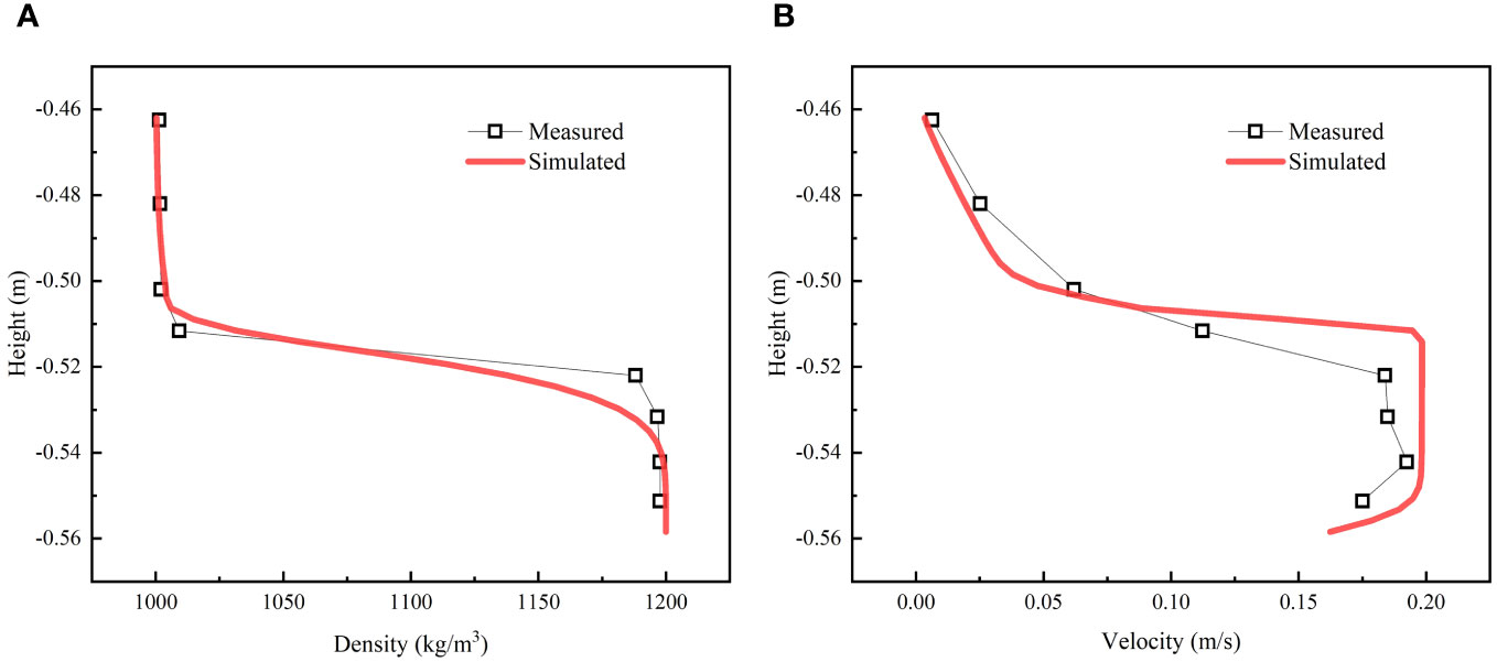
Figure 6 Density and velocity profile of position P1 at 23 s, (A) density profile; (B) velocity profile; the red line is the simulation results, squares is the measured data.

Figure 7

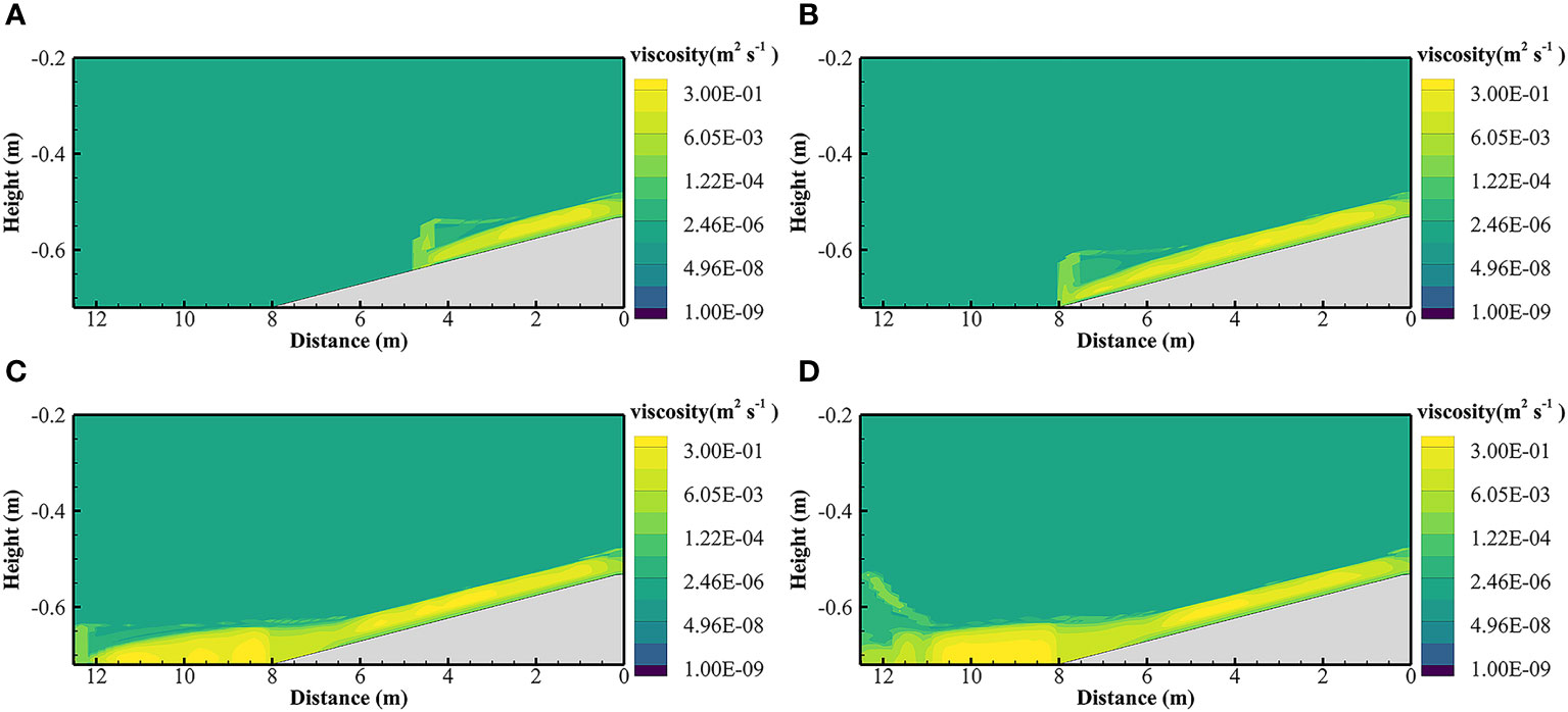
Figure 7 Distribution of viscosity at different moments: (A) at 23 s, (B) at 40 s, (C) at 70 s, and (D) at 80 s.

3.2 Comparison of simulation with Chowdhury and Testik’s experiment

Chowdhury and Testik (2012) investigated the gravity current of fluid mud in a flat sloping rectangular flume, and a schematic diagram of the flume is shown in Figure 8. The flume is 4.3 m long, 0.25 m deep and 0.5 m wide. The sediment was mixed with water through a mixing tank to form fluid mud with a fixed concentration and flowed out from the bottom of the flume at a constant flow rate. Two cameras were used to record the movement of the fluid mud, and the head position over time was obtained by image analysis algorithms. Rheological shear tests were also carried out, and the rheological parameters were fitted using power-law equations (ignoring yield stress) to obtain the following relationship between rheological parameters and sediment concentration (Equation 22 and Equation 23):

Figure 8

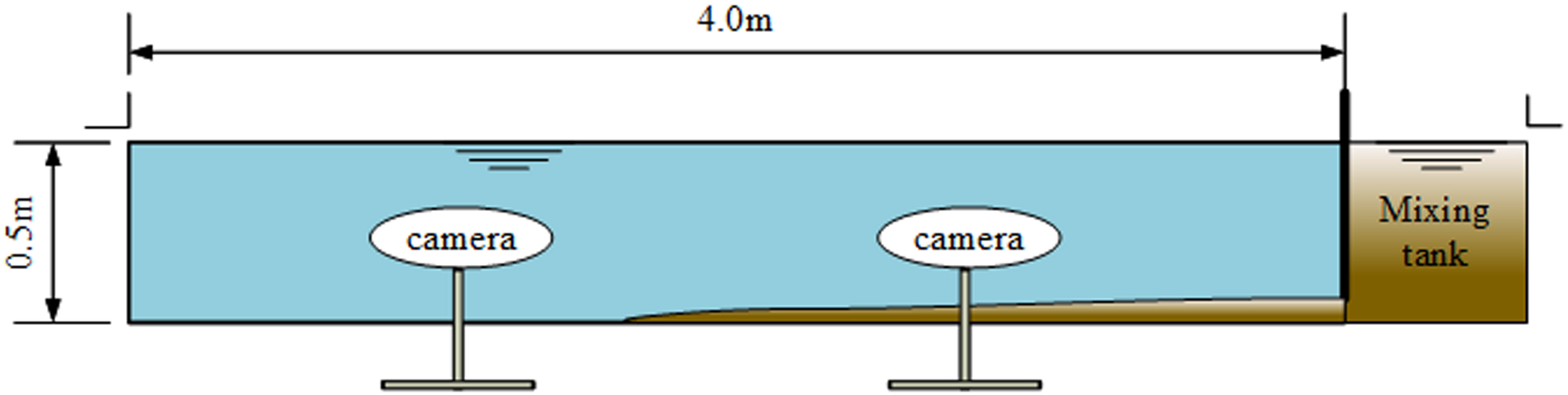
Figure 8 Schematic of the experimental setup after Chowdhury and Testik, 2012.

$\begin{array}{ll}K=0.8\times {10}^{-3}{C}_v^{3.39}& (22)\end{array}$

$\begin{array}{ll}n=1.03\times C_v^{-0.76}& (23)\end{array}$

Two groups of experiments with laminar flow were selected for simulation, and the experimental conditions are listed in Table 2. Exp01 is a Newtonian fluid with a low sediment concentration of 0.4%, and Exp02 is a non-Newtonian fluid with a high sediment concentration of 4.43%. The computational domain is uniformly divided into 3240 cells in the horizontal direction, and the side length of the cell is 0.025 m; the vertical direction is divided into 30 layers and gradually refined from the surface layer to the bottom layer. The thickness of the calculation cell in the surface layer is 0.026 m, and the thickness of the bottom calculation cell is 0.006 m. Similar to section 3.1, the same boundary condition is used. The main parameters used in the model are listed in Table 3.

Table 2

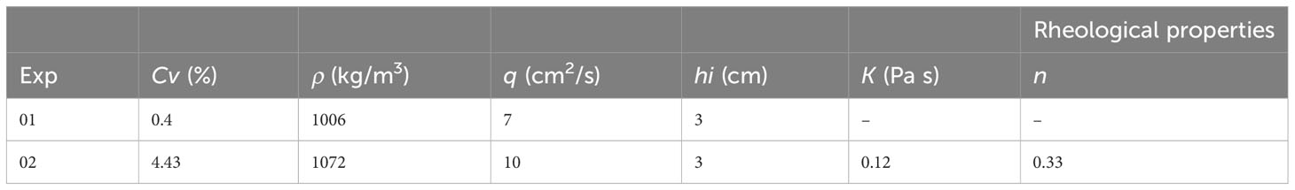
Table 2 Experimental conditions (Chowdhury and Testik, 2012).

Table 3

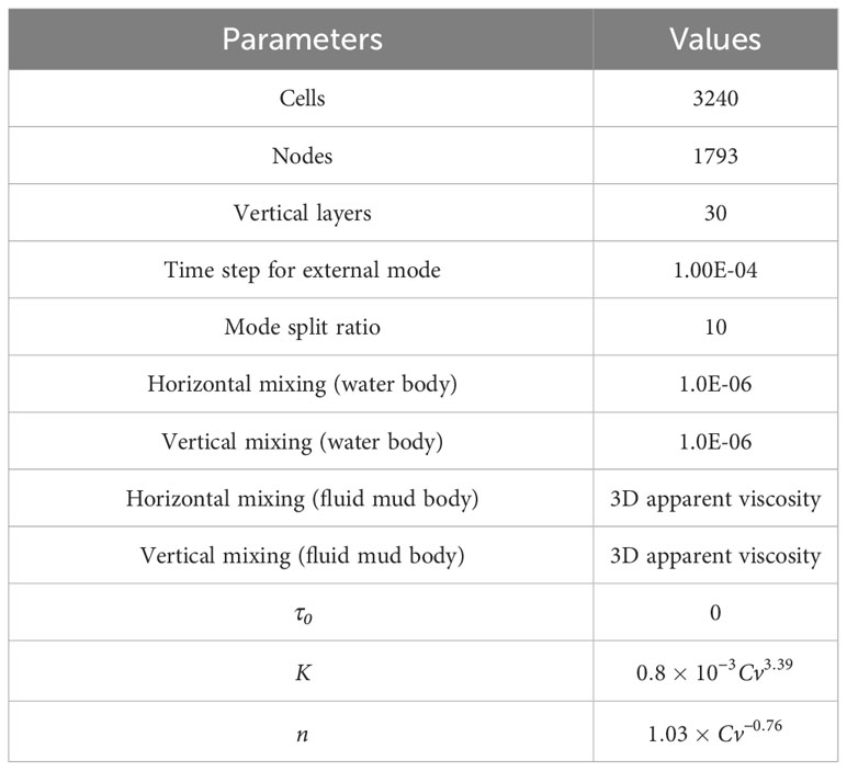
Table 3 The main parameters of the numerical model to simulate the experiment by Chowdhury and Testik (2012).

The simulated head positions of the fluid mud with time, together with the measured data, are shown in Figure 9. It can be seen that the fluid mud head of the non-Newtonian body with high sediment concentration travels faster than the Newtonian body with low sediment concentration; this is because the higher sediment concentration forms a greater density difference with the water body, thus forming a faster traveling gravity current. The simulation results are in good agreement with the experimental results.

Figure 9

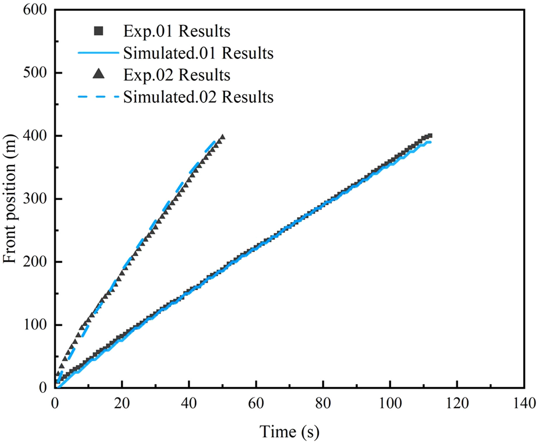
Figure 9 Front position of the head of fluid mud with time.

4 Discussion

To better understand the differences between 3D rheological model (referred to as the 3D model) and 1DV rheological model (referred to as the 1DV model), we compare the simulated results of fluid mud flows in this section. By converting the Herschel–Bulkley model into sigma coordinates, we obtained the apparent viscosity v_av of the 1DV model (Equation 24):

$\begin{array}{ll}{v}_{av}=K{(\frac{\partial u}{\partial \sigma }*\frac{1}{D})}^{n-1}+\frac{{\tau }_0}{\frac{\partial u}{\partial \sigma }*\frac{1}{D}}& (24)\end{array}$

To incorporating the 1DV apparent viscosity ${\nu }_{av}$ into the momentum Equations 2, 3, the Equation 8 is no longer applicable as v_av only represents the apparent viscosity in the vertical direction. Therefore, we modify it as Equation 25:

$\begin{array}{ll}\begin{array}{c}{K}_m={\nu }_{av}\end{array}& (25)\end{array}$

4.1 Comparison of 3D model and 1DV model for flume experiment

We applied the1DV rheological model to simulate the experiment by van Kessel and Kranenburg (1996) in Section 3.1. Figure 10 illustrates the simulated movement of the fluid mud, showing a similarity to the results by 3D model in Section 3.1. Figure 11 compares the 1DV and 3D models with the experimental monitoring data and shows the differences in velocity profiles and density. From the simulation results, the 1DV model, which only considers the velocity shear ∂u/∂σ, also can simulate the movement of fluid mud along the slope. However, the 3D model, which accounts for velocity shears in all directions, still exhibits some differences compared to the 1DV model, and compares better with the observations.

Figure 10

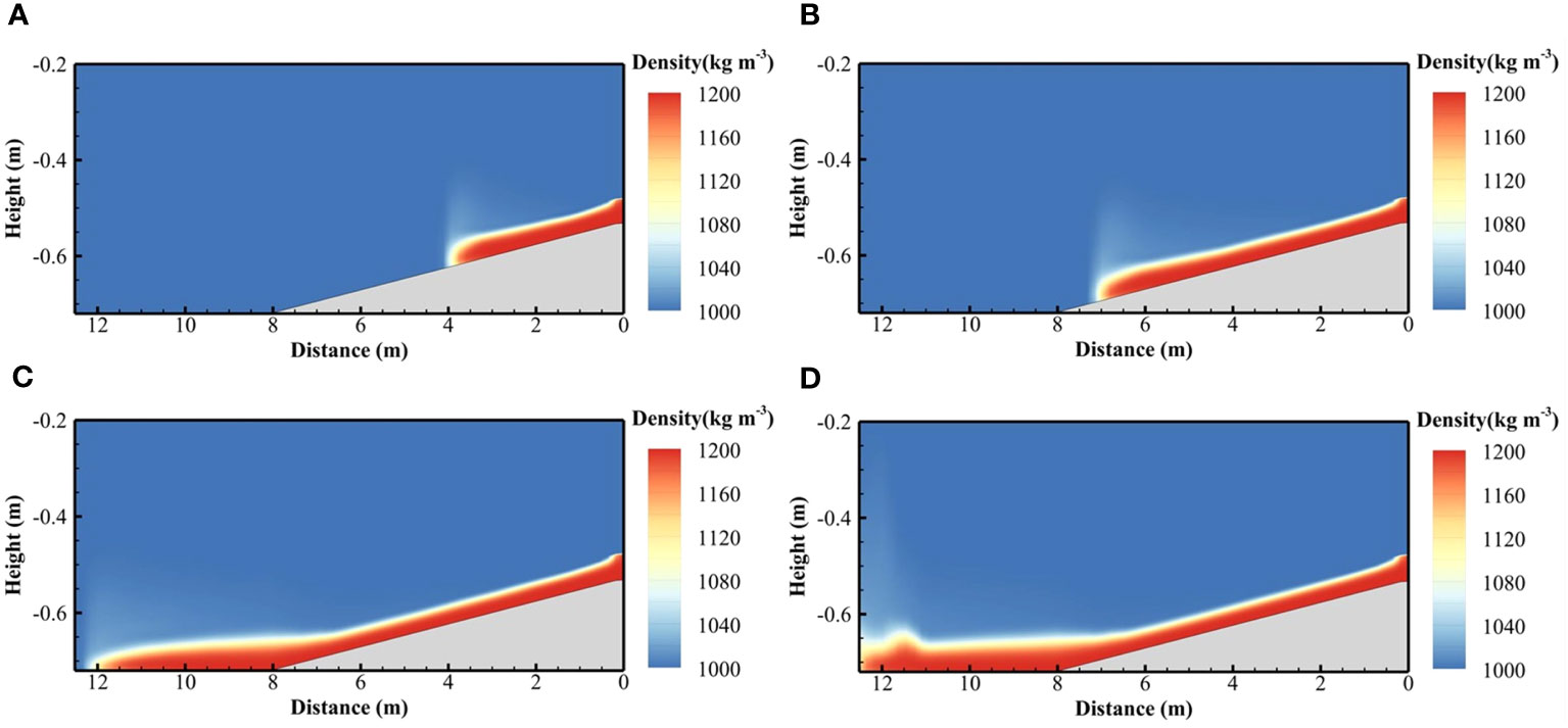
Figure 10 Snapshot of fluid mud movement by 1DV Herschel–Bulkley model: (A) at 23 s, (B) at 40 s, (C) at 70 s, and (D) at 80 s.

Figure 11

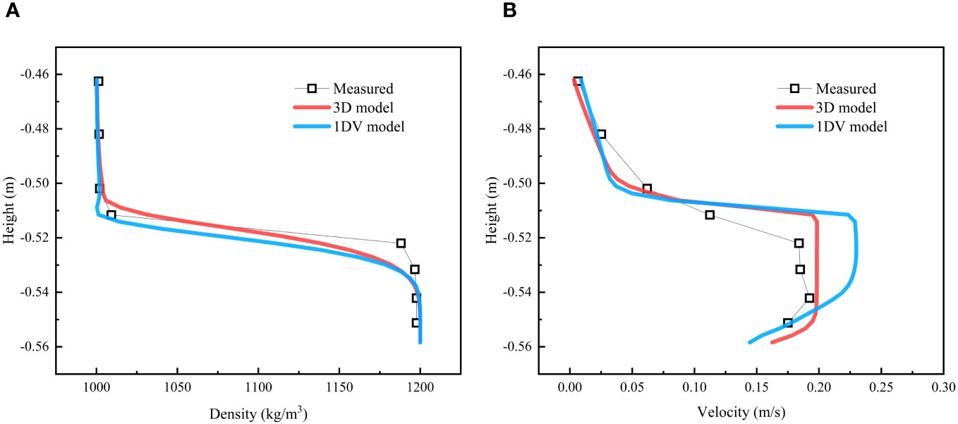
Figure 11 Density and velocity profile of position P1 at 23 s, (A) density profile; (B) velocity profile; the red line is the simulation results by 3D Herschel–Bulkley model; the bule line is the simulation results by 1DV Herschel–Bulkley model; Squares are the measured data.

Due to the constraints of the flume boundary in the experimental cases, the calculated results primarily reflect the effect of apparent viscosity in the vertical direction, and do not fully demonstrate the differences in simulation results between the 3D model and the 1DV model.

4.2 Comparison for fluid mud flow in idealized flume-basin

To further compare the differences in simulation results between the two models, we established an idealized flume-basin case based on the experiments conducted by Kessel in 1996. As shown in Figure 12, the flat part of the flume is widened and lengthened so that a truly three-dimensional fluid mud flow in the basin (widened part of the flume) can be formed. The computational domain was divided into 25004 cells in the horizontal direction and 100 layers in the vertical direction (gradually refined from the surface to the bottom). The spatial resolution of the grid and the parameters used in the rheological model were the same as those described in Section 3.1.

Figure 12

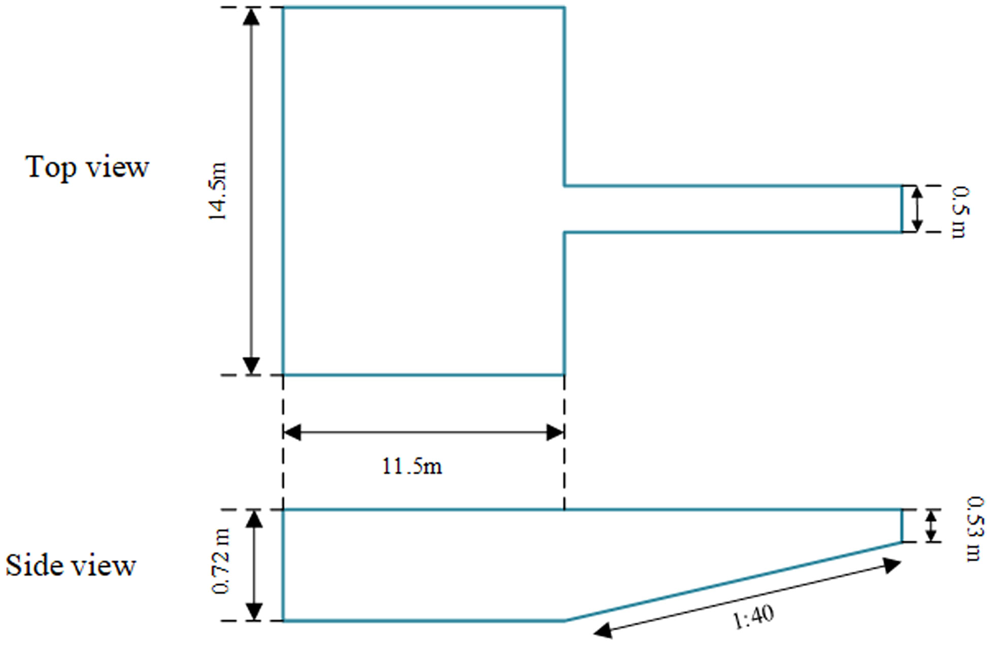
Figure 12 A hypothetical case based on the Kessel experiment (the flat slope of the flume is lengthened and widened).

We used density contour lines at 1030 kg/m³ to indicate the position of fluid mud movement. As shown in Figure 13, it displays the fluid mud movement from both the top view and side view. It can be observed that at 30 seconds and 40 seconds, the simulation results of the two models in the flume are not significantly different. However, after the fluid mud enters the basin at 100 seconds and 180 seconds, there are noticeable differences in the simulation results of the two models in the upper, middle, and lower layers of the fluid mud.

Figure 13

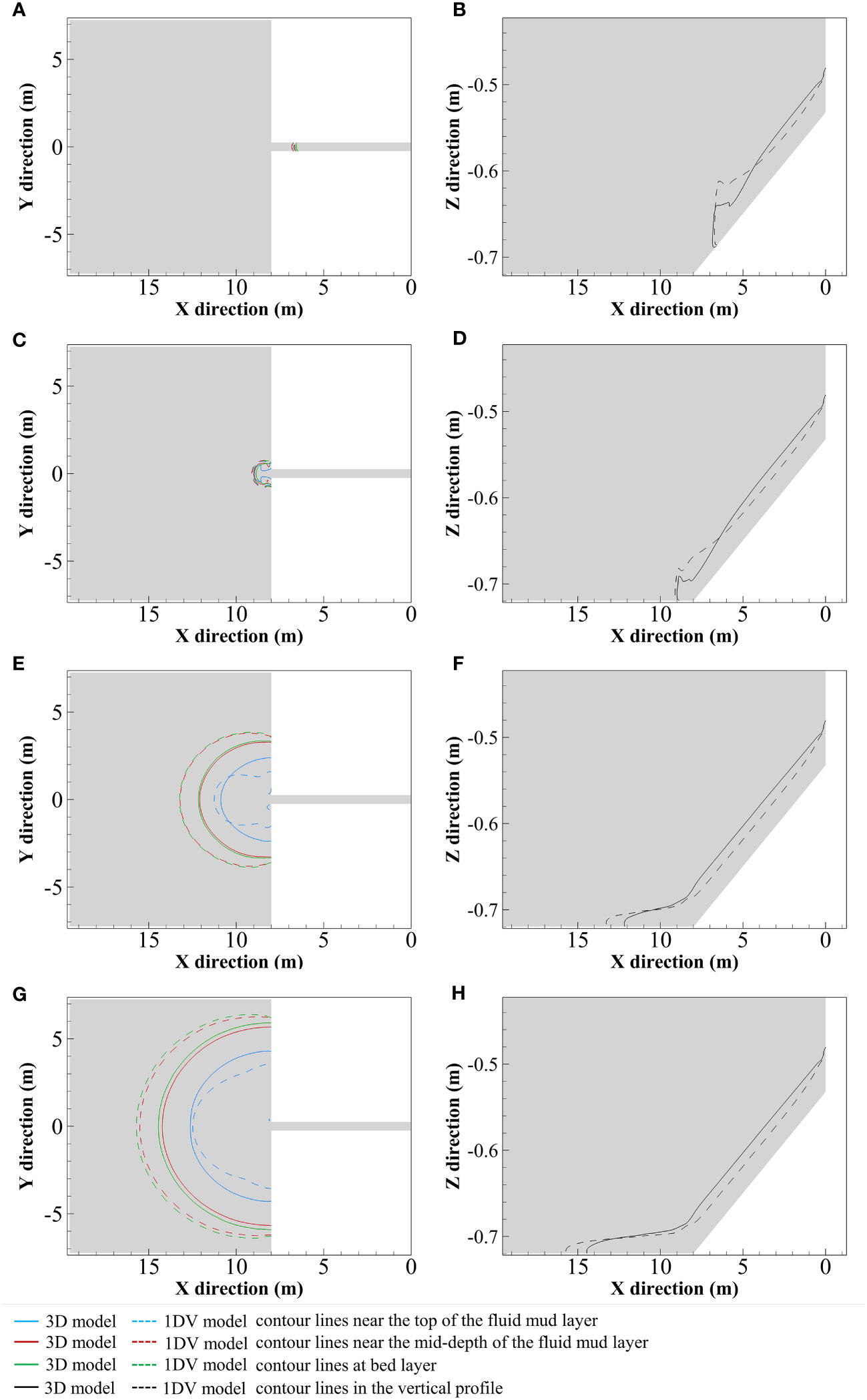
Figure 13 Contour lines plots of density 1030 kg/m³ at different moments: (A, C, E, G) are the horizontal distributions at 30 s, 40 s, 100 s, 180 s; (B, D, F, H) are the profile distributions along the centerline at 30 s, 40 s, 100 s, 180 s.

Figure 14 presents a further analysis of the positional variations at the head of the fluid mud along the centerline and at a 45° angle, as simulated by both models. It can be observed that as the simulation time increases, the differences of position between the two models gradually become more prominent. Figure 15 displays the horizontal viscosity diffusion at the bottom of the fluid mud at the same time as Figure 13. It can be seen that the 3D model, which takes into account the apparent viscosity in horizontal direction, produces significantly different results from the 1DV model, especially after the fluid mud enters the basin.

Figure 14

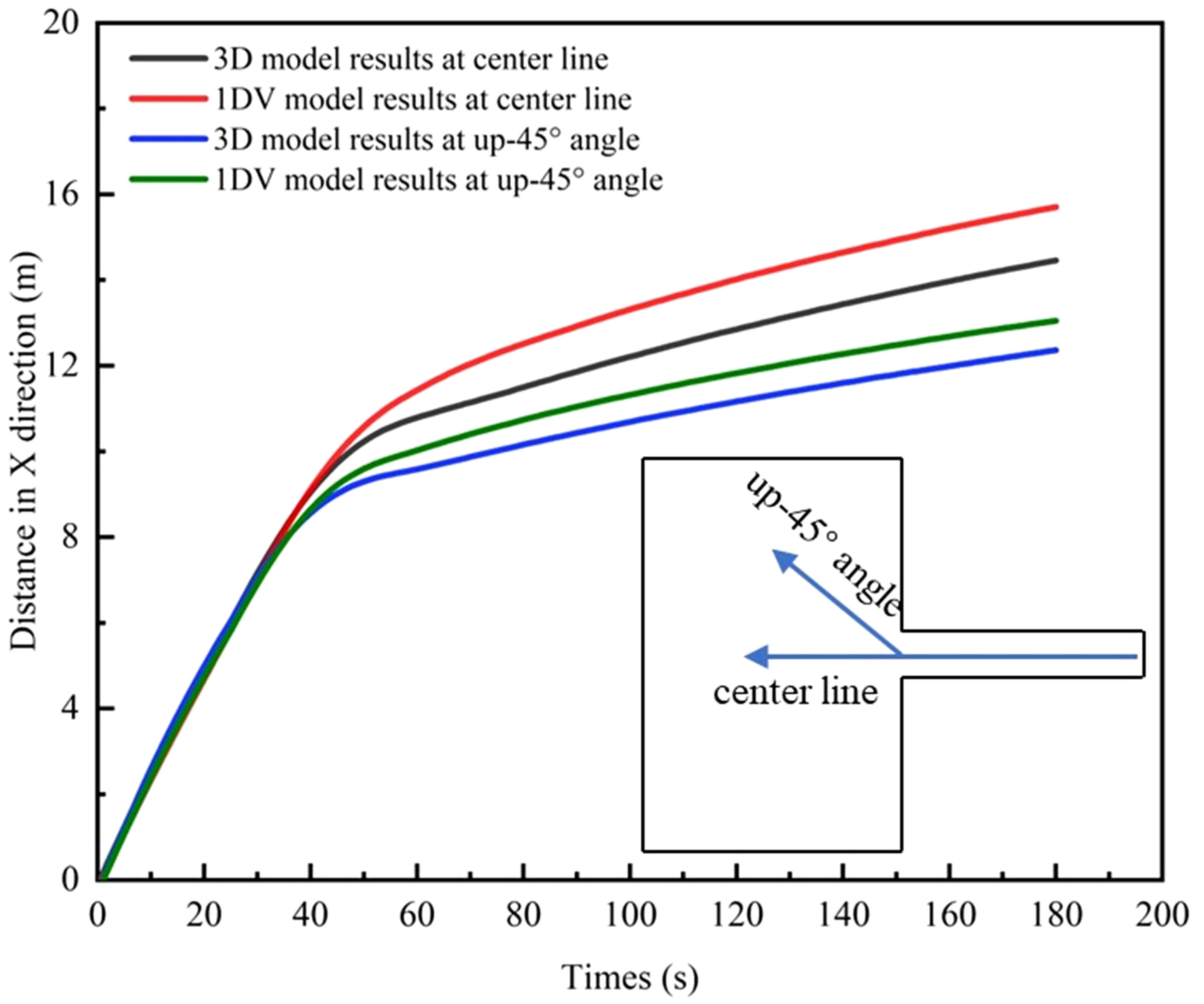
Figure 14 Variation in the front position of fluid mud in the x direction with time.

Figure 15

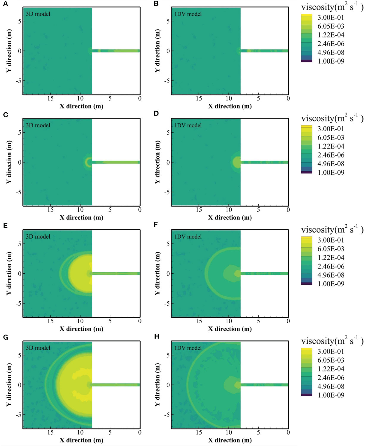
Figure 15 Distribution of viscosity in horizontal direction on the bottom layer: (A, C, E, G) are the results of the 3D model at 30 s, 40 s, 100 s 180 s (B, D, F, H) are the results of the 1DV model at 30 s, 40 s, 100 s 180 s.

The comparison results in this section indicate that the apparent viscosity in the horizontal direction has a significant influence on the simulation results, which is not considered in the 1DV model.

5 Conclusion

In this paper, a 3D Herschel–Bulkley rheological model was introduced into the FVCOM with a terrain-following coordinate system to calculate the apparent viscosity of the fluid mud. The developed model is verified by two water flume experiments on fluid mud. The simulation results show that the developed numerical model can simulate fluid mud with obvious non-Newtonian properties.

A comparison between the 1DV and the 3D rheological model in simulating the fluid mud motion shows that the results of the 3D model and the 1DV model have obvious differences, illustrates the significant impact of considering the apparent viscosity in horizontal direction on the simulation results, which 3D rheological model has taken into account.

The numerical model developed in this paper is able to describe the motion of the fluid mud and the continuous transition from Newtonian to non-Newtonian fluid. Future work will be built on this with a turbulent flow model for non-Newtonian fluid, allowing further description of the motion of fluid mud in a turbulent flow regime.

Data availability statement

The original contributions presented in the study are included in the article/supplementary material. Further inquiries can be directed to the corresponding author.

Author contributions

GS: Investigation, Software, Validation, Writing – original draft. JZ: Funding acquisition, Supervision, Writing – review & editing. QZ: Conceptualization, Funding acquisition, Supervision, Writing – review & editing. ZZ: Resources, Writing – review & editing. BY: Writing – review & editing. HY: Writing – review & editing.

Funding

The author(s) declare financial support was received for the research, authorship, and/or publication of this article. This research was financial supported by the National Key Research and Development Project of China (2021YFB2601100) and the National Natural Science Foundation of China (51979190; U1906231).

Acknowledgments

We gratefully appreciate Dr. Mijanur R. Chowdhury and Professor Wang Zhengbing for providing the experimental data in Section 3.2 and the technical report (Wang and Winterwerp, 1992), respectively.

Conflict of interest

The authors declare that the research was conducted in the absence of any commercial or financial relationships that could be construed as a potential conflict of interest.

Publisher’s note

All claims expressed in this article are solely those of the authors and do not necessarily represent those of their affiliated organizations, or those of the publisher, the editors and the reviewers. Any product that may be evaluated in this article, or claim that may be made by its manufacturer, is not guaranteed or endorsed by the publisher.

References

Azhikodan G., Yokoyama K. (2018). Sediment transport and fluid mud layer formation in the macro-tidal Chikugo river estuary during a fortnightly tidal cycle. Estuarine Coast. Shelf Sci. 202, 232–245. doi: 10.1016/j.ecss.2018.01.002

CrossRef Full Text | Google Scholar

Becker M., Schrottke K., Bartholomä A., Ernstsen V., Winter C., Hebbeln D. (2013). Formation and entrainment of fluid mud layers in troughs of subtidal dunes in an estuarine turbidity zone: dynamics of fluid mud in dune troughs. J. Geophys. Res. Oceans 118, 2175–2187. doi: 10.1002/jgrc.20153

CrossRef Full Text | Google Scholar

Chen C., Beardsley R. C., Cowles G., Qi J., Lai Z., Gao G., et al. (2012). An unstructured-grid, finite-volume community ocean model: FVCOM user manual (Cambridge, MA, USA: Sea Grant College Program, Massachusetts Institute of Technology).

Google Scholar

Chen C., Liu H., Beardsley R. C. (2003). An unstructured grid, finite-volume, three-dimensional, primitive equations ocean model: application to coastal ocean and estuaries. J. Atmos. Oceanic Technol. 20, 159–186. doi: 10.1175/1520-0426(2003)020<0159:AUGFVT>2.0.CO;2

CrossRef Full Text | Google Scholar

Chmiel O., Naulin M., Malcherek A. (2021). Combining turbulence and mud rheology in a conceptual 1DV model – an advanced continuous modeling concept for fluid mud dynamics. Die Küste 89, 1–27. doi: 10.18171/1.089101

CrossRef Full Text | Google Scholar

Chowdhury M. R., Testik F. Y. (2012). Viscous propagation of two-dimensional non-Newtonian gravity currents. Fluid Dyn. Res. 44, 45502. doi: 10.1088/0169-5983/44/4/045502

CrossRef Full Text | Google Scholar

Chung D. H. (1998). Numerical simulation of fluid mud layer under current and waves in estuaries and coastal areas. Vietnam J. Mech. 20, 5–15. doi: 10.15625/0866-7136/10023

CrossRef Full Text | Google Scholar

Coussot P., Piau J. M. (1994). On the behavior of fine mud suspensions. Rheola Acta 33, 175–184. doi: 10.1007/BF00437302

CrossRef Full Text | Google Scholar

Deltares (2021). Delft3d-flow simulation of multi-dimensional hydrodynamic flows and transport phenomena, including sediments, user manual hydro-morphodynamics (Delft, Netherlands: Deltares).

Google Scholar

Emami S.-M.-K., Mousavi S.-F., Hosseini K., Fouladfar H., Mohammadian M. (2020). Comparison of different turbulence models in predicting cohesive fluid mud gravity current propagation. Int. J. Sediment Res. 35, 504–515. doi: 10.1016/j.ijsrc.2020.03.010

CrossRef Full Text | Google Scholar

Ge J., Chen C., Wang Z. B., Ke K., Yi J., Ding P. (2020). Dynamic response of the fluid mud to a tropical storm. JGR Oceans 125. doi: 10.1029/2019JC015419

CrossRef Full Text | Google Scholar

Guan W. B., Kot S. C., Wolanski E. (2005). 3-D fluid-mud dynamics in the jiaojiang estuary, China. Estuarine Coast. Shelf Sci. 65, 747–762. doi: 10.1016/j.ecss.2005.05.017

CrossRef Full Text | Google Scholar

Hir P. L., Cayocca F. (2002). “3D application of the continuous modelling concept to mud slides in open seas,” in Proceedings in Marine Science. (Elsevier), 545–562. doi: 10.1016/S1568-2692(02)80039-0

CrossRef Full Text | Google Scholar

Huang X., García M. H. (1998). A Herschel–Bulkley model for mud flow down a slope. J. Fluid Mechanics 374, 305–333. doi: 10.1017/S0022112098002845

CrossRef Full Text | Google Scholar

James N., Adams J., Connell A., Lamberth S., MacKay C., Snow G., et al. (2020). High flow variability and storm events shape the ecology of the mbhashe estuary, South Africa. Afr. J. Aquat. Sci. 45, 131–151. doi: 10.2989/16085914.2020.1733472

CrossRef Full Text | Google Scholar

Kineke G. C., Sternberg R. W. (1995). Distribution of fluid muds on the amazon continental shelf. Mar. Geology 125, 193–233. doi: 10.1016/0025-3227(95)00013-O

CrossRef Full Text | Google Scholar

Kineke G. C., Sternberg R. W., Trowbridge J. H., Geyer W. R. (1996). Fluid-mud processes on the amazon continental shelf. Continental Shelf Res. 16, 667–696. doi: 10.1016/0278-4343(95)00050-X

CrossRef Full Text | Google Scholar

Kirby R. (1988). “High concentration suspension (fluid mud) layers in estuaries,” in Physical Processes in Estuaries. Eds. Dronkers J., van Leussen W. (Berlin, Heidelberg: Springer), 463–487. doi: 10.1007/978-3-642-73691-9_23

CrossRef Full Text | Google Scholar

Knoch D., Malcherek A. (2011). A numerical model for simulation of fluid mud with different rheological behaviors. Ocean Dynamics 61, 245–256. doi: 10.1007/s10236-010-0327-x

CrossRef Full Text | Google Scholar

Kobayashi M. H., Pereira J. M. C., Pereira J. C. F. (1999). A conservative finite-volume second-order-accurate projection method on hybrid unstructured grids. J. Comput. Phys. 150, 40–75. doi: 10.1006/jcph.1998.6163

CrossRef Full Text | Google Scholar

Le Hir P., Bassoullet P., Jestin H. (2000). “Application of the continuous modeling concept to simulate high-concentration suspended sediment in a macrotidal estuary,” in Proceedings in Marine Science. (Elsevier), 229–247. doi: 10.1016/S1568-2692(00)80124-2

CrossRef Full Text | Google Scholar

Lovato S. (2023) Sailing through fluid mud: Verification and Validation of a CFD model for simulations of ships sailing in muddy areas. Available at: http://resolver.tudelft.nl/uuid:b2156264-39f4-4a8d-a34d-35e5a21d38e9 (Accessed October 27, 2023).

Google Scholar

Lovato S., Kirichek A., Toxopeus S. L., Settels J. W., Keetels G. H. (2022). Validation of the resistance of a plate moving through mud: CFD modelling and towing tank experiments. Ocean Eng. 258, 111632. doi: 10.1016/j.oceaneng.2022.111632

CrossRef Full Text | Google Scholar

McAnally W. H., Friedrichs C., Hamilton D., Hayter E., Shrestha P., Rodriguez H., et al. (2007a). Management of fluid mud in estuaries, bays, and lakes. I present state of understanding on character and behavior. J. Hydraul. Eng. 133, 9–22. doi: 10.1061/(ASCE)0733-9429(2007)133:1(9

CrossRef Full Text | Google Scholar

McAnally W. H., Teeter A., Schoellhamer D., Friedrichs C., Hamilton D., Hayter E., et al. (2007b). Management of fluid mud in estuaries, bays, and lakes. II: measurement, modeling, and management. J. Hydraul. Eng. 133, 23–38. doi: 10.1061/(ASCE)0733-9429(2007)133:1(23

CrossRef Full Text | Google Scholar

Mellor G. L., Yamada T. (1982). Development of a turbulence closure model for geophysical fluid problems. Rev. Geophys. 20, 851. doi: 10.1029/RG020i004p00851

CrossRef Full Text | Google Scholar

Normant C. L. (2000). Three-dimensional modelling of cohesive sediment transport in the loire estuary. Hydrological Processes 14, 2231–2243. doi: 10.1002/1099-1085(200009)14:13<2231::AID-HYP25>3.0.CO;2-#

CrossRef Full Text | Google Scholar

Oberrecht D. (2021). Development of a numerical modeling approach for large-scale fluid mud flow in estuarine environments. Doctoral Thesis. (Hannover, Germany: LUH). doi: 10.15488/10488

CrossRef Full Text | Google Scholar

Odd N. V. M., Cooper A. J. (1989). A two-dimensional model of the movement of fluid mud in a high energy turbid estuary. J. Coast. Res. 185–193.

Google Scholar

Reide Corbett D., Dail M., McKee B. (2007). High-frequency time-series of the dynamic sedimentation processes on the western shelf of the mississippi river delta. Continental Shelf Res. 27, 1600–1615. doi: 10.1016/j.csr.2007.01.025

CrossRef Full Text | Google Scholar

Roberts W. (1993). Development of a mathematical model of fluid mud in the coastal zone. Proc. Institution Civil Engineers - Water Maritime Energy 101, 173–181. doi: 10.1680/iwtme.1993.24582

CrossRef Full Text | Google Scholar

Schmidt J., Malcherek A. (2021). Using a holistic modeling approach to simulate mud-induced periodic stratification in hyper-turbid estuaries. Geophysical Res. Lett. 48. doi: 10.1029/2021GL092798

CrossRef Full Text | Google Scholar

Shi J. Z. (2010). Tidal resuspension and transport processes of fine sediment within the river plume in the partially-mixed changjiang river estuary, China: a personal perspective. Geomorphology 121, 133–151. doi: 10.1016/j.geomorph.2010.04.021

CrossRef Full Text | Google Scholar

Smagorinsky J. (1963). General circulation experiments with the primitive equations: i. the basic experiment*. Mon. Wea. Rev. 91, 99–164. doi: 10.1175/1520-0493(1963)091<0099:GCEWTP>2.3.CO;2

CrossRef Full Text | Google Scholar

Traykovski P., Geyer R., Sommerfield C. (2004). Rapid sediment deposition and fine-scale strata formation in the hudson estuary: hudson estuary sediment deposition. J. Geophys. Res. 109, n/a–n/a. doi: 10.1029/2003JF000096

CrossRef Full Text | Google Scholar

Trowbridge J. H., Kineke G. C. (1994). Structure and dynamics of fluid muds on the amazon continental shelf. J. Geophys. Res. 99, 865. doi: 10.1029/93JC02860

CrossRef Full Text | Google Scholar

Van Haaren Y. (1995) Erosion of a fluid mud layer due to entrainment: numerical modelling. Available at: https://repository.tudelft.nl/islandora/object/uuid%3A9599aa9a-1ee3-4709-97e1-7b4c26abd5f3 (Accessed January 18, 2023).

Google Scholar

van Kessel T., Kranenburg C. (1996). Gravity current of fluid mud on sloping bed. J. Hydraulic Eng. 122, 710–717. doi: 10.1061/(ASCE)0733-9429(1996)122:12(710

CrossRef Full Text | Google Scholar

Wan Z. (1985). Bed material movement in hyperconcentrated flow. J. Hydraulic Eng. 111, 987–1002. doi: 10.1061/(ASCE)0733-9429(1985)111:6(987

CrossRef Full Text | Google Scholar

Wang L., Winter C., Schrottke K., Hebbeln D., Bartholomä A. (2008)Modelling of estuarine fluid mud evolution in troughs of large subaequous dunes. In: (Technische Universität Darmstadt). Available at: https://publications.marum.de/1648/ (Accessed March 6, 2023).

Google Scholar

Wang Z. B., Winterwerp J. C. (1992). A model to simulate the transport of fluid mud (Delft, The Netherlands: WL | Delft Hydraulics).

Google Scholar

Wilcox D. C. (1988). Reassessment of the scale-determining equation for advanced turbulence models. AIAA J. 26, 1299–1310. doi: 10.2514/3.10041

CrossRef Full Text | Google Scholar

Winterwerp J. C., Wang Z. B., van Kester J. A., Th. M., Verweij J. F. (2002). Far-field impact of water injection dredging in the crouch river. Proc. Institution Civil Engineers - Water Maritime Eng. 154, 285–296. doi: 10.1680/wame.2002.154.4.285

CrossRef Full Text | Google Scholar

Wu H., Wang Y. P., Gao S., Xing F., Tang J., Chen D. (2022). Fluid mud dynamics in a tide-dominated estuary: a case study from the yangtze river. Continental Shelf Res. 232, 104623. doi: 10.1016/j.csr.2021.104623

CrossRef Full Text | Google Scholar

Wurpts R. (2005). 15 years experience with fluid mud: definition of the nautical bottom with rheological parameters. Terra Aqua 99(Jun), 22–32.

Google Scholar

Yang X., Zhang Q., Hao L. (2015). Numerical investigation of fluid mud motion using a three-dimensional hydrodynamic and two-dimensional fluid mud coupling model. Ocean Dynamics 65, 449–461. doi: 10.1007/s10236-015-0815-0

CrossRef Full Text | Google Scholar