Simulation of sonar reverberation signal considering the ocean multipath and Doppler effect

Zhang, Sen; Wu, Jian; Yin, Tianqi

doi:10.3389/fmars.2023.1279693

ORIGINAL RESEARCH article

Front. Mar. Sci., 17 October 2023

Sec. Ocean Observation

Volume 10 - 2023 | https://doi.org/10.3389/fmars.2023.1279693

This article is part of the Research Topic Ocean Observation based on Underwater Acoustic Technology-Volume II View all 22 articles

Simulation of sonar reverberation signal considering the ocean multipath and Doppler effect

Sen Zhang^1*

Jian Wu^1,2

Tianqi Yin¹

¹Naval University of Engineering, Wuhan, Hubei, China
²91497 Unit, Ningbo, Zhejiang, China

In order to achieve accurate modeling and simulation of sonar reverberation signals, four types of multi-path underwater reverberation models are established considering Doppler effect under the condition of separating the sound source and hydrophone. The simulation of underwater reverberation signals under static or uniform linear motion conditions is carried out for single point for the separating the sound source and hydrophone transceiver, as well as horizontal linear array. The non-stop-and-hop model of reverberation signals is presented. And the underwater reverberation signals in the array element domain and beam domain are obtained. From the simulation results of the improved model, it can be seen that the spatiotemporal two-dimensional characteristics and Doppler expansion are consistent with theoretical analysis. The frequency shift of the horizontal linear array reverberation signal is approximately sinusoidal with the directionality angle of the linear array. Comparing the simulation results of the improved model with traditional models, the improved model can more accurately simulate sonar reverberation signals.

1 Introduction

Ocean reverberation refers to the acoustic signal generated at the receiving point caused by the scattering of a large number of random inhomogeneous bodies in the undulating sea surface, uneven seabed, and seawater medium during the propagation of sound waves (Yangang et al., 2020). Consequently, a sonar reverberation signal will have a negative impact on the precise reception and identification of the target underwater acoustic signal (Bing et al., 2016). In addition, the movement of the signal transceiver will inevitably introduce a frequency shift in the ocean reverberation signal caused by the Doppler effect (Yuliang, 2020). Therefore, it is important to introduce a more accurate model of ocean reverberation signals. The present study establishes four types of multipath sound rays, which are then modeled and simulated under the consideration of the Doppler effect (Yulu et al., 2017).

2 Models and methods

When it comes to simulating the ocean reverberation signal, reference (Danping, 2020) followed four distinct steps to obtain the simulated reverberation: a) start from the shallow sea environment, b) adopt the normal mode propagation model, c) introduce the probability density function of Rayleigh distribution, and d) accumulate the reverberation generated by each scatterer at different distances. In contrast, Zhou et al. (2020) based their method on the ray-normal mode analogy, using the normal mode to simulate the reverberation field in shallow water (Zhou et al., 2020). In both studies, the reverberation is simulated under the condition that both the sound source and the hydrophone are placed close to each other (Liya, 2018). established the attenuation model of deep seabed reverberation intensity with time and the model of seabed reverberation signal based on the principles of statistical physics. In reference (Yangang et al., 2020), the reverberation sequence signal was obtained by convoluting the equivalent reverberation scattering sequence with the transmitted signal. Lijun et al. (2021) used the small slope approximation and the ray theory sound field algorithm to evaluate the scattering effect of the rough interface in the full grazing angle range, and the multipath factor was then employed to establish the reverberation intensity model of the sea surface and seabed. Based on the ray acoustic model, reference (Teng et al., 2021) used the channel convolution method and the echo signal to derive the echo signal in the ideal environment and the shallow water environment, respectively, with reverberation interference. In reference (Runze et al., 2021), the interface reverberation was described as the incoherent superposition result of different multipath reverberation fading processes, and a reverberation intensity model was established, using the physical parameters of the sea surface and seabed as variables. However, a limiting factor of these studies was that they did not consider the influence of the Doppler effect.

Siwei et al (Kou et al., 2021). proposed that when the sonar platform moves, the reverberation and echo entering the sonar array from different incidence cone angles have different Doppler frequency shifts; however, this study only examined the case of direct incidence of the receiver through the first scattering on the seabed. In addition, the ocean multipath factor was not taken into consideration. In reference (Sibo, 2018), three-dimensional bistatic multipath reverberation signals were modeled and simulated, while at the same time, the authors analyzed the space-time characteristics of bistatic reverberation, including Doppler frequency shift and reverberation directivity. In addition, that study investigated the suppression of reverberation signals using the space-time optimal processing method. However, the influence of the Doppler stretching effect on the pulse width of the reverberation signal was still not regarded.

Therefore, it becomes evident that current research on simulating ocean reverberation signals tends to ignore the Doppler stretching effect on the pulse width of the reverberation signal. Furthermore, several research studies have not considered the influence of the Doppler frequency shift on the reverberation signal, while others have not considered the multipath factor of the ocean. Consequently, to realize the accurate modeling and simulation of sonar reverberation signals, based on the ray acoustics theory and the principle of sound field superposition (Jun et al., 2012; Tao, 2007), the influence of the Doppler stretching effect on the signal pulse width has been analyzed under the condition that the sound source and the hydrophone are separated. As a result, four types of ocean reverberation models considering the Doppler effect have been established. On this basis, the reverberation model of the sonar signal is simulated, the single-point transceiver is extended to the horizontal towed linear array, and the seafloor reverberation signals in the array element space and beam space are obtained (Jincheng, 2019). The space-time two-dimensional characteristics and Doppler spread in the simulation results are consistent with the theoretical analysis. Comparing the simulation results of the improved model and the traditional model, the improved model can simulate the sonar reverberation signal more accurately.

2.1 Ocean multipath model for reverberation signal simulation

In the present study, the marine environment refers to the environment in which the depth of the seawater is much lower than the length of the sound propagation path in the seawater. In this environment, reverberation in the seawater stems largely from the scattering of sound waves on the seafloor, and the intensity of seafloor reverberation is mainly contributed by four types of multipath sound rays (Minghui, 2011). Hence, the simulation of seafloor reverberation signals mainly considers four types of multipath sound rays, as shown in Figure 1 (Sibo and Song, 2016).

FIGURE 1

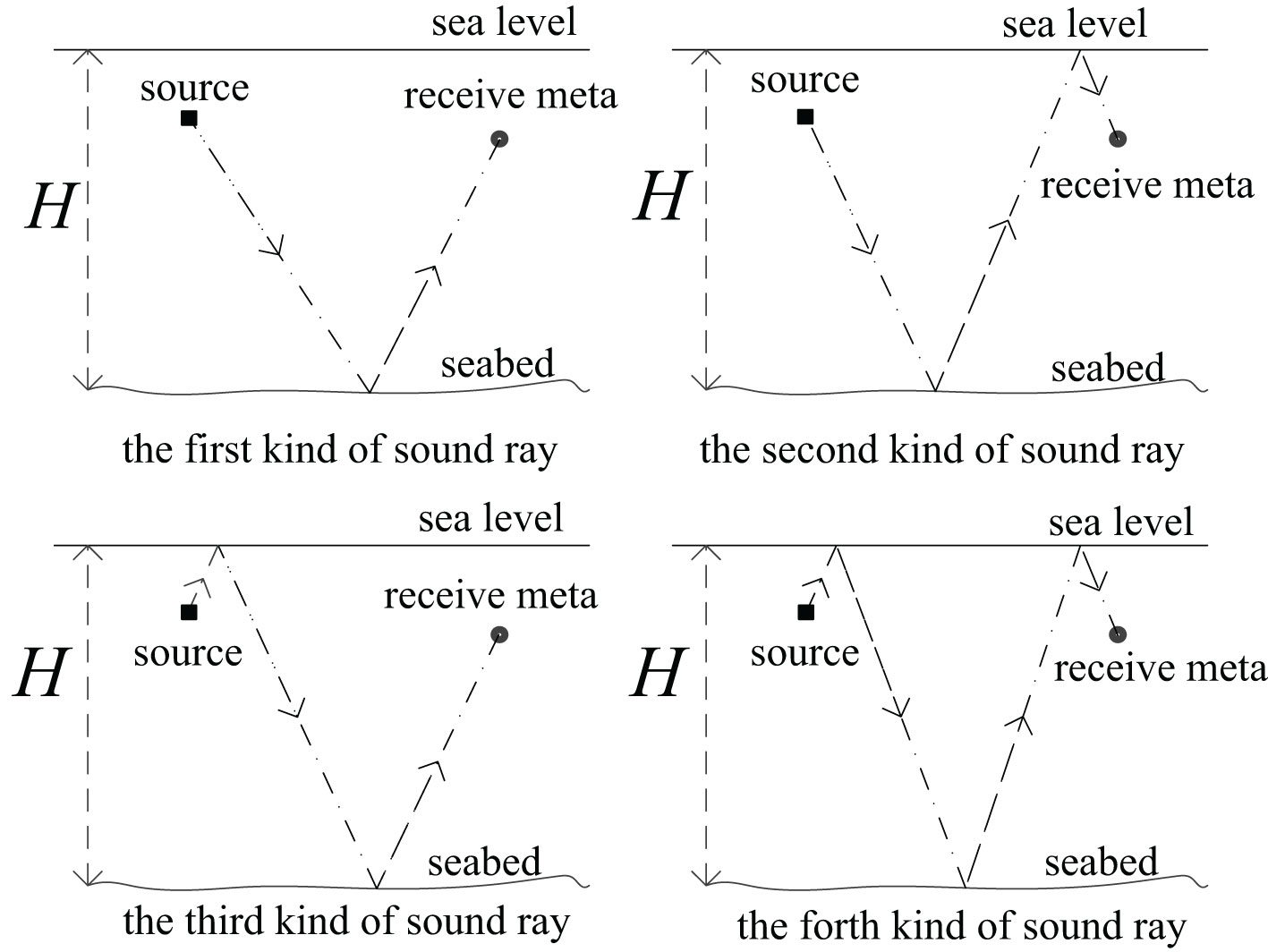
Figure 1 The four types of multipath sound rays contributing to the intensity of seafloor reverberation.

In this figure, H represents the depth of the sea. The paths of these four types of sound rays involve the following: a) sound source, scattering at the bottom surface, and hydrophone; b) sound source, scattering at the bottom surface, sea surface reflection, and hydrophone; c) sound source, sea surface reflection, scattering at the bottom surface, and hydrophone; d) sound source, sea surface reflection, scattering at the bottom surface, second sea surface reflection, and hydrophone.

In general, the combined transmitter and receiver can be regarded as a special case of a separated transmitter and receiver. Therefore, considering that the towed linear array sonar to be analyzed is a separated transmitter and receiver, the present study investigated the establishment of a sonar reverberation simulation model under the condition of a separated sound source and hydrophone.

2.2 Reverberation signal model considering the Doppler effect

The model in this paper is based on the following three hypotheses:

Hypothesis 1: Sound waves propagate in the form of spherical waves.

Hypothesis 2: The absorption of sound waves is neglected, and thus scattering is calculated at the sea bottom, and reflection is calculated at the sea surface.

Hypothesis 3: Scattering of the sea bottom is uniform.

The influence of the Doppler effect on sonar reverberation signal mainly affects signal frequency and signal pulse width.

2.2.1 Doppler effect on signal frequency

Let us consider a sinusoidal signal where the signal (Jian, 2019) source moves at a radial rate v relative to the hydrophone. Let the velocity of the sound source close to the hydrophone be positive and the velocity of the sound source far away from the hydrophone negative. If the frequency of the signal is f, the wavelength is λ, and the propagation speed of the signal in the medium is c, the frequency of the signal after the Doppler effect becomes f′, and the wavelength becomes λ′. Consequently (Xianwen et al., 2022), the Doppler shift is given by Δf = f′-f or

\begin{array}{l} Δ f = \frac{v}{c - v} \cdot f & (1) \end{array}

In the rectangular coordinate system, a sound source is assumed to be moving with a velocity v_t, the hydrophone moves with a velocity v_r, and the bottom scatterer dA is static, whereas all other environmental conditions remain unchanged. The Doppler shift models of four types of multipath sound rays are discussed respectively in the following.

2.2.1.1 Doppler shift model of the first type of sound ray

As shown in Figure 2-1, SS represents the sound source, RE is the receiving element, $r_{1}$ is the propagation vector of the first segment of the sound ray, and r₂ is the propagation vector of the second segment of the sound ray. Furthermore, φ is the scattering azimuth angle, θ^I is the grazing angle of the incident sound ray, θ^s is the grazing angle of the scattered sound ray, and n is a scattering element serial number (Sheng and Xucheng, 2010).

FIGURE 2

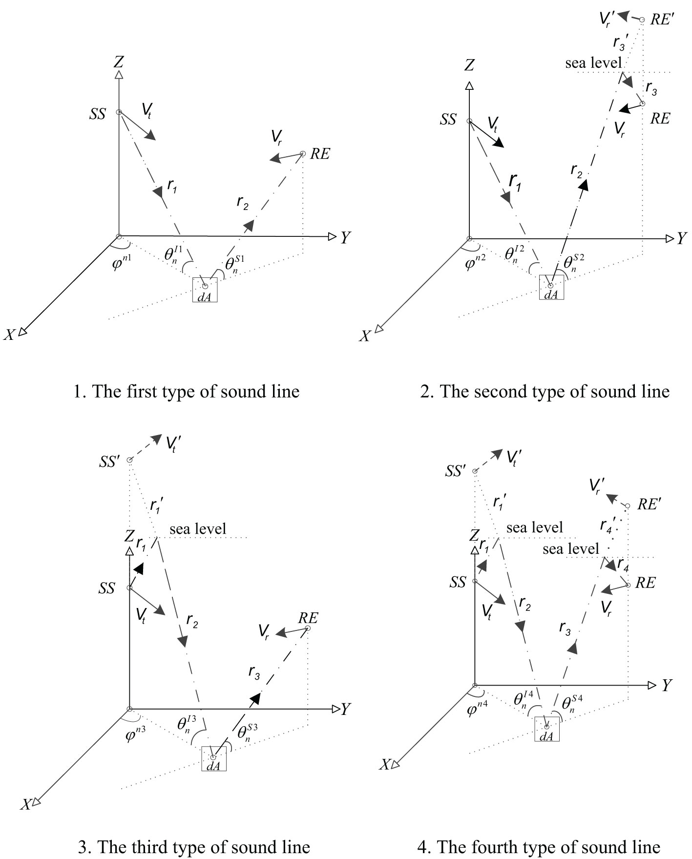
Figure 2 Four types of sound line.

First, we investigate the section of the first type of sound ray from the sound source SS to the bottom scatterer dA. Let the frequency shift of the signal received by the seafloor scatterer be Δf₁_t. In accordance with the physical meaning of the vector dot product, the radial velocity v_t on r₁ can be expressed as

\begin{array}{l} v_{1} = \frac{V_{t} \cdot r_{1}}{| r_{1} |} & (2) \end{array}

If we substitute the relevant parameters of the first type of sound ray into Equation (1), the variation of the signal frequency Δf₁_t of the first type of sound ray transmitted from the sound source to the scattering element dA can be obtained as follows (Zhongchen et al., 2013):

\begin{array}{l} Δ f_{1 t} = \frac{v_{1}}{c - v_{1}} \cdot f & (3) \end{array}

If we substitute Equation (2) into Equation (3), we can obtain the frequency shift of the sound source as it hits the seafloor scattering element via r₁:

\begin{array}{l} Δ f_{1 t} = \frac{V_{t} \cdot r_{1}}{c \cdot | r_{1} | - V_{t} \cdot r_{1}} \cdot f & (4) \end{array}

Similarly, considering the propagation of the first type of sound ray from the scattering element dA through r₂ to the hydrophone RE, we can assume that the frequency of the signal scattered by the first type of sound ray on the seabed is f₁_b.

Consequently, the relationship between f₁_b and the original frequency f of the signal is:

\begin{array}{l} f_{1 b} = f + Δ f_{1 t} & (5) \end{array}

Assuming that the velocity of the hydrophone is v_r, the frequency shift Δf_1r of the received signal for the first type of sound ray from the seafloor scatterer $d A$ to the hydrophone is

\begin{array}{l} Δ f_{1 r} = \frac{V_{r} \cdot r_{2}}{c \cdot | r_{2} | - V_{r} \cdot r_{2}} \cdot f_{1 b} & (6) \end{array}

and the total Doppler shift of the first type of sound ray is: (Yao, 2013)

\begin{array}{l} Δ f_{1} = Δ f_{1 t} + Δ f_{1 r} = [\frac{V_{t} \cdot r_{1}}{c \cdot | r_{1} | - V_{t} \cdot r_{1}} + \frac{V_{r} \cdot r_{2}}{c \cdot | r_{2} | - V_{r} \cdot r_{2}} \cdot (1 + \frac{V_{t} \cdot r_{1}}{c \cdot | r_{1} | - V_{t} \cdot r_{1}})] \cdot f & (7) \end{array}

According to formulas $(5 - 5)$ and $(5 - 13)$ in (Minghui, 2011), the first type of sound ray reverberation signal model $p_{1} (t_{1 k})$ can be obtained as (Yali, 2018):

\begin{array}{l} p_{1} (t_{1 k}) = \sum_{n = 1}^{N_{1}} \frac{1}{| r_{1} | \cdot | r_{2} |} \cdot s (t - t_{k}) \cdot \sqrt{\sin θ_{n}^{I 1} \sin θ_{n}^{S 1}} d A \cdot μ_{p}^{' n 1} \cdot \exp (j φ^{n 1}), & () \end{array}

where $s (t - t_{k})$ is the signal emitted by the sound source, and $s (t)$ passes through $t_{k}$ .

Considering the Doppler shift, after replacing $s (t - t_{k})$ with a complex signal $\exp [j 2 π (f + Δ f_{1}) (t - t_{1 k})]$ (Zhang et al., 2021a; Zhang et al., 2022a), we can get the first type of sound line reverberation signal model $p_{1} (t_{1 k})$ as:

\begin{array}{l} p_{1} (t_{1 k}) = \sum_{n = 1}^{N_{1}} \frac{1}{| r_{1} | \cdot | r_{2} |} \cdot \exp [j 2 π (f + Δ f_{1}) (t - t_{1 k})] \cdot \sqrt{\sin θ_{n}^{I 1} \sin θ_{n}^{S 1}} d A \cdot μ_{p}^{' n 1} \cdot \exp (j φ^{n 1}) & (8) \end{array}

where the first term ${(| r_{1} | \cdot | r_{2} |)}^{- 1}$ reflects the signal propagation loss; $r_{1}$ is the vector of sound sources to seafloor scattering elements; the second term $\exp [j 2 π (f + Δ f_{1}) (t - t_{1 k})]$ is the complex signal arriving at the hydrophone after the frequency shift and time delay; $f$ is the frequency of the transmitted signal; $Δ f_{1}$ is the total Doppler shift of the first type of sound; $t_{1 k} = (| r_{1} | + | r_{2} |) / c$ is the signal propagation time delay; and the third term $\sqrt{\sin θ_{n}^{I 1} \sin θ_{n}^{S 1}} d A \cdot μ_{p}^{' n 1} \cdot \exp (j φ^{n 1})$ is the scattering coefficient of the seabed sound pressure; $d A$ is the scattering element area; $μ_{p}^{' n 1}$ is a proportional constant, which is subject to the Gaussian distribution (Xiaohui et al., 2017); $φ^{n 1}$ is the transient phase, which is subject to the $(0 \sim 2 π)$ uniform distribution; n is the serial number of seabed scattering elements; $θ_{n}^{I 1}$ is the incidence grazing angle; $θ_{n}^{S 1}$ is the scattering grazing angle; $N_{1}$ is the total number of scattering elements.

Similarly, the three remaining types of sound ray Doppler shift models and reverberation signal models can be deduced accordingly.

2.2.1.2 The Doppler shift model of the second type of sound ray

As shown in Figure 2-2, the frequency change of the second type sound ray signal is given by the following equations:

\begin{array}{l} Δ f_{2 t} = \frac{V_{t} \cdot r_{1}}{c \cdot | r_{1} | - V_{t} \cdot r_{1}} \cdot f & (9) \end{array}

\begin{array}{l} Δ f_{2 r} = \frac{V_{r} \cdot (r_{2} + r_{3}^{'})}{c | r_{2} + r_{3}^{'} | - V_{r}^{'} \cdot (r_{2} + r_{3}^{'})} \cdot f_{2 b} & (10) \end{array}

where $V_{r}^{'}$ is the velocity of the virtual source RE′ of the hydrophone RE which is symmetrical to the sea surface, $r_{3}^{'}$ is the vector from the intersection of the scattered sound ray and the sea surface to the virtual source RE′, and r₃ is the propagation vector of the third segment of the sound ray, $f_{2 b} = f + Δ f_{2 t}$ .

The total Doppler shift of the second type of sound ray is

\begin{array}{l} Δ f_{2} = Δ f_{2 t} + Δ f_{2 r} = [\frac{V_{t} \cdot r_{1}}{c \cdot | r_{1} | - V_{t} \cdot r_{1}} + \frac{V_{r}^{'} \cdot (r_{2} + r_{3}^{'})}{c | r_{2} + r_{3}^{'} | - V_{r}^{'} \cdot (r_{2} + r_{3}^{'})} \cdot (1 + \frac{V_{t} \cdot r_{1}}{c \cdot | r_{1} | - V_{t} \cdot r_{1}})] \cdot f & (11) \end{array}

and the model of the second type of sound ray reverberation signal $p_{2} (t_{2 k})$ is

\begin{array}{l} p_{2} (t_{2 k}) = \sum_{n = 1}^{N_{1}} \frac{m}{| r_{1} | \cdot | r_{2} + r_{3}^{'} |} \cdot \exp [j 2 π (f + Δ f_{2}) (t - t_{2 k})] \cdot \sqrt{\sin θ_{n}^{I 2} \sin θ_{n}^{S 2}} d A \cdot μ_{p}^{' n 2} \cdot \exp (j φ^{n 2}) & (12) \end{array}

Here, the first term $m \cdot {(| r_{1} | \cdot | r_{2} + r_{3}^{'} |)}^{- 1}$ represents the signal propagation loss, the second term $\exp [j 2 π (f + Δ f_{2}) (t - t_{2 k})]$ is the complex signal arriving at the hydrophone after the frequency shift and time delay, and the third term $\sqrt{\sin θ_{n}^{I 2} \sin θ_{n}^{S 2}} d A \cdot μ_{p}^{' n 2} \cdot \exp (j φ^{n 2})$ is the sea bottom sound pressure scattering coefficient, m is the sea surface reflectivity, $μ_{p}^{' n 2}$ obeys a Gaussian distribution, $φ^{n 2}$ obeys a $(0 ~ 2 π)$ uniform distribution, and $t_{2 k} = (| r_{1} | + | r_{2} | + | r_{3} |) / c$ is the signal propagation delay.

2.2.1.3 The Doppler shift model of the third type of sound ray

As shown in Figure 2-3, the amount of change in the frequency of the third type of sound ray signal:

\begin{array}{l} Δ f_{3 t} = \frac{V_{t}^{'} \cdot (r_{1}^{'} + r_{2})}{c | r_{1}^{'} + r_{2} | - V_{t}^{'} \cdot (r_{1}^{'} + r_{2})} \cdot f & (13) \end{array}

\begin{array}{l} Δ f_{3 r} = \frac{V_{r} \cdot r_{3}}{c \cdot | r_{3} | - V_{r} \cdot r_{3}} \cdot f_{3 b} & (14) \end{array}

where $V_{t}^{'}$ is the velocity of the virtual source SS′, whose sound source SS is symmetrical to the sea surface, and $r_{3}^{'}$ is the vector from the intersection point of the incident sound ray and the sea surface to SS′, $f_{3 b} = f + Δ f_{3 t}$ .

The total Doppler shift of the third type of sound ray is:

\begin{array}{l} Δ f_{3} = Δ f_{3 t} + Δ f_{3 r} = [\frac{V_{t}^{'} \cdot (r_{1}^{'} + r_{2})}{c | r_{1}^{'} + r_{2} | - V_{t}^{'} \cdot (r_{1}^{'} + r_{2})} + \frac{V_{r} \cdot r_{3}}{c \cdot | r_{3} | - V_{r} \cdot r_{3}} \cdot (1 + \frac{V_{t}^{'} \cdot (r_{1}^{'} + r_{2})}{c | r_{1}^{'} + r_{2} | - V_{t}^{'} \cdot (r_{1}^{'} + r_{2})})] \cdot f & (15) \end{array}

and the model of the third type of sound ray reverberation signal $p_{3} (t_{3 k})$ is

\begin{array}{l} p_{3} (t_{3 k}) = \sum_{n = 1}^{N_{1}} \frac{m}{| r_{1}'^{} + r_{2} | \cdot | r_{3} |} \cdot \exp [j 2 π (f + Δ f_{3}) (t - t_{3 k})] \cdot \sqrt{\sin θ_{n}^{I 3} \sin θ_{n}^{S 3}} d A \cdot μ_{p}^{' n 3} \cdot \exp (j φ^{n 3}) & (16) \end{array}

The first term $m \cdot {(| r_{1} {^{'}}^{¢} + r_{2} | \cdot | r_{3} |)}^{- 1}$ represents the signal propagation loss, the second term $\exp [j 2 π (f + Δ f_{3}) (t - t_{3 k})]$ is the complex signal arriving at the hydrophone after the frequency shift and time delay, and the third term $\sqrt{\sin θ_{n}^{I 3} \sin θ_{n}^{S 3}} d A \cdot μ_{p}^{' n 3} \cdot \exp (j φ^{n 3})$ is the scattering coefficient of the seabed sound pressure, $μ_{p}^{' n 3}$ obeys a Gaussian distribution, $φ^{n 3}$ obeys a $(0 \sim 2 π)$ uniform distribution, and $t_{3 k} = (| r_{1} | + | r_{2} | + | r_{3} |) / c$ is the signal propagation delay.

2.2.1.4 Doppler shift model of the fourth type of sound ray

As shown in Figure 2-4, the amount of change in the frequency of the fourth type of sound ray signal is

\begin{array}{l} Δ f_{4 t} = \frac{V_{t}^{'} \cdot (r_{1}^{'} + r_{2})}{c | r_{1}^{'} + r_{2} | - V_{t}^{'} \cdot (r_{1}^{'} + r_{2})} \cdot f & (17) \end{array}

\begin{array}{l} Δ f_{4 r} = \frac{V_{r}^{'} \cdot (r_{3} + r_{4}^{'})}{c | r_{3} + r_{4}^{'} | - V_{r}^{'} \cdot (r_{3} + r_{4}^{'})} \cdot f_{4 b} & (18), \end{array}

where $r_{1}^{'}$ is the vector from the intersection point of the incident sound ray and the sea surface to SS’, r₄ is the propagation vector of the fourth segment of the sound ray, and $r_{4}^{'}$ is the vector from the intersection point of the scattered sound ray and the sea surface to the virtual source RE′, $f_{4 b} = f + Δ f_{4 t}$ .

Consequently, the total Doppler frequency shift of the fourth type of sound ray is (Zhang et al., 2021b):

\begin{array}{l} Δ f_{4} = Δ f_{4 t} + Δ f_{4 r} = [\frac{V_{t}^{'} \cdot (r_{1}^{'} + r_{2})}{c | r_{1}^{'} + r_{2} | - V_{t}^{'} \cdot (r_{1}^{'} + r_{2})} + \frac{V_{r}^{'} \cdot (r_{3} + r_{4}^{'})}{c | r_{3} + r_{4}^{'} | - V_{r}^{'} \cdot (r_{3} + r_{4}^{'})} \cdot (1 + \frac{V_{t}^{'} \cdot (r_{1}^{'} + r_{2})}{c | r_{1}^{'} + r_{2} | - V_{t}^{'} \cdot (r_{1}^{'} + r_{2})})] \cdot f & (19) \end{array}

and the model of the fourth type of sound ray reverberation signal $p_{4} (t_{4 k})$ is:

\begin{array}{l} p_{4} (t_{4 k}) = \sum_{n = 1}^{N_{1}} \frac{m^{2}}{| r_{1}^{'} + r_{2} | \cdot | r_{3} + r_{4}^{'} |} \cdot \exp [j 2 π (f + Δ f_{4}) (t - t_{4 k})] \cdot \sqrt{\sin θ_{n}^{I 4} \sin θ_{n}^{S 4}} d A \cdot μ_{p}^{' n 4} \cdot \exp (j φ^{n 4}) & (20) \end{array}

The first term of Equation 20 $m^{2} {(| r_{1}^{'} + r_{2} | \cdot | r_{3} + r_{4}^{'} |)}^{- 1}$ represents the signal propagation loss, the second term $\exp [j 2 π (f + Δ f_{4}) (t - t_{4 k})]$ is the complex signal arriving at the hydrophone after the frequency shift and time delay, and the third term $\sqrt{\sin θ_{n}^{I 4} \sin θ_{n}^{S 4}} d A \cdot μ_{p}^{' n 4} \cdot \exp (j φ^{n 4})$ is the scattering coefficient of the seabed sound pressure, $μ_{p}^{' n 4}$ obeys a Gaussian distribution, $φ^{n 4}$ obeys a $(0 \sim 2 π)$ uniform distribution, and $t_{4 k} = (| r_{1} | + | r_{2} | + | r_{3} | + | r_{4} |) / c$ is the signal propagation delay.

2.2.2 Influence of the Doppler effect on the signal pulse width

As shown in Figure 3, c is the signal speed, λ is the wavelength, τ is the pulse width, and k is the number of cycles, i.e., the signal contains k wavelengths. The signal will be affected by the Doppler stretching effect, and will thus have a new wavelength λ′ and a new pulse width τ′ (Xiye et al., 2009). According to the relationship between distance, speed, and time, we can easily obtain that:

FIGURE 3

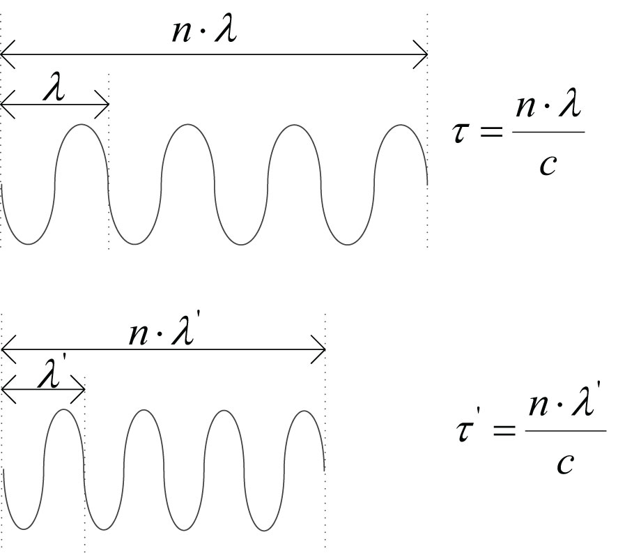
Figure 3 Influence of the Doppler stretching effect on the signal pulse width.

\begin{array}{l} τ = \frac{k \cdot λ}{c} & (21) \end{array}

\begin{array}{l} τ^{'} = \frac{k \cdot λ^{'}}{c} & (22) \end{array}

If we substitute $f \cdot λ = c$ and $f^{'} \cdot λ^{'} = c$ into Equation (21) and Equation (22), respectively, then we can obtain the relationship between the signal pulse width before and after the Doppler stretching effect:

\begin{array}{l} τ^{'} = \frac{f}{f^{'}} τ & (23) \end{array}

Simulation and results.

2.3 Underwater reverberation simulation

The geometric model of seabed reverberation simulation is shown in Figure 4 (Zhang and Yang, 2022). The towed linear array is horizontally arranged along the negative direction of the Y axis, where SS is the transmission source of the towed linear array located on the Z axis (Xiaohui et al., 2017). Furthermore, RE is the receiving element of the towed linear array, i is the serial number of the receiving element, N is the total number of receiving elements, d is the distance between the receiving elements, H is the depth of the sea water, and h is the distance of the towed linear array from the sea floor. The distance between the transmitting source SS and RE₁ is 2d (Jinhua et al., 2020; Yonghong, 2011). The motion states of the transmitting source and the receiving element are the same. The sea floor scattering area is an annular area, which assumes the origin as the center of a circle with an inner diameter $R_{\min}$ and an outer diameter $R_{\max}$ , and dA is a sea floor scattering element (Meina et al., 2017; Zhao et al., 2011). The transmitting source sends out a complex signal described by $s (t) = \exp (j 2 π f t)$ (Zhiguang and Zhiqiang, 2016), with a pulse width of τ, sea surface reflectivity of m, and speed c (Zhang et al., 2022b).

FIGURE 4

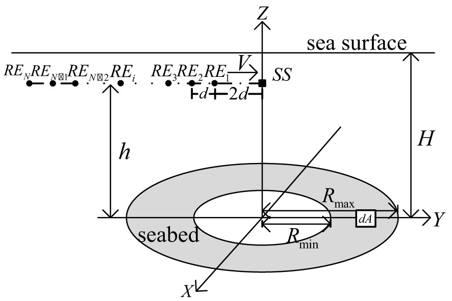
Figure 4 Geometric modeling of seabed reverberation simulation.

2.3.1 Reverberation signal simulation of a single scattering unit by a single sound source and a single hydrophone

In this section, we simulate the reverberation signal received by $R E_{1}$ , which is emitted by the sound source SS and is incident to $R E_{1}$ , via a single scattering element dA (Yuqiang et al., 2018). The simulation parameters are shown in the following Table 1:

TABLE 1

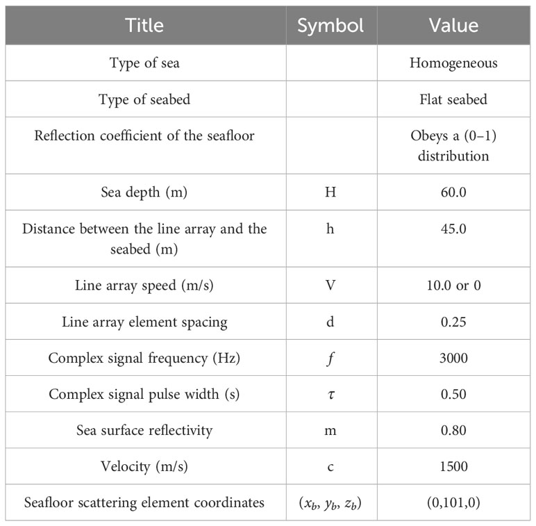
Table 1 Parameters used to simulate the single seafloor scattering element reverberation.

In this paper, the reverberation model, represented by Equations (24), (25), (26), and (27), takes into consideration both the ocean multipath and Doppler effect. Depending on whether the transmitting source and the single receiving element $R E_{1}$ are stationary or moving, the simulation results are shown in Figures 5, 6, respectively.

FIGURE 5

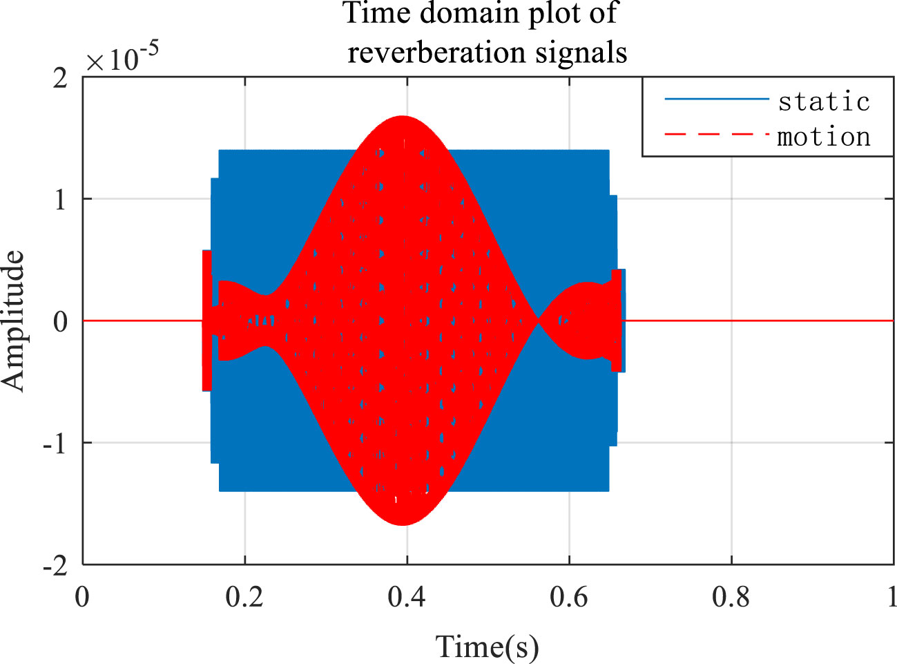
Figure 5 Time domain map of a single seafloor scattering element reverberation signal.

FIGURE 6

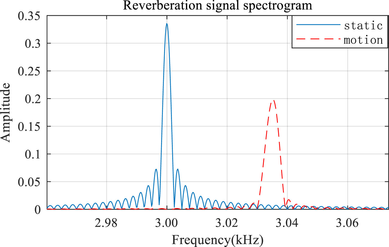
Figure 6 Spectrogram of a single seafloor scattering element reverberation signal.

Figure 5 demonstrates a time domain diagram of a single bottom scatterer’s reverberation signal. A single source emits a sinusoidal pulse signal with a fixed frequency pulse width of 0.5(s). After passing through the single scattering element $d A$ , the single hydrophone $R E_{1}$ , receives the time domain map of the signal. The blue part of the figure is the time domain plot of the signal received by $R E_{1}$ while the trailing linear array is stationary. Conversely, the red part of the figure is the time domain plot of the signal received by $R E_{1}$ when the linear array is dragged. Thus, when the transceiver device is stationary, the signal frequency of the four types of voice lines remains unchanged because there is no Doppler shift. Hence, the superimposed signal of the four types of voice lines still basically maintains the shape of sinusoidal pulses (blue part). When the transceiver device moves, the signals of the four types of voice lines undergo different degrees of Doppler shift. The superposition of four types of sound lines with different frequencies forms a signal (red part), in which the envelope amplitude changes following the law of sine and cosine. Moreover, under the same motion state, the Doppler frequency shift of the four types of voice lines is calculated by the Doppler shift model of the four types of voice lines, and the accurate modeling and simulation of sonar reverberation signals are realized. Additionally, owing to the influence of the Doppler effect on the signal pulse width, the signal pulse width of the light-colored part of the figure is shortened, and the analysis graph shows the pulse width change $Δ τ = τ^{'} - τ = - 0.005$ (s).

In addition, Figure 6 exhibits a spectrum diagram of the reverberation signal generated by a single bottom scatterer (Yanzi et al., 2018). It can be seen that the peak center of the spectrum increases following the movement of the transceiver, as opposed to when the transceiver remains stationary, and the analysis graph demonstrates that the frequency shift is $Δ f = 35$ Hz (Huang and Gao, 2014). When in motion, the spectrum is extended due to the different Doppler frequency shifts of the four types of sound rays moving at the same speed.

Although (Minghui, 2011) provides the models of four types of multipath sound ray reverberation signals, the authors do not investigate the influence of the Doppler effect on the four types of sound ray reverberation signals in detail. To compare the traditional model, which does not consider the multipath and the Doppler effect, with the improved model presented in this paper, we employed the first type of bistatic sound ray model equations $(5 - 12)$ stated in Chapter 5 of (Minghui, 2011) to compare the simulation results with the present model.

In the case of motion, Figure 7 shows a comparison of the simulation time domain of a single seafloor scatterer:

FIGURE 7

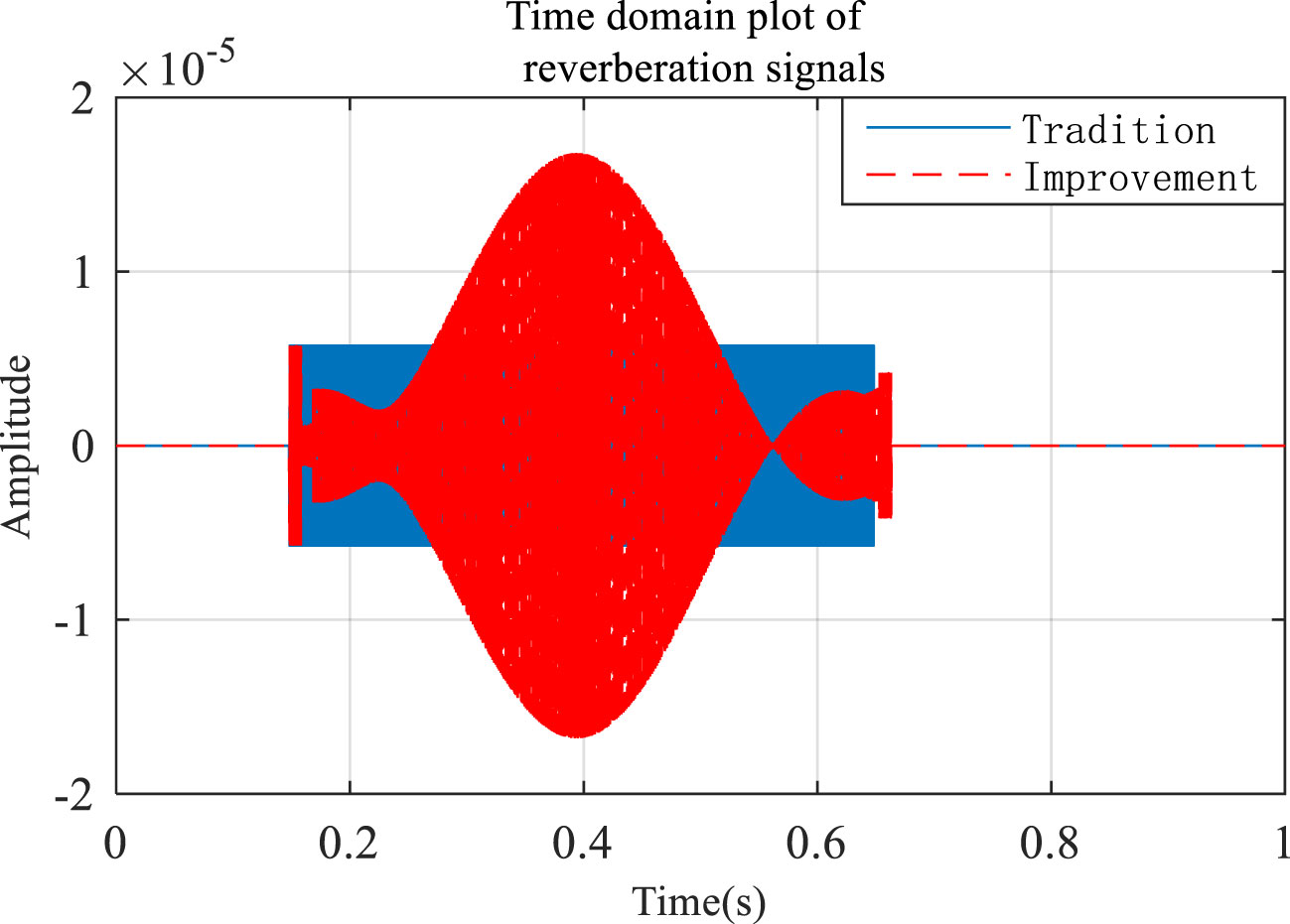
Figure 7 Comparison of the time domain diagram of a single seafloor scattering element reverberation signal.

The blue graph in Figure 7 is a time domain plot of the received signal simulated based on a traditional model. Conversely, the red graph is a time domain plot of the received signal simulated using the improved model. Figure 7 reveals that the time domain of the reverberation signals of the improved and traditional models is as follows: 1. The pulse width of the improved model signal is longer than that of the traditional model signal, which is due to the influence of the multipath, and part of the sound ray propagation path is longer. Since the Doppler frequency shift is not considered by the traditional model, the reverberation amplitude will remain constant. Compared with the traditional model, the reverberation envelope of the improved model changes according to the sine and cosine law, which is due to the superposition of reverberation signals formed by the different Doppler shifts of the four types of sound rays. The reverberation time domain amplitude of the traditional model is smaller than the signal amplitude under static conditions in Figure 5 because the traditional first type of sound ray model does not consider multipath superposition. It can be seen that the improved model can reflect the space-time characteristics of reverberation signals more accurately in the case of a single source, single hydrophone, and single scatterer.

The frequency domain comparison between the improved model and the traditional model is shown in Figure 8:

FIGURE 8

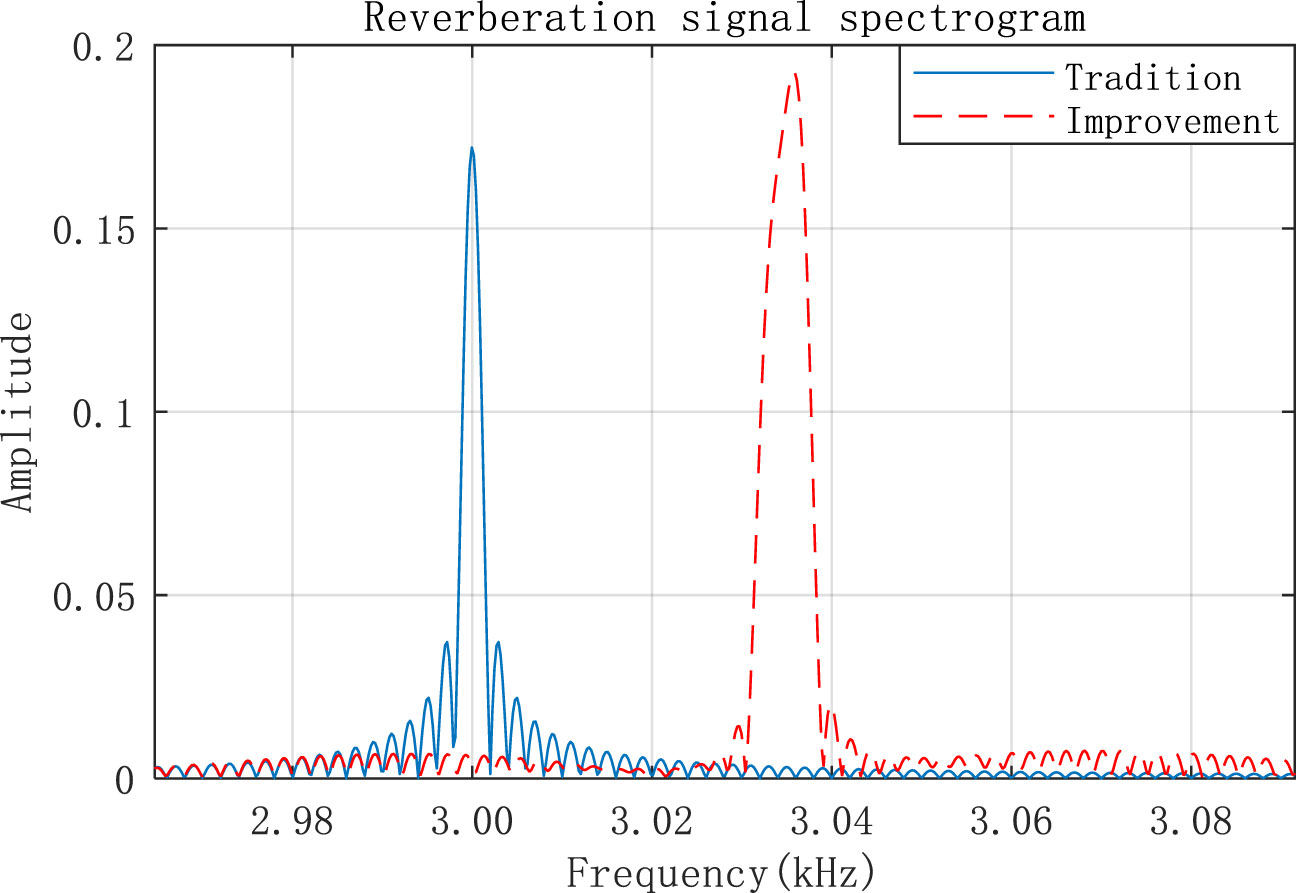
Figure 8 Frequency domain comparison diagram of a single seafloor scattering element reverberation signal.

From Figure 8, we can see that the peak frequency of the improved model increases due to the influence of the Doppler shift, and the spectrum of the improved model is extended compared with the traditional model because of the different Doppler frequency shifts of different sound rays caused by the ocean multipath. Therefore, the improved model can reflect the spectrum characteristics of the reverberation signal more accurately. In addition, the improved model presented in this study can simulate the reverberation signal more accurately under the condition of a single source, single hydrophone, and single scattering unit by analyzing the respective space-time and spectrum characteristics.

2.3.2 Reverberation signal simulation of a towed linear array

In this section, we simulate the reverberation signal of a towed linear array using the parameters shown in Table 2 and the simulation results are shown in Figures 9–12.

TABLE 2

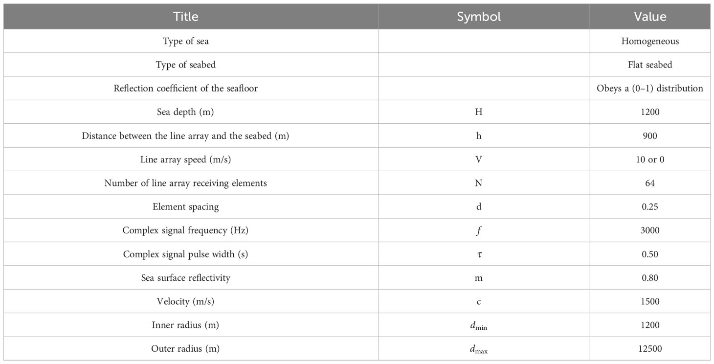
Table 2 Dragging line array reverberation simulation parameters.

FIGURE 9

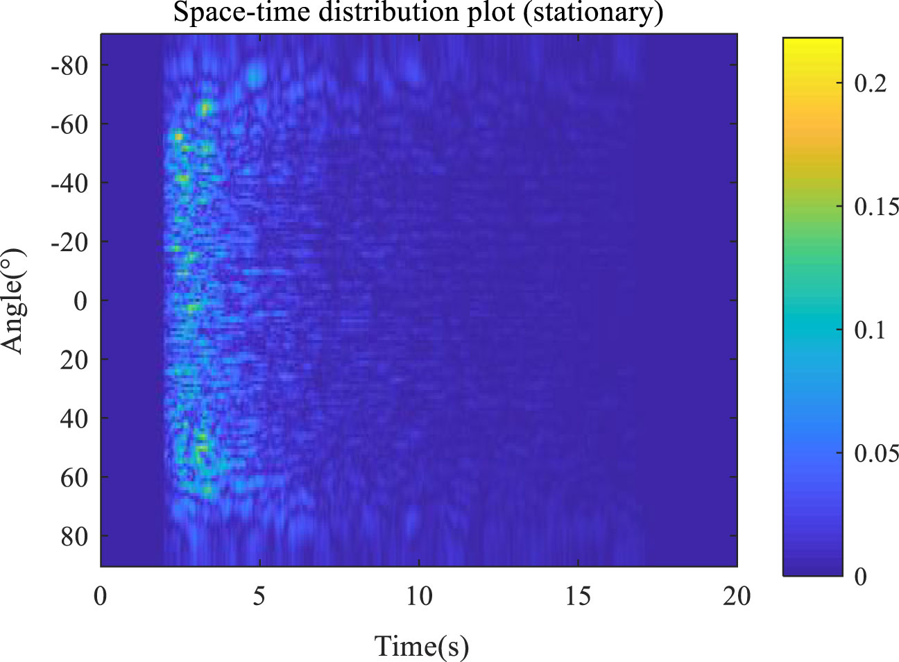
Figure 9 Space-time distribution of a stationary dragging line array reverberation signal.

FIGURE 10

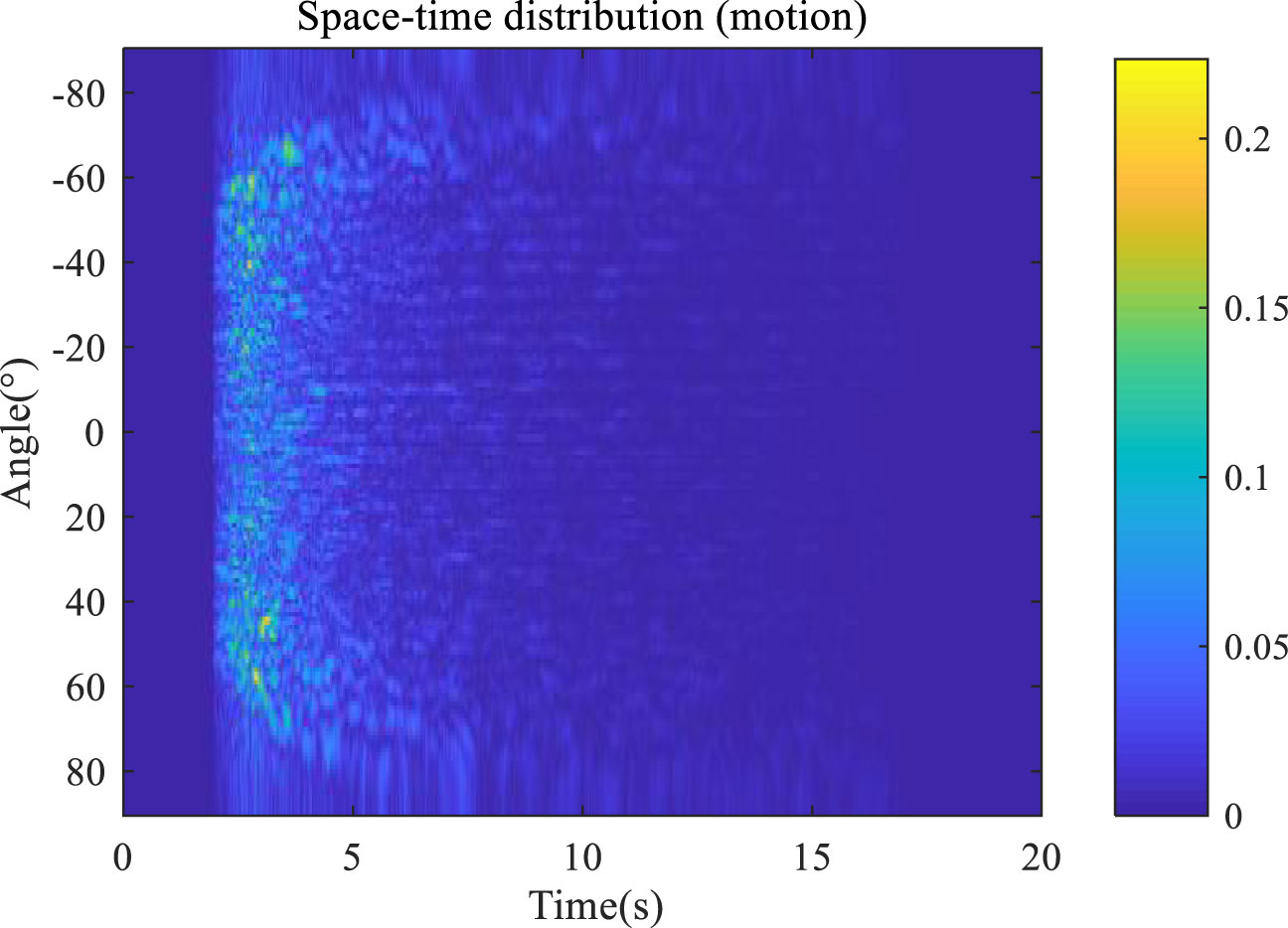
Figure 10 Space-time distribution of a panned dragging line array reverberation signal.

FIGURE 11

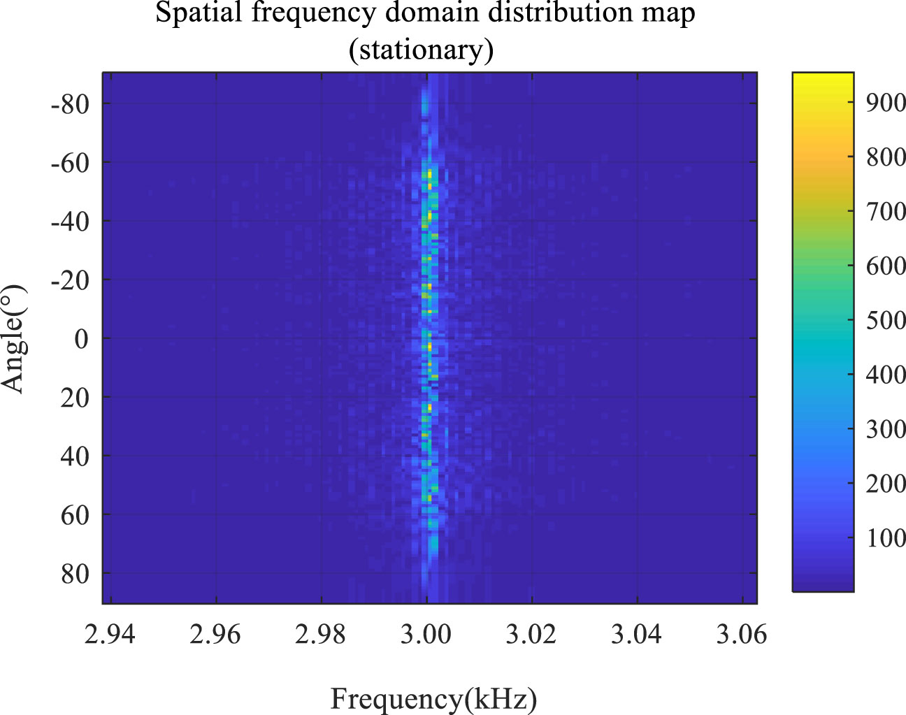
Figure 11 Space-frequency distribution of a stationary dragging line array reverberation signal.

FIGURE 12

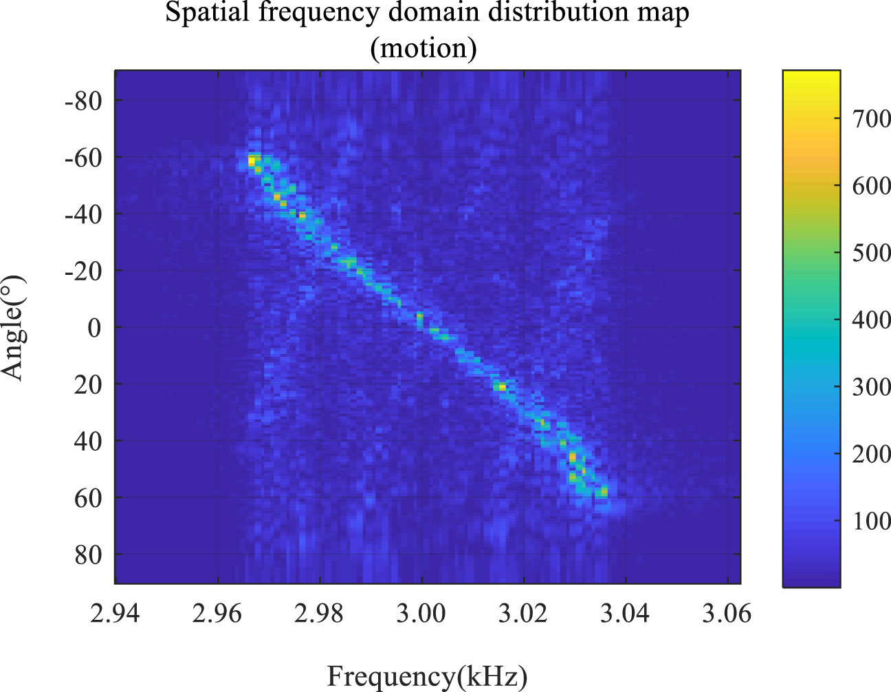
Figure 12 Space-frequency distribution of a panned dragging line array reverberation signal.

The “angle” in Figures 9–12 describes the directivity angle of the dragged line array (Zhe et al., 2017; Zelin, 2019; Junchao, 2021). Furthermore, different angles correspond to scattering elements at different positions. A comparison between Figures 11, 12 demonstrates that the reverberation signal frequency decreases when the directivity angle is negative, and increases when the directivity angle is positive. Figure 12 also shows that the frequency shift of the reverberation signal is approximately sinusoidal with the directivity angle of the linear array, a finding which is consistent with the theoretical analysis (Xiaodong et al., 2011; Yanqiu, 2015; Zhu et al., 2023; Zhang et al., 2023a; Zhang et al., 2023b).

Figures 13, 14 show the reverberation signal simulation of the traditional model under the condition of towed linear array motion

FIGURE 13

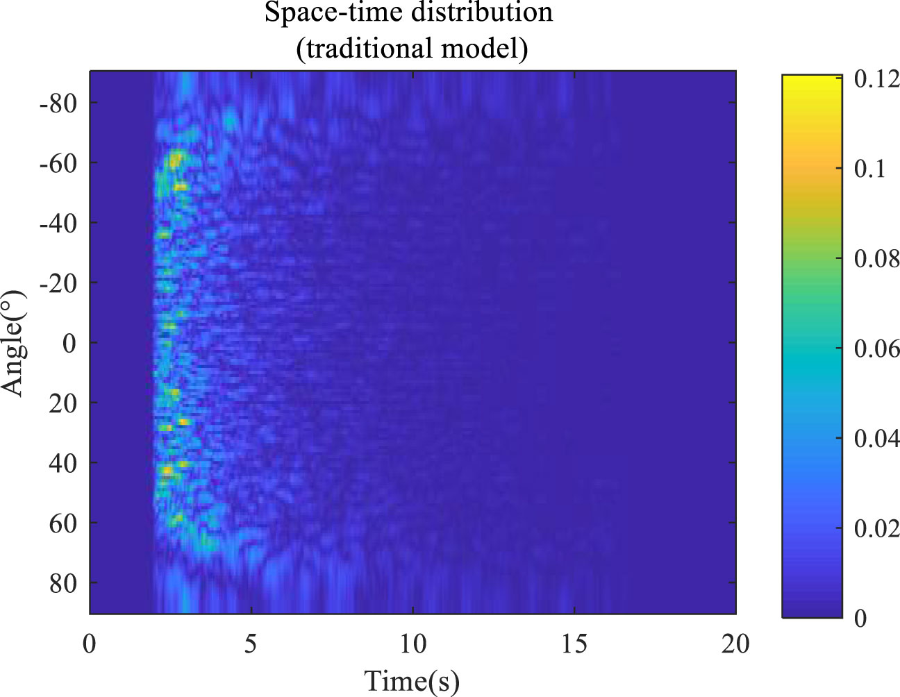
Figure 13 Space-time distribution of a panned dragging line array traditional model reverberation signal.

FIGURE 14

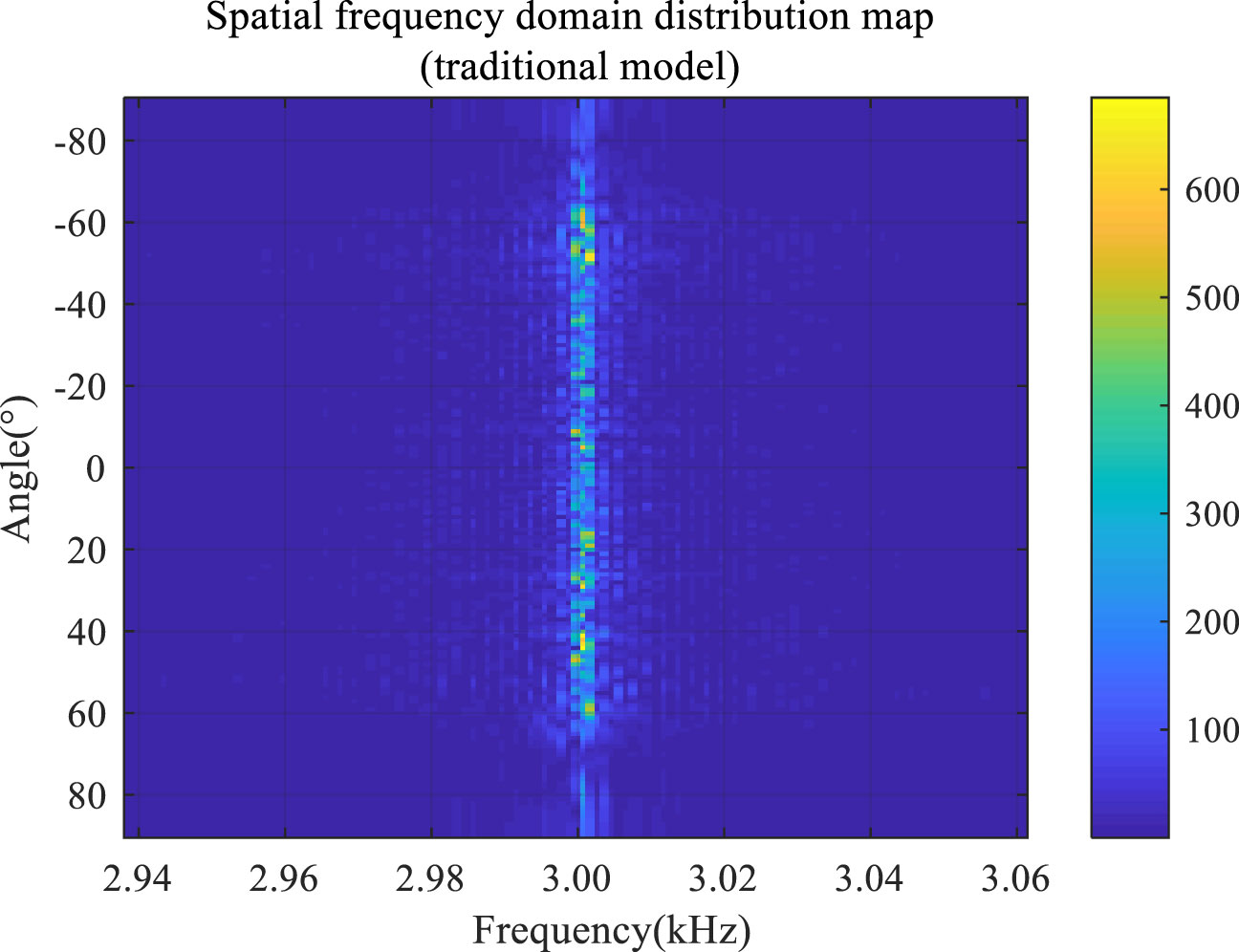
Figure 14 Space-frequency distribution of a panned dragging line array traditional model reverberation signal.

A comparison between Figures 13 and 10 reveals that the maximum amplitude of the reverberation signal of the traditional model is 0.12, which is smaller than the maximum amplitude of the reverberation signal of the improved model (0.22). This improvement can be explained by the fact that the improved model considers the superposition of multipath sound rays. Furthermore, a comparison between Figures 14 and 12 demonstrates that potential changes in the directivity angle of the linear array do not induce any frequency shift in the reverberation signal of the traditional model. This is because the traditional model does not consider the Doppler frequency shift factor.

Overall, our findings clearly show that the improved model presented in this study can simulate the reverberation signal significantly more accurately compared to the traditional models by analyzing space-time and spectral characteristics under the condition of a towed linear array.

3 Conclusion and discussion

Under the condition of a single sound source, single hydrophone, and single scattering unit, our simulation data showed that the envelope amplitude of the reverberation signal changes according to the sine and cosine law, while changes in the pulse width and spectrum of the signal will occur when the transceiver moves in response to the Doppler effect. A comparison between the simulation results of the improved and the traditional models clearly demonstrates that the reverberation pulse width of the improved model is longer than that of the traditional model due to the ocean multipath. In addition, the reverberation envelope of the improvement model changes according to the sine and cosine law, caused by the superposition of reverberation signals formed by the different Doppler frequency shifts of the four types of sound rays considered, as opposed to the reverberation signal amplitude of the traditional model which remains unchanged. When assessing the space-frequency characteristics of the two models, the peak frequency of the improved model was increased and the spectrum width was extended due to the different Doppler frequency shift of the multipath sound ray. It can also be seen that the reverberation signal model that considers both the ocean multipath and the Doppler effect can reflect the variation in the frequency and pulse width of the reverberation signal far more accurately.

Under the condition of a towed linear array, the relationship between the frequency shift of the reverberation signal and the directivity angle of the linear array is approximately sinusoidal when the linear array is in uniform linear motion, and the space-time two-dimensional characteristics and Doppler spread in the simulation results are consistent with the theoretical analysis. Our findings confirm that the model established on the premise of single-point transceiver separation can be well-extended to the case of multi-point separation. Consequently, the proposed model has broad universal applicability and can be used to simulate more diverse combinations of sonar array elements.

When it comes to space-time characteristics, our data showed that the reverberation amplitude of the improved model is larger than that of the traditional model due to the superposition of multipath sound rays in the ocean. Finally, pertaining to the spatial frequency characteristics, the improved model can reflect the frequency domain characteristics of reverberation signals more accurately than the traditional model.

Conclusively, the reverberation signal model considering both the ocean multipath and the Doppler effect can simulate the sonar reverberation signal more accurately than the traditional models presented in current literature.

Data availability statement

The original contributions presented in the study are included in the article/supplementary material. Further inquiries can be directed to the corresponding author.

Author contributions

SZ: Conceptualization, Data curation, Formal Analysis, Methodology, Software, Validation, Writing – original draft, Writing – review & editing. JW: Conceptualization, Formal Analysis, Investigation, Methodology, Writing – original draft, Writing – review & editing. TY: Writing – review & editing.

Funding

The authors declare financial support was received for the research, authorship, and/or publication of this article. This work was supported by the National Natural Science Foundation of China (NO.41976177).

Conflict of interest

The authors declare that the research was conducted in the absence of any commercial or financial relationships that could be construed as a potential conflict of interest.

Publisher’s note

All claims expressed in this article are solely those of the authors and do not necessarily represent those of their affiliated organizations, or those of the publisher, the editors and the reviewers. Any product that may be evaluated in this article, or claim that may be made by its manufacturer, is not guaranteed or endorsed by the publisher.

References

Bing J., Yunfei C., Yang Z., Rui W. (2016). Analysis of ocean reverberation characteristics based on the vector hydrophones. Tech. Acoustics 35 (3), 110–114.

Google Scholar

Danping S. (2020). Modeling and simulation of seabed reverberation in shallow seas. Aud Eng. 44, 31–32,36. doi: 10.16311/j.audioe.2020.08.008

CrossRef Full Text | Google Scholar

Huang X., Gao T. (2014). Reverberation spectra modeling and simulation of arbitrary sea bottom shape. J. Syst. Simul 26, 2576–2580.

Google Scholar

Jian L. (2019). Interception detection and parameter estimation based on time-frequency image of underwater acoustic pulse signal (China: Southeast University).

Google Scholar

Jincheng Z. (2019). Research and implement on robust beamforming algorithm based on towed array (China: Harbin Engineering University).

Google Scholar

Jinhua L., Jinsong T., Haoran W. (2020). A MSR based range Doppler algorithm for the moderate squint multi-aperture synthetic aperture sonar. Tech. Acoustics 39(3), 354–359. doi: 10.16300/j.cnki.1000-3630.2020.03.017

CrossRef Full Text | Google Scholar

Jun F., Weilin T., Linkai Z. (2012). Planar elements method for forecasting the echo characteristics from sonar targets. J. Ship Mechanics 16 (1-2), 171–180.

Google Scholar

Junchao W. (2021). Research on self-noise suppression method of autonomous underwater vehicle (China: Zhejiang University).

Google Scholar

Kou S., Feng X. A., Bi Y., Huang H. (2021). High-resolution angle-Doppler imaging by sparse recovery of underwater acoustic signals. Chin. J. Acoustics 46, 519–528. doi: 10.15949/j.cnki.0371-0025.2021.04.004

CrossRef Full Text | Google Scholar

Lijun Y., Jinrong W. U., Shengming G., Zhang J., Hou Q., Ma L. (2021). Modeling and analysis of reverberation intensity in incomplete SOFAR channel. J. Harbin Eng. Univ 42, 325–330. doi: 10.11990/jheu.201912045

CrossRef Full Text | Google Scholar

Liya X. U. (2018). Researches on the method of geoacoustic inversion with bottom parameters in deep ocean (China: Northwestern Polytechnical University).

Google Scholar

Meina W., Gang B., Chao S., Wang W. (2017). Simulation analysis of vertically divided seafloor reverberation signal in ocean bathymetry. Hydrogr Surv Charting 37, 75–78. doi: 10.3969/j.issn.1671-3044.2017.01.019

CrossRef Full Text | Google Scholar

Minghui Z. (2011). Research on bottom sound scattering strength measurement method and reverberation properties in irregular sea area (China: Harbin Engineering University).

Google Scholar

Runze X., Rui D., Kunde Y., Ma Y., Guo Y. (2021). Modeling and analysis of monostatic incoherent boundary reverberation intensity in deep water. Acta Acust 46, 926–938. doi: 10.15949/j.cnki.0371-0025.2021.06.014

CrossRef Full Text | Google Scholar

Sheng L., Xucheng C. (2010). Simulation research on reverberation for bistatic sonar system. Tech Acoust 29, 355–360. doi: 10.3969/j.issn1000-3630.2010.04.001

CrossRef Full Text | Google Scholar

Sibo L., Song L. (2016). A modeling and simulation based on K-distribution model. Ship Sci. Technol. 38, 158–161. doi: 10.3404/j.issn.1672-7619.2016.S1.029

CrossRef Full Text | Google Scholar

Sibo L. I. (2018). The characteristics of transceiver separation reverberation in shallow water (China: Harbin Engineering University).

Google Scholar

Tao H. (2007). The study on visual simulation techniques of underwater target (China: Harbin Engineering University).

Google Scholar

Teng Z., Chunhua Z., Peng W. (2021). Three-dimensional imaging sonar echo modeling simulation and analysis. Netw. New Media Technol. 10, 22–29.

Google Scholar

Xianwen Z., Zhou C., Zhengwei W., Zhigang L., Pengpeng H., Mengxin W. (2022). Echo signal modeling and simulation for moving target in complex marine environment. Mobile Commun. 46 (7), 82–87. doi: 10.3969/j.issn.1006-1010.2022.07.015

CrossRef Full Text | Google Scholar

Xiaodong C., Jianguo H., Qunfei Z. (2011). Modeling and simulation of spacetime reverberation for active sonar array. Comput. Simul 28, 365–368.

Google Scholar

Xiaohui H., Gang L., Cheng W., Chen W. (2017). Multi-beam bathymetry seabed reverberation simulation study. Hydrogr Surv Charting 37, 22–25. doi: 10.3969/j.issn.1671-3044.2017.01.006

CrossRef Full Text | Google Scholar

Xiye G., Shaojing S., Yueke W. (2009). Research on modeling and simulating seafloor reverberation with the moving sonar. J. Natl. Univ Def Technol. 31, 92–96.

Google Scholar

Yali S. (2018). Reverberation signal simulation and inhibition technology of reverberation based on multistatic sonar (China: Harbin Engineering University).

Google Scholar

Yangang H., Zhenhua Z., Hanfen L. I. (2020). Modeling technology for active sonar target echo signal. Command Inf Syst. Technol. 11, 70–75. doi: 10.3969/j.issn.1671-3044.2017.01.006

CrossRef Full Text | Google Scholar

Yanqiu Z. (2015). Simulation and research of underwater target acoustic imaging (China: Southeast University).

Google Scholar

Yanzi G., Guoliang L., Fusheng Z. (2018). Research on an engineering simulation model of ocean reverberation. Ship Electron Eng. 38, 123–125. doi: 10.3969/j.issn.1672-9730.2018.10.030

CrossRef Full Text | Google Scholar

Yao Z. (2013). Research on methods of active sonar target detection in shallow water condition (China: Harbin Engineering University).

Google Scholar

Yonghong Y. (2011). Research on multi-beam synthetic aperture sonar imaging technology (China: Harbin Engineering University).

Google Scholar

Yuliang H. (2020). Research on target echo detection technology of active sonar for small and moving platform (China: Harbin Engineering University).

Google Scholar

Yulu C., Xiaogang Y., Tuo Z. (2017). Numerical compute about near distance bottom reverberation of typical sound speed profiles in shallow sea. Ship Sci. Technol. 39, 94–97. doi: 10.3404/j.issn.1672-7619.2017.06.019

CrossRef Full Text | Google Scholar

Yuqiang L., Yan X., Shengzeng Z. (2018). Analysis of characteristics and research of modeling simulation on marine reverberation. Ship Electron Eng. 38, 86–88. doi: 10.3969/j.issn.1672-9730.2018.11.022

CrossRef Full Text | Google Scholar

Zelin S. (2019). Research of highlight feature extraction and recognition based on time-frequency domain filtering (China: Harbin Engineering University).

Google Scholar

Zhang X., Wu H., Sun H., Ying W. (2021a). Multireceiver SAS imagery based on monostatic conversion. IEEE J. Sel Top. Appl. Earth Obs Remote Sens. 14, 10835–10853. doi: 10.1109/JSTARS.2021.3121405

CrossRef Full Text | Google Scholar

Zhang X., Yang P. (2022). Back projection algorithm for multi-receiver synthetic aperture sonar based on two interpolators. J. Mar. Sci. Eng. 10, 718. doi: 10.3390/jmse10060718

CrossRef Full Text | Google Scholar

Zhang X., Yang P., Huang P., Sun H., Ying W. (2022a). Wide-bandwidth signal-based multireceiver SAS imagery using extended chirp scaling algorithm. IET Radar Sonar Navig 16, 531–541. doi: 10.1049/rsn2.12200

CrossRef Full Text | Google Scholar

Zhang X., Yang P., Sun H. (2022b). Frequency-domain multireceiver synthetic aperture sonar imagery with Chebyshev polynomials. Electron Lett. 58, 995–998. doi: 10.1049/ell2.12513

CrossRef Full Text | Google Scholar

Zhang X., Yang P., Sun M. (2023a). An omega-k algorithm for multireceiver synthetic aperture sonar. Electron Lett. 59, 1–3. doi: 10.1049/ell2.12859

CrossRef Full Text | Google Scholar

Zhang X., Yang P., Zhou M. (2023b). Multireceiver SAS imagery with generalized PCA. IEEE Geosci Remote Sens Lett. 20, 1502205. doi: 10.1109/LGRS.2023.3286180

CrossRef Full Text | Google Scholar

Zhang X., Ying W., Liu Y., et al. (2021b). “Processing multireceiver SAS data based on the PTRS linearization,” in IEEE international geoscience and remote sensing symposium, 11-16 July 2021, Brussels, Belgium. 167–517 (IEEE: Brussels, Belgium). doi: 10.1109/IGARSS47720.2021.9553688

CrossRef Full Text | Google Scholar

Zhao Y., Xian F., Yufeng Z., Wang Q. (2011). Simulation and space-time model of seafloor reverberation. Comput. Simul 12, 398–401.

Google Scholar

Zhe C., Zhizhong L., Xin G., Qijun L. (2017). Simulation of sonar target tracking and locating based on pressure hydrophone in ocean. Comput. simulation 34 (5), 1–6.

Google Scholar

Zhiguang X., Zhiqiang L. (2016). Analysis of small target sonar detective performance based on LFM signal. Audio Engi-neering 40 (4), 48–50. doi: 10.16311/j.audioe.2016.04.11

CrossRef Full Text | Google Scholar

Zhongchen D., Ya-an L., Yanfeng J. (2013). Shallow seafloor reverberation modeling and simulation of torpedo. Torpedo Technol. 21, 100–104.

Google Scholar

Zhou Y., Li Q., Li P., Gong J., Yang R. (2020). Active sonar signal modeling and simulation. Electron Opt Control 27, 14–17. doi: 10.3969/j.issn.1671-637X.2020.02.004

CrossRef Full Text | Google Scholar

Zhu J., Song Y., Jiang N., Xie Z., Fan C., Huang X. (2023). Enhanced Doppler resolution and sidelobe suppression performance for Golay complementary waveforms. Remote Sens 15, 2452. doi: 10.3390/rs15092452

CrossRef Full Text | Google Scholar

Keywords: reverberation, ray acoustics, ocean multipath, bottom scattering, Doppler, accurate modeling, signal simulation, towed linear array

Citation: Zhang S, Wu J and Yin T (2023) Simulation of sonar reverberation signal considering the ocean multipath and Doppler effect. Front. Mar. Sci. 10:1279693. doi: 10.3389/fmars.2023.1279693

Received: 18 August 2023; Accepted: 13 September 2023;
Published: 17 October 2023.

Edited by:

Xuebo Zhang, Northwest Normal University, China

Reviewed by:

Li Dawei, Naval Aviation University, China
Hanhao Zhu, Zhejiang Ocean University, China

Copyright © 2023 Zhang, Wu and Yin. This is an open-access article distributed under the terms of the Creative Commons Attribution License (CC BY). The use, distribution or reproduction in other forums is permitted, provided the original author(s) and the copyright owner(s) are credited and that the original publication in this journal is cited, in accordance with accepted academic practice. No use, distribution or reproduction is permitted which does not comply with these terms.

*Correspondence: Sen Zhang, johnson_xh@sina.com

Disclaimer: All claims expressed in this article are solely those of the authors and do not necessarily represent those of their affiliated organizations, or those of the publisher, the editors and the reviewers. Any product that may be evaluated in this article or claim that may be made by its manufacturer is not guaranteed or endorsed by the publisher.