Hydrographical implications of ship-induced turbulence in stratified waters, studied through field observations and CFD modelling

Ship-related energy pollution has received increasing attention but almost exclusively regarding radiated underwater noise, while the effect of ship-induced turbulence is lacking in the literature. Here we present novel results regarding turbulent wake development, the interaction between ship-induced turbulence and stratification, and discuss the impact of turbulent ship wakes in the surface ocean, in areas with intense ship traffic. The turbulent wake development was studied in situ, using Acoustic Doppler Current Profilers (ADCP) and conductivity, temperature, depth (CTD) observations of stratification, and through computational fluid dynamics (CFD) modelling. Our results show that the turbulent wake interacts with natural hydrography by entraining water from below the pycnocline, and that stratification influences the turbulent wake development by dampening the vertical extent, resulting in the wake water spreading out along the pycnocline rather than at the surface. The depth and intensity of the turbulent wake represent an unnatural occurrence of turbulence in the surface ocean. The ship-induced turbulence can impact local hydrography, nutrient dynamics and increase plankton mortality due to physical disturbance, especially in areas with intense traffic. Therefore, sampling and modelling of e.g., contaminants in shipping lanes need to consider hydrographic conditions, as stratification may alter the depth and spread of the wake, which in turn governs dilution. Finally, the frequent ship traffic in estuarine and coastal areas, calls for consideration of ship-induced turbulence when studying hydrographic processes.

1 Introduction

Anthropogenic introduction of energy to the marine environment is considered a type of pollution (MSFD, 2008/56/EC). Until now, energy pollution has mainly embraced studies on underwater noise, where ships are a well-recognised source (Duarte et al., 2021), and ship-induced waves inducing resuspension and erosion, (Soomere and Kask, 2003; Soomere, 2005; Kelpšaite et al., 2009), especially in areas with intense ship traffic. An additional type of energy pollution is ship-induced turbulence (Figure 1), pioneered by Jürgensen (1991) but still commonly overlooked. Nylund et al. (2021) advanced the characterisation and understanding of turbulent ship wakes from an environmental impact perspective through a combination of in situ and ex situ observations. Nylund et al. (2021) also estimated that the input of ship-induced turbulent energy can be in the same order of magnitude as natural wind-induced turbulence, in areas of intense ship traffic. Hence, there is a need to investigate the potential impacts of shipping on local/regional hydrography, especially in areas and seasons of natural stratification of the surface ocean.

Figure 1

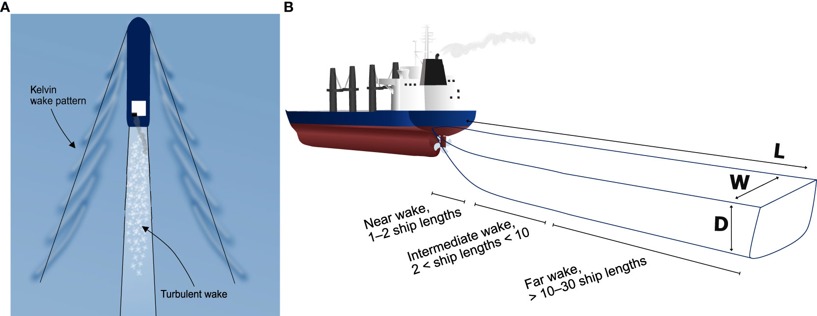
Figure 1 The turbulent wake region and the Kelvin wake pattern are illustrated in (A). The dimensionless length scales of the near field, intermediate, and far field wake regions are indicated in (B). L, wake longevity (in time or length); W, wake width, and D, wake depth. Note that these illustrations are schematics and not true in scale or shape. Figure reprinted with permission from Nylund (2023).

The development of the turbulent wake is affected by the ship’s speed, geometry, and manoeuvring, as well as environmental conditions such as currents, stratification, and waves (Loehr et al., 2001; Stanic et al., 2009; Ermakov and Kapustin, 2010; Voropayev et al., 2012; Fujimura et al., 2016; Somero et al., 2018). There are a dozen of studies where field observations of the wake extent have been presented with reported wake depths of 15–30 m, wake longevities of 10–20 min, and visible temperature signals in the surface water from ship-induced vertical mixing extending tens of kilometres after ship passage (Nylund et al. (2021) and references therein). None of studies reviewed by Nylund et al. (2021) investigated the turbulent wake. Instead, parameters such as the induced bubble cloud, temperature, or dilution of a dye/substance, were used as proxies for the turbulent wake extent. Regarding turbulent intensities, Nylund et al. (2021) calculated the rate of turbulent kinetic energy dissipation (ε) in the wake, as an estimate for the turbulent intensity and mixing effect. The in-situ estimated ε values in the turbulent wake generally exceeded 10^-4 m² s^-3 and even reached values of 10^-3 m² s^-3. However, these ε values do not represent the region within 30 s of the propeller, a duration corresponding to approximately 1–2 ship lengths for a ship with length > 100 m at speeds of 10–20 knots, i.e., the early part of the near wake (Figure 1).

The early part of the near wake has been well studied for the purpose to optimize ship hull and propeller design, using high-resolution Computational Fluid Dynamics (CFD) using 3D Reynolds-averaging Navier-Stokes (3D RANS) models. However, the high-resolution CFD modelling is very demanding in terms of computational power (Wall and Paterson, 2020), hence it is not possible to expand them to cover the entire extent of the turbulent wake. Moreover, high-resolution ship wake CFD models for stratified wakes is still a field in development (Wall and Paterson, 2020). Semi-empirical models can either be derived for the near wake (Chou, 1996; Golbraikh and Beegle-Krause, 2020), or the intermediate and far wake (Tennekes and Lumley, 1972; Milgram et al., 1993; Chou, 1996; Katz et al., 2003; Dubrovin et al., 2011; Voropayev et al., 2012), and thus overlap with the region covered by the CFD models. However, despite the benefits of a large spatiotemporal range, they are simplified numerical models, valid for the vessels and conditions they have been verified for. Of the previous models only Voropayev et al. (2012) was derived for stratified conditions, and apart from (Milgram et al., 1993), none were developed with the aim of characterising the extent and intensity of the wake turbulence.

The are a few estimates of the turbulent wake extent and intensity in numerical modelling studies and experimental studies of model scale ships and propellers (Hoekstra and Ligtelijn, 1991; Milgram et al., 1993; Loberto, 2007; Wall and Paterson, 2020). Hoekstra and Ligtelijn (1991) measured turbulent intensity in the wake of different self-propelled model scale ships, and Milgram et al. (1993) fitted a function to their observations, with an exponential decay rate of (-4/5). Finally, Wall and Paterson (2020) and Brucker and Sarkar (2010) have modeled the turbulent wake development for a self-propelled ship in stratified conditions, although based on an idealized ship wake. Both studies presented non-dimensional centerline values of ε and found an exponential decay rate of (-7/3). Hence, there are some previous estimates of the ε decay rate in the near field and potentially intermediate part of the turbulent wake (Figure 1), but measurements of the turbulent intensities in the entire wake region of a full-size ship are lacking (Ermakov and Kapustin, 2010; Kouzoubov et al., 2014; Golbraikh and Beegle-Krause, 2020).

From numerical modelling and model scale laboratory experiments it is well known that stratification impacts the turbulent wake development (Merritt, 1972; Lin and Pao, 1979; Brucker and Sarkar, 2010; Jacobs, 2020). In addition, turbulent ship wakes have been reported to penetrate in situ stratification (Jürgensen, 1991; Lindholm et al., 2001; Loehr et al., 2001; Nylund et al., 2021), thereby entraining deeper water from below the stratification. During a ship passage, an intense local mixing is induced, where the lighter surface water is mixed with denser water from below, creating a new water mass with an intermediate density. The intermediate water will spread and stabilize at a depth where the surrounding water has the same density (Merritt, 1972; Arneborg, 2002). Moreover, strong currents and shear have been observed to shift the wake horizontally (Benilov et al., 2001; Loehr et al., 2001) and a strong stratification can reduce the vertical extent of the turbulent wake (Lin and Pao, 1979; Brucker and Sarkar, 2010; Voropayev et al., 2012; Jacobs, 2020). Stratification is important for the turbulent wake development, still, few previous studies have been conducted during conditions where the wake depth reached the stratification (Jürgensen, 1991; Lindholm et al., 2001; Loehr et al., 2001; Weber et al., 2005; Voropayev et al., 2012; Nylund et al., 2021). Hence, there is a knowledge gap regarding the interaction between stratification, and the turbulent wake development.

The interaction between the turbulent wake and stratification is also one of the ways in which the turbulent wake can impact the marine environment. In stratified conditions, a ship passage could entrain water from below the stratification and cause a small local upwelling. Further, a previous study has reported a deepening of the stratification depth due to ship-induced turbulence, with potential impact on local biogeochemistry (Lindholm et al., 2001). Compared to the natural turbulent intensities in the ocean, the available observations of ship-induced ε are much higher than typically found for wind-induced mixing (Nylund et al., 2021). Reported open ocean ε intensities range from 10^-8–10^-6 m² s^-3 and rarely exceed 10^-5 m² s^-3, whereas in tidal channels, estuaries, and the surf zone, the upper values range from 10^-5–10^-3 (Fuchs and Gerbi, 2016; Franks et al., 2022). However, field observations of surface water turbulence below the wake-braking zone are limited in number, as the top 10–20 m of the water column are regularly excluded from the analysis, due to contamination from the research vessels turbulent wake e.g. (Lass et al., 2003; Franks et al., 2022). Hence, there is a common understanding that turbulent ship wakes impact the natural turbulence and stratification, but so far this knowledge has mainly led to a lack of observations of both the natural ε levels and the influence of turbulent ship wakes. Still, there are a few Baltic Sea studies with ε observations in the top 20 m. Lass et al. (2003) observed ε values during a 10 day period, and did not find ε values > 5 $·$10^-5 m² s^-3 below 10 m depth. Zülicke et al. (1998) measured the entire surface layer and reported surface ε values > 10^-5 m² s^-3, during limited time periods, but these values never reached deeper than 7 m. To complement the scarce field observations of surface ocean ε, the wind-induced ε at different depths below the breaking surface waves, can be estimated from the law of the wall (Thorpe, 2007). Such estimates of ε are in line with available field observations and indicate that below 2 m depth ε seldom exceed 10^-4 m² s^-3, when the significant wave height is less than 1 m (Supplementary Figure 1).

Another consequence of ship-induced turbulence is the impact on plankton, where two studies found episodic intense turbulence comparable to a ship passage, to increase plankton mortality even during short exposure times (30 s and 45 s, for copepod Acartia tonsa and diatoms Thalassiosira weissflogii and Skeletonema costatum, respectively) (Bickel et al., 2011; Garrison and Tang, 2014). Beside impacts on hydrography and plankton, the turbulent wake region from individual ships will govern the distribution of pollutants discharged from the ship into the wake (Katz et al., 2003; Loehr et al., 2006; Situ and Brown, 2013; Golbraikh and Beegle-Krause, 2020). Ships are floating industries and give rise to discharges of an array of pollutants, such as eutrophying and acidifying substances, and organic and inorganic contaminants e.g. Jalkanen et al. (2020).

In summary, energy pollution from ship-induced turbulence affects hydrographic, biogeochemical, and marine ecological processes in the surface ocean. To make a realistic environmental impact assessment of turbulent ship wakes in natural conditions, it is necessary to characterize the entire wake development for different hydrographical conditions. Therefore, the aim of this paper is to quantify the magnitude and spatiotemporal distribution of ship-induced turbulence to the upper surface layer and to investigate the interaction between stratification and the turbulent wake development. The turbulent wake characterization is made for stratified and non-stratified conditions and considered spatiotemporal scales relevant for the potentially impacted processes. To capture as much as possible of the turbulent wake extent, a combination of in situ observations and CFD modelling is used. The field observations were conducted in the intensely trafficked shipping lane in the stratified strait of Oresund, Baltic Sea, using acoustic doppler current profilers (ADCPs) and CTDs (conductivity, temperature, depth) to observe turbulent ship wakes and water column stratification. The CFD modelling was performed using a k-ω-SST RANS turbulence model in full scale with resolved propeller rotation and wake refinement for two representative ship geometries from the field observations; both a homogeneous water column as well as two representative examples of realistic stratification were modelled.

The following questions will be addressed in the paper:

● How much turbulent energy is introduced to the upper surface layer by turbulent ship wakes, i.e., what is the maximum intensity, extent, and duration of ship-induced turbulence during a ship passage?

● How does the observed and modelled input of ship-induced turbulence in the surface ocean, compare with wind-induced turbulence?

● How does stratification impact the spatiotemporal development of a ship’s turbulent wake and how does turbulent ship wakes impact stratification and entrainment of deeper waters into the surface mixed layer?

There is still a limited amount of field observations of turbulent ship wakes during stratified conditions and this study provides new field and model information in the work of characterising the wake development and identify the interaction between stratification and the turbulent wake.

2 Materials and methods

To estimate the turbulence intensity and development, for as large a portion as possible of the temporal extent of the turbulent wake, a combination of ADCP field observations and CFD modelling was used. The CFD modelling covered the initial 30 s of the wake, and from the ADCP observations the turbulence could be estimated from 30 s to 1 min after ship passage.

The Baltic Sea region, where the field observations were conducted, is one of the most heavily trafficked areas in the world (HELCOM, 2010; Swedish Maritime Administration, 2015). In the Oresund strait (Figure 2), there are approximately 30 000 passages each year, corresponding to a passage every eighteenth minute, on average (HELCOM, 2021). The Oresund strait is suitable to investigate the impact of stratification on turbulent wake development, as there is generally a strong stratification due to the outflow (northernly) of low-saline surface water from the Baltic Sea, and the inflow (southernly) of high saline water below the pycnocline from the Kattegat and North Sea (Snoeijs-Leijonmalm and Andrén, 2017).

Figure 2

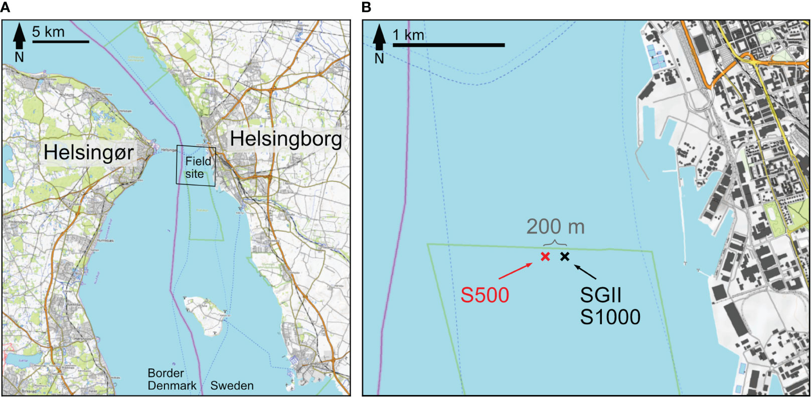
Figure 2 Overview of the field observation area in Oresund (A), located on the Swedish side of the strait. The black box indicates the location of the zoomed in map (B), where the location of the Signature 500 (S500), Signature 1000 (S1000) and Sea Guard II (SGII), are indicated. The approximate distance between the two instruments was ca 200 m. The shipping lane on the Swedish side is north bound.

2.1 Field observations in Oresund

The acoustic field observations were conducted between August 19–31 in 2020. Stratification observations were conducted between August 19–25. The experimental setup and configuration was the same as described in Nylund et al. (2021), with an upward-facing Nortek Signature 500 kHz (S500) broadband ADCP (ping frequency 1 Hz, cell size 1 m) placed on the seafloor, at 33 m depth, underneath the northbound shipping lane outside Helsingborg (lat N56.019233, lon E12.676900) (Figures 2, 3). In addition, a mooring with an Aanderaa SeaGuard II ADCP (SGII), close to the bottom at 32 m depth, and with a Nortek Signature 1000 kHz ADCP (S1000) (ping frequency 1 Hz, cell size 0.5 m), placed in a subsurface float about 22 m below surface, was deployed approximately 200 m east of the S500 instrument (lat N56.019283, lon E12.679683) (Figure 2B). The latter measured the water column between 2 and 20 m depth. Movements, changes in tilt and heading, of this instrument has to be post-compensated for. The SGII measured current velocities in the water column (ping frequency 0.25 Hz, cell size 0.5 m). In addition, this instrument was equipped with sensors to measure salinity/conductivity, temperature, pressure, waves, tide, and oxygen concentration close to the bottom. The 200 m distance between the instruments was chosen to cover a large part of the shipping lane, but still be close enough to observe the same ship passages in both instruments if the ship passed between the instruments. The distance was based on the observations by Nylund et al. (2021), where bubble wakes were frequently observed 3–6 ship widths from the passing ship, indicating that wakes from ships > 17 m wide should be possible to detect in both instruments when passing between them.Two small and fast leisure boats were used to access the instruments and passing ships. The water column stratification was measured using a handheld CTD SonTek CastAway®-CTD (Xylem, San Diego, California). During the study period, each day several profiles were measured at the location of the ADCP instruments at different times of the day. In addition, opportunistic stratification measurements in the wake of passing ships were conducted. First, 2–4 profiles were made before ship passage, and then 2–6 profiles were made in the ship wake as soon as possible after ship passage (usually 2–10 minutes).

Figure 3

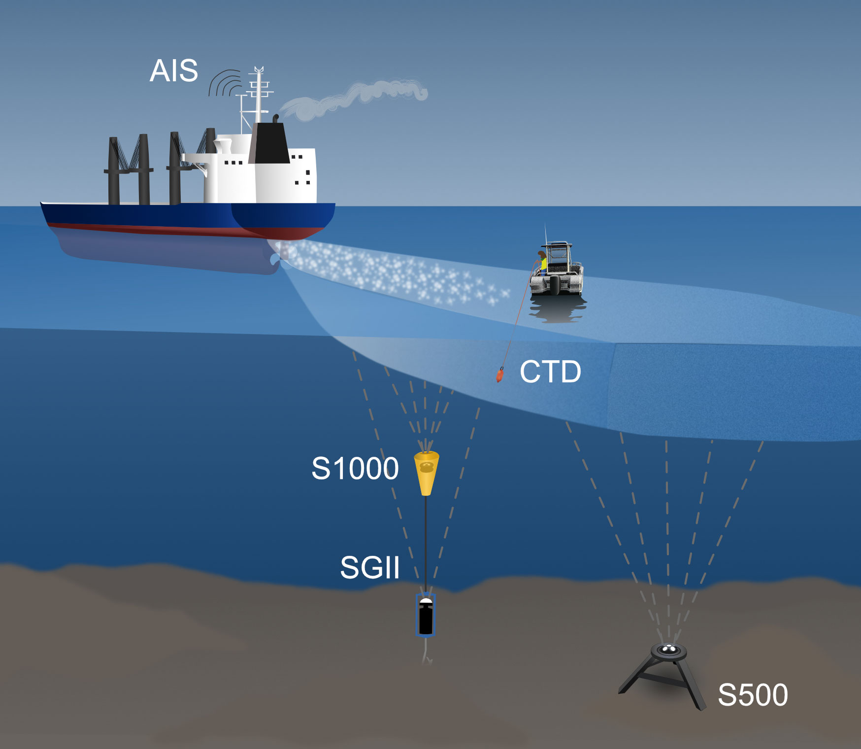
Figure 3 Illustration of the instruments used in the field observations. The Signature 500 ADCP (S500) was in a fixed stationary frame on the sea floor, whereas the Signature 1000 ADCP (S1000) and the SeaGuard II ADCP (SGII) were moored. Note that in the field, the instruments were placed on a line perpendicular to the shipping lane, and not in a line along the shipping lane. The illustration is not true to scale.

2.1.1 Additional datasets

To identify the vessels inducing the detected wakes, access to the Helsinki Commission (HELCOM) Automatic Identification System (AIS) database was purchased from the Swedish Maritime Administration (HELCOM, 2018). Detailed information about the vessels geometry and propulsion system was retrieved from the Sea-web Ships (2022) database. Observations from the study by Nylund et al. (2021) were included for comparison, and is available for download at https://doi.org/10.5281/zenodo.5066997 (Arneborg et al., 2021).

2.1.2 Analysis of field data

The wake detection and data analysis were conducted as described in Nylund et al. (2021). In short, the elevated echo amplitude from the bubbles in the turbulent wake region was used to identify the ship wakes in the ADCP datasets, and the AIS data was used to identify the ship inducing each detected wake. The dissipation rate of turbulent kinetic energy can be used as a measure of the intensity of the ship-induced turbulence, and of the mixing across density interfaces in a stably stratified water column. We estimated ε from the S500 and S1000 along beam current velocity observations, using the structure function method (e.g. Lucas et al. (2014)), as described in (Nylund et al., 2021). However, unlike (Nylund et al., 2021) the current velocities were not wave corrected. This was to retain as much of the ship-induced turbulence as possible and was assumed reasonable as the Oresund site was sheltered and the significant wave height during the observations was generally below < 1 m, half of the time < 0.5 m. As the top 2 m of the water column were excluded due to reflection from the water surface, we assumed that the majority of the detected energy in the remaining wake area originated from the ship and not from surface waves. The density observations from the CTD measurements were used to calculate the buoyancy frequency of the water column using the Thermodynamic Equation Of Seawater – 2010 (TEOS-10) software package Gibbs-SeaWater (gsw) Oceanographic Toolbox for Python (McDougall and Barker, 2011).

The echosounder and bow wave of the wake-inducing ships interfered with the current velocity observations of the ADCPs (see Figure 4 for example), and the initial 0.5–1 min of the turbulent wake were therefore excluded from the ε calculations. The structure function calculation required time averaging of the current velocities over 30 s, hence the resolution for the ε values was 30 s, compared to the echo amplitude and current velocity observations which had a 1 Hz resolution. The decay rate of ε was estimated by calculating the mean ε over 2–20 m depth, every 30 s for the first 10 minutes of the ADCP wake (i.e., start 0.5–1 min aft of the rudder). Only the top 20 m were included, as no wakes reached deeper than 20 m, and since the signal to noise ratio was higher in the deeper part of the water column, likely due to ambient noise from fish, plankton, and turbidity. The ε decay rate was estimated by a linear fit to the logged ε-values versus time.

Figure 4

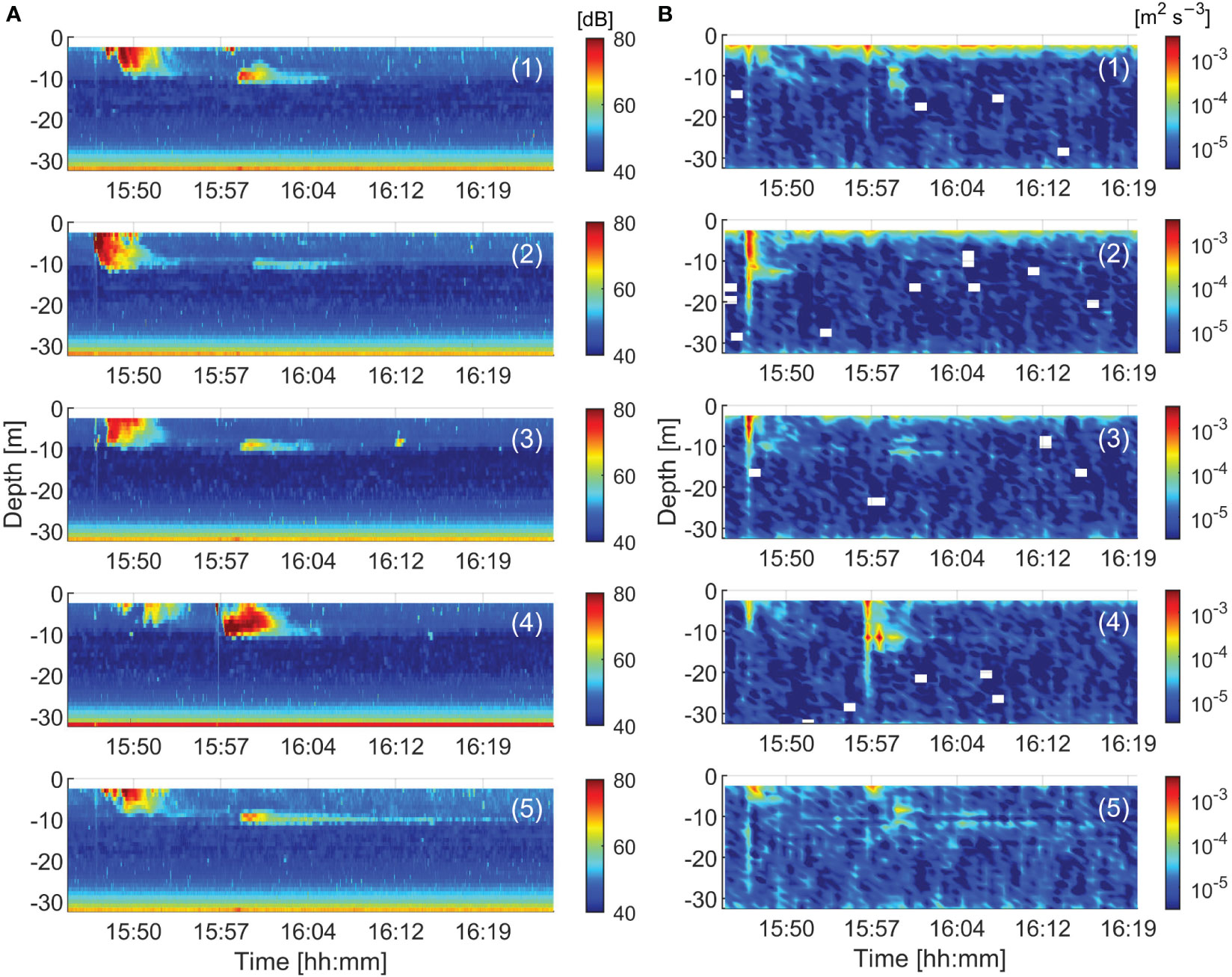
Figure 4 Example of an (A) echogram [dB] and (B) calculated ε [m² s^-3] for the five beams of the S500 ADCP (indicated by numbers 1–5), during the passage of a Ro-Ro Cargo (15:45) and Tanker (15:57) (for an illustration of the S500 beam configuration see Supplementary Figure 8). High yellow and red values indicate the wake areas. The thin vertical line visible at the start of the echogram wakes (A) is the echo sounder of the passing ship. A similar vertical line is visible in the ε figure (B), but in that case it is a combination of the echo sounder interference and the velocity changes induced by the ship’s bow wave (this section is excluded from the turbulence intensity analysis). In beam 3 (A) it is also possible to see the reflection of the ship hull as a small U-shape before the echo sounder line. The stratification depth was 10.5 m (Supplementary Figure 7B).

2.2 Ship wake modelling

To complement the field measurements, CFD simulations were performed of two different ships, in stratified and non-stratified conditions. The objectives were to get detailed information on the mixing incurred by the fluid motions caused by the propeller in the ship wake. Detailed ship data, such as hull design, draft, propulsion arrangement, or shaft rmp, were not available for any of the observed vessels.. Thus, two generic ship models were selected as representative vessels for ship types with different wake characteristics in the field observations, one single screw Tanker and one twin screw RoPax (ferry); ship data is listed in Table 1. These are two typical types of ships that navigate through the Oresund strait in which ships with a draft deeper than 8 m cannot pass.

Table 1

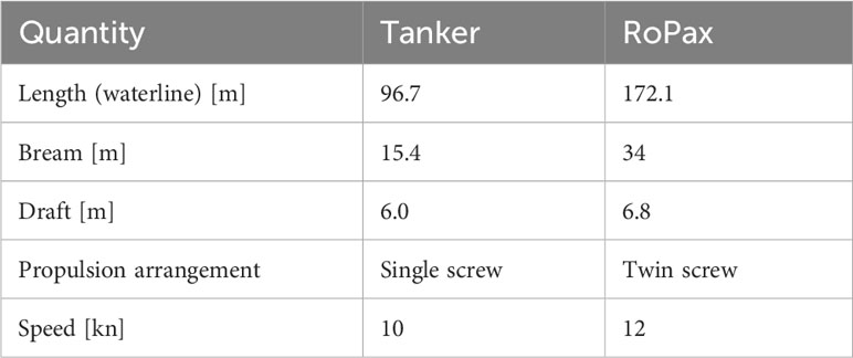
Table 1 Main particulars of the simulated ships.

The ships were simulated in full-scale using RANS modelling and the k-ω-SST turbulence model with wall functions (Menter et al., 2003). The open source libraries of OpenFOAM were used to perform the simulations (Weller et al., 1998). Stratification was modelled using a Boussinesq approximation, deemed valid for the density variations that are considered. Temperature profiles and thermal expansion coefficients, primary solver quantities, were developed to represent the stratification from the field observations for the days August 19 and August 21 2020, giving three different conditions for the simulations: one without stratification, one with shallow and smooth density variation, and one with deeper but sharper variation (Supplementary Figure 2).

In order to capture the rotational effects of the propeller on the ship wake, resolved rotating propellers were used in combination with a refinement box stretching aft of the ship for several ship lengths. However, to save computational effort, the ship generated waves were not resolved. For the objectives in this study the ship waves are not expected to be important, and the computational overhead would be extensive. Mesh sizes were 33 M cells for the Tanker and 30 M cells for the RoPax; for the RoPax, being a twin-screw vessel, only half the hull was simulated with a symmetry plane. Simulations were run for more than 30 s real time with a time step corresponding to less than 1° of propeller revolution.

2.3 Total ship-induced turbulent kinetic energy dissipation rate

An estimate is the total ship-induced power [kW] in the turbulent wake was calculated using the field observations of ε in the far wake and the model output of the near wake, for a Tanker and RoPax vessel. From the field data, a Tanker and RoPax passage from August 19 were chosen, as the ship dimensions and stratification were similar to the model cases (Supplementary Figure 2). The observed tanker was 95 m long, 13 m wide, having a 6 m draught, and installed engine power of 2 380 kW, and the RoPax 178 m long, 30 m wide, with a draught of 6 m, and an installed engine power of 23 760 kW. The total power ($P_{tot}$) for the far wake of the two ships was calculated for each beam ADCP beam according to Equation 1:

$\begin{array}{ll}{\mathit{\text{P}}}_{\mathit{\text{tot}}}={\sum }_{\mathbf{0}\mathit{\text{s}}}^{\mathbf{600}\mathit{\text{s}}}({\sum }_{\mathbf{20}\mathit{\text{m}}}^{\mathbf{2}\mathit{\text{m}}}({\epsilon }_{\mathit{\text{avg}}}·{\mathit{\text{u}}}_{\mathit{\text{s}}}·{\rho }_{\mathit{\text{sw}}}·\mathit{\text{w}})·\mathit{\text{Δd}})·\mathit{\text{Δt}}& (1)\end{array}$

where ${\epsilon }_{avg}$ is the observed $\epsilon$ values in each 1 m ADCP bin ($\Delta d$) for the initial 10 minutes of the wake, $\Delta t$ is the time step between the $\epsilon$ values (30 s), $u_s$ is the ship speed in m s^-1, ${\rho }_{sw}$ is the seawater density observed in the surface mixed layer (1010 kg m^-3), and $w$ is the wake width in m (estimated to twice the ship width). The values were summed over 2–20 m depth and 600 s to estimate the total observed effect in the entire far wake region. The power in the near wake was calculated using Equation 1, with the $\epsilon$ output from the simulations the centreline just behind the propeller as ${\epsilon }_{avg}$, $w$ equalling 1 m, a$\text{Δ}t$ of 7.2 s, and the modelled ship speeds (Table 1). The total power in the wake was then calculated as the sum of the near and far wake estimates and related to the ship’s installed engine power.

3 Results

3.1 Field observations in Oresund

Background measurements of currents (0–160 cm s^-1, main transport towards south southeast (SSE)) (Figure 5), waves (0–1.4 m significant wave height), tides (10–20 cm), bottom salinity (~33 PSU), bottom temperature (~10°C) and bottom water dissolved oxygen (~33% air saturation) was carried out by the SGII-ADCP instrument that was logging every 10 min for the entire period (Supplementary Figure 3). Most of the time, the ships in the shipping lane had a counter current (SSE), but occasionally it was in the same direction as the ship’s heading (north northwest, NNW) (Figure 5B). During the initial part of the study period (19–22 August), the weather was calm with significant wave heights close to 0 m, but the latter part (August 23–26) had strong winds and significant wave heights of 0.5–1.4 m, which caused increased noise in the ADCP measurements (Supplementary Figure 3).

Figure 5

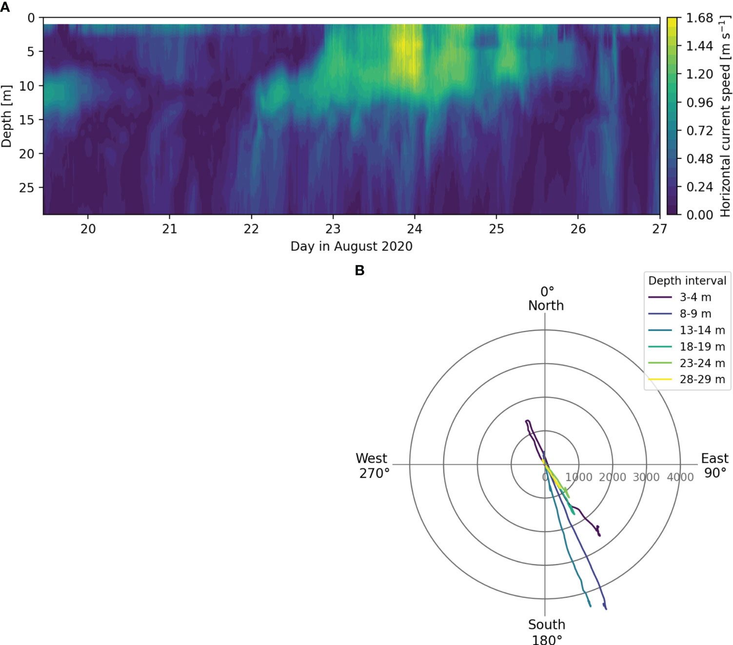
Figure 5 (A) Horizontal current speeds [m s^-1] in Oresund (SeaGuard II ADCP) during the period included in the wake analysis (Aug 19–26, 2020). Speeds were measured at every meter from surface to 30 m depth. The top observation (0–1 m) is excluded due to interference from the sea surface. (B) Progressive current vectors in Oresund at six different depths below surface (indicated by color legend), observed with the SeaGuard II during the sampling period Aug 19–31, 2020. Note that the current direction is alternating between south southeast (150°) and north northwest (330°).

The CTD observations showed salinities ranging from 9–16 PSU above the stratification and 32.5–33.5 PSU below, resulting in strong density gradients (Supplementary Figures 4, 5). The water temperature ranged from 19–22°C above the stratification and 10–13°C below, thus a clear temperature gradient of ~9–11°C over 2–10 m (Supplementary Figure 4). The pycnocline was located between 7–20 m depth, and the thickness varied from a few meters up to 10–15 m (Supplementary Figure 5). A total of 13 CTD measurements of the stratification inside and outside the turbulent wake were also made. However, none of the CTD observations showed any conclusive indications of ship-induced mixing. This was partly due to the large natural variability in the stratification depth, which oscillated slowly up and down. The other factor was the strong stratification, which made the adjustment period and re-stratification after ship passage very short and near impossible to sample. When the ADCP instruments were retrieved, the distance between them were closer to 300 m than 200 m, indicating that the instruments had a slightly different location than indicated in Figure 2. Therefore, a visible reflection of the echosounder or hull of the passing ships, was used to identify the ships passing right over the instrument. The increased distance meant that the two instruments were too far from each other to observe the same wake, although simultaneous ship-induced internal waves were sometimes observed. Consequently, it was not possible to estimate the maximum wake width by combining the observations from the two instruments. However, the median width of the sampled ships (17 m) indicate that the intended distance of 200 m would have been suitable.

In the S500 and S1000 ADCP measurements, 55 clear wakes were detected (S500: 30, S1000: 25), as well as 19 passages with clear internal waves. Ship passages were also detected by the SGII wave and tide pressure sensor, as a ship-induced drop in pressure of ca 15–20 mbar (see Supplementary Figure 6 for example). However, as the sensor only measured during 64 s every 10 min, only a few passages occurred during the sampling window. The ε wakes were slightly deeper than the bubble wakes, ~10 m compared to ~12 m, and the media and variation were similar for both instruments (Figure 6). The S500 median bubble wake duration (9 min and 45 s) was longer compared to the S1000 bubble wakes (6 min 23 s), and the ε wakes (ca 4 min) (Figure 6).

Figure 6

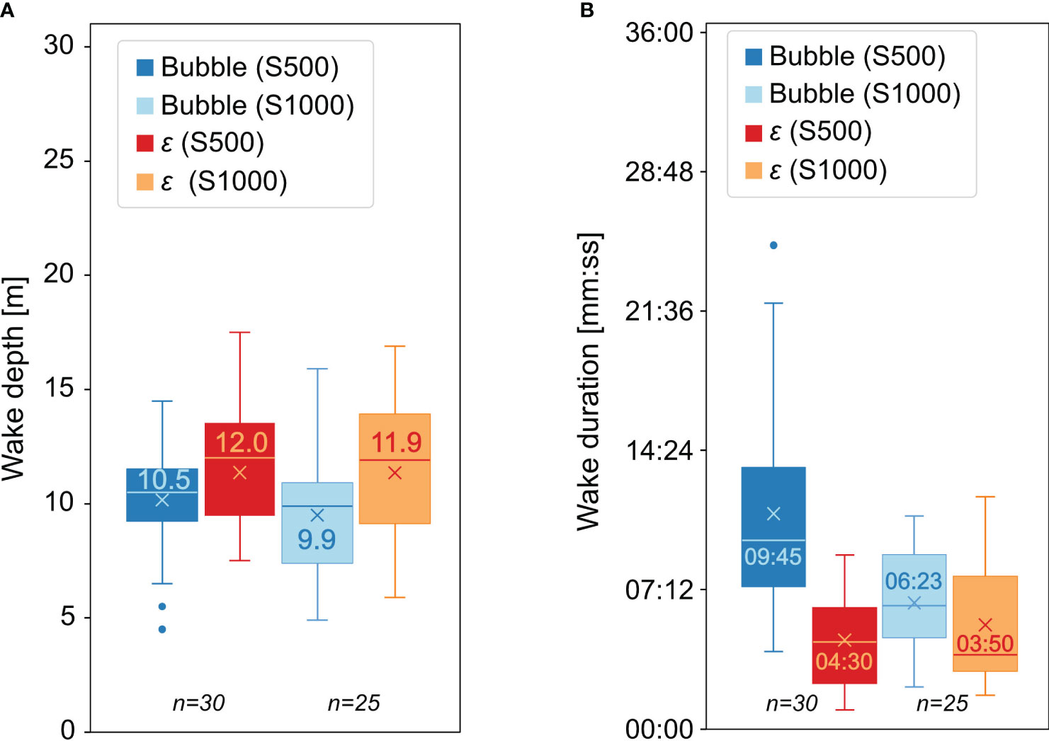
Figure 6 Bubble and ε wake depths [m] (A) and duration [mm:ss] (B) for the S500 and S1000 observations. The sample size (n) was 30 wakes for S500 and 25 for S1000. The vertical line and number indicate the median value, and the x marks the mean value.

3.1.1 ADCP observations of the interaction between stratification and the turbulent wake

The ADCP observations showed that the ε wake frequently penetrated a few meters below the stratification. In the S500 data there were 6 clear examples of turbulence reaching below the observed stratification, corresponding to 25% of the detected passages with visible echosounders (see Figure 7 for example). In the S1000 data, there were 5 clear examples of turbulence penetrating the stratification, corresponding to 36% of the analysed passages.

Figure 7

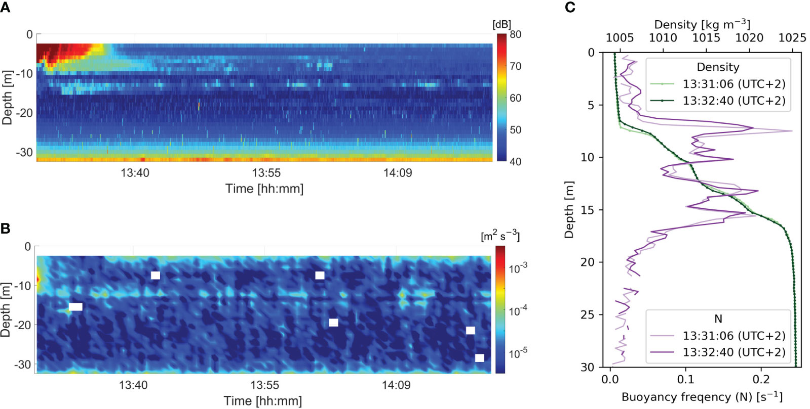
Figure 7 Example of bubbles (A) and turbulence (B) reaching below the stratification located at 8 m depth (C). In (A) and (B) the x-axis shows the time [hh:mm] and the y-axis the water depth [m]. The top 2 m are excluded due to interference from surface reflection. The ship inducing the wake was a RoPax vessel (speed 17 knots, draught 6 m, length 178 m, width 30 m). The y-axis in (C) shows depth and the x-axis shows the density [kg m^-3] (green dotted lines) on the top and Buoyancy frequency [s^-1] (purple lines) on bottom. The density profile was observed just before the ship passage and the Buoyancy frequency was calculated based on the density profile.

The stratification was also affected through the generation of ship-induced internal waves, which were observed 29 times (both instruments) (Figure 8). The internal waves were induced by close ship passages, with visible bubble/ε, wakes at the instrument site, and by ships at 100–350 m distance from the instrument, lacking visible bubble/ε wakes. Hence the internal waves affected the pycnocline in a large area by moving the pycnocline vertically. There was a 2–3 min delay after the ship passage before the internal wave reach the instrument at ~15:22 p.m., which indicates an internal wave horizontal group speed of approximately 1.1–1.7 m s^-1. There were no observations of mixing caused by the internal waves, but it is well known that internal waves do contribute to mixing when they decay due to instabilities or interactions with bathymetry or the background flow field. The energy flux and conditions when these internal waves appear will be studied in a separate paper.

Figure 8

Figure 8 Example of a ship-induced internal wave observed with the S500 instrument 25 August 2020. The x-axis shows the time [hh:mm] and the y-axis the water depth [m]. The 2 m closest to the water surface are excluded due to interference from surface reflection. The internal wave was induced by a large cruise vessel (draught 9 m, width 45 m, length 334 m, speed 13 knots) passing at 15:19 p.m. at a distance of 200 m. The stratification depth was approximately 9 m (Supplementary Figure 7A).

There were clear indications that the bubble and turbulent wake development was impacted by the stratification and/or currents. Figure 4 is an example of a type of interaction between the turbulent wake and stratification, which was observed multiple times (for an illustration of the S500 beam configuration see Supplementary Figure 8). The second wake in the figure, induced by a tanker (start 15:57 p.m.), is an example of when vertical mixing has brought up denser water from below the stratification and created a new, denser water mass, which distributes horizontally along the pycnocline (here at 10.5 m). The horizontal spread is visible as an elevation at 10 m depth in beam 1, 3, and 5 in the ε wake (B), and it is clear in all beams of the bubble wake (A).

There were also clear indications that the hydrography (stratification and currents) restricted the vertical extent of the wake development, as a majority of the wakes had a relatively sharp and flat bottom which closely followed the stratification (see Figures 9, 10 for examples). Figure 9 shows the variation in bubble wake development for three similarly sized Ro-Ro Cargo vessels with similar speeds, during different stratification and current. The top figure is from the Oresund S500 observations and the middle and bottom figures are from the observations by Nylund et al. (2021) in 2018, where the same S500 instrument was placed at a similar depth in a shipping lane outside the port of Gothenburg.

Figure 9

Figure 9 S500 bubble wake development for three Ro-Ro Cargo ships of similar size, for different hydrographic conditions. The x-axis indicates time [hh:mm] and the y-axis shows water depth [m]. The top 2 m are excluded due to interference from surface reflection. (A) Oresund, stratification depth 8 m (Figure 7C). Note the comparatively flat bottom edge of the wake at the same depth as the stratification. (B) Gothenburg, stratification depth 5 m (Supplementary Figure 7C), and (C) Gothenburg, unknown stratification. Note the intermittent and varying bottom edges of the two Gothenburg wakes. For vessel details and ε wake see Supplementary Figure 9.

Figure 10

Figure 10 S500 bubble wake development for two similarly sized General Cargo vessels. (A) Oresund, stratification at 8 m depth (Supplementary Figure 7A) and (B) Gothenburg, stratification at 5 m depth (Supplementary Figure 7C). For vessel details and ε wakes see Supplementary Figure 10.

In the Oresund observation (A), there was a strong stratification at 8 m depth (Figure 7C), below which there was a strong south going current of about 0.4–1 m s^-1 (Figure 5A). The Oresund wake appears limited and compressed vertically, compared to the Gothenburg wakes, indicating that the difference in hydrographic conditions have an impact on the vertical extent of the wake. In the middle Gothenburg case (B), the current velocities were low (< 0.2 m s^-1) and there was a clear, but weaker stratification at 5 m depth (Supplementary Figure 7C). The ship draught of 7 m exceeded the stratification depth, which could potentially explain the deep penetration of the wake. For the bottom Gothenburg case (C), there was no available stratification observation, but it illustrates the large variation in turbulent wake development for comparable vessels, indicating the impact of hydrography on wake development. This difference was also noticable in the ε wake development, although not as clearly (Supplementary Figure 9).

A comparison was also made for the wake development of two similarly sized General Cargo vessels with similar speeds (Figure 10). In the top panel (A) there was a stratification and southernly current (0.5–0.7 m s^-1) at 8 m depth (Supplementary Figure 7A and Figure 5A), and a slightly shallower wake extent compared to the bottom panel. In the bottom panel (B) the current velocities were very low (< 0.1 m s^-1), and there was a weak stratification at 5 m depth (Supplementary Figure 7C), which the ship draught exceeded. In this example the Oresund ε wake was not very large, but there is an indication of the same tendency as for the bubble wake (Supplementary Figure 10).

3.1.2 Turbulent wake development

Of the 55 turbulent wakes (Figure 6), only the wakes with visible ship echosounder reflections in at least three beams were included in the ε decay analysis, as they were assumed to be induced by ships passing right over the instrument and represent the core part of the wake. As the slanted beams in the S1000 data were very noisy compared to the S500, probably due to the movement caused by the mooring setup, only the S500 dataset was used in this analysis, resulting in a total of 22 wakes.

The observed and modelled ε decay rate, for the 9 wakes in the S500 dataset with a visible ship echosounder signal in all five beams, is presented in Figure 11. The plotted values (open circles, ADCP data) are the mean ε over 2–20 m depth, at each time step. Due to echosounder and bow wave interference, the calculated ε values were only available from 0.5–1 min aft of the rudder, therefore a 30 s delay was added to the plotted data to illustrate the time relationship between the model result and field observations. The linear fit to the logged data (black dashed line) had an R²-value of 0.46 and was in very good agreement with the dataset mean (red line). The linear fit corresponds to an exponential decay rate (-0.64) which is quite similar to that obtained by Milgram et al. (1993) (-0.8). Included for comparison are the modelled ε values for first 30 s of the wake (see section 3.2). The 9 wakes in the figure were induced by five different ship types (Ro-Ro Cargo, RoPax, Tanker, General Cargo, Vehicles Carrier) with similar draughts, but of varying size and speed. Despite this, the ε decay rate was very similar for all passages, indicating that ship type, size, and speed did not significantly affect the observed ε values. To investigate potential ship-type differences, the ε decay rate for the ship types with more than 3 wakes were also analysed (Supplementary Figure 11). Similar to Figure 11, there were no clear differences between the ship types.

Figure 11

Figure 11 The mean decay of turbulent kinetic energy dissipation rate (ε), for all ships with a visible echosounder in all 5 beams (S500). The ε mean was calculated over 2–20 m depth for each ADCP beam, and then the mean of all beams was calculated (circles). The red line is the datapoint mean, and the red area indicates the 95% confidence interval (CI) of the mean. A linear function f(x) is fitted to the logged data (black line). The model output of mean ε from the rudder position (10⁰) and 30 s onwards for the Tanker (dark blue dashed dotted line) and RoPax (light blue line), both for the 200819 stratified case. As the field observations start 0.5–1 min aft of the rudder, a 30 s delay have been added to the field observations to illustrate the time relationship between the model result and field observations.

Exposure of ε levels above 2.5$·$10^-4 m² s^-3 for more than 45 s has been found to increase plankton mortality (Bickel et al., 2011; Garrison and Tang, 2014). This ε threshold value was exceeded in 55% of S500 wakes, and 50% of the S1000 wakes (data not shown). Few of the S500 passages had ε values exceeding 1$·$10^-3 m² s^-3, and the duration of the occurrences of ε values above the threshold level were mostly very short (30 s–1 min). In the S1000 data, all but one of the passages exceeding the threshold had ε values > 1$·$10^-3 m² s^-3, and the duration of the high ε values were longer (2–10 min) compared to the S500 wakes. The threshold levels were exceeded at the surface of the wake, over the entire wake depth, or only along the stratification without a surface signal (as exemplified in Figure 4). The ship-induced ε values at the pycnocline reached deeper and were higher than the observed wind generated turbulence during the windy sampling period (see example in Supplementary Figure 12). Overall, the S1000 data recorded higher ε values compared to the S500 instrument.

3.2 Ship wake modelling

3.2.1 Modelled turbulent wake development and intensity

The model output of ε decay rate in stratified conditions (19 August 2020 case, Supplementary Figure 2) is included in Figure 11, for comparison with the field observation. The model output was averaged over the same depth interval as the ADCP data, for the wake centreline (Tanker) and aft of one of the propellers (RoPax). The first 30 s of the wake had the highest ε values, and they were two orders of magnitude larger than the observed values. In the temporal range where the model and observed values meet, there was a good agreement between the Tanker output and observed values, whereas the RoPax model output had higher ε values compared to the observed data (Supplementary Figure 11).

The modelled ε decay rate for the Tanker in homogenous and stratified water showed a more variable and slightly faster decay rate for the stratified cases (August 19 and 21 2020, denoted 200819 and 200821 respectively), although the 200821 case converged with the homogenous case after ca 15 s (Figure 12). For the RoPax, the homogenous case had a higher maximum value, but after 10 s the decay rate was similar for the two cases (Figure 12). Comparing the Tanker and the RoPax ε decay rate, the RoPax had a much higher maximum ε value, but the decay rate was similar for both ship types (Figure 12). In both the stratified and non-stratified case, the decay rates were similar to (-7/3), as previously reported by Wall and Paterson (2020) and Brucker and Sarkar (2010).

Figure 12

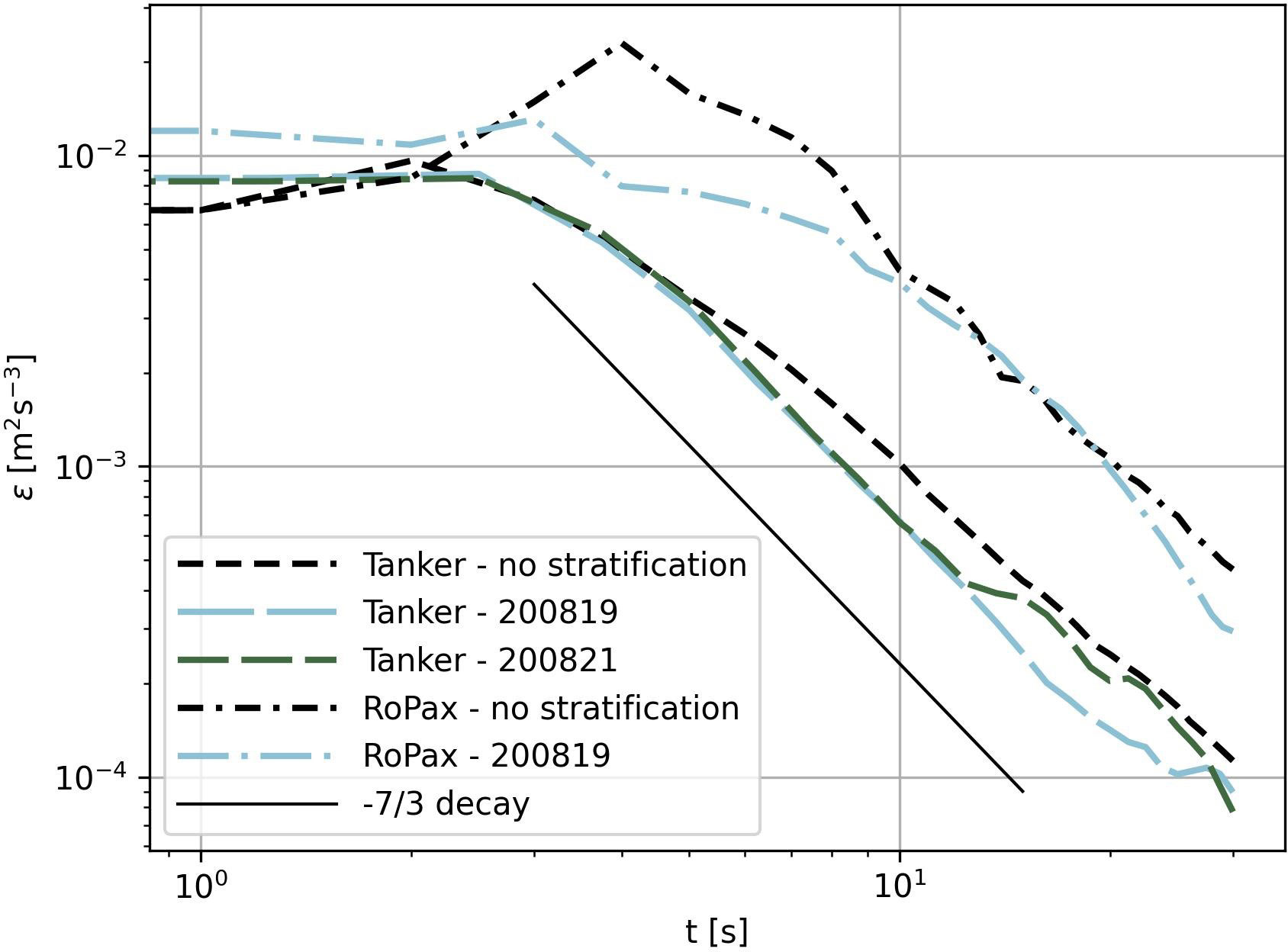
Figure 12 Modelled mean ε values over 2–20 m depth for a 1 dm² area, for the first 30 s of the wake from the rudder position (10⁰) and 30 s onwards. The mean was calculated for the wake centreline (Tanker) and aft of one of the propellers (RoPax). Black lines are the mean ε values without stratification for the Tanker (dashed line) and RoPax (dashed dotted line). Light blue lines are the 200819 stratified scenarios for both ship types, and the green dashed line is the 200821 stratified scenario for the Tanker. The (-7/3) ε decay rate is included for comparison (thin black line).

For both ships, the maximum ε values declined substantially at either side of the propeller centre line (Supplementary Figures 13-15). The peak in ε at the sides showed a clear delay compared to the centre line, indicating a speed of the sidewards expansion of the turbulent wake of 10 m and 7 m in 30 s for the RoPax and Tanker respectively. For the Tanker, the ε peak was higher at the port side compared to the starboard side (Supplementary Figures 13–15). This likely relates to the interaction between the propeller rotational direction (clockwise) and rudder, which caused the propeller slip stream to split, and where the port side vortex was directed downwards and the starboard side upwards (Supplementary Figures 16, 17, homogenous case). The RoPax also had higher values on the port side of the propeller, but the difference was smaller, and 5 m port side of the RoPax propeller corresponds to 2 m from the centre line, thus not directly comparable with the Tanker case (Supplementary Figure 13, Figure 13).

Figure 13

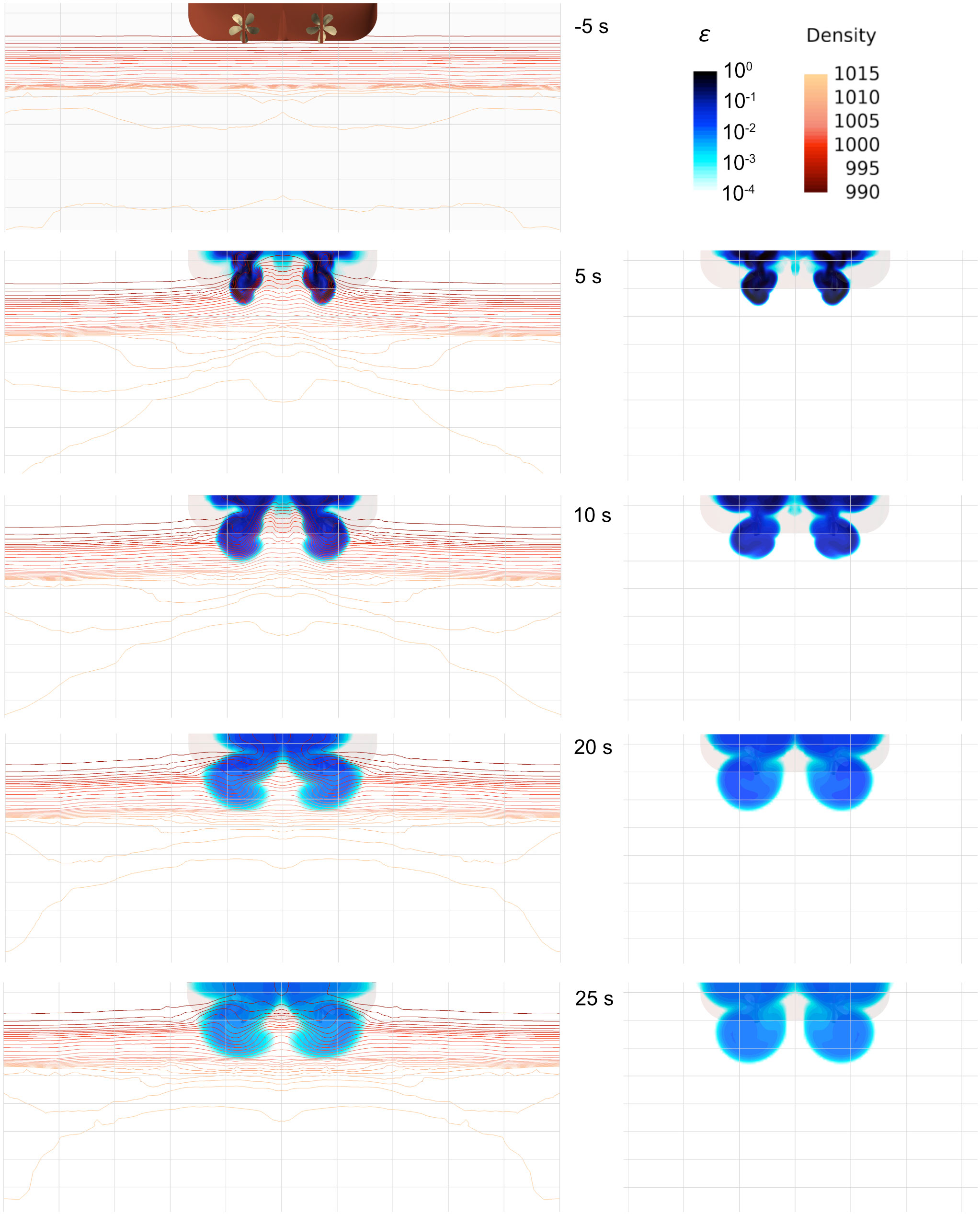
Figure 13 Cross-section of the ε wake 5, 10, 20, and 25 s aft of the RoPax for the 200819 stratification case (left) and homogenous case (right). Red lines indicate density [kg m^-3] and blue color the ε intensity [m² s^-3]. Distance between horizontal and vertical grid lines is 5 m.

3.2.2 Interaction between stratification and the turbulent wake

The Tanker and RoPax model output clearly show that the stratification is influenced by the ship passage (Figure 13; Supplementary Figures 14, 15). The main vertical movements are caused by displacement of water due to the ship and it is difficult to directly see mixing from isopycnal displacements (Supplementary Figures 16–18). However, the large dissipation rates in the strongly stratified fluid are clear indications of strong/intense mixing. The higher density in the surface layer directly after the ship passage (Figure 14) is also indicative of entrainment into the surface layer. The effect was clearest for the RoPax case. There were no evident signs of the stratification vertically restricting the ε wake development, on the contrary, the Tanker 200821 case had a slightly deeper wake compared to the non-stratified Tanker case (Supplementary Figures 19, 20).

Figure 14

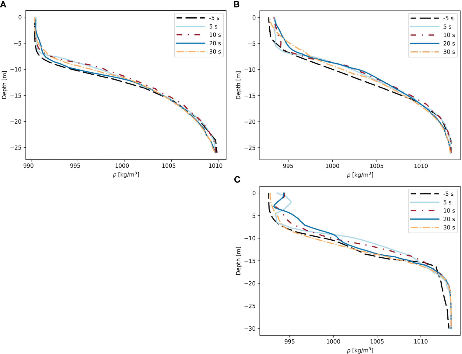
Figure 14 Density profiles (ρ) [kg m^-3] for the propeller centerline from before ship passage (-5 s, black dashed line), and at four times after passage: 5 s (light blue), 20 s (red dashed dotted), 20 s (dark blue), and 30 s (orange dashed dotted). (A) is the 200821 Tanker case, (B) is the 200819 Tanker case, and (C) is the 200819 RoPax case. There is a clear change in the density profile above the stratification (approximately 6 m for 200819 and 10 m for 200821, Supplementary Figure 2) in both (B) and (C), with the RoPax having the largest impact.

3.3 Total ship-induced turbulent kinetic energy dissipation rate

For the far wake, the mean calculated power and standard deviation for the ADCP beams was 32 $\pm$7 kW for the Tanker and 146 $\pm$25 kW for the RoPax. The near wake power calculations based on the model output, gave a power of 3002 kW for the RoPax (two times 1501 kW) and 418 kW for the Tanker, resulting in a total power for each wake of 3148 $\pm$25 kW for the RoPax and 450 $\pm$7 kW for the Tanker. This corresponds to 13% and 19% of the installed engine power for the RoPax and Tanker, respectively.

4 Discussion

4.1 Interactions between stratification and the turbulent wake

The field observations clearly showed that stratification affected the turbulent wake development and caused the wake to spread horizontally along the stratification, instead of expanding vertically (Figure 4). This horizontal spread can be explained by two different processes, where the first one (exemplified in Figure 4) is the entrainment of deeper water from below the pycnocline. The vertical mixing across the pycnocline entrains denser water into the wake region, and the wake water becomes denser compared to the surrounding surface water. The increased density of the wake water, leads to a downward movement of the wake water (and bubbles entrained in the wake) towards its new equilibration depth. Due to the strong stratification, this new equilibration depth will be close to the pycnocline, resulting in the wake water layering/spreading horizontally along the stratification. This process was observed on several occasion in both the S500 and S1000 instrument and is evidence of ship-induced vertical mixing across the pycnocline. This was supported by our model results, which showed that both the Tanker and RoPax caused entrainment, with the largest effect/impact in the RoPax case (Figure 14). To our knowledge, this process has never previously been observed in the field. However, Jacobs (2020) modelled propeller wakes in a stratified fluid, and also found that the propeller would create mixing across the stratification, as well as entrain water from the side of the wake. Moreover, Merritt (1972) observed the same entrainment effect in model scale experiments, where a dye was released in turbulent wakes in stratified and non-stratified fluid to observe the wake development. They also found a decreased vertical spread and increased horizontal spread and, furthermore, noted that the dye in the thin stratified wake appeared to dilute slower compared to the unstratified case.

The second process affecting the turbulent wake development, is the impeding effect of a stratification and/or strong currents. When comparing the Oresund observations with previous observations by Nylund et al. (2021) outside Gothenburg, the vertical extent of the Oresund wakes were restricted and “flattened” in comparison (Figures 9, 10). As the ship-specific parameters size, type, and speed, were similar for the compared cases, the difference in vertical extent was likely due the difference in hydrographic conditions. Although both sites had a stratification, the Oresund stratification was much stronger (see Supplementary Figure 7), which is a likely explanation for the difference in vertical wake extent between the sites. The stratification outside Gothenburg in Nylund et al. (2021) was also shallower than the ship draughts, hence, the ship hulls observed outside Gothenburg would extend below the pycnocline. This could potentially also contribute to the deeper wakes and more intermittent and irregular wake shape, compared to the Oresund wakes, but the difference in stratification is likely the main cause. It is well known that strong stratification impede the vertical and expand the horizontal extent of the wake (Merritt, 1972; Lin and Pao, 1979; Brucker and Sarkar, 2010; Jacobs, 2020), hence our dataset could provide the first observations of this process in the field for full-scale ships.

However, the large difference in current speed could also be a potential explanation to the difference in wake development between the sites. The strong, southernly counter current at the stratification depth in the Oresund cases, could potentially drag the wake towards the aft, and thereby limit the vertical extent and favour a more horizontal expansion. Loehr et al. (2001) observed asymmetric bubble wakes, which they hypothesised were caused by the strong current shear at the site, as the wakes were spreading in the direction of the current. Similar to the observations in Figure 4, the wake in Loehr et al. (2001) was observed to only expand horizontally at depth, and not uniformly in the entire water mass, creating an asymmetric L-shaped wake development. However, in the Loehr et al. (2001) wake, this elongation was only observed at one side of the wake (in the current direction), unlike our observations in Figure 4 which showed elongation at depth on both sides, indicating a radial or upside down T-shaped wake development perpendicular to the current. This difference implies that the current shear is a likely explanation to the asymmetric wake development observed by Loehr et al. (2001), and that currents can affect the wake development. Weber et al. (2005) is the only other previous study where the stratification depth was similar to the wake depth, but the surface current velocities were very low, and they reported no observations of vertical limitations of the wake development. Based on the Oresund field observations, it is not possible to determine if the entrainment or current affected the wake development most, especially since the stratification and high velocity current were located at the same depth. Nevertheless, it is likely that both of these processes impact the spread of the turbulent wake and the wake water. Unlike the field observations, our model results did not show a clear vertical restriction or horizontal spread of the wake (Figure 13; Supplementary Figures 14–20). However, the field observations showed that the deepest part of the turbulent and bubble wake often occurred more than 30 s after ship passage, as it takes time for the wake to move downward (see examples in Supplementary Figure 9 and Figure 4). This could explain the discrepancy between the field observations and the modelling results and highlights how CFD modelling of the near wake only, is not sufficient for estimating the maximum vertical extent of the turbulent wake.

The observed internal waves were expected, as ships in stratified water are known to induce internal waves (Lin and Pao, 1979; Watson et al., 1992; Jacobs, 2020), and the estimated internal wave speed of 1.1–1.7 m s^-1 is realistic for these strongly stratified conditions. A rough estimate of the long internal wave speed is (g’h)^1/2 where h is the surface layer depth and g’ = g (ρ₂ - ρ₁)/ρ₂, with g the gravitational acceleration, and ρ₁ and ρ₂ the surface and bottom layer densities. With a difference between surface and bottom layer densities of about 15 kg m^-3 and a surface layer depth of 10 m, one obtains a wave speed of 1.2 m s^-1. Watson et al. (1992) used ships of three different sizes to induce and study internal waves in a stratified sea loch and found that the largest ship (180 m long) induced the largest internal waves and a stronger stratification led to larger wave amplitude. Two of the largest and clearest internal waves, detected in both S500 and S1000, were induced by the two largest vessels in the dataset; two 334 m long cruise ships (see one of them in Figure 8). Yet, detectible internal waves were induced by ships of all sizes, although mostly by ships > 100 m long, and not all large ships induced internal waves. The stratification was strongest the 21^st and 23^rd, and many of the internal waves were detected the 23^rd, but a large part of the internal waves was detected the 25^th, including the largest ones. Hence our results were in line with, but not fully in agreement with the observations by Watson et al. (1992).

4.2 Turbulent wake extent and development

The median wake depths were similar for the S500 and S1000 observations, with an ε median depth of 12 m and a bubble median depth of ~10 m (Figure 6). The wake depths were in line with observations by Nylund et al. (2021), who reported ε and bubble wake depths at 13.5 m and 11.5 m respectively. The slightly larger depths of the ε wakes, could have several causes. Firstly, the buoyancy of the larger bubbles could counteract the downward vertical mixing (Trevorrow et al., 1994; Weber et al., 2005), and potentially decrease the maximum depth the bubble will reach. However, the smaller bubbles of the wake would still be fully trapped by the wake turbulence for several minutes (Stanic et al., 2009), and would be expected to extend to similar depths as the turbulence. The depth difference could also be an artefact of the relatively coarse depth resolution of the observations (1 m bins for S500 and 0.5 m bins for S1000) and the ε calculation, as the ε estimate is influenced by neighbouring cells. Strong turbulence in one cell could result in calculated levels of turbulence in a calm, neighbouring cell. However, as S1000 with the highest depth resolution had a larger difference in wake depth median value between the ε and bubble wake (Figure 6), it could be an indication that the calculation method is more likely to underestimate than overestimate the ε wake depth. Nevertheless, due to the limited ADCP bin resolution, waked depth differences smaller than 1–2 m should not be considered significant.

A handful of studies have observed the bubble wake depth (NDRC, 1946; Trevorrow et al., 1994; Loehr et al., 2001; Weber et al., 2005; Stanic et al., 2009; Ermakov and Kapustin, 2010; Soloviev et al., 2010; Soloviev et al., 2012; Francisco et al., 2017). A majority of these studies reported bubble wake depths of 3–12 m, and two studies observed wake depths down to 18 m (Loehr et al., 2001; Soloviev et al., 2010). Our observed bubble wake depths were thus in the same range as previously reported, but at the deeper end of the scale. Comparing the turbulent wake extent with the observed wind/wave induced turbulence during the measurement period, the wind-induced bubbles and turbulence seldom reached below 5 m, and never as far as the stratification (Supplementary Figure 12).

The wake duration differed between the ε and bubble wake and between the two instruments (Figure 6). The difference in bubble wake duration between the S500 (9 min 45 s) and S1000, was likely due to the frequency difference between the two instruments. Small bubbles have a higher resonance frequency than large bubbles (Liefvendahl and Wikström, 2016), hence the smaller bubbles captured by the S1000 (1000 kHz) would dissipate faster compared to the slightly larger bubbles observed by the S500 (500 kHz) (Trevorrow et al., 1994). For S500, the median bubble wake duration of 9 min 45 s was clearly longer than for the ε wake with 4 min 30 s, indicating that the longevity of the bubbles exceeds that of the turbulence/ε. Similar wake durations and a longer bubble wake than ε wake, were also found by Nylund et al. (2021), and the bubble wake durations were within the range of previous studies (NDRC, 1946; Trevorrow et al., 1994; Loehr et al., 2001; Weber et al., 2005; Stanic et al., 2009; Ermakov and Kapustin, 2010; Soloviev et al., 2010).

4.3 Turbulent wake intensity and decay

The highest mean ε values in the ADCP observations were ∼10^-4 m² s^-3 (Figure 11), which were calculated for 2–20 m depth. As < 25% of the observed wakes had depths > 15 m (Figure 6), the maximum ε values would likely be larger, as part of the water depth included in the analysis would be outside the wake influence. After ca 300 s from the first ADCP observation, the ε values had usually decreased to the instrument noise levels again. The turbulent intensity in the first 30 s of the wake was estimated using CFD modelling and showed maximum mean ε values of $\sim$10^-2 m² s^-3 for both ship geometries, but the RoPax had higher values (Figure 12). The modelled maximum ε values were more than two orders of magnitude larger than the maximum values calculated from the ADCP observations, indicating that the initial 30 s of the wake were the most turbulent, as could be expected for propeller generated turbulence. At the end of the initial 30 s, where the observed and model values converge, there was a very good agreement between the observed values and the Tanker case, but the RoPax values were ~5 times higher (Figure 11 and Supplementary Figure 11). The difference in ε magnitude between the two ship types in the model output was expected, as the ships had different size and propeller configuration (Table 1). The RoPax geometry was twice the length and width of the Tanker and would thus be expected to induce more turbulence. The RoPax also induced much larger vertical velocities (Supplementary Figures 16–18), although a large part of that movement was due to water displacement rather than mixing. In addition, the RoPax had two propellers, thus inducing intense turbulence over a larger area than a single propeller (Figure 13; Supplementary Figures 14, 15). Still, as the twin-screw configuration would mainly affect the total ε of the wake and not the mean ε values plotted in Figures 11, 12, it is likely not the main cause of the higher ε values for the RoPax in the model output. In contrast, the field observations did not show a clear difference in ε magnitude between tanker and RoRo/RoPax vessels (Supplementary Figure 11). Considering the small sample size (3 passages for each type), this result is very uncertain and should not be considered conclusive, but could potentially indicate a discrepancy between the modelled and observed RoPax values. Nevertheless, the field observations in this study and Nylund et al. (2021) show that RoPax ships often have clear and intense turbulent wakes, which is in line with the modelling result, and indicates that a sample size of three passages is not enough to capture the natural variability in wake intensity. Future studies would require larger sample sizes to determine if the discrepancy between the model and field observations is related to an underestimation of natural intensities due to the small sample size or to an overestimation by the model. Thus, based on our results it is still not clear how ship-specific parameter(s) (size, speed, shape etc.) impact the depth and intensity of the turbulent wake. The model output indicate that a larger ship induces higher ε in the near wake, but in the field observations of the far wake the ε decay rate and magnitude was very similar between the sampled ship types irrespective of size and speed (Supplementary Figure 11).

The estimated total power in the turbulent wake, was higher for the RoPax than the Tanker (3148 ± 25 kW and 450 ± 7 kW respectively) and 90–95% of the dissipation estimate came from the modelled near wake (first 30 s of the wake). This indicates that a large part of the turbulent intensity variation between ship types could be attributed to processes in the near wake. The estimated total power corresponded to 13% (RoPax) and 19% (Tanker) of the installed engine power. Due to energy loss in the system, the thrust power delivered from the propeller to the water usually corresponds to 55–70% of the engine power (Xing et al., 2020). Our estimated total wake power was thus $\sim$3 times lower than expected, indicating either an unaccounted energy loss in the system, or that our methodological approach does not capture all the turbulence in the wake. Part of the losses for the RoPax case could be explained by its comparatively higher hotel load (all energy demanding activities onboard not related to propulsion), which is usually 30–40% of the total engine load, mainly due to passenger-related services (Micoli et al., 2021; Brækken et al., 2023). Consequently, a smaller portion of the installed power will be converted to trust power on a passenger vessel, which is a likely explanation to why the estimated total power was smaller relative the installed power for the RoPax than for the Tanker. Another potential loss is from the estimate of the near wake power, which only includes a 1 m wide part of the centerline aft of the propeller, leaving the energy outside this region unaccounted for. As the modelled ε values decreased rapidly to the sides of the propeller centerline (Supplementary Figure 13), the 1 m width was used as a conservative estimate, but a more accurate estimate is needed to evaluate if there is an underestimation of the near wake power. The exclusion of the top 2 m closest to the surface is an additional energy loss, which is not accounted for with the current methodological approach. Other possible sources of energy-loss in the current estimate, include ship-induced waves, large-scale kinetic energy, the presence of residual currents and large-scale vortices which will dissipate after the 10 minutes included in the field observations, and an increased potential energy in the water column caused by mixing. And finally, it is possible that the vertical resolution of the ADCP observations is too low, for the structure function method to capture all the relevant turbulent length scales of ship wake turbulence. If that is the case, the turbulence in the far wake would be underestimated. To further improve the total power estimate, the modelled turbulence in the entire near wake region should be estimated, and turbulence estimates in the far wake using ADCP observations should be further developed by including a larger range of turbulent length scales.

There are few previous field studies where the turbulent kinetic energy (k) and/or ε have been measured or estimated in the wake region, and none observing full-size ships in situ. Model scale observations and modelling of self-propelled ships have been used to estimate the turbulence in the wake. Two of the few studies where ε and k for turbulent wakes have been modeled for stratified conditions (Brucker and Sarkar, 2010; Wall and Paterson, 2020), reported ε decay similar to (-7/3), which is in agreement with our model results (Figure 12). On the other hand, our observed ε decay rate (approximately -3/5) was smaller than the (-4/5) fitted to data from observations of model scale ships in unstratified conditions (Hoekstra and Ligtelijn, 1991; Milgram et al., 1993). Our observed ε decay rates for the far wake (ADCP data) were very similar between the investigated ship types (Ro-Ro Cargo, RoPax, Tanker, General Cargo, Vehicles Carrier), although they all had varying lengths, widths, and speeds (Supplementary Figure 11). This is in line with the results by Hoekstra and Ligtelijn (1991), however they observed this similarity in the near wake (first 2 ship lengths), which is in slight contrast to our modelling results of the near wake, which showed a clear difference in the maximum mean ε values between the Tanker and RoPax (Figure 12). To our knowledge, there are no previous studies observing turbulent intensities in wakes of full-sized ships.

The initial 30 s of the wake had a much larger ε decay rate compared to the later stages of the wake. This could either indicate a discrepancy between the model and the observed values, or that the turbulent regime differed between the initial and latter part of the wake. For the vessels included in the ε decay rate analysis, 30 s corresponded to roughly one or two ship length behind the vessel, i.e., the near wake (Figure 1). Consequently, the observed ε values covered the transition from the near wake, to intermediate and far wake. The near wake is still affected by the ship and considered a turbulence “production phase” with strong and dynamic turbulence, whereas the far wake is unaffected by the vessel and represents a more stable, decaying turbulence field (Chou, 1996; Reed and Milgram, 2002; Fujimura et al., 2016). Therefore, the difference in decay rate between the model and observations is to be expected, and likely not a discrepancy between the two methodologies.

Our modelled and observed maximum ε levels are 1–3 order of magnitude higher than the highest ε levels generally observed in the upper mixed layer (10^-5 m² s^-3) (Fuchs and Gerbi, 2016; Franks et al., 2022)(Supplementary Figure 1). Our values are also in the upper end or higher than the largest ε values previously observed in tidal channels and the surf zone (Fuchs and Gerbi, 2016). Previous studied in the Baltic Sea surface waters, have observed ε values between 10^-6-10^-5 m² s^-3 (Zülicke et al., 1998; Lass et al., 2003). In contrast to wind-induced turbulence (Supplementary Figure 1), we often observed the maximum turbulence intensity in the ship wake a bit below the surface/at the pycnocline (5–15 m depth), where the natural ε levels are much lower than at the surface (Fuchs and Gerbi, 2016; Franks et al., 2022). At this depth, dissipation rates exceeding 10^-3 m² s^-3 would only occur at winds stronger than 100 m s^-1 or within the breaking wave zone within 1–2 significant wave heights distance from the surface (for our study period that would be 0.5–2.8 m) (Supplementary Figures 1, 3) (Umlauf and Burchard, 2003). The conditions within the ship wake are therefore highly unnatural below the breaking waves, with wake ε values 1–3 orders magnitude higher compared to the ambient turbulence.

Moreover, the observed and modelled ε values indicate that a majority of the ship passages exceed ε levels found to increase mortality in diatoms and copepods (2.5 $·$10^-4 m² s^-3 for more than 45 s) (Bickel et al., 2011; Garrison and Tang, 2014). Consequently, shipping lanes could be potential barriers for plankton, affecting connectivity and mortality, analogous to large roads on land. Increased mortality could also impact nutrient recycling. However, future studies are needed to further investigate the impact of shipping lanes and ship-induced turbulence on connectivity, and if the episodic nature of ship-induced turbulence affect plankton differently compared to from natural sources of turbulence in the surface ocean.

4.4 Evaluation of methodological approach

From our results, it is evident that the bubble size detected by the S1000 dissipate faster than the bubble size captured by the S500, indicating that for studies of the bubble wake, 500 kHz is more suitable than S1000. The turbulent wake, on the other hand, was well captured by both instruments, and thus suitable for the focus of this study. Moreover, the stationary and bottom mounted S500 produced less noisy data compared to the moored S1000, as the latter were affected by currents and internal waves and do not compensate for the instrument movements. For the slanted beams it is mainly the rotation of the instrument that causes observational bias when using the mooring setup (Scannell et al., 2022). The static bottom mounted setup used for the S500, on the other hand, would not be affected by rotational bias, and therefore only the S500 observations were used when estimating the ε decay rate. Consequently, if the water depth and reach of the instrument allows, a bottom mounted solution is preferrable when using the current velocities to calculate ε using the structure function. The S1000 recorded higher ε values compared to the S500 instrument. This can likely partly be attributed to the rotational bias of the moored instrument (Scannell et al., 2022), but could also indicate that the higher resolution of the S1000 better captured the actual turbulence signal when calculating ε using the structure function method (Lucas et al., 2014). A higher resolution of the velocity observations (0.5 m for S1000 compared to 1 m for S500), could potentially capture more of the relevant turbulent eddies, in which case our method would underestimate the dissipation rates when using the S500 instrument. Especially in the pycnocline, where the largest turbulent scales are dampened by the stratification, the present observations do have limitations. The largest turbulent eddies scale as the Ozmidov length scale L₀ = (ε/N³)^1/2. The buoyancy frequency is about 0.1–0.2 s^-1 in the pycnocline (see Figure 7C for example), which means that the dissipation rate needs to be larger than 10^-3–10^-2 W kg^-1 for the largest overturning eddies to be larger than 1–3 m. Therefore, only turbulent eddies associated with very large dissipation rate will be observed in the pycnocline by the two ADCPs. Above the pycnocline, however, the stratification is weaker and there the largest eddies would be as large as the mixed layer thickness. In summary, the used experimental setup can be assumed to capture the large turbulent eddies above the pycnocline well, but likely underestimates ε from turbulence with maximum vertical length scale < 1 m and in the pycnocline.

We have shown that acoustic instruments, like ADCPs, can be used to estimate the turbulent wake development. However, our results also show that it is not possible to use an ADCP for sampling the initial and most intensely turbulent part of the ship wake, as the bow wave and echo sounder interfere with the current velocity measurements. Hence, there is a need to combine field observations with modelling, in order to capture both the near and far field of the turbulent wake development. Our result show good agreement between the observed and modelled ε values, indicating that the methodological approach is able to capture both the near and far wake. The CFD model developed for this study was a first attempt at full-scale simulations of the turbulent wake in a stratified water mass. While the model is judged to be sufficient for the qualitative discussion in this work, several aspects could be further developed towards yielding quantitative data. The primary one would be to use a Detached Eddy Simulation (DES) approach for turbulence modelling as this is known to better represent the vortex dynamics in the wake, preferably in combination with a turbulence model developed for stratified flows. Future studies could also consider extending the simulation period and thereby increase the overlap between the simulations and the field observations. However, full-scale transient simulations are both time consuming and costly, and modelling 1 s of the wake took approximately 3 days using 384 cores on a modern high-performance computing (HPC) system. Changing to a more complex turbulence modelling approach can be estimated to increase the computational time by a factor of 1.5–2, and extending the simulation time to e.g. 60 s would increase the cost by a factor of around 4. We therefore chose to run the simulations for 30 s, considering it an appropriate balance between computational cost and information gained. As the turbulence showed a substantial decayed after 30 s, extending the simulations much further (> 1 min) would likely provide limited additional information and at a very high cost. Still, extending the simulations beyond 30 s might be of interest, especially if the modelled ship is very large. Nevertheless, to fully bridge the gap between the spatiotemporal scale of CFD modelling (near wake) and field observations (intermediate and far wake), an alternative and less computationally costly approach would be more efficient. One potential approach would be to use a 2D+time circulation model with the CFD output as a starting condition. This approach could be used for tracking tracers and/or temperature/density differences in the wake, which is of particular interest for future assessments of the environmental impact from shipping.

Characterization of the turbulent ship-wake development is challenging why a combined modelling and in situ observational approach is needed to cover relevant spatiotemporal scales. Such a combined approach requires conventional CFD modelling of the turbulent wake to be extended (here to the first 30 s of the wake) to bridge to the observations that start 30 s aft of the propeller. Results from modeled Tanker and RoPax cases are in very good agreement with our in situ observation of turbulence intensity and decay, irrespective of ship type. Ship-induced turbulence was frequently observed to entrain water from below the pycnocline, which indicates that shipping can affect local nutrient dynamics. The turbulence intensity below the wave breaking layer is far above natural conditions. A majority of the wakes also caused a turbulence exposure above threshold levels previously found to increase mortality in plankton. Finally, the turbulent wake’s interaction with natural hydrography and stratified conditions may force the wake to spread wider at shallower depths. Hence, sampling and modelling of e.g., contaminants in shipping lanes need to consider hydrographic conditions, as stratification may alter the depth and spread of the wake, which in turn governs dilution.

Data availability statement

The raw data supporting the conclusions of this article will be made available by the authors, without undue reservation.

Author contributions

AN: Conceptualization, Data curation, Formal analysis, Investigation, Methodology, Visualization, Writing – original draft, Writing – review & editing. I-MH: Conceptualization, Formal analysis, Funding acquisition, Investigation, Methodology, Resources, Supervision, Writing – review & editing. AT: Conceptualization, Data curation, Formal analysis, Funding acquisition, Investigation, Methodology, Resources, Supervision, Writing – review & editing. RB: Conceptualization, Data curation, Formal analysis, Investigation, Methodology, Resources, Software, Visualization, Writing – review & editing. GB: Conceptualization, Formal analysis, Funding acquisition, Investigation, Methodology, Resources, Writing – review & editing. MH: Conceptualization, Formal analysis, Funding acquisition, Investigation, Methodology, Resources, Writing – review & editing. LA: Conceptualization, Data curation, Formal analysis, Methodology, Resources, Software, Supervision, Visualization, Writing – review & editing.

Funding

The author(s) declare financial support was received for the research, authorship, and/or publication of this article. This work was funded by the European Union’s Horizon 2020 research and innovation programme Evaluation, control and Mitigation of the EnviRonmental impacts of shippinG Emissions (EMERGE) [grant agreement No 874990]. This work reflects only the authors’ view and CINEA is not responsible for any use that may be made of the information it contains. The project has also received funding from the Swedish Agency for Marine and Water Management [grant agreement No 810-23] and Chalmers Area of Advance Transport, and OCEANSensor, EU-Martera [project nr: NFR-284628]. The computations were enabled by resources provided by the National Academic Infrastructure for Supercomputing in Sweden (NAISS) and the Swedish National Infrastructure for Computing (SNIC) at NSC partially funded by the Swedish Research Council through grant agreements no. 2022-06725 and no. 2018-05973 and by resources provided by Chalmers e-Commons at Chalmers.

Acknowledgments

Would like to thank Anna Lunde-Hermansson and the crew of Sabella for their contribution to the measurement campaign in Oresund.

Conflict of interest

The authors declare that the research was conducted in the absence of any commercial or financial relationships that could be construed as a potential conflict of interest.

Publisher’s note

All claims expressed in this article are solely those of the authors and do not necessarily represent those of their affiliated organizations, or those of the publisher, the editors and the reviewers. Any product that may be evaluated in this article, or claim that may be made by its manufacturer, is not guaranteed or endorsed by the publisher.

Supplementary material

The Supplementary Material for this article can be found online at: https://www.frontiersin.org/articles/10.3389/fmars.2023.1273616/full#supplementary-material

References

Arneborg L. (2002). Mixing efficiencies in patchy turbulence. J. Phys. oceanography 32, 1496–1506. doi: 10.1175/1520-0485(2002)032<1496:MEIPT>2.0.CO;2

CrossRef Full Text | Google Scholar

Arneborg L., Nylund A., Hassellöv I.-M. (2021). ADCP gothenburg 2018. 1 ed. (Zenodo).

Google Scholar

Benilov A., Bang G., Safray A., Tkachenko I. (2001). “Ship wake detectability in the ocean turbulent environment,” in 23rd symposium on naval hydrodynamics (Washington, DC: The National Academies Press).

Google Scholar

Bickel S. L., Malloy Hammond J. D., Tang K. W. (2011). Boat-generated turbulence as a potential source of mortality among copepods. J. Exp. Mar. Biol. Ecol. 401, 105–109. doi: 10.1016/j.jembe.2011.02.038

CrossRef Full Text | Google Scholar

Brækken A., Gabrielii C., Nord N. (2023). Energy use and energy efficiency in cruise ship hotel systems in a Nordic climate. Energy Conversion Manage. 288, 117121. doi: 10.1016/j.enconman.2023.117121

CrossRef Full Text | Google Scholar

Brucker K. A., Sarkar S. (2010). A comparative study of self-propelled and towed wakes in a stratified fluid. J. Fluid Mechanics 652, 373–404. doi: 10.1017/S0022112010000236

CrossRef Full Text | Google Scholar

Chou H.-T. (1996). On the dilution of liquid waste in ships' wakes. J. Mar. Sci. Technol. 1, 149–154. doi: 10.1007/BF02391175

CrossRef Full Text | Google Scholar

Duarte C. M., Chapuis L., Collin S. P., Costa D. P., Devassy R. P., Eguiluz V. M., et al. (2021). The soundscape of the Anthropocene ocean. Science 371, eaba4658. doi: 10.1126/science.aba4658

PubMed Abstract | CrossRef Full Text | Google Scholar

Dubrovin K., Golbraikh E., Gedalin M., Soloviev A. (2011). Turbulent viscosity variability in self-preserving far wake with zero net momentum. Phys. Rev. E 84, 027302. doi: 10.1103/PhysRevE.84.027302

CrossRef Full Text | Google Scholar

Ermakov S. A., Kapustin I. A. (2010). Experimental study of turbulent-wake expansion from a surface ship. Izv. Atmos. Ocean. Phy+ 46, 524–529. doi: 10.1134/S0001433810040110

CrossRef Full Text | Google Scholar

Francisco F., Carpman N., Dolguntseva I., Sundberg J. (2017). Use of multibeam and dual-beam sonar systems to observe cavitating flow produced by ferryboats: in a marine renewable energy perspective. J. Mar. Sci. Eng. 5, 30. doi: 10.3390/jmse5030030

CrossRef Full Text | Google Scholar

Franks P. J. S., Inman B. G., MacKinnon J. A., Alford M. H., Waterhouse A. F. (2022). Oceanic turbulence from a planktonic perspective. Limnology Oceanography 67, 348–363. doi: 10.1002/lno.11996

CrossRef Full Text | Google Scholar

Fuchs H. L., Gerbi G. P. (2016). Seascape-level variation in turbulence-and wave-generated hydrodynamic signals experienced by plankton. Prog. Oceanography 141, 109–129. doi: 10.1016/j.pocean.2015.12.010

CrossRef Full Text | Google Scholar

Fujimura A., Soloviev A., Rhee S. H., Romeiser R. (2016). Coupled model simulation of wind stress effect on far wakes of ships in SAR images. IEEE T. Geosci. Remote 54, 2543–2551. doi: 10.1109/TGRS.2015.2502940

CrossRef Full Text | Google Scholar

Garrison H. S., Tang K. W. (2014). Effects of episodic turbulence on diatom mortality and physiology, with a protocol for the use of Evans Blue stain for live–dead determinations. Hydrobiologia 738, 155–170. doi: 10.1007/s10750-014-1927-0

CrossRef Full Text | Google Scholar

Golbraikh E., Beegle-Krause C. (2020). A model for the estimation of the mixing zone behind large sea vessels. Environ. Sci. pollut. Res. 27, 37911–37919. doi: 10.1007/s11356-020-09890-y

CrossRef Full Text | Google Scholar

HELCOM (2010). “Maritime activities in the baltic sea—An integrated thematic assessment on maritime activities and response to pollution at sea in the baltic sea region, balt,” in Sea environ. Proc. No. 123 (Helsinki, Finland: Helsinki Commission (HELCOM)).

Google Scholar

HELCOM (2018). “HELCOM Assessment on maritime activities in the Baltic Sea 2018,” in Baltic sea environment proceedings no.152 (Helsinki, Finland: Helsinki Commission (HELCOM)).

Google Scholar

HELCOM (2021) HELCOM map and data service. Available at: https://maps.helcom.fi/website/mapservice/ (Accessed 11 October 2021).

Google Scholar

Hoekstra M., Ligtelijn J. (1991). Macro wake features of a range of ships (410461-1: MARIN Rep).

Google Scholar

Jacobs C. T. (2020). Modelling a moving propeller system in a stratified fluid using openFOAM. Fluids 5, 217. doi: 10.3390/fluids5040217

CrossRef Full Text | Google Scholar

Jalkanen J. P., Johansson L., Wilewska-Bien M., Granhag L., Ytreberg E., Eriksson K. M., et al. (2020). Modeling of discharges from Baltic Sea shipping. Ocean Sci. Discussions 2020, 1–54. doi: 10.5194/os-2020-99

CrossRef Full Text | Google Scholar

Jürgensen C. (1991). “Vertical mixing due to ship traffic and consequences for the Baltic Sea,” in Report from IABSE colloquium (Nyborg, Denmark: IABSE Colloquium), 187–194.

Google Scholar

Katz C. N., Chadwick D. B., Rohr J., Hyman M., Ondercin D. (2003). Field measurements and modeling of dilution in the wake of a US navy frigate. Mar. pollut. Bull. 46, 991–1005. doi: 10.1016/S0025-326X(03)00117-6

PubMed Abstract | CrossRef Full Text | Google Scholar

Kelpšaite L., Parnell K. E., Soomere T. (2009). "Energy pollution: the relative influence of wind-wave and vessel-wake energy in Tallinn Bay, the Baltic Sea," in Special Issue No. 56. Proceedings of the 10th International Coastal Symposium ICS 2009, Vol. I. J. Coast. Res., 812–816. Available at: http://www.jstor.org/stable/25737691.

Google Scholar

Kouzoubov A., Wood S., Ellem R. (2014). “Acoustic imaging of surface ship wakes,” in INTER-NOISE and NOISE-CON Congress and Conference Proceedings. (Melbourne, Australia: Institute of Noise Control Engineering), 3685–3694 .

Google Scholar

Lass H. U., Prandke H., Liljebladh B. (2003). Dissipation in the Baltic proper during winter stratification. J. Geophysical Research: Oceans 108, 3187. doi: 10.1029/2002JC001401

CrossRef Full Text | Google Scholar

Liefvendahl M., Wikström N. (2016). Modelling and simulation of surface ship wake signatures, Report FOI-R–4344–SE. Stockholm. 36

Google Scholar

Lin J.-T., Pao Y.-H. (1979). Wakes in stratified fluids. Annu. Rev. Fluid Mechanics 11, 317–338. doi: 10.1146/annurev.fl.11.010179.001533

CrossRef Full Text | Google Scholar

Lindholm T., Svartström M., Spoof L., Meriluoto J. (2001). Effects of ship traffic on archipelago waters off the Långnäs harbour in Åland, SW Finland. Hydrobiologia 444, 217–225. doi: 10.1023/A:1017518131889

CrossRef Full Text | Google Scholar

Loberto A. (2007). An Experimental study of the mixing performance of boat propellers. Queensland Univ. Technology 136. Available at: https://eprints.qut.edu.au/16619/1/Anthony_Loberto_Thesis.pdf.

Google Scholar

Loehr L. C., Beegle-Krause C.-J., George K., McGee C. D., Mearns A. J., Atkinson M. J. (2006). The significance of dilution in evaluating possible impacts of wastewater discharges from large cruise ships. Mar. pollut. Bull. 52, 681–688. doi: 10.1016/j.marpolbul.2005.10.021

CrossRef Full Text | Google Scholar

Loehr L., Mearns A., George K. (2001). Initial report on the 10 July 2011 study of opportunity: currents and wake turbulence behind cruise ships. (Juneau, Alaska: Alaska Department of Environmental Conservation).

Google Scholar

Lucas N., Simpson J., Rippeth T., Old C. (2014). Measuring turbulent dissipation using a tethered ADCP. J. Atmos. Ocean. Tech. 31, 1826–1837. doi: 10.1175/JTECH-D-13-00198.1

CrossRef Full Text | Google Scholar

McDougall T. J., Barker P. M. (2011). Getting started with TEOS-10 and the Gibbs Seawater (GSW) oceanographic toolbox. Scor/Iapso WG 127, 1–28.

Google Scholar

Menter F. R., Kuntz M., Langtry R. (2003). “Ten years of industrial experience with the SST turbulence model,” in Proceedings of the fourth international symposium on turbulence, heat and mass transfer (Antalya, Turkey: Begell House), 625–632.

Google Scholar

Merritt G. E. (1972). Wake laboratory experiment. SC-5047-A-2. (Buffalo NY: Cornell Aeronautical Lab).

Google Scholar

Micoli L., Coppola T., Turco M. (2021). A case study of a solid oxide fuel cell plant on board a cruise ship. J. Mar. Sci. Appl. 20, 524–533. doi: 10.1007/s11804-021-00217-y

CrossRef Full Text | Google Scholar

Milgram J., Skop R. A., Peltzer R. D., Griffin O. M. (1993). Modeling short sea wave energy distributions in the far wakes of ships. J. Geophysical Research: Oceans 98, 7115–7124. doi: 10.1029/92JC02611

CrossRef Full Text | Google Scholar

NDRC (1946). “The physics of sound in the sea,” in Summary technical report of division 6, NDRC, vol. 8. (Washington, D.C: Colombia University Press).

Google Scholar

Nylund A. T (2023). Characterising turbulent ship wakes from an environmental impact perspective. Ph. D., Chalmers University of Technology.

Google Scholar

Nylund A. T., Arneborg L., Tengberg A., Mallast U., Hassellöv I. M. (2021). In situ observations of turbulent ship wakes and their spatiotemporal extent. Ocean Sci. 17, 1285–1302. doi: 10.5194/os-17-1285-2021

CrossRef Full Text | Google Scholar

Reed A. M., Milgram J. H. (2002). Ship wakes and their radar images. Annu. Rev. Fluid Mechanics 34, 469. doi: 10.1146/annurev.fluid.34.090101.190252

CrossRef Full Text | Google Scholar

Scannell B. D., Lenn Y. D., Rippeth T. P. (2022). Impact of acoustic Doppler current profiler (ADCP) motion on structure function estimates of turbulent kinetic energy dissipation rate. Ocean Sci. 18, 169–192. doi: 10.5194/os-18-169-2022

CrossRef Full Text | Google Scholar

Sea-web Ships (2022) IHS markit. Available at: https://maritime.ihs.com (Accessed 8 December 2022).

Google Scholar

Situ R., Brown R. J. (2013). Mixing and dispersion of pollutants emitted from an outboard motor. Mar. pollut. Bull. 69, 19–27. doi: 10.1016/j.marpolbul.2012.12.015

CrossRef Full Text | Google Scholar

Snoeijs-Leijonmalm P., Andrén E. (2017). Biological oceanography of the baltic sea (Dordrecht, Netherlands: Springer Science & Business Media).

Google Scholar

Soloviev A., Gilman M., Young K., Brusch S., Lehner S. (2010). Sonar measurements in ship wakes simultaneous with TerraSAR-X overpasses. IEEE T. Geosci. Remote 48, 841–851. doi: 10.1109/TGRS.2009.2032053

CrossRef Full Text | Google Scholar

Soloviev A., Maingot C., Agor M., Nash L., Dixon K. (2012). 3D sonar measurements in wakes of ships of opportunity. J. Atmos. Ocean. Tech. 29, 880–886. doi: 10.1175/JTECH-D-11-00120.1

CrossRef Full Text | Google Scholar

Somero R., Basovich A., Paterson E. G. (2018). Structure and persistence of ship wakes and the role of langmuir-type circulations. J. Ship Res. 62, 241–258. doi: 10.5957/JOSR.07180036

CrossRef Full Text | Google Scholar

Soomere T. (2005). Fast ferry traffic as a qualitatively new forcing factor of environmental processes in non-tidal sea areas: a case study in Tallinn Bay, Baltic Sea. Environ. Fluid Mechanics 5, 293–323. doi: 10.1007/s10652-005-5226-1

CrossRef Full Text | Google Scholar

Soomere T., Kask J. (2003). A specific impact of waves of fast ferries on sediment transport processes of Tallinn Bay. Proc. Estonian Acad. Sci. Biol. Ecol. 52, 319–331.

Google Scholar

Stanic S., Caruthers J. W., Goodman R. R., Kennedy E., Brown R. A. (2009). Attenuation measurements across surface-ship wakes and computed bubble distributions and void fractions. IEEE J. Oceanic Eng. 34, 83–92. doi: 10.1109/JOE.2008.2008411

CrossRef Full Text | Google Scholar

Swedish Maritime Administration (2015)Fartygstrafik år 2015 – ALLA fartyg som bär transponderutrustning. In: Swedish maritime administration. Available at: https://sjofartsverket.se/Sjofart/Sjotrafikinformation/Trafikflodesstatistik-fartyg/ (Accessed April 7 2021).

Google Scholar

Tennekes H., Lumley J. L. (1972). A firs course in turbulence, cambridge, massachusetts, and london, england, massachusetts institute of technology. (Cambridge, Massachusetts, and London, England: Massachusetts Institute of Technology).

Google Scholar

Thorpe S. A. (2007). An introduction to ocean turbulence (New York: Cambridge University Press).

Google Scholar

Trevorrow M. V., Vagle S., Farmer D. M. (1994). Acoustical measurements of microbubbles within ship wakes. J. Acoustical Soc. America 95, 1922–1930. doi: 10.1121/1.408706

CrossRef Full Text | Google Scholar

Umlauf L., Burchard H. (2003). A generic length-scale equation for geophysical turbulence models. J. Mar. Res. 61, 235–265. doi: 10.1357/002224003322005087

CrossRef Full Text | Google Scholar

Voropayev S., Nath C., Fernando H. (2012). Thermal surface signatures of ship propeller wakes in stratified waters. Phys. Fluids 24, 116603. doi: 10.1063/1.4767130

CrossRef Full Text | Google Scholar

Wall D., Paterson E. (2020). Anisotropic RANS turbulence modeling for wakes in an active ocean environment. Fluids 5, 248. doi: 10.3390/fluids5040248

CrossRef Full Text | Google Scholar

Watson G., Chapman R. D., Apel J. R. (1992). Measurements of the internal wave wake of a ship in a highly stratified sea loch. J. Geophysical Research: Oceans 97, 9689–9703. doi: 10.1029/92JC00679

CrossRef Full Text | Google Scholar

Weber T. C., Lyons A. P., Bradley D. L. (2005). An estimate of the gas transfer rate from oceanic bubbles derived from multibeam sonar observations of a ship wake. J. Geophysical Res. (Oceans) 110, C04005. doi: 10.1029/2004JC002666

CrossRef Full Text | Google Scholar

Weller H. G., Tabor G., Jasak H., Fureby C. (1998). A tensorial approach to computational continuum mechanics using object-oriented techniques. Comput. Phys. 12, 620–631. doi: 10.1063/1.168744

CrossRef Full Text | Google Scholar

Xing H., Spence S., Chen H. (2020). A comprehensive review on countermeasures for CO2 emissions from ships. Renewable Sustain. Energy Rev. 134, 110222. doi: 10.1016/j.rser.2020.110222

CrossRef Full Text | Google Scholar

Zülicke C., Hagen E., Stips A. (1998). Dissipation and mixing in a coastal jet: A Baltic Sea case study. Aquat. Sci. 60, 220–235. doi: 10.1007/s000270050038

CrossRef Full Text | Google Scholar