 Yan Gao
 Jianping Li
 Fuyuan Li1*
- 1Key Laboratory of Marine Mineral Resources, Ministry of Natural Resources, Guangzhou Marine Geological Survey, China Geological Survey, Guangzhou, China
- 2National Engineering Research Center for Gas Hydrate Exploration and Development, Guangzhou Marine Geological Survey, Guangzhou, China
- 3Yangtze Delta Region Institute (Huzhou), University of Electronic Science and Technology of China, Huzhou, Zhejiang, China
- 4Guangdong Provincial Key Laboratory of Geophysical High-resolution Imaging Technology, Southern University of Science and Technology, Shenzhen, Guangdong, China
- 5Department of Earth and Space Sciences, Southern University of Science and Technology, Shenzhen, Guangdong, China
The resistivity structure of an extinct mid-ocean ridge is significant in understanding the evolution of a mid-ocean ridge from its spreading phase to its dying phase. The magnetotelluric (MT) method is a crucial tool in studying the deep resistivity structure as it is sensitive to resistivity which is affected by heat and allows for imaging of the electrical properties of the mantle. While modern electromagnetic data has enhanced our understanding of the deep structure of rapidly expanding and ultra-slow expanding mid-ocean ridges, the deep electrical structure below extinct mid-ocean ridges has not been studied extensively.In July 2020, marine MT instruments were deployed in the southwest subbasin of the South China Sea to study the resistivity structure below a stalled mid-ocean ridge. The study found that the imaged thickness of the lithospheric lid (>100Ωm) varies between 20 and 90 km, exhibiting a positive correlation with its age. The melt ascent channel is closed below the stalled mid-ocean ridge, and the melt falls back and forms a small melt trap below the dead mid-ocean ridge. In the northwest survey line of oceanic ridge, huge low-resistivity anomalies (<1Ωm), located between 80km and 160 km depth. In the southeast survey line of oceanic ridge, there is a slightly smaller low-resistivity anomalies (<1Ωm). These results indicate that partial melt continues to exist after the cessation of spreading at the mid-ocean ridge. The lithosphere-asthenosphere boundary (LAB) and the ocean basin of the South China Sea experienced a certain magmatic transformation during the cooling and falling process. According to the resistivity, temperature, pressure, and SEO3 model, the melt content is estimated to be approximately 1-12%. The electrical structure of the mantle in the South China Sea is an important basis for studying the current state beneath the ceased spreading mid-ocean ridge.
Introduction
The magma generated during mid-ocean ridge spreading plays a crucial role in the rifting and fracturing processes of passive continental margins in marginal seas. The amount of magma determines the process of lithospheric rupture and the mode of fracturing in these margins (Forsyth and Chave, 1994; Evans et al., 2005; Peace et al., 2018; McKenzie et al., 2005). Additionally, the magma generated by mantle upwelling is fundamental to crustal formation at mid-ocean ridges, with the majority of crustal material formed at these ridges (Bown and White, 1994; Zhou and Dick, 2013). It also influences various features, including seafloor morphology, gravity anomaly distribution, crustal volume, and the shape of the mantle melting zone (Reid and Jackson, 1981; Macdonald et al., 1991; Forsyth, 1992). Therefore, understanding the generation, transport, and storage mechanisms of melts beneath mid-ocean ridges is of utmost importance from a tectonic perspective. Even for extinct mid-ocean ridges, where lithospheric rupture has ceased, the intrusion of magma from below still impacts the structure of the oceanic crust (Jokat et al., 2003). This suggests that beneath these extinct ridges, there may still be upwelling from hotspots, ancient mantle differentiation, or some influence from subduction processes (e.g., Dunn and Martinez, 2011; Dalton et al., 2014). Therefore, studying how the internal heat circulation in marginal seas during the fallback process of upwelling magma affects regional tectonics remains a meaningful endeavor.
The South China Sea (SCS) basin is a rhomb-shaped oceanic basin that formed approximately 32-16 million years ago, with a north-south to northwest-southeast orientation (Taylor and Hayes, 1983; Briais et al., 1993; Pin et al., 2001; Barckhausen and Roeser, 2004; Li et al., 2007; Franke et al., 2014). Within the SCS, there are three distinct oceanic subbasins: the Northwest Sub-basin (NWSB), the East Sub-basin (ESB), and the Southwest Sub-basin (SWSB; Figure 1).Even after the cessation of spreading, the South China Sea remains an area of active magmatic activity (Xu et al., 2012; Huang et al., 2019). Analysis of drilling, seismic surveying, and geophysical imaging results indicate that the magmatic activity in the SCS during the Cenozoic era exhibits various styles, multiple phases, and diverse compositions (Zhao et al., 2010; Yan et al., 2014; Song et al., 2017).

Figure 1 The locations of the main tectonic characteristics and MT line in the South China Sea region are indicated on the bathymetry map, with a total of 34 valid measurement points.The bathymetric map, derived from the SRTM15_PLUS data (Tozer et al., 2019), highlights the position of the South West Sub Basin (SWSB). The top-left corner of the map indicates the geographical location on Earth. Within the inset box at 12°30′N, 33 sea-floor magnetotelluric stations (represented by red circles) were deployed across the ridge axis. The measured line spans approximately 260 kilometers. The names of the stations and their corresponding water depths can be seen in Figure 2. The red dots denote the sites (U1433 and U1434) of the International Ocean Discovery Program Expedition 349, while the red triangles indicate the dredge sites: 3yDG (Qiu et al., 2008), S04-14-1, and D10 (Yan et al., 2014). The thick black dashed line represents the boundary between the East Subbasin and the Southwest Sub-basin.
In the southwestern sub-basin (SWSB) of the South China Sea, there is a paleo-spreading center that formed along the NE-SW direction. Multiple seismic imaging studies have shown that the magmatic activity in this basin is highly active. In the central part of the spreading ridge, there are large-scale and numerous igneous bodies (Xu et al., 2012; Zhang et al., 2016). However, at the tail end of the spreading ridge, there are more igneous bodies, but they are smaller in size (Zhou et al., 1995; Li et al., 2014).Geochemical analysis has revealed that most volcanic activities in the area exhibit enrichment characteristics, which may be related to deep-seated mantle magma and the recycling of subducted slab material (Franke et al., 2010; Yu et al., 2018; Zhang et al., 2018). Due to a lack of understanding and ongoing debates about the deep-seated structures, the mechanism of expansion, as well as the extent and distribution of magmatism in the southwestern sub-basin (SWSB) of the South China Sea, remain unclear.
In the past several decades, marine magnetotellurics (MT) has emerged as a crucial method for studying the Earth’s internal structure and geodynamics. It has been used to investigate phenomena such as hotspots (e.g., Nolasco et al., 1998), the lithosphere-asthenosphere boundary (LAB) (Schlindwein and Schmid, 2016; Stern et al., 2015), subduction zones, and other processes involving melting and hydration (e.g., Worzewski et al., 2011; Naif et al., 2013). This method is particularly valuable because it is sensitive to conductive phases like molten materials and fluids. Geomagnetic data collected through MT surveys record the natural low-frequency electromagnetic variations associated with induced electrical conductivity (Ni et al., 2011; Yoshino et al., 2012). Electrical conductivity is a physical property that primarily depends on factors such as temperature, mineralogy, and the presence and interactions of fluids. The upwelling regions in oceanic ridges are especially suitable targets for marine electromagnetic exploration. This is because even a small amount of conductive molten material can significantly increase the overall conductivity, while the conductivity of unmelted, olivine-rich rocks is generally low (Key and Constable, 2002; Baba et al., 2006; Ni et al., 2011).
Electromagnetic imaging has significantly enhanced our understanding of the structure and evolution of actively spreading mid-ocean ridges (Baba et al., 2006; Key et al., 2013; Johansen et al., 2019). However, when it comes to extinct mid-ocean ridges that have stopped spreading, the clarity of electromagnetic imaging is reduced. The thermal structure beneath these inactive mid-ocean ridges, including the characteristics and depth of the lithosphere-asthenosphere boundary (LAB), melt supply, crustal thickness, cooling mechanisms of marginal magma chambers, and patterns of late-stage magmatic activity, still remain poorly understood.
To investigate the deep thermal structure of extinct mid-ocean ridges, magnetotelluric data (EPR) was collected in the southwestern sub-basin of the South China Sea. The study focused on understanding the electrical structure of mantle upwelling, melt generation, and magma transport in the region where the mid-ocean ridge ceased spreading approximately 15 million years ago, at water depths ranging from 3800 to 4640 meters. The study utilized a large-scale electromagnetic array measurement, providing unprecedented electrical structure profiles reaching depths of up to 160 kilometers in the southwestern sub-basin of the South China Sea. Through nonlinear regularized inversion, smooth two-dimensional anisotropic electrical models were reconstructed from the measured data. The electrical resistivity of the upper mantle is primarily influenced by factors such as temperature, the extent of partial melting, and the presence of water (or hydrogen) dissolved in the solid mantle (particularly olivine) and melts (Matsuno et al., 2022; McKenzie et al., 2005). The study also included preliminary rock physics analysis and geological interpretations to assess the thermal structure, melt distribution, and the occurrence of water. These findings provide valuable insights into the internal structure and evolution of the extinct mid-ocean ridge in the southwestern sub-basin of the South China Sea.
Data and methods
The data for this study were collected in 2020 during a magnetotelluric (MT) array experiment conducted in the southwestern sub-basin of the South China Sea (Figure 1). A total of 46 electromagnetic seafloor receivers were deployed along a 260-kilometer line, covering the extinct mid-ocean ridge in the southwestern sub-basin and the adjacent ocean-continent transition zones. The deployment of these 46 MT stations took place over the course of a month-long survey, divided into three stages with approximately 10-15 instruments deployed in each round. Each wideband MT instrument continuously recorded a time series of the four components of the time-varying electromagnetic field (Ex, Ey, Hx, Hy) for a period of 5-9 days (Figure 2). After removing periodic noise, robust multi-station processing methods (Egbert, 1997) and truncation were employed to obtain high-quality frequency-domain magnetotelluric impedance data at 34 measurement sites, covering periods ranging from 50 to 8000 seconds. These data are suitable for investigating crustal and upper mantle structures. A regularized nonlinear data inversion method (Key et al., 2013; Key, 2016) was used to generate two-dimensional resistivity images with a smooth resolution, providing insights into the subsurface up to approximately 160 kilometers deep and extending approximately 130 kilometers on each side of the mid-ocean ridge.
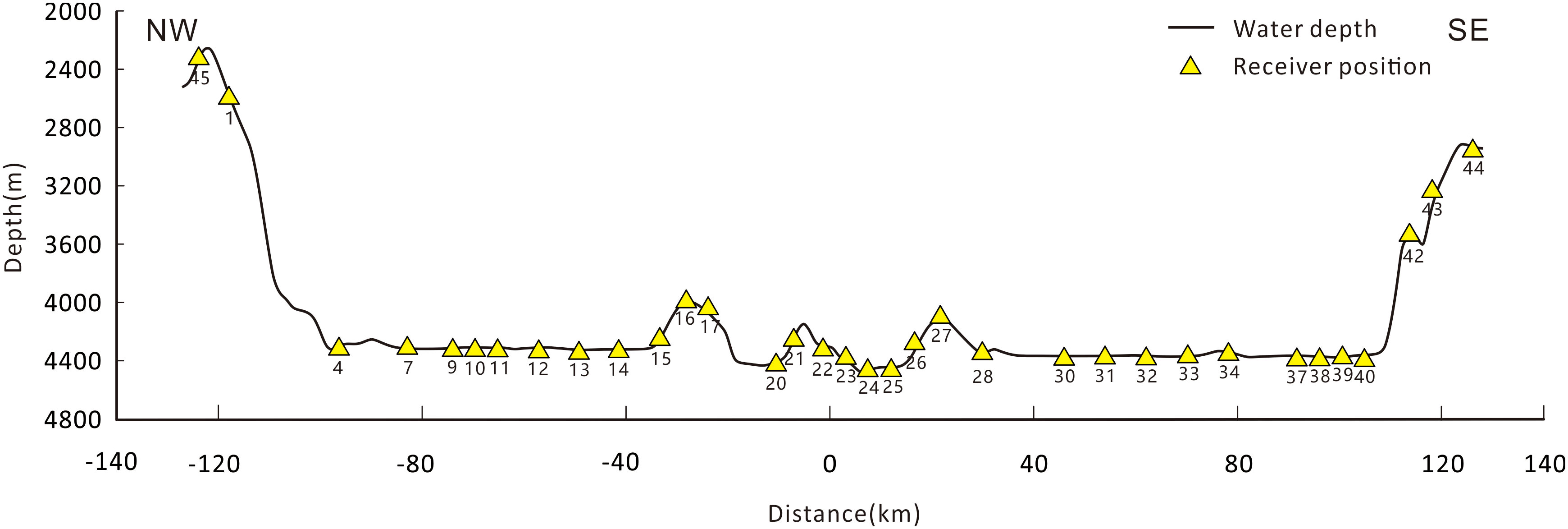
Figure 2 Bathymetry and electromagnetic acquisition geometry.
The spacing of approximately 5 kilometers between stations ensures the accuracy of resistivity imaging of the lithosphere. In general, the majority of Ocean Bottom Electromagnetic (OBEM) stations provided high-quality data. However, we had to exclude data from nine OBEMs (stations 2, 3, 5, 6, 8, 18, 19, 29, 35,36,41and 46) due to issues such as poor electrode connections or a lack/failure of compass on the instruments. Despite this, we were able to obtain high-quality Magnetotelluric (MT) responses with periods ranging from approximately 50 to 10,000 seconds. The shortest period limit was set to 50 seconds for shallow OBEMs and 200 seconds for deep-water OBEMs. Figure 3 shows the time domain plots of the MT receiver measurements.

Figure 3 Time-domain plots of the MT receiver measurements.
The survey conducted in this study covered water depths ranging from 3,000 to 4,500 meters. Considering the shielding effect of seawater on natural-source electromagnetic signals, we started truncating the data from 200 seconds to 500 seconds period for the Magnetotelluric (MT) analysis. Additionally, there was noticeable noise caused by ocean currents on the left side of the profile during deployment. To minimize the impact of this noise, we made the decision to start truncating the data from approximately 500 seconds period onwards.
We conducted dimensionality analysis using the open-source software MTpy (Kirkby et al., 2019) and visualized the data with MTpy. In Figure 4, the phase tensor ellipse section illustrates the ellipticity and tilt values of the 33 measurement points. The lower impedance tilt to the east of the mid-ocean ridge is consistent with the primary 2D conductivity structure beneath the ridge. However, on the left side of the phase tensor profile, as well as at measurement points MT17 to MT21, there is a noticeable departure from 2D behavior in the period range of 100-1000s, with erratic ellipse azimuths. This suggests the presence of some 3D conductivity effects in these areas, likely caused by nearby steep bathymetry/topography variations and the inhomogeneity of the deep asthenosphere.
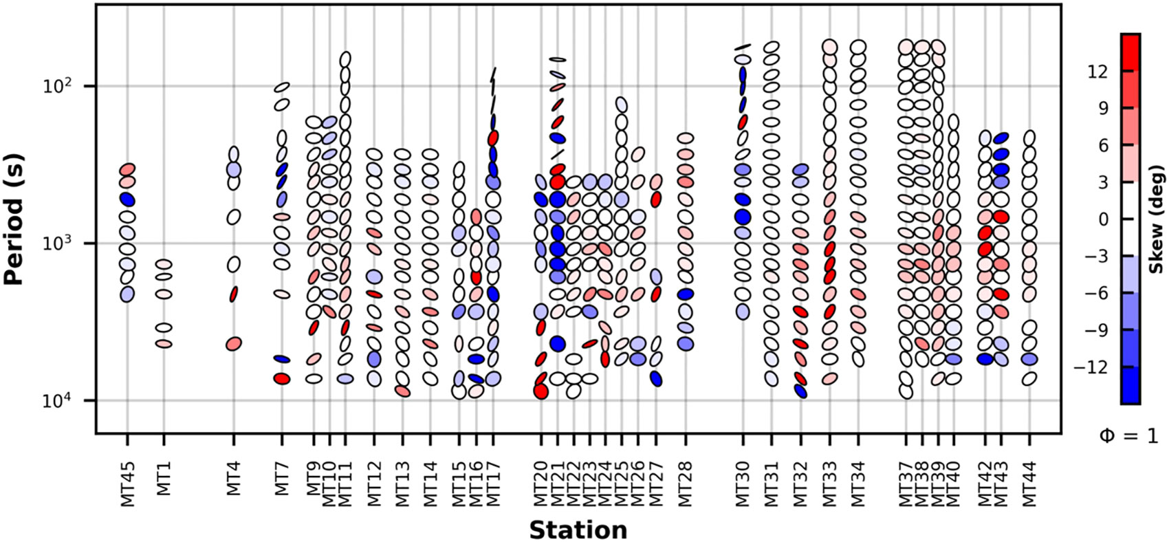
Figure 4 Phase tensor analysis plot for the 34 measurement point.
Due to the challenges in accurately fitting the phases caused by the 3D nature of the data, we made the decision not to include the TE mode data from data points 7, 15, 16, 43, 21, 30 and 43, as well as the TM mode data from data point 17 during the inversion process. The changes observed in the long-period data trend could be attributed to variations in deep structures or the influence of mantle olivine anisotropy. It is important to acknowledge that the 2D determinant inversion method employed in this study has limitations when dealing with complex 3D structures. In such cases, a 3D inversion would be more appropriate. However, in this particular study, the effectiveness of a 3D inversion was not satisfactory due to the presence of only one profile.
We employ the open-source software MARE2DEM for inversion, which utilizes an adaptive finite element algorithm for forward modeling (Key, 2016). The objective of the inversion is to seek a refined underground resistivity model that can effectively interpret the measured data while accounting for data uncertainty. The inversion program we utilize follows an Occam-type inversion scheme, enabling the estimation of three-axis anisotropic resistivity (Constable et al., 1987; Berdichevsky and Dmitriev, 2008).
In this study, the x-direction aligns with the axis of the oceanic ridge, the y-direction is perpendicular to the ridge, and the z-direction points downwards. To ensure the inversion is not influenced by the structure in the input starting model, we initialized the inversion with a uniform halfspace model of 10Ωm. The model dimensions for this inversion cover a range of 2000 km×2000 km in the y and z directions, which adequately encompasses the cross-sectional length (approximately 260 km). The model cells are smaller (around 5 km) in the core region and coarser in the outer part of the cross-section. As shown in the Figure 5, the inversion process utilizes three unknown resistivity tensor elements on 7895 triangular cells, extending from the seafloor to the mantle. Smaller cells are suitable for representing rugged seafloor features, while larger cells are used to model deeper regions. In total, there are 23685 unknown parameters.
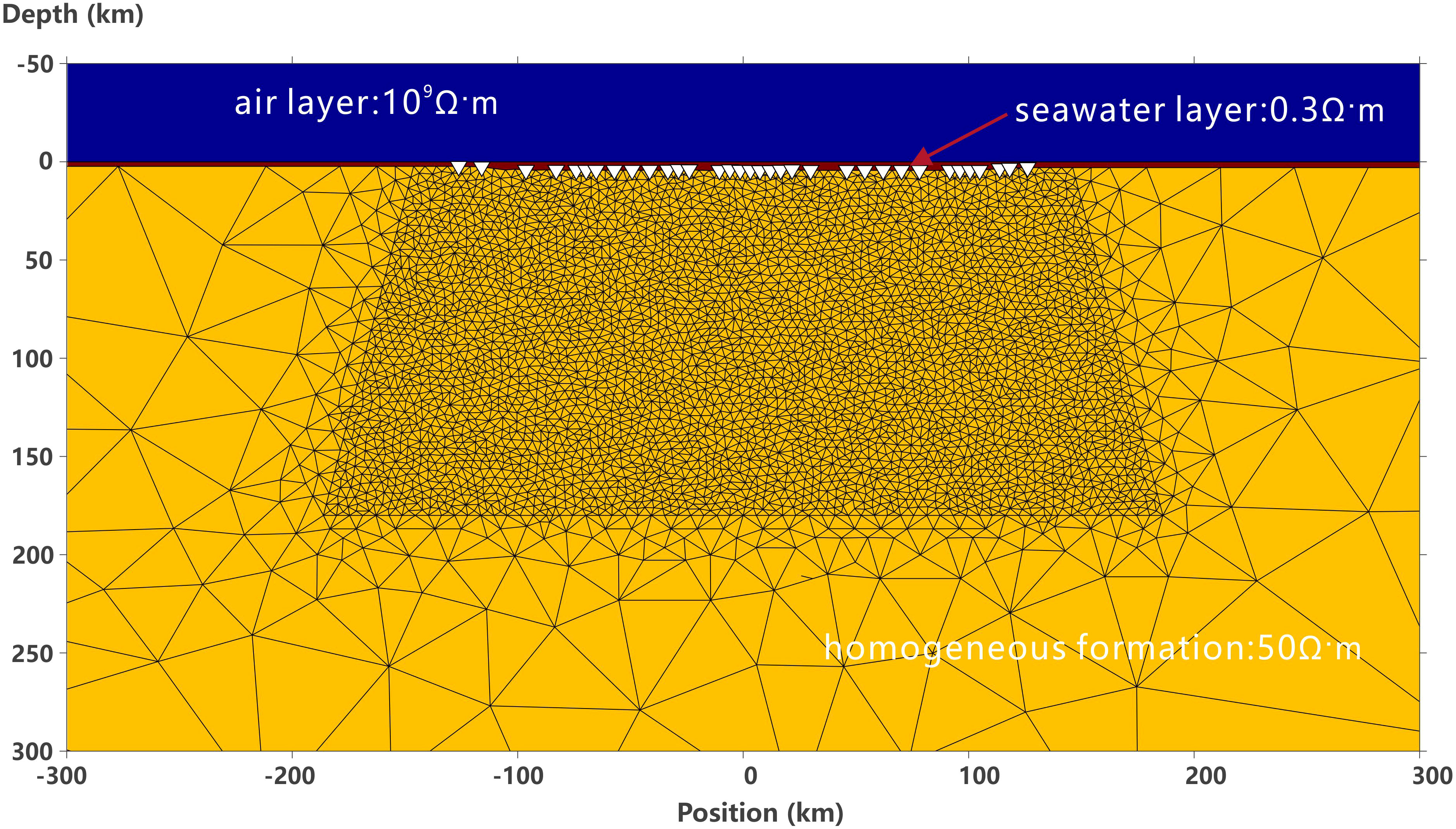
Figure 5 Mesh partition of the initial model.
Enhanced by the general Occam method, the inversion actively minimizes the following function:
where m is the n dimensional vector of model parameters with units log10(resistivity). Matrix R is the roughness operator.The first term represents the model’s roughness, indicating how smooth or jagged it is. the second term is the fit of model’s forward response F(m) to the observed data vector d weighted by the data’s inverse standard errors in the diagonal matrix W. F represents the forward modeling operator, which is based on the Euclidean norm. Occam’s method employs an automatic search to determine the best combination of parameters that balances the fit to the data and the smoothness of the model. In the case of considering three-axis anisotropic resistivity, the model’s roughness term is expanded to
The first three terms measure the spatial roughness of each component of the anisotropic resistivity by evaluating the differences between adjacent resistivity parameters. These terms measure the smoothness or variability of the resistivity distribution in different directions. On the other hand, the last three terms quantify the degree of anisotropy within each cell. These terms help to capture the variations and complexities of anisotropic conductivity within the model. It is important to note that the inversion process only introduces anisotropic conductivity when it is required to accurately fit the observed data.
Equation3 has a unified implicit weighting between measuring spatial roughness and anisotropic roughness, which means that both aspects are given equal priority during the inversion process. This ensures that both spatial roughness and anisotropic roughness are appropriately considered and balanced when generating the final model.
The initial root mean square (rms) for the inversion is 10.1. The lower limits for the errors in apparent resistivity and phase are defined as 10% and 2.85°, respectively.These error limits have proven effective for the data, resulting in a fitting misfit of 2.36. To avoid overfitting and ensure a more balanced inversion, we restart the inversion process with a slightly higher target fitting misfit, approximately 10% higher at 2.6. This adjustment helps to ensure that the data is not overly fitted, striking a balance between accurately fitting the data and avoiding excessive complexity in the model MT data and model responses are shown in the Figure 6.
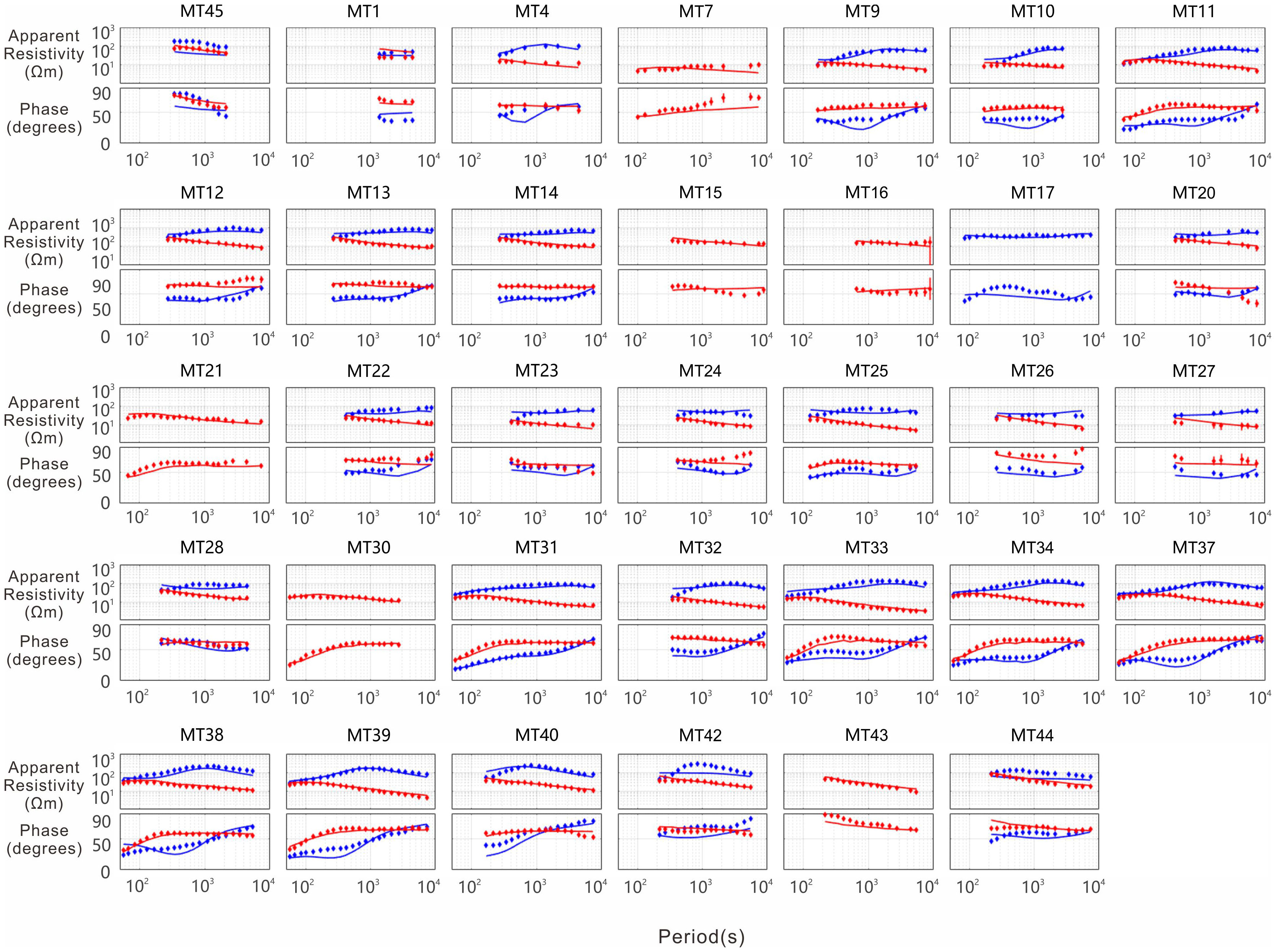
Figure 6 MT data and model responses are shown. The apparent resistivity is measured in ohm-m, and the phase is measured in degrees. The TE mode data is represented by blue symbols, while the TM mode data is represented by red symbols. The solid lines correspond to the responses of the best-fitting model. The station names are clearly displayed above each panel.
Analysis of results
The inversion results, as shown in Figure 7, present a profile displaying the distribution of electrical structures beneath the inactive mid-ocean ridge in the southwestern sub-basin of the South China Sea. In this inversion model, four significant features are observed.
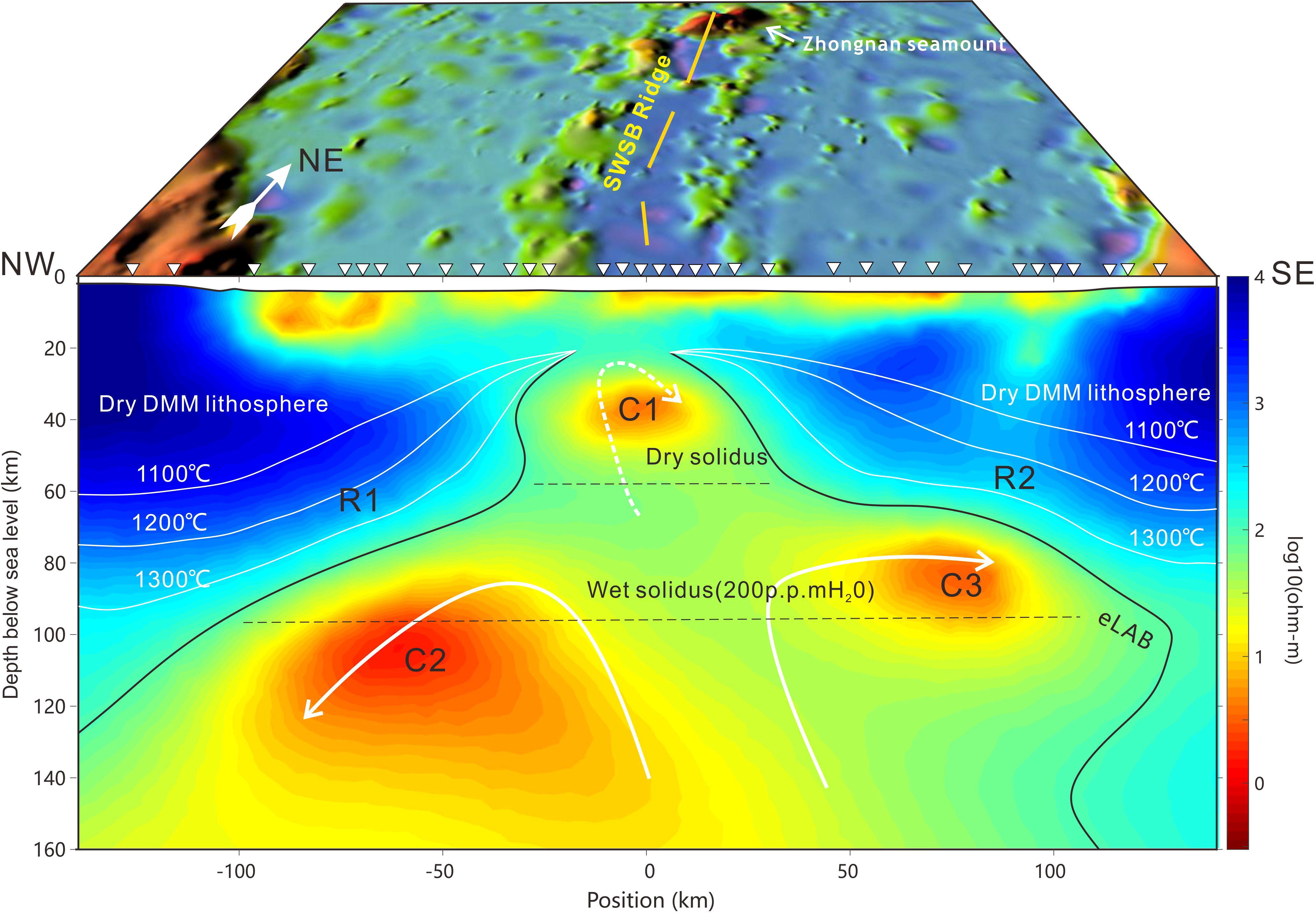
Figure 7 Marine magnetotelluric resistivity imaging of the southwestern sub-basin of the South China Sea. The profile extends to a depth of 160 km. On the profile, the resistivity colors represent the logarithmic resistivity (in Ohm-meter) in the vertical direction obtained from the non-linear inversion of data from seafloor magnetotelluric stations (indicated by white triangles on the seafloor). The color scale presents the electrical resistivity in log10[ρ(Ωm)]. Blue to red colors indicate high conductivity to low resistivity, possibly due to the presence of partial melt. The contour at approximately 100 Ωm is interpreted as the base of the electrical lithosphere according to Johansen et al. (2019). Outside and above the eLAB, a distinct transition is observed, characterized by an increase in resistivity of the olivine-rich rocks without melt. We assume that the temperature of the lithosphere below a depth of 15 km beneath the seafloor is similar to a half-space cooling model, and the measured values agree with the SE03 conductivity and temperature model. The predicted isotherms are shown as white lines, calculated based on the SE03 model. The dry and 200 parts per million H2O solidi for peridotite are sourced from Hirschmann et al. (2009).
The first feature indicates that the melt ascent channel is blocked beneath the stalled mid-ocean ridge. As a result, the molten material descends and accumulates, forming a small melt trap at depths of 20-40 kilometers (C1) with a resistivity of approximately 9 Ohm-meter. This region appears as a small low-resistivity zone, possibly indicating the enrichment of melt formed by mantle upwelling.The second feature reveals significant low-resistivity anomalies (C2) along the northwest survey line of the oceanic ridge, with resistivity values of approximately 1 Ohm-meter. These anomalies are distributed between 80 and 160 kilometers and are likely supplied by deeper sources of molten material. The low-resistivity anomalies in region C2 exhibit the largest extent and deeper depths.The third feature shows relatively smaller low-resistivity anomalies (~2 Ohm-meter) along the southeast survey line of the oceanic ridge (C3). These anomalies are possibly associated with small-scale heat cycles occurring in the area.The fourth feature indicates that the imaged lithospheric lid has a thickness ranging from 20 to 90 kilometers with resistivity values greater than or equal to 100 Ohm-meter. Moreover, this thickness shows a positive correlation with the age of the lithosphere (R1, R2).
These findings suggest that following the cessation of seafloor spreading at mid-ocean ridges, partial melt continues to persist. The magnetotelluric profile of the ocean basin reflects the thermal-electric structure beneath the southwestern sub-basin of the South China Sea at this moment.
Model appraisal is a critical step in the inversion process. In the presented model, the influence of anisotropy is generally negligible, except for the shallow left side of the mid-ocean ridge, where the vertical conductivity exhibits the highest values (Figure 8). However, it is important to consider that the selection of anisotropic factors during the inversion process (Baba et al., 2006) may have contributed to this observation. During the inversion, a aniso.penatly weight of a=1 was employed to account for anisotropy.
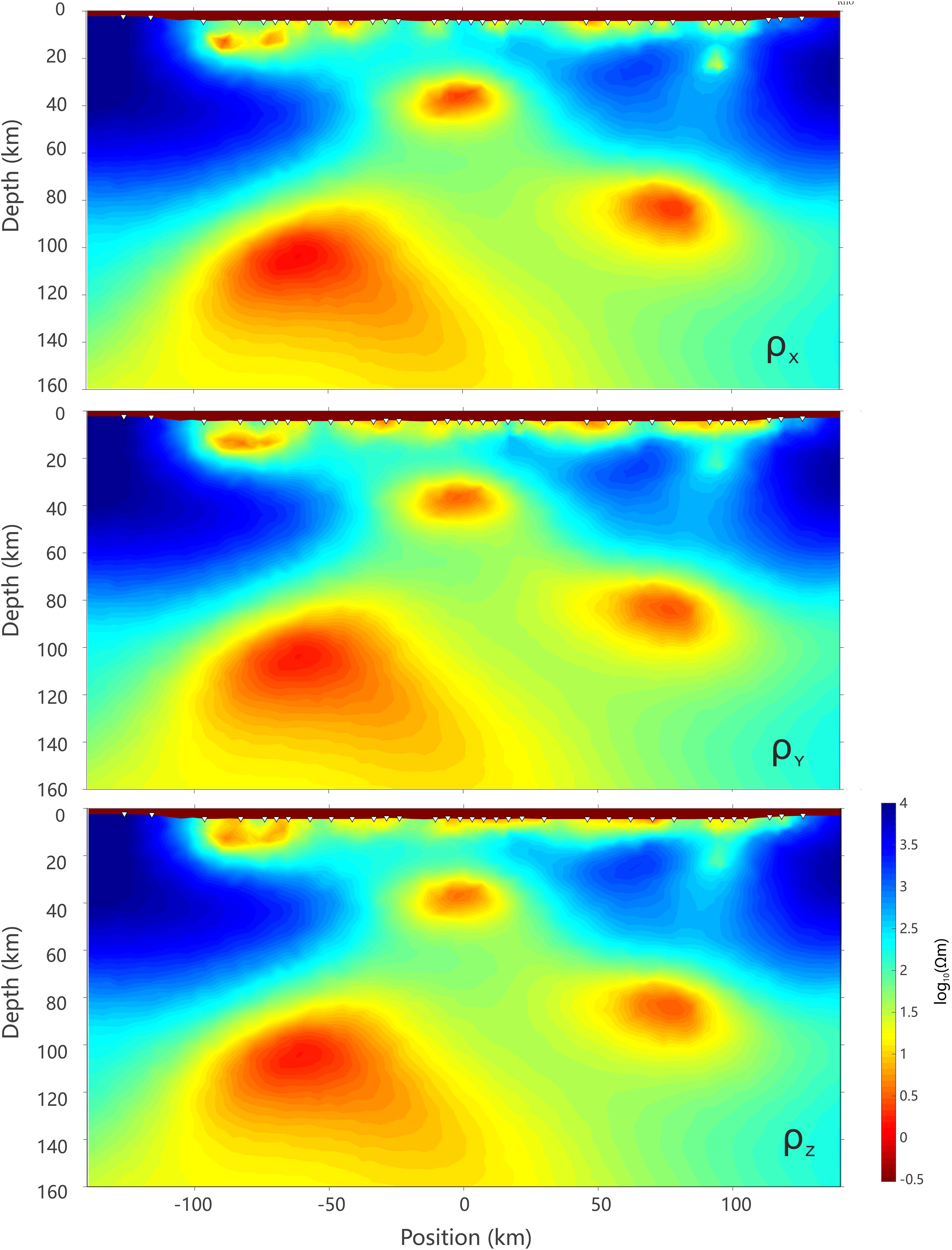
Figure 8 The anisotropic resistivity obtained from the two-dimensional inversion of TE+TM mode data.
We also conducted sensitivity tests on the MT response to important model features, particularly in high conductivity areas. We varied the resistivity of the conductors in rectangular regions A, B, and C to make them more resistive and observed the changes in overall RMS data misfit for forward modeling tests. The resistivity of these conductors ranged from 1-9 Ωm, and for the sensitivity tests, we increased it to 100 Ωm in regions A, B, and C. Figure 9 shows the increase in RMS data misfit for each test. As shown in Figure 10, removing shallow conductor A resulted in a 10% increase in misfit for the TE mode and a 6% increase for the TM mode. Removing deep conductor B resulted in a 26% increase in misfit for the TE mode. Removing vertical conductor C resulted in a 20% increase in misfit for the TE mode. These test results confirm the sensitivity of our data to features A, B, and C, with perturbing these features significantly increasing the local data misfit. As expected, the data is more sensitive to anomalies B and C. Matsuno et al. (2012) found that conductors located at depths of 6-60 km in the ocean only affect MT responses below 1,000 seconds. Due to data noise and other issues, we had to remove some data within 1,000 seconds from MT stations constraining region A, but the high conductivity region A still has some reliability. These test results emphasize the importance of each conductor in fitting the data.
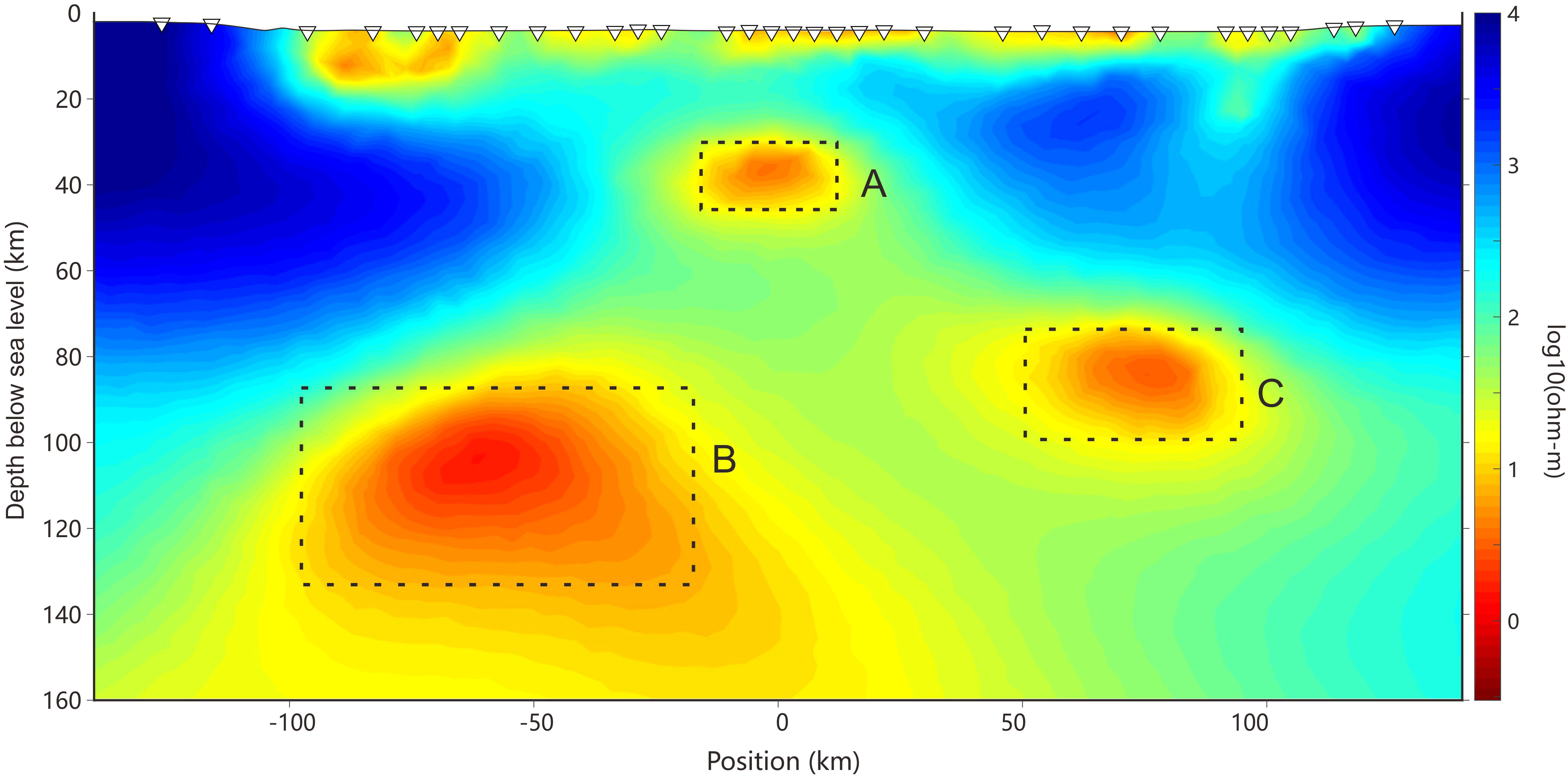
Figure 9 Model sensitivity test regions.The data sensitivity of the three main conductors in regions (A–C) was obtained by replacing them with a uniform resistivity of 100 Ωm and calculating the resulting MT response.
Discussion
This asymmetric and discontinuous conductive area is significantly different from the symmetric triangular conductor observed in mid-ocean ridge spreading systems (e.g., Key et al., 2013). These conductive regions likely outline the thermal structure and decompression melting area beneath the upwelling mantle magma during the process of back-arc rollback. The highly conductive zones beneath the mid-ocean ridge may be one of the reasons for the intense modification of the crust by post-rift magmatism in the southwestern sub-basin of the South China Sea (Evans et al., 2005; Caricchi et al., 2011). When interpreting the 2D conductivity profiles through the oceanic lithosphere (Figure 6), various factors such as temperature, pressure, rock type, grain size, water permeability, melt content, and dehydration reactions of hydrous minerals must be taken into account (Hacker et al., 2003; Ni et al., 2011). Dry peridotite, basalt, gabbro, and other minerals are the main components of the mantle material. Factors such as their melting ratio, content, and water content can all affect the electrical resistivity properties of the mantle (Caricchi et al., 2011). Additionally, the content and effects of H2O and CO2 in the melt should also be considered (Wallace and Green, 1988; Sifré et al., 2014; Green and Liebermann, 1976).
We have selected three vertical profiles, A, B, and C, passing through the centers of high conductivity anomalies on the northwest, vertical, and southeast sides of the profile, respectively. Figure 10 illustrates the specific locations of these three vertical profiles, A, B, and C, along the profile line. The relationship between temperature and depth for each profile, A, B, and C, is depicted in Figure 11A. In Figure 11A, the measured conductivity is inverted using the SEO3 model to obtain the corresponding temperatures, which are represented by blue lines. Additionally, the geothermal gradient calculated using the half-space cooling model is shown in red. Figure 11B presents the calculated profiles of partial melting content and their associated water content. These profiles provide valuable insights into the thermal and electrical properties of the mantle.

Figure 10 The sensitivity test results are shown as the increase in the RMS data fit for the TE and TM mode data subsets for regions (A–C).
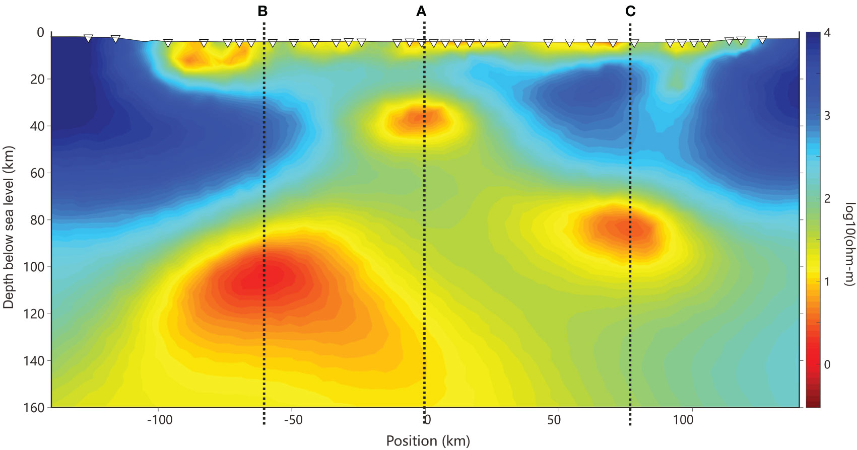
Figure 11 The three vertical profiles (A-C) selected along the profile line.
For profile A, the depth of the conductive region in the upper part is approximately 40km. The melt depth of profile B is between 90km and 140km, while the high conductivity region of profile C is within the depth range of 60-80km. These are definitely not explainable by melting of a CO2-free H2O-depleted mantle, since too high temperatures and/or too high melt contents are demanded (Presnall and Gudfinnsson, 2005; Naif et al., 2013).For example, at a temperature of approximately 1350°C, the resistivity of dry olivine without melt is ≥102Ωm (Constable et al., 1992; Constable, 2006; Yoshino et al., 2009; Gardés et al., 2014). This resistivity value is much higher than that of shallow conductors. Shallow conductors may include silicates (basaltic melt) (e.g., Sifré et al., 2014) and conductive components such as water (e.g., Wang et al., 2006; Pommier et al., 2008; Green et al., 2010; Figure 12B). For profiles A, B, and C, if the melt content in the high conductivity region is not too high (2%-4%), which would cause buoyant mantle upwelling (Hier-Majumder and Courtier, 2011; Faul, 2001), a water content of around 4.0wt% is required, especially for the high conductor in profile B, which needs a higher percentage of water. Considering that the high conductivity region C1 is located beneath a mid-ocean ridge, the presence of melt that can be hydrated can explain its low resistivity value. We have not considered the influence of CO2 on the observed resistivity. Carbonate melt is expected in the deep mantle beneath spreading ridges (Cartigny et al., 2008; Dasgupta et al., 2013), so the low resistivity of profile B and C may also be influenced by CO2, with actual water content lower than the calculated values (Dasgupta and Hirschmann, 2010; Marty, 2014). The high conductivity region in profile B has a larger scale and deeper depth, These are definitely not explainable by melting of a CO2-free H2O-depleted mantle, since too high temperatures and/or too high melt contents are demanded (Presnall and Gudfinnsson, 2005; Naif et al., 2013). the presence of two parallel conduction mechanisms: conduction through a covalent polymer-like hydrated silicate melt and ion conduction through carbonate melt. The combined effect of these two mechanisms results in the observed high conductivity in this region (Gaillard et al., 2008; Bialas et al., 2010).
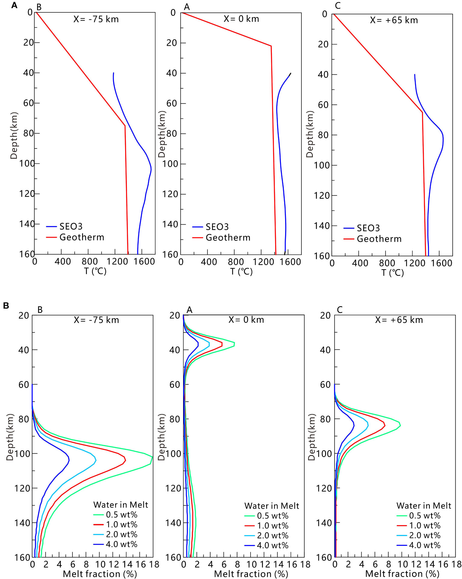
Figure 12 (A) The temperature-depth relationship for profiles A, B, and C is illustrated in Figure 11A. To estimate the melt content and water content of the conductor, we employed the Standard Electrical Olivine 3 (SEO3) model (Constable, 2006) through modeling. The blue lines in Figure 11A represent the maximum temperature, obtained by inverting the measured conductivities to SEO3. These temperatures are then combined with the red line, which represents the geotherm calculated using the half-space cooling model. (B) Figure 11B presents the water content in the melt versus depth, as well as the calculated melt content, for profiles A, B, and C.
Conclusion
This study presents an electrical section of the southwestern sub-basin of the South China Sea, obtained from a large-scale MT array, revealing that the sub-basin has ceased spreading and extends down to a depth of 160km beneath the mid-ocean ridge. Based on our electrical model and joint interpretation, the following conclusions can be drawn:
(1) The thickness of the imaged lithospheric lid (>100Ωm) varies between 20 and 90 km and shows a positive correlation with its age. This suggests that the older the lithosphere, the thicker the lithospheric lid.
(2) The melt ascent channel is closed beneath the stalled mid-ocean ridge, causing the melt to fall back and accumulate to form a small melt trap below the inactive ridge. This indicates that the melt is unable to reach the surface due to the closure of the ascent channel.
(3) The presence of a certain proportion of CO2 and H2O in the shallow melt reservoirs and deep depleted mantle beneath the southwestern sub-basin is necessary to create a high conductivity zone and inhibit upwelling at this depth. This implies that the presence of CO2 and H2O affects the conductivity and prevents buoyant upwelling in the region.
Subsequent studies can integrate the analysis of seismic wave velocity and petrophysical sampling in the southwestern sub-basin of the South China Sea to provide a more accurate understanding and insight into the material cycling and geological processes within the Earth’s interior. Combining different methods of analysis can further enhance our understanding of the dynamics and processes occurring in the sub-basin.
Code availability statement
MARE2DEM20 is a parallel adaptive finite element code for two-dimensional forward and inverse modelling for electromagnetic geophysics and was used for data modelling and inversion in this project. MARE2DEM is available for download at http://mare2dem.ucsd.edu/. The MT processing software used in this study are available from ftp://ftp.oce.orst.edu/dist/egbert/EMTF/EMTF.tar.gz and https://code.usgs.gov/ghsc/geomag/emtf/fcu/tree/v4.1.
Data availability statement
The data analyzed in this study is subject to the following licenses/restrictions: The data that support the findings of this study are available from GMGS, but restrictions apply to the availability of these data, which were used under special agreement for the current study. All relevant data are, however, available from the corresponding author upon reasonable request and with the permission of GMGS. Requests to access these datasets should be directed tobGlqaWFucGluZzE0QDEyNi5jb20=.
Author contributions
YG: Writing – original draft. JL: Writing – review & editing. FL: Writing – review & editing. RZ: Writing – review & editing. YZ: Writing – review & editing. ZH: Writing – review & editing.
Funding
The author(s) declare financial support was received for the research, authorship, and/or publication of this article. This study was supported by the China Geological Survey Project under contracts No. DD20201118 and No. DD20230069,the Marine Economic Development in Guangdong Province (Grant Number: GDNRC[2023]40),the China Geological Survey Project under contracts No.DD20221912,Guangdong Provincial Key Laboratory of Geophysical High-resolution Imaging Technology(2022B1212010002), and Shenzhen Science and Technology Program (Grant No. KQTD20170810111725321).
Acknowledgments
Data acquisition were supported by the Guangzhou Marine Geological Survey (GMGS) and China University of Geosciences Beijing(CUGB),funded by the China Geological Survey Project (No. DD20201118 and No. DD20230069). This cruise was conducted onboard R/V “Hai Yang Di Zhi 4” by Guangzhou Marine Geological Survey (GMGS) China.
Conflict of interest
The authors declare that the research was conducted in the absence of any commercial or financial relationships that could be construed as a potential conflict of interest.
Publisher’s note
All claims expressed in this article are solely those of the authors and do not necessarily represent those of their affiliated organizations, or those of the publisher, the editors and the reviewers. Any product that may be evaluated in this article, or claim that may be made by its manufacturer, is not guaranteed or endorsed by the publisher.
References
Baba K., Chave A. D., Evans R. L., Hirth G., Mackie R. L. (2006). Mantle dynamics beneath the East Pacific Rise at 17°S: Insights from the Mantle Electromagnetic and Tomography (MELT) experiment. J. Geophysical Res. 111, B02101. doi: 10.1029/2004JB003598
Barckhausen U., Roeser H. A. (2004). Seafloor spreading anomalies in theSouth China Sea revisited. Continent-Ocean Interact. within East Asian Marg. Seas 149, 121–125. doi: 10.1029/149gm07
Berdichevsky M., Dmitriev V. I. (2008). “Inversion strategy,” in Models and Methods of Magnetotellurics (Springer, Berlin), 453–544. doi: 10.1007/978-3-540-77814-1_12
Bialas R. W., Buck W. R., Qin R. (2010). How much magma is required to rift a continent? Earth Planetary Sci. Lett. 292. doi: 10.1016/j.epsl.2010.01.021
Bown J. W., White R. S. (1994). Variation of oceanic crustal thickness with spreading rate. Earth Planetary Sci. Letters. 121, 435–449. doi: 10.1016/0012-821X(94)90082-5
Briais A., Patriat P., Tapponnier P. (1993). Updated interpretation of magnetic anomalies and seafloor spreading stages in the South China Sea:Implications for the Tertiary tectonics of Southeast Asia. J. Geophysical Res. 98, 6299–6328. doi: 10.1029/92JB02280
Caricchi L., Gaillard F., Mecklenburgh J., Trong E. L. (2011). Experimental determination of electrical conductivity during deformation of melt-bearing olivine aggregates: Implications for electrical anisotropy in the oceanic low velocity zone. Earth Planetary Sci. Lett. 302, 81–94. doi: 10.1016/j.epsl.2010.11.041
Cartigny P., Pineau F., Aubaud C., Javoy M. (2008). Towards a consistent mantle carbon flux estimate: Insights from volatile systematics (H2O/Ce, δD, CO2/Nb) in the North Atlantic mantle (14° N and 34° N). Earth Planetary Sci. Lett. 265, 672–685. doi: 10.1016/J.EPSL.2007.11.011
Constable S. (2006). SEO3: A new model of olivine electrical conductivity. Geophysical J. Int. 166, 435–437. doi: 10.1111/j.1365-246X.2006.03041.x
Constable S., Parker R. L., Constable C. G. (1987). Occam's inversion; a practical algorithm for generating smooth models from electromagnetic sounding data. Geophysics 52, 289–300. doi: 10.1190/1.1442303
Constable S., Shankland T. J., Duba A. (1992). The electrical conductivity of an isotropic olivine mantle. J. Geophysical Res. 97 (B3), 3397–3404. doi: 10.1029/91JB02453
Dalton C. A., Langmuir C. H., Gale A. (2014). Geophysical and geochemical evidence for deep temperature variations beneath mid-ocean ridges. Science 344 (6179), 80–83. doi: 10.1126/science.1249466
Dasgupta R., Hirschmann M. M. (2010). The deep carbon cycle and melting in Earth's interior. Earth Planetary Sci. Lett. 298, 1–13. doi: 10.1016/J.EPSL.2010.06.039
Dasgupta R., Mallik A., Tsuno K., Withers A. C., Hirth G., Hirschmann M. M. (2013). Carbon-dioxide-rich silicate melt in the Earth’s upper mantle. Nature 493, 211–215. doi: 10.1038/nature11731
Dunn R. A., Martinez F. (2011). Contrasting crustal production and rapid mantle transitions beneath back-arc ridges. Nature 469, 198–202. doi: 10.1038/nature09690
Egbert G. D. (1997). Robust multiple-station magnetotelluric data processing. Geophysical J. Int. 130, 475–496. doi: 10.1111/J.1365-246X.1997.TB05663.X
Evans R. L., Hirth G., Baba K., Forsyth D., Chave A., Mackie R. (2005). Geophysical evidence from the MELT area for compositional controls on oceanic plates. Nature 437, 249–252. doi: 10.1038/nature04014
Faul U. H. (2001). Melt retention and segregation beneath mid-ocean ridges. Nature 410, 920–923. doi: 10.1038/35073556
Forsyth D. W. (1992). “Geophysical constraints on mantle flow and melt generation beneath mid-ocean ridges,” in Mantle flow and melt generation at mid-ocean ridges. Geophysical Monograph Series, vol. 71 . Eds. Morgan J. P., Blackman D. K., Sinton J. M. (American Geophysical Union), 183–280.
Forsyth D. W., Chave A. D. (1994). Experiment investigates magma in the mantle beneath mid-ocean ridges. Eos, Trans. Am. Geophysical Union 75, 537–540. doi: 10.1029/94EO02023
Franke D., Barckhausen U., Baristeas N., Engels M., Ladage S., Lutz R., et al. (2010). The continent-ocean transition at the southeastern margin of the South China Sea. Mar. Petroleum Geology 28, 1187–1204. doi: 10.1016/J.MARPETGEO.2011.01.004
Franke D., Savva D., Pubellier M., Steuer S., Mouly B., Auxietre J.-L., et al. (2014). The final rifting evolution in the South China Sea. Marine and Petroleum Geology 58 (2014), 704–720. doi: 10.1016/j.marpetgeo.2013.11.020
Gaillard F., Malki M., Iacono-Marziano G., Pichavant M., Scaillet B. (2008). Carbonatite melts and electrical conductivity in the asthenosphere. Science 322, 1363–1365. doi: 10.1126/science.1164446
Gardés E., Gaillard F., Tarits P. (2014). Toward a unified hydrous olivine electrical conductivity law. Geochemistry, Geophysics, Geosystems 15, 4984–5000. doi: 10.1002/2014GC005496
Green D. H., Liebermann R. C. (1976). Phase equilibria and elastic properties of a pyrolite model for the oceanic upper mantle. Tectonophysics 32, 61–92. doi: 10.1016/0040-1951(76)90086-X
Green D. H., Hibberson W. O., Kovács I. J., Rosenthal A. (2010). Water and its influence on the lithosphere–asthenosphere boundary. Nature 467, 448–451. doi: 10.1038/nature09369
Hacker B. R., Abers G. A., Peacock S. M. (2003). Subduction factory, 1, Theoretical mineralogy, densities, seismic wave speeds, and H2O contents. J. Geophysical Res. 108 (B1), 2029. doi: 10.1029/2001JB001127
Hier-Majumder S., Courtier A. M. (2011). Seismic signature of small melt fraction atop the transition zone. Earth Planetary Sci. Lett. 308. doi: 10.1016/J.EPSL.2011.05.055
Hirschmann M. M., Tenner T., Aubaud C., Withers A. C. (2009). Dehydration melting of nominally anhydrous mantle: The primacy of partitioning. Phys. Earth Planetary Interiors 176, 54–68. doi: 10.1016/J.PEPI.2009.04.001
Huang H., Qiu X., Zhang J., Hao T. (2019). Low-velocity layers in the northwestern margin of the South China Sea: Evidence from receiver functions of ocean-bottom seismometer data. J. Asian Earth Sci. 186, 104090. doi: 10.1016/j.jseaes.2019.104090
Johansen S. E., Panzner M., Mittet R., Amundsen H. E., Lim A., Vik E., et al. (2019). Deep electrical imaging of the ultraslow-spreading Mohns Ridge. Nature 567, 379–383. doi: 10.1038/s41586-019-1010-0
Jokat W., Ritzmann O., Schmidt-Aursch M. C., Drachev S., Gauger S., Snow J. (2003). Geophysical evidence for reduced melt production on the Arctic ultraslow Gakkel mid-ocean ridge. Nature 423, 962–965. doi: 10.1038/nature01706
Key K. (2016). MARE2DEM: a 2-D inversion code for controlled-source electromagnetic and magnetotelluric data. Geophysical J. Int. 207, 571–588. doi: 10.1093/GJI/GGW290
Key K., Constable S. (2002). Broadband marine MT exploration of the East Pacific Rise at 9°50′N. Geophysical Res. Lett. 29. doi: 10.1029/2002GL016035
Key K., Constable S., Liu L., Pommier A. (2013). Electrical image of passive mantle upwelling beneath the northern East Pacific Rise. Nature 495, 499–502. doi: 10.1038/nature11932
Kirkby A., Zhang F., Peacock J. R., Hassan R., Duan J. (2019). The MTPy software package for magnetotelluric data analysis and visualisation. J. Open Source Software 4, 1358. doi: 10.21105/JOSS.01358
Li C., Xu X., Lin J., Sun Z., Zhu J., Yao Y., et al. (2014). Ages and magnetic structures of the South China Sea constrained by deep tow magnetic surveys and IODP Expedition 349. Geochemistry 15, 4958–4983. doi: 10.1002/2014GC005567
Li C., Zhou Z., Li J., Hao H., Geng J. (2007). Structures of the northeasternmost South China Sea continental margin and ocean basin: geophysical constraints and tectonic implications. Mar. Geophysical Res. 28, 59–79. doi: 10.1007/S11001-007-9014-9
Macdonald K. C., Scheirer D. S., Carbotte S. M. (1991). Mid-ocean ridges: Discontinuities, segments and giant cracks. Science 253 (5023), 986–994. doi: 10.1126/science.253.5023.986
Marty B. (2014). The origins and concentrations of water, carbon, nitrogen and noble gases on Earth. Earth Planetary Sci. Lett. 313, 56–66. doi: 10.1016/j.epsl.2011.10.040
Matsuno T., Evans R. L., Seama N., Chave A. D. (2012). Electromagnetic constraints on a melt region beneath the central Mariana back-arc spreading ridge. Geochemistry Geophysics Geosystems 13 (10), 10017. doi: 10.1029/2012GC004326
Matsuno T., Seama N., Shindo H., Nogi Y., Okino K. (2022). Enhanced and asymmetric melting beneath the southern mariana back-arc spreading center under the influence of pacific plate subduction. J. Geophysical Research: Solid Earth 127. doi: 10.1029/2021JB022374
McKenzie D., Jackson J., Priestley K. (2005). Thermal structure of oceanic and continental lithosphere. Earth Planetary Sci. Lett. 233, 337–349. doi: 10.1016/J.EPSL.2005.02.005
Naif S., Key K., Constable S., Evans R. L. (2013). Melt-rich channel observed at the lithosphere–asthenosphere boundary. Nature 495, 356–359. doi: 10.1038/nature11939
Ni H., Keppler H., Behrens H. (2011). Electrical conductivity of hydrous basaltic melts: implications for partial melting in the upper mantle. Contributions to Mineralogy Petrology 162, 637–650. doi: 10.1007/S00410-011-0617-4
Nolasco R., Tarits P., Filloux J. H., Chave A. D. (1998). Magnetotelluric imaging of the Society Islands hotspot. J. Geophysical Res. 103, 30287–30309. doi: 10.1029/98JB02129
Peace A. L., Welford J. K., Geng M., Sandeman H. A., Gaetz B. D., Ryan S. S. (2018). Rift-related magmatism on magma-poor margins: Structural and potential-field analyses of the Mesozoic Notre Dame Bay intrusions, Newfoundland, Canada and their link to North Atlantic Opening. Tectonophysics 745, 24–45. doi: 10.1016/J.TECTO.2018.07.025
Pin Y., Di Z., Zhao-shu L. (2001). A crustal structure profile across the northern continental margin of the South China Sea. Tectonophysics 338, 1–21. doi: 10.1016/S0040-1951(01)00062-2
Pommier A., Gaillard F., Pichavant M., Scaillet B. (2008). Laboratory measurements of electrical conductivities of hydrous and dry Mount Vesuvius melts under pressure. J. Geophysical Res. 113, B05205. doi: 10.1029/2007JB005269
Presnall D. C., Gudfinnsson G. H. (2005). Carbonate-rich melts in the oceanic low-velocity zone and deep mantle. doi: 10.1130/0-8137-2388-4.207
Reid I. D., Jackson H. R. (1981). Oceanic spreading rate and crustal thickness. Mar. Geophysical Res. 5, 165–172. doi: 10.1007/BF00163477
Qiu Y., Chen G. N., Liu F. L., Peng Z. L. (2008). Discovery of granite and its tectonic significance in southwestern basin of the South China Sea. Geological Bulletin of China (in Chinese with English Abstract) 27 (12), 2104–2107. doi: 10.3969/j.issn.1671-2552.2008.12.017
Schlindwein V., Schmid F. (2016). Mid-ocean-ridge seismicity reveals extreme types of ocean lithosphere. Nature 535, 276–279. doi: 10.1038/nature18277
Sifré D., Gardes E., Massuyeau M., Hashim L., Hier-Majumder S., Gaillard F. (2014). The electrical conductivity during incipient melting in the oceanic low velocity zone. Nature 509, 81–85. doi: 10.1038/nature13245
Song X. X., Li C. F., Yao Y. J., Shi H. S. (2017). Magmatism in the evolution of the South China Sea: Geophysical characterization. Marine Geology 394 (2017), 4–15. doi: 10.1016/j.margeo.2017.07.021
Stern T., Henrys S. A., Okaya D. A., Louie J. N., Savage M. K., Lamb S., et al. (2015). A seismic reflection image for the base of a tectonic plate. Nature 518, 85–88. doi: 10.1038/nature14146
Taylor B., Hayes D. E. (1983). Origin and history of the South China Sea basin. The tectonic and geologic evolution of Southeast Asian seas and islands, Vol. 27, 23–56. doi: 10.1029/GM027p0023
Tozer B. L., Sandwell D. T., Smith W. H., Olson C. J., Beale J., Wessel P. (2019). Global bathymetry and topography at 15 arc sec: SRTM15+. Earth Space Sci. 6, 1847–1864. doi: 10.1029/2019EA000658
Wallace M. E., Green D. H. (1988). An experimental determination of primary carbonatite magma composition. Nature 335, 343–346. doi: 10.1038/335343A0
Wang D., Mookherjee M., Xu Y., Karato S. (2006). The effect of water on the electrical conductivity of olivine. Nature 443, 977–980. doi: 10.1038/nature05256
Worzewski T., Jegen M. D., Kopp H., Brasse H., Castillo W. T. (2011). Magnetotelluric image of the fluid cycle in the Costa Rican subduction zone. Nat. Geosci. 4, 108–111. doi: 10.1038/NGEO1041
Xu Y., Wei J., Qiu H., Zhang H., Huang X. (2012). Opening and evolution of the South China Sea constrained by studies on volcanic rocks: Preliminary results and a research design Vol. 57 (Chinese Science Bulletin), 3150–3164. doi: 10.1007/S11434-011-4921-1
Yan Q., Shi X., Castillo P. R. (2014). The late Mesozoic–Cenozoic tectonic evolution of the South China Sea: A petrologic perspective. J. Asian Earth Sci. 85, 178–201. doi: 10.1016/J.JSEAES.2014.02.005
Yoshino T., Matsuzaki T., Shatskiy A., Katsura T. (2009). The effect of water on the electrical conductivity of olivine aggregates and its implications for the electrical structure of the upper mantle. Earth Planetary Sci. Lett. 288, 291–300. doi: 10.1016/j.epsl.2009.09.032
Yoshino T., Mcisaac E., Laumonier M., Katsura T. (2012). Electrical conductivity of partial molten carbonate peridotite. Phys. Earth Planetary Interiors 194, 1–9. doi: 10.1016/J.PEPI.2012.01.005
Yu M., Yan Y., Huang C., Zhang X., Tian Z., Chen W., et al. (2018). Opening of the South China sea and upwelling of the hainan plume. Geophysical Res. Lett. 45, 2600–2609. doi: 10.1002/2017GL076872
Zhang G., Luo Q., Zhao J., Jackson M. G., Guo L., Zhong L. (2018). Geochemical nature of sub-ridge mantle and opening dynamics of the South China Sea. Earth Planetary Sci. Lett. 489, 145–155. doi: 10.1016/J.EPSL.2018.02.040
Zhang Q., Wu S., Dong D. (2016). Cenozoic magmatism in the northern continental margin of the South China Sea: evidence from seismic profiles. Mar. Geophysical Res. 37, 71–94. doi: 10.1007/s11001-016-9266-3
Zhao M., Qiu X., Xia S., Xu H., Wang P., Wang T. K., et al. (2010). Seismic structure in the northeastern South China Sea: S-wave velocity and Vp/Vs ratios derived from three-component OBS data. Tectonophysics 480, 183–197. doi: 10.1016/J.TECTO.2009.10.004
Zhou H., Dick H. J. (2013). Thin crust as evidence for depleted mantle supporting the Marion Rise. Nature 494, 195–200. doi: 10.1038/nature11842
Keywords: marine magnetotelluric (MT), mantle structure, the South China Sea, extinct oceanic ridge, deep electrical imaging
Citation: Gao Y, Li J, Li F, Zhang R, Zhao Y and He Z (2023) Deep electrical imaging of the extinct oceanic ridge in the southwestern sub-basin of the South China Sea. Front. Mar. Sci. 10:1270778. doi: 10.3389/fmars.2023.1270778
Received: 01 August 2023; Accepted: 20 October 2023;
Published: 17 November 2023.
Edited by:
Xingsen Guo, University College London, United KingdomReviewed by:
Yaoguo Li, Colorado School of Mines, United StatesHongzhu Cai, China University of Geosciences Wuhan, China
Copyright © 2023 Gao, Li, Li, Zhang, Zhao and He. This is an open-access article distributed under the terms of the Creative Commons Attribution License (CC BY). The use, distribution or reproduction in other forums is permitted, provided the original author(s) and the copyright owner(s) are credited and that the original publication in this journal is cited, in accordance with accepted academic practice. No use, distribution or reproduction is permitted which does not comply with these terms.
*Correspondence: Jianping Li, bGlqaWFucGluZzE0QDEyNi5jb20=; Fuyuan Li, bGVlZnV5dWFuQHNpbmEuY29t