 Fabio Bozzeda1,2†
 Leonardo Ortega3†
 Leonardo Lopes Costa4
 Lucia Fanini1
 Carlos A. M. Barboza5Anton McLachlan6
 Omar Defeo7*†
- 1Department of Biological and Environmental Sciences and Technologies (DiSTeBA), University of Salento, Lecce, Italy
- 2National Biodiversity Future Center (NBFC), Palermo, Italy
- 3Departamento de Biología Poblacional, Dirección Nacional de Recursos Acuáticos, Montevideo, Uruguay
- 4Laboratório de Ciências Ambientais, Universidade Estadual do Norte Fluminense Darcy Ribeiro, Campos dos Goytacazes, Rio de Janeiro, Brazil
- 5Nucleo em Ecologia e Desenvolvimento, Instituto de Biodiversidade e Sustentabilidade NUPEM, Universidade Federal do Rio de Janeiro, Macae, Rio de Janeiro, Brazil
- 6Retired, Jeffrey's Bay, South Africa
- 7Laboratorio de Ciencias del Mar, Facultad de Ciencias, UNDECIMAR, Montevideo, Uruguay
Beach erosion is a complex process influenced by multiple factors operating at different spatial scales. Local (e.g., waves, tides, grain size, beach width and coastal development) and regional (e.g., sea level rise and mean sea level pressure) factors both shape erosion processes. A comprehensive understanding of how these drivers collectively impact sandy beach erosion is needed. To address this on a global-scale we assembled a database with in-situ information on key physical variables from 315 sandy beaches covering a wide morphodynamic range and complemented by satellite data on regional variables. Our results revealed the combined influence of local and regional factors on beach erosion rates. Primary drivers were regional anomalies in mean sea level pressure and variations in mean sea level, and local factors such as tide range, beach slope and width, and Dean’s parameter. By analyzing morphodynamic characteristics, we identified five distinct clusters of sandy beaches ranging from wave-dominated microtidal reflective beaches to tide-modified ultradissipative beaches. This energy dissipation gradient emerged as a critical factor, with erosion rates increasing with beach width and dissipativeness. Our study also highlighted the tangible impact of climate change on beach erosion patterns. Hotspots were identified, where intensification of regional anomalies in mean sea level pressure, increasing onshore winds and warming rates, and rising sea levels synergistically accelerated erosion rates. However, local variables were found to either amplify the effects of regional factors on erosion or enhance a beach’s resistance, mitigating erosive trends initiated by regional drivers. Our analysis showed that more than one-fifth of the analyzed beaches are experiencing intense, extreme, or severe erosion rates, and highlighted the significant role of human activities in explaining erosion trends, particularly in microtidal reflective and intermediate beaches. This underscores the long-term threat of coastal squeeze faced by sandy beaches worldwide and emphasizes the need to consider both local and regional drivers in order to understand erosion processes. Integrating localized measurements with broader satellite observations is required for a comprehensive understanding of the main drivers behind coastal evolution, which in turn is needed to manage and preserve these fragile ecosystems that are at risk.
Introduction
The sandy beaches that fringe much of the world’s oceans provide varied ecosystem services that are critical in maintaining safe and healthy environments for people. These services include filtering seawater, recycling nutrients, harboring iconic species, providing a highly prized recreation venue and, most importantly, protecting the hinterland by buffering erosion impacts from sea-level rise and storms (Harris and Defeo, 2022). However, because these services are being compromised globally by various stressors, sandy beaches are under strain worldwide (Vousdoukas et al., 2020; Defeo et al., 2021). Yet beaches do not stand alone: they are the fulcrum in the centre of the sandy littoral, flanked by surf zones seaward and dunes landward, and tightly coupled with both through sand exchange. Thus, damage to any one of these closely linked compartments affects all three (McLachlan and Defeo, 2018).
Declines in beach ecosystem service supply have been attributed to a plethora of pressures that impinge from both the landward and seaward sides (Defeo et al., 2009; Defeo et al., 2021; Harris and Defeo, 2022; Rodil et al., 2022). Anthropogenic factors, particularly the exponentially increasing rates of urban development and supporting infrastructure, impair the capacity of beaches to provide coastal protection. In addition, climate change threatens beaches through sea level rise and associated storminess and flooding events (Woodruff et al., 2013), which cause erosion, beach retreat landwards and coastal overtopping (McLachlan and Defeo, 2018; Mentaschi et al., 2018a; Almar et al., 2021). These contrasting forces cause coastal squeeze, constricting sandy beaches between encroaching urban and industrial development from land and sea-level rise from the ocean (McLachlan and Defeo, 2018; McLachlan and Defeo, 2023). This ‘press-press’ compound perturbation is responsible for substantial long-term losses of sandy beach ecosystem services and the goods and benefits that they provide (e.g., food, recreation, coastal protection), benefits which have been documented worldwide (Harris and Defeo, 2022). Coastal squeeze also interacts with other pulse or press perturbations to impact sandy shores, producing unpredictable synergistic effects on the social-ecological system (Costa et al., 2020; Fanini et al., 2020; Defeo and Elliott, 2021; Corte et al., 2022; Costa et al., 2022).
Beach sand provides an essential buffer against sea level rise and extreme weather events and, therefore, protection against coastal erosion (Harris and Defeo, 2022). However, the balance between the supply of, and demand for, this ecosystem service is not always sustainable: as for other sandy ecosystems, beach and dune sands have been mined to extract minerals for a variety of purposes, notably construction (Bendixen et al., 2019; UNEP, 2019; Torres et al., 2021; Bisht, 2022; UNEP, 2022). The United Nations has raised awareness of the crisis of global sand loss to construction, totaling 50 billion tons per year and mainly related to population increase and urbanization (UNEP, 2019; UNEP, 2022). Beaches are increasingly sand-starved due to these sand-mining practices and dune removal, further aggravated by artificial hardened structures alongshore (e.g., concrete groins, seawalls, revetments and breakwaters), all contributing to reduced sand supply and ensuing erosion and shoreline retreat (Mentaschi et al., 2018a; Defeo et al., 2021). This deficit of sand aggravates the coastal squeeze phenomenon, related erosional processes and coastal hazards. The sand deficit also has significant economic impacts because the unit used to estimate the value of available surface for seaside activities is square meters of sand (Fanini et al., 2021 and references therein).
Recent work has revealed a worrying global scenario concerning sand beach erosion patterns. Luijendijk et al. (2018) assessed shoreline change rates for the period 1984–2016 using satellite images and found 24% of the world’s sandy beaches to be eroding at rates exceeding 0.5 m·yr-1. Moreover, Vousdoukas et al. (2020) showed that coastal recession, driven by sea-level rise, could result in a loss of almost half of the world’s sandy beaches by the end of the century. However, sea-level rise is not the only climate-related putative factor affecting sandy beach erosion (Brooks, 2020). For example, the projected increasing frequency of extreme El Niño and La Niña events over the twenty-first century could lead to extreme coastal erosion and flooding on opposite sides of the Pacific Ocean basin, independent of sea-level rise (Barnard et al., 2015). The combination of press (e.g., increasing sea surface temperature, sea-level rise) and pulse (e.g., El Niño, heatwaves, hurricanes) climate perturbations have compound effects (sensu Zscheischler et al., 2018) that have triggered interacting physical processes at multiple spatial and temporal scales, leading to unprecedented impacts on sandy shores.
Long-term field data also show considerable between-beach variation in erosion rates, even for adjoining beaches, highlighting the need to undertake erosion studies and predictions at a local level (Short, 2022 and references therein). Indeed, climate-related stressors, in combination with other regional and local factors, will determine when and how each beach responds to these pressures (Defeo et al., 2021; Short, 2022). As mentioned before, among several relevant local factors of anthropogenic origin, increasing urban development and supporting infrastructure, particularly for coastal recreation and tourism, have had deleterious ecological and socioeconomic consequences for sandy beaches (Fanini et al., 2020; Defeo et al., 2021). In addition, recent global meta-analyses and spatially intensive studies have revealed that the effects of these co-occurring stressors, associated with urbanization and beach overuse, interact with local beach conditions (e.g., beach slope, grain size, expressed as morphodynamics) to yield specific responses in each beach system (Costa et al., 2020; Corte et al., 2022; Costa et al., 2022).
The foregoing evidence highlights the role of multiple local and seascape drivers in impacting beach dynamics. Yet, little is known about how these multiple co-occurring anthropogenic, atmospheric and climatic drivers interact with local habitat conditions (i.e., beach morphodynamics) to affect beach susceptibility to erosion processes. Here we assemble an unprecedented dataset of in situ local quantitative information on beach properties (e.g., grain size, slope, Dean’s parameter) for hundreds of sandy beaches worldwide, complemented by satellite information on relevant physical, atmospheric and urbanization variables. We use this dataset to unravel the contributions of local and regional factors in beach erosion patterns. Specifically, we ask whether local or large-scale factors, or their interaction, could be the main explanatory variables for sandy beach erosion. In addition, we assess whether local omit characteristics related to beach morphodynamics play a role as explanatory factors in worldwide trends in beach erosion.
Methods
Defining sandy beaches
Sandy shores comprise three contiguous and connected systems: the foredunes, beach and surf zone (Harris and Defeo, 2022). Among these zones there are constant exchanges of nutrients, biota and, above all, sand, such that they are considered to be a single geomorphic unit called the Littoral Active Zone (LAZ, McLachlan and Defeo, 2018). Within the LAZ, different beach morphodynamic types arise from the interplay between tides, waves and sand grain size. These range from wave-dominated, narrow, steep, reflective beaches with coarse-grained sand and surf zones minimal or absent, through a series of intermediate forms, to tide-modified ultradissipative beaches that are wide and low gradient with extensive surf zones and fine-grained sand, where waves and tides both play important roles (McLachlan et al., 2018; Jackson and Short, 2020). Beyond the tide-modified beach types, shores are even wider and lower gradient and are referred to as tide-dominated sand flats. Following Harris and Defeo (2022), we limited the scope of this study to sheltered and exposed open-ocean sandy shores of all morphodynamic types, and excluded sandy beaches located in lakes, lagoons, estuaries, and fjords, where sediment deposition dynamics are influenced by additional factors. Moreover, tide-dominated sand flats are not within the scope of this paper.
Database
Our database was assembled with both local (beach specific) and regional information. We captured local information on essential morphodynamic variables from 315 sandy beaches worldwide, based on the information contained in Defeo and McLachlan (2013); Barboza and Defeo (2015); Defeo et al. (2017); Costa et al. (2022), and on new information gathered from published literature. The dataset was constructed using local scale data, referring to beach units, where a beach unit is defined as a continuous stretch of beach that is expected to respond as a system (homogeneously) to external factors. Information was only included in the database if it was explicitly stated in the main text or supplementary material of the original papers. This means that the entire dataset used in this analysis is based on in-situ local data, and does not include local data derived from satellites or estimated figures from graphs.
Beach slope, grain size and tidal range were selected a priori as the key local sandy beach physical variables gathered from the literature, based on: a) paradigms earlier provided by McLachlan and Defeo (2018) (and references therein), and b) their consistent availability throughout all the publications accessed for this work. When information about a specific physical variable was not available in the papers reviewed, an additional bibliographic search for each sandy beach was performed, and/or data were retrieved by direct contact with the authors of the papers. Beaches with substrate classified coarser than ‘sand’ (sensu Blott and Pye, 2001) were excluded a priori from the analysis. Tidal range was locally assessed via the software WXTide (which allows for local corrections) and confirmed for each beach based on the information contained in tide tables for each country (Turiano and Cruz, 2017).
Two compound indices of beach state were included in the database: the Beach Width Index and the dimensionless fall velocity or Dean’s parameter (Ω). The Beach Width Index, which has been used as a proxy for beach width (McLachlan and Defeo, 2018) because it represents the linear distance (in m) from the low- to the high-tide marks, was obtained by dividing the tidal range by the beach slope. Ω values were either taken from the corresponding papers when available, or if information on wave height and period was provided, it was estimated using the formula provided by Short (1999):
where Hb is breaker height (in m), Ws is sand fall velocity (m·s–1) and T is wave period (s). This index of beach state measures how reflective or dissipative a microtidal beach is. Ω values<2 characterize reflective beaches (narrow, with steep slopes and coarse sands) and Ω values >5 define dissipative beaches (wide intertidal, flat beach slopes and fine sands), with values between 2 and 5 indicating intermediate beach states. However, not all the beaches sampled had this variable available in the published articles.
Regional data on sea surface temperature anomalies, mean sea level pressure anomalies, and meridional and zonal winds anomalies were obtained from the IRI/LDEO Climate Data Library Center (http://iridl.ldeo.columbia.edu/expert/SOURCES/.NOAA/: Grumbine, 1996; Kalnay et al., 1996; Cavalieri et al., 1997; May et al., 1998; Reynolds et al., 2007). Thus, zonal, meridional winds and the resulting wind speed vectors, sea surface temperature, and mean sea level pressure refer to anomaly trends. For the sake of simplicity, these variables will be referred to hereafter as sea surface temperature, mean sea level pressure, and meridional and zonal winds, respectively. The spatial resolution of the sea surface temperature grids was 0.25°, while for mean sea level pressure and meridional and zonal winds, it was 2.5°. Global ocean trends in warming, mean sea level pressure, and winds were estimated using a linear model of each annual pixel for 1982 – 2021. The yearly means and long-term linear trends were calculated using the Ingrid Data Analysis Language in the expert mode platform of the IRI map room. The resulting global trends were visualized using Kriging as the gridding method, and wind speed vectors were calculated and plotted using Surfer 23 software based on historical trends of zonal and meridional winds. The mean sea level trend from 1993 to 2022 (Pekel et al., 2016) was obtained from the Copernicus page of Observations Reprocessing (GLOBAL_OMI_SL_regional_trends DOI 10.48670/moi-00238).
The urbanization level surrounding each beach contained in the dataset was estimated by the Human Modification Metric (HMM: Kennedy et al., 2019). HMM is a measure of the degree of human modification across geo-coordinated lands calculated as the per pixel product (HMs) of the spatial extent and the expected intensity of impact across five major groups of human activities: (1) human settlement (population density, built up areas), (2) agriculture (cropland, livestock), (3) transportation (major roads, minor roads, two tracks, railroads), (4) mining and energy production (mining, oil wells, wind turbines), and (5) electrical infrastructure (powerlines, nighttime lights). The final HMM value was calculated as:
This fuzzy sum is a function that assumes that the contribution of a given factor decreases as other stressors co-occur. In this way, the HMM is a continuous parsimonious gradient of modification at landscape scales ranging from 0 to 1 (Kennedy et al., 2019). Since all components (i.e., major groups of human activities) have been considered, n = 5. HMM was estimated based on the median values at different spatial resolution levels (buffers of 100 m, 500 m, and 1000 m). The elements forming the foundation of the fuzzy sum of the HMM index are chosen based on a geographical criterion, at a fixed distance from the centroid of the study area (e.g., HMM100 corresponds to an HMM value within a radius of 100 m from the centroid). Consequently, for each centroid, HMM values calculated for smaller distances are encompassed within the values computed for larger distances.
To determine the erosion rate for each beach in our database, we extracted information on coastline changes over a 32-year period (1984-2016) following Mentaschi et al. (2018a), using the “Global long-term coastline evolution” database (Mentaschi et al., 2018b), which is accessible through the Joint Research Center Data Catalogue. The study utilized the Global Surface Water Explorer (GSWE) database, which analyzed more than 3 million satellite images to track changes in water presence along more than 2 million virtual transects that provided information on the onshore, offshore, and centroid coordinates of the coastline. To estimate erosion rates, we selected transects with centroid coordinates closest to the central coordinates of each beach. The estimated erosion (coastline retreat) or accretion (coastline advancement) values for the 32-year period were standardized to obtain an erosion rate estimate for each beach. All coordinate extraction and data retrieval from the Joint Research Center database were conducted using the R package “terra” (Hijmans et al., 2022).
This dataset allowed for the identification of beaches experiencing different rates of shoreline change as described in Luijendijk et al. (2018). These beaches were categorized into three main groups: accretion (above 0.5 m·yr-1), stability (between -0.5 and 0.5 m·yr-1), and erosion (below -0.5 m·yr-1). In this paper, data was further categorized into different erosion rate levels following the chronic beach erosion classification scheme proposed by Esteves and Finkl (1998) and extended by Luijendijk et al. (2018), to account for extreme erosion levels as follows: weak erosion (between -0.5 and -1.0 m·yr-1), intense erosion (between -1 and -3 m·yr-1), severe erosion (between -3 and -5 m·yr-1), and extreme erosion (greater retreat than -5 m·yr-1). This analysis was performed per cluster identified in our study.
Analytical approach and models
A deconstructive analytical routine was set up to assess the database, starting from the characterization of the entire database to bring out any hidden patterns and the relative dynamics between variables. The analytical routine consists of four main steps: (1) identifying outliers and collinearity relationships between independent variables; (2) identifying clusters in the database by applying a k-means algorithm; (3) assessing the relative contribution of the independent variables through Random Forests for the whole dataset and for the two main clusters identified in step (2); and (4) using Partial Dependence Plots (PDPs) on both the whole dataset to gain a deeper understanding of the dynamic relationships between variables, and within each cluster to identify the key factors that influenced the response variable.
Step 1: The multicollinearity analysis was performed to avoid information redundancy among the independent variables and to obtain the most parsimonious model (Dormann et al., 2012). First, we calculated a correlation matrix based on the Spearman coefficient. Once the most significant correlation values were identified, a multiple regression model was applied to the entire set of independent variables to estimate the parameters R², tolerance, and variance inflation factor (VIF). Tolerance is the reciprocal of R² and indicates the degree of independence of a variable. VIF provides an estimation of how much the variability expressed by tolerance is inflated due to the level of correlation expressed by R², allowing for the identification of multicollinearity among the predictor variables nested in groups in a multivariate database (Craney and Surles, 2002). VIF quantifies the severity of multicollinearity in an ordinary least squares regression analysis and provides an index of the extent of increase in the variance of an estimated regression coefficient due to collinearity. VIF is expressed by:
where i indicates the i-th parameter of an ordinary least squares regression referred to the i-th independent variable and R2i is the coefficient of determination obtained from regressing the independent variable in question on all the other independent variables in the model. The final selection of variables was based on these parameter values. VIF values ≥ 5 were considered as evidence of collinearity. Outliers were detected through the Grubbs method (Kannan and Manoj, 2015).
Step 2: Nested clusters within the database were detected by applying a k-means clustering algorithm. This is an unsupervised learning algorithm that takes an unlabeled dataset as input and divides it into K clusters, repeating the process until the best number of clusters is found, each associated with a centroid (Likas et al., 2003). The algorithm’s main aim is to minimize the sum of distances between a data point and its corresponding cluster centroid. The K value should be predetermined (Hartigan and Wong, 1979). The k-means clustering algorithm performs two main tasks: (1) determining the optimal value for K center points or centroids through an iterative process; and (2) assigning each data point to its closest centroid, creating clusters of data points with shared similarities. The best clustering solution is identified by scoring the inertia and silhouette values. Inertia measures the quality of clustering by calculating the sum of squared distances between each data point and its centroid. A good k-means model has low inertia and a low number of K clusters. The Elbow method was used to identify the optimal K value at which the decrease in inertia slows down (Syakur et al., 2018). The silhouette coefficient or silhouette score in k-means is a measure of similarity within clusters (cohesion) compared to other clusters (separation). The silhouette plot displays a measure of how close each point in one cluster is to points in the neighboring clusters. The silhouette coefficient was calculated as:
where S(i) is the silhouette coefficient of the data point i, a(i) is the average distance between i and all the other data points in the cluster to which i belongs, and b(i) is the average distance from i to all clusters to which i does not belong. The silhouette coefficient of the entire cluster was calculated by:
This metric has a range of [-1, 1], where silhouette coefficients close to +1 suggests that the data point is well-matched to its own cluster and poorly matched to other clusters, indicating a clear separation. A value of 0 indicates that the sample is on or very close to the decision boundary between two neighboring clusters and negative values indicate that samples might have been assigned to the wrong cluster (Rousseeuw, 1987). Therefore, the number of clusters that has the lowest silhouette score indicates the best clustering.
Non-metric multidimensional scaling (NMDS) analysis was conducted to obtain a two-dimensional (2D) representation of Bray–Curtis distances between pairs of beaches. To capture the inherent variability of the database in two dimensions, a conical transformation was applied to the data (Zhang, 1997). This transformation helps reduce the variability of multidimensional databases where no dominant predictor emerges, and the overall variability is determined by a multidimensional gradient (Bland and Altman, 1996). The conical transformation approximates the points in the database to points on the surface of a cone, with parameters based on the values of the variables characterizing the database (Zhang, 1997). After applying the conical transformation, the resulting database, which represented the initial one but with reduced gradient dimensionality, was represented using a normal 2D NMDS. The conical transformation was performed using the MatLab software (Hrdina et al., 2019), and the NMDS was subsequently constructed using the vegan package in R software (Oksanen, 2011).
Step 3: Random Forests were used to assess the relative importance of local and regional variables in determining erosion rates (Liaw and Wiener, 2002; Prasad et al., 2021), using both the entire database and for the main two clusters identified in Step 2. Each forest was created by generating 10,000 regression trees from bootstrap data sampling. The Out-Of-Bag error (OOB: Ramosaj and Pauly, 2019) was used to assess the accuracy of the single variables in describing the erosion rate. The analysis was performed using the ‘extendedForest’ packages for R (https://r-forge.r-project.org/projects/gradientforest). Random Forest modeling was chosen due to the high number of variables considered, which implies potential interactions among them, and could limit the strength of other analytical methods. In addition, Random Forest modeling implies less theoretical constraints than non-machine learning methods, being exploratory rather than a direct test of hypotheses.
Step 4: PDPs were applied to the whole dataset, and for the two main clusters identified previously, to assess the effects of the most relevant regional and local predictor variables already identified by Random Forests on erosion rates (response variable). To this end, the marginal effect of a predictor variable on the response variable was quantified, while holding all other predictors fixed at their average values. Thus, PDPs were useful to define not only the degree of influence of each variable but also the direction of the change (Parr and Wilson, 2021). PDPs are essentially carriers of two important pieces of information: 1) the type of relationship that exists between the target variable and the considered predictors, and 2) on which part of the target variable domain each predictor is active. PDPs do not imply causation but rather associations, and were therefore interpreted in conjunction with the other approaches mentioned here.
Results
The global long-term trends in mean sea level pressure indicate that high-pressure centers are intensifying and shifting towards the poles (Figures 1, S1). During high-pressure systems, wind circulation patterns exhibit clockwise rotation in the northern hemisphere and counterclockwise rotation in the southern hemisphere (Figure 1). In regions like the Western Pacific coast of America and the Southeastern Atlantic, wind directions tend to run parallel to the coastline and are associated with a cooling trend. Additionally, the Tropical Pacific region experiences an offshore wind pattern with a considerable cooling trend. In contrast, onshore winds along the Southwestern Atlantic, Indian Ocean, Caribbean, and Southeast Pacific coasts have the potential to induce warming (Figure 2).
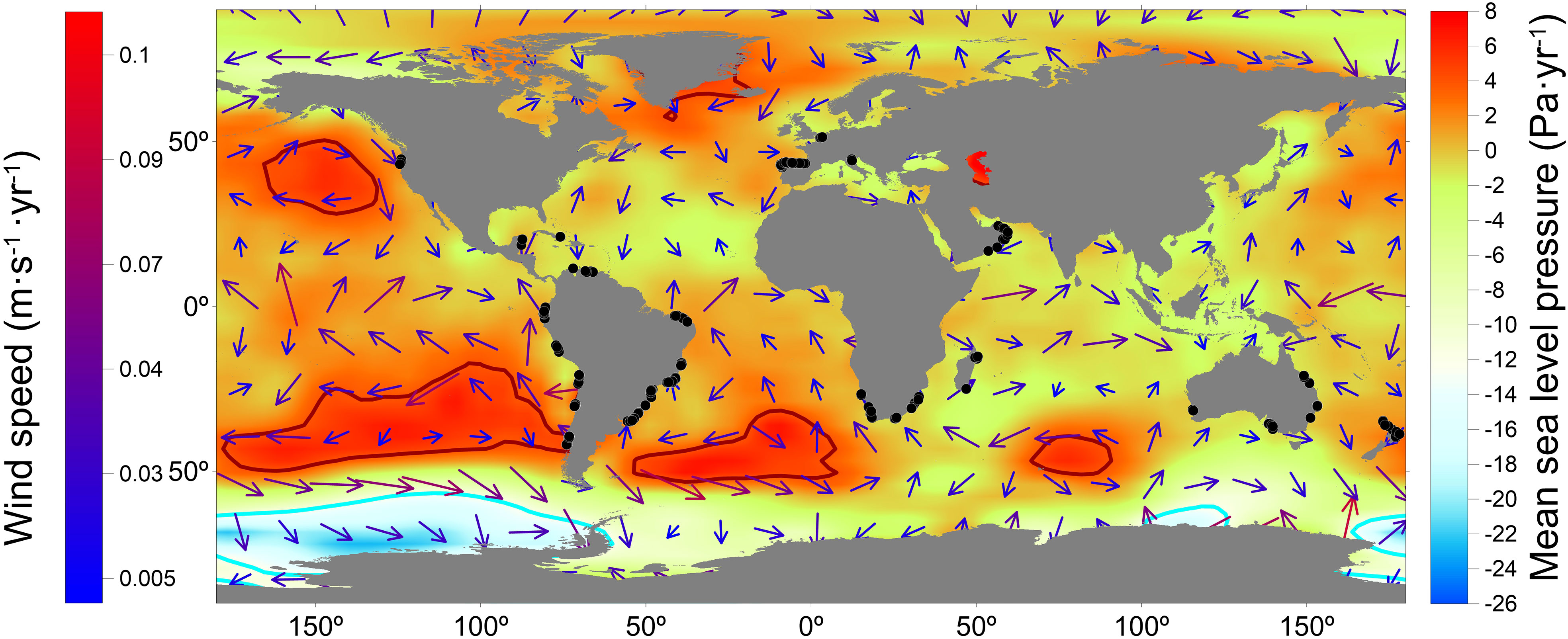
Figure 1 Location of the 315 sandy beaches from five continents included in the analysis (black dots), also showing the global mean sea level pressure anomalies (shading) and wind speed anomalies (arrows) vector trends estimated between 1982 and 2021. The color (see scale on the left) and size of the vectors together correspond to the wind intensity. For simplicity, the Y-axes are labeled as wind speed and mean sea level pressure (see text for details).
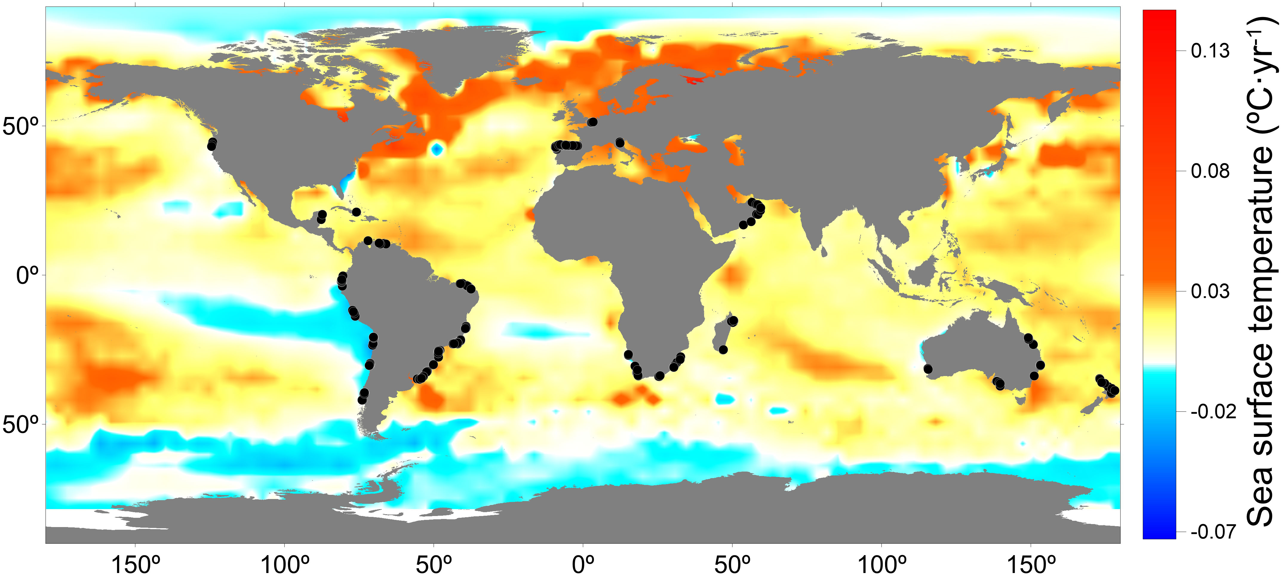
Figure 2 Global sea surface temperature anomalies trends estimated between 1982 and 2021. The color scale shows the increasing rate of warming from blue to red. The location of the 315 sandy beaches from five continents included in the analysis (black dots) is also highlighted. For simplicity, the Y-axis is labeled as sea surface temperature, even though it refers to anomaly trends (see text for details).
Global trends in sea surface temperature display warming hotspots and areas with cooling trends (Figure 2). Although 25% of the beaches included in our database are located in regions experiencing warming hotspots (warming trend > 0.02°C·yr-1), there are a few beaches situated in cooling trend areas, particularly along the South Pacific coast (Figure 2). The regions with warming hotspots roughly align with the areas experiencing the most significant rates of sea level rise (Figure 3).
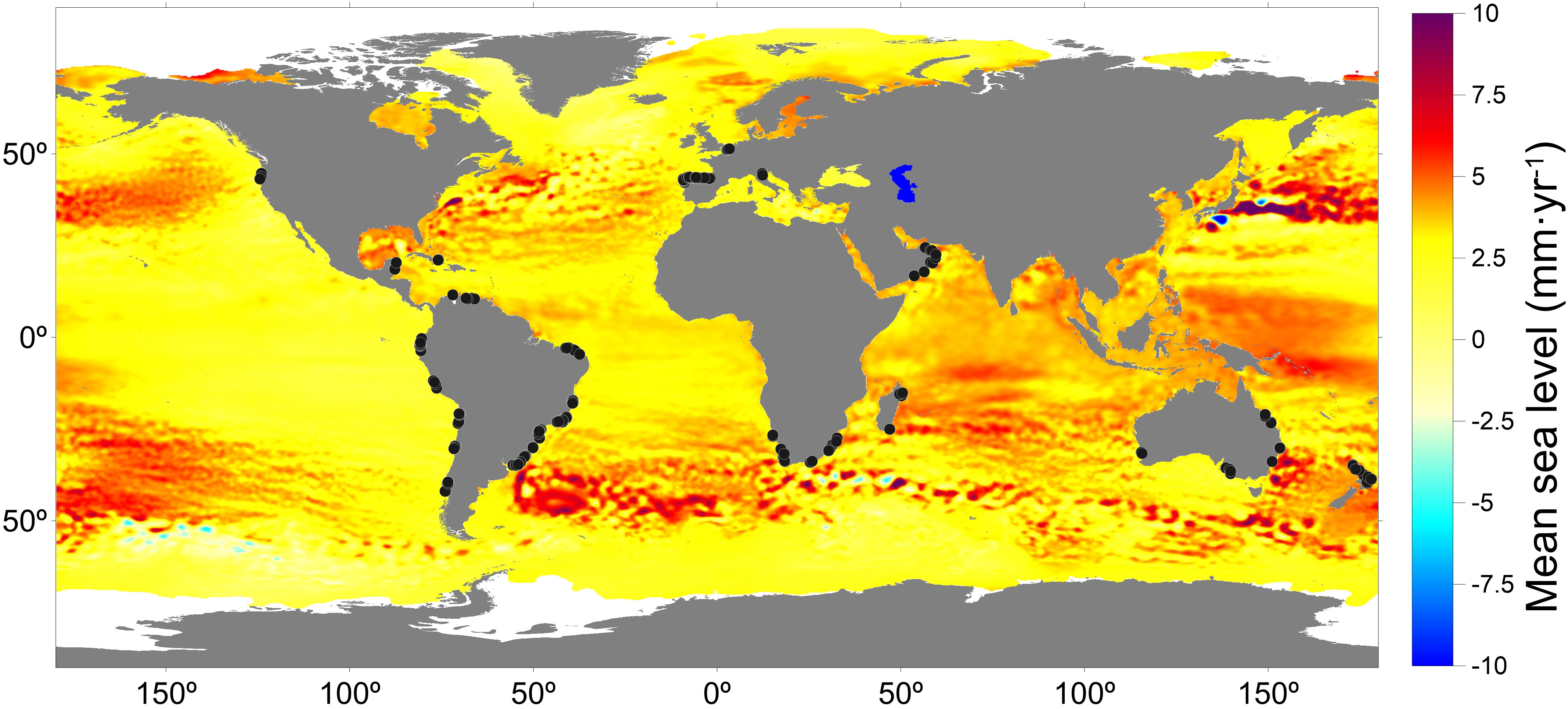
Figure 3 Global mean sea level (MSL) trend map between 1993 and 2021. Source: Observations Reprocessing GLOBAL_OMI_SL_regional_trends DOI 10.48670/moi-00238. The location of the 315 sandy beaches from five continents included in the analysis (black dots) is also highlighted.
The multicollinearity analysis revealed that only the variables HMM100 and HMM500 had VIF values exceeding 5, and these were therefore excluded from the subsequent analysis. The high VIF values were in agreement with R² values > 0.99 and extremely low tolerance values (Tables S1, S2).
The k-means clustering algorithm was applied to the database using a search setting ranging from 2 to 7 clusters. The optimal clustering resulted in 5 asymmetric clusters. The Silhouette score > 0.50 indicates a significant degree of separation between clusters and therefore meaningful and reliable clustering results (Figure S2). Out of the 315 beaches considered, 133 (42%) beaches were grouped in Cluster 1, 108 (34%) in Cluster 2, 51 (16%) in Cluster 3, 21 (7%) in Cluster 4, and 2 (< 1%) in Cluster 5 (Table 1).
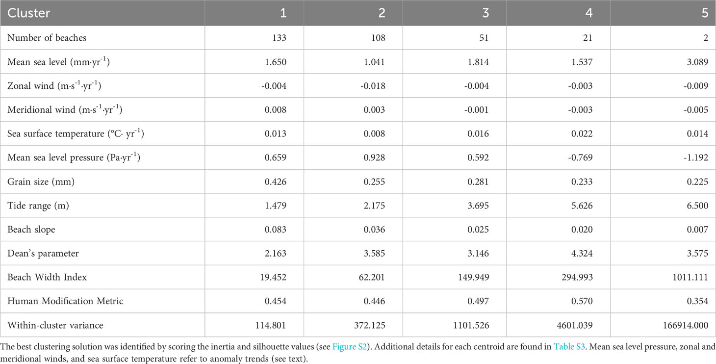
Table 1 Estimated values of the local and regional variables for each centroid of the five clusters obtained by applying a k-means algorithm (see Methods) to the database comprising 315 sandy beaches from five continents.
All variables, except for the zonal wind component, significantly contributed to the k-means clustering (Table 2), indicating the presence of a complex gradient determining the clustering arrangement (Figure 4). A relevant result arising from the relative contribution of local and regional variables in shaping the derived clusters was the notable significance of the local variables in the grouping process (Table 2). The five local variables included in the analysis held the highest statistical relevance in forming the clusters, particularly the Beach Width Index and tide range, followed, in decreasing order of importance, by beach slope, grain size, and the composite Dean’s parameter (Table 2).
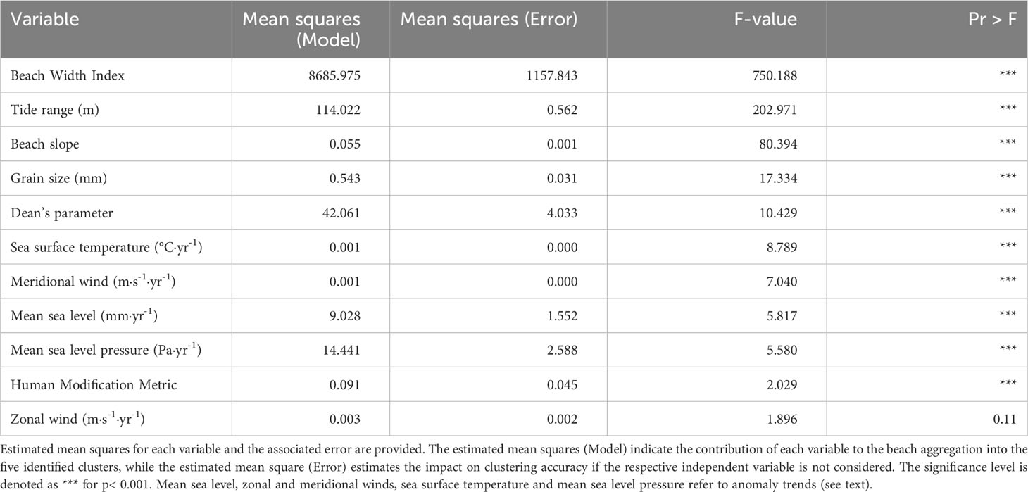
Table 2 ANOVA results for the contribution of local and regional variables (in decreasing order of importance) to the clustering process.
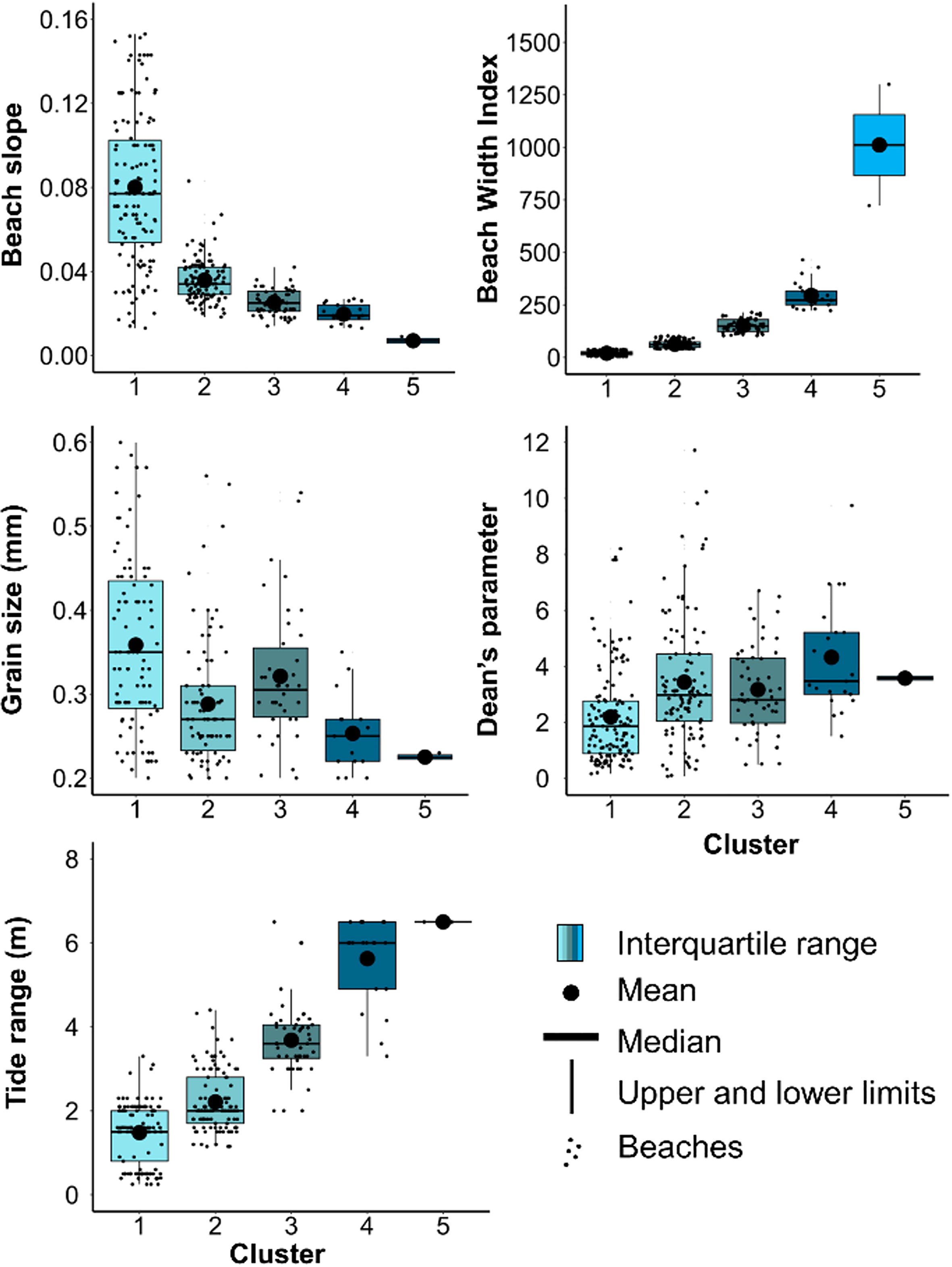
Figure 4 Statistics of relevant local physical and morphodynamic variables (in situ measurements) analyzed for 315 sandy beaches from 5 continents, classified by cluster obtained by applying a k-Means Algorithm (see Table 1 for details). The upper and lower limits correspond to Q3 + 1.5*IQR and Q1-1.5*IQR of the observed variable ranges, respectively.
The values of the local variables, grouped into the 5 clusters obtained from the application of the k-means algorithm, revealed clear patterns that reflected the morphodynamic gradient from microtidal reflective beaches to macrotidal ultradissipative beaches (Table 1; Figure 4). The reflective extreme in Cluster 1 was characterized by steep slopes, coarse grain sizes, and small tide ranges, which were generally below 2 m. These characteristics resulted in narrow beaches with low values of Dean’s parameter. On the other hand, the opposite extreme of the morphodynamic gradient (Cluster 5) was represented by only two ultradissipative beaches characterized by gentle slopes, fine grain sizes, and tidal ranges higher than 4 m, indicating a macrotidal environment. These conditions led to wider beaches with higher values of Dean’s parameter (Table 1; Figure 4). Clusters 2, 3 and 4 denoted intermediate conditions along a continuum of morphodynamic types, exhibiting increasing tide ranges and beach dissipativeness (Figure 4). Specifically, the second cluster primarily consisted of intermediate microtidal beaches, the third cluster comprised predominantly intermediate mesotidal beaches, and the fourth cluster mainly encompassed dissipative macrotidal beaches.
The 2D ordination depicted by the NMDS yielded a reliable depiction of the patterns identified during the clustering process, as evidenced by the low stress value of 0.08 (Figure 5). The five distinct groups were represented by beaches characterized by unique combinations of physical variables that corresponded to distinct morphodynamic environments. These ranged from wave-dominated reflective beaches to tide-modified ultradissipative beaches. The increasing gradient towards beach dissipativeness also corresponded to an increasing gradient in erosion rates, as described below.
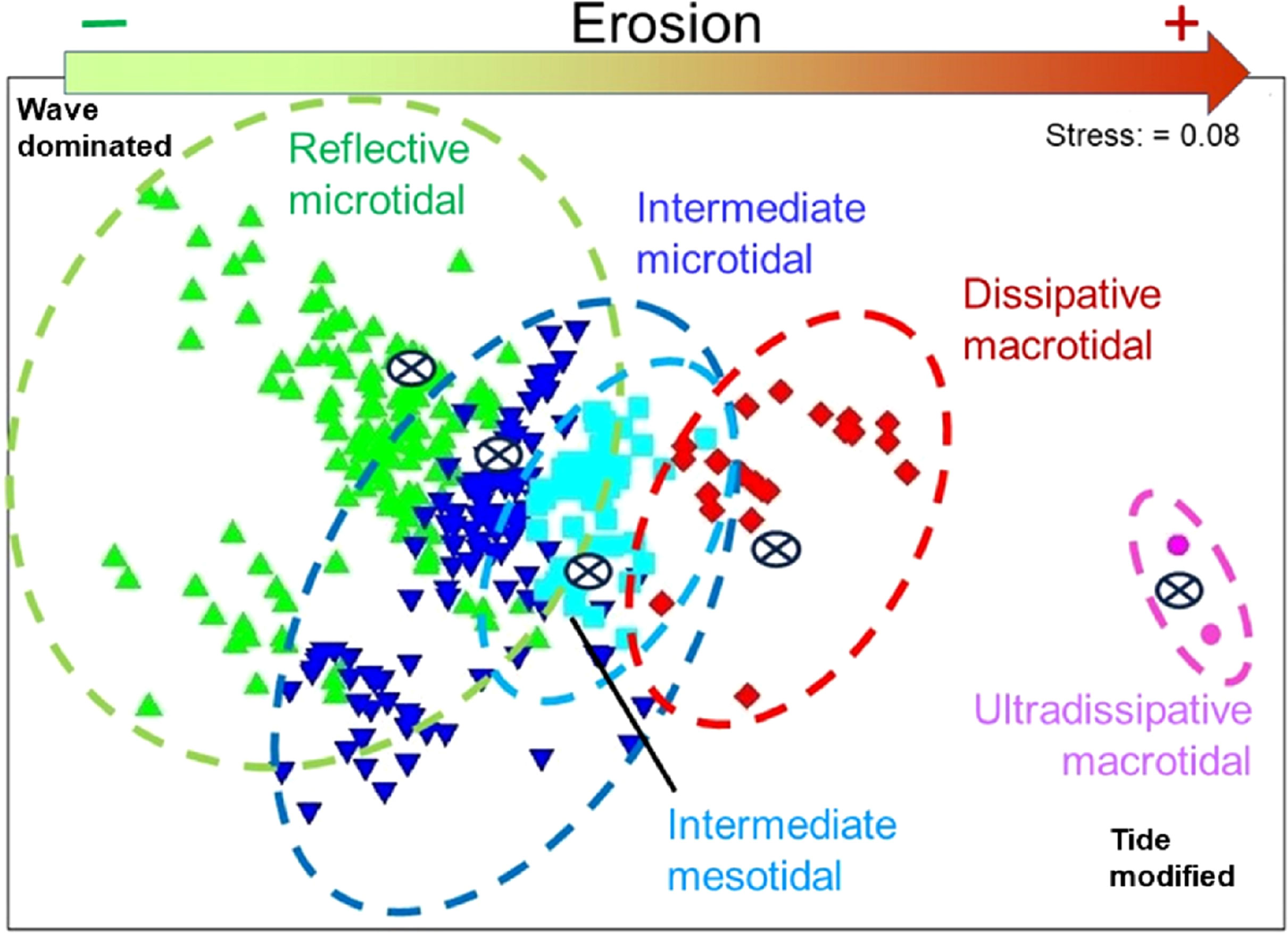
Figure 5 Non-metric Multi-Dimensional Scaling (NMDS) ordination of the 315 sandy beaches from five continents. The values of the local and regional variables were transformed using a conical transformation before calculating the Bray Curtis similarity matrix, which was used to construct the NMDS. The 5 clusters characterized by the k-means algorithm are highlighted with different shapes and colors, along with their respective centroids, and categorized according to their tide ranges and beach morphodynamic characteristics, from tide-dominated to tide-modified beaches (see Table 1). The increasing relative representation of eroded beaches is conceptually depicted (see also Figure 8 and Table 3).
The relative importance of both regional and local variables on erosion rates was assessed by Random Forest analyses (Figure 6). Mean sea level pressure was a critical explanatory driver of worldwide trends, followed in decreasing order of importance by tide range, sea level rise, two compound indices of local beach state (Beach Width Index and Dean’s parameter) and beach slope. An analysis discriminated by cluster revealed a different perspective regarding the relative significance of local and regional variables in depicting erosion trends (Figure 7). In Cluster 1, which represents microtidal reflective conditions, the combined effects of meridional and zonal winds, along with the HMM and mean sea level, emerged as critical drivers in explaining erosion trends. These variables were followed, in descending order of importance, by sea level pressure, Dean’s parameter, grain size and tide range (Figure 7, upper panel). On the other hand, mean sea level, tide range, HMM and zonal winds were the most important predictors of erosion trends in the beaches grouped in Cluster 2 (microtidal, intermediate conditions), followed by beach slope, sea surface temperature, grain size and the Beach Width Index (Figure 7, lower panel). Notably, this analysis revealed the significant role of the HMM in depicting erosion trends, especially in Clusters 1 and 2, which was not readily apparent when considering the global database as a whole.
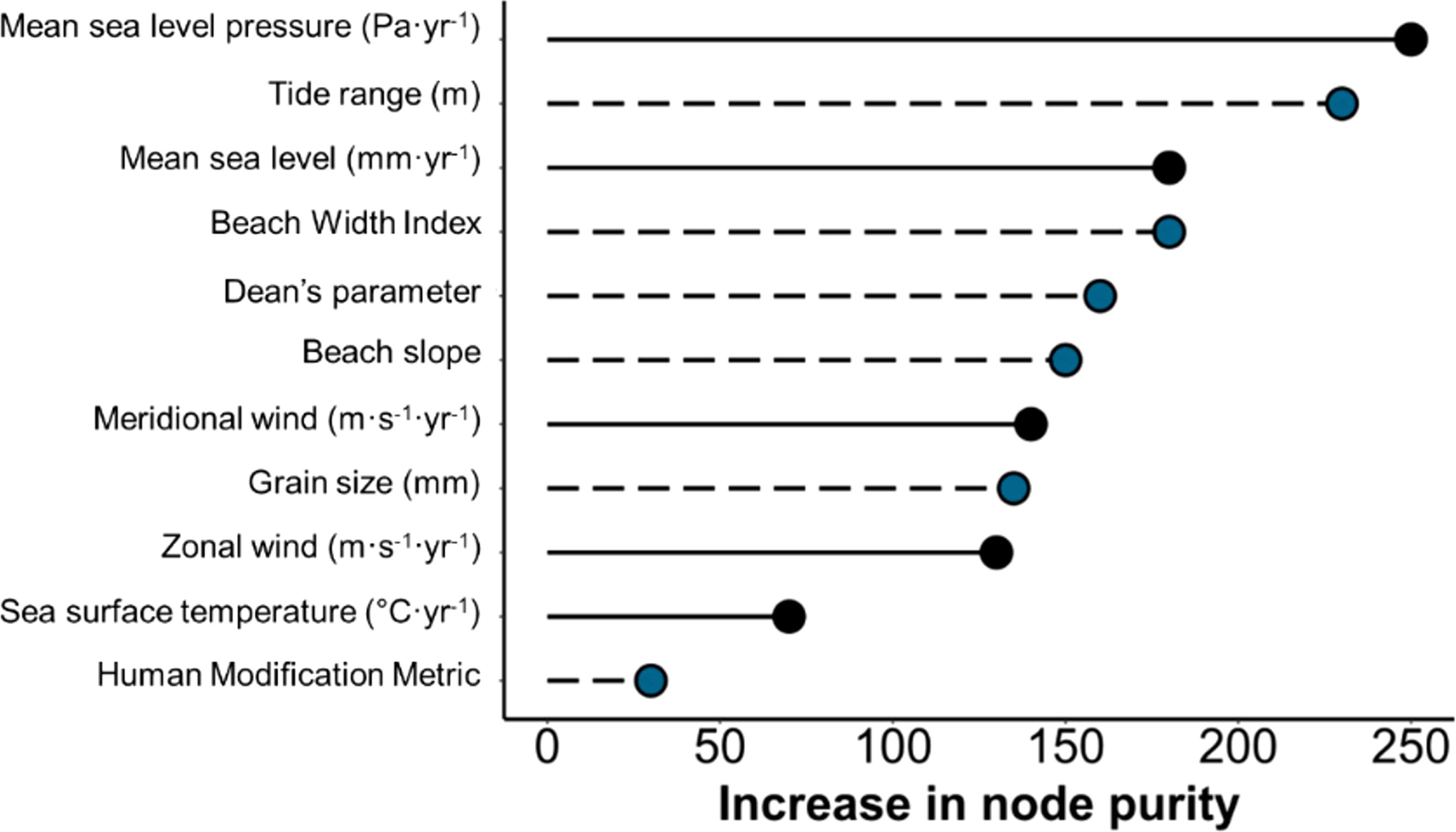
Figure 6 Variable importance plot resulting from the Random Forest analysis of the effects of local (dashed lines) and regional (solid lines) variables on beach erosion rates. The increase in node purity reflects the percent increase in the mean square error that would result from the removal of a given factor from the analysis (i.e., a measure of by how much including a variable increases model accuracy). Mean sea level, zonal and meridional winds, sea surface temperature and mean sea level pressure refer to anomaly trends (see text).
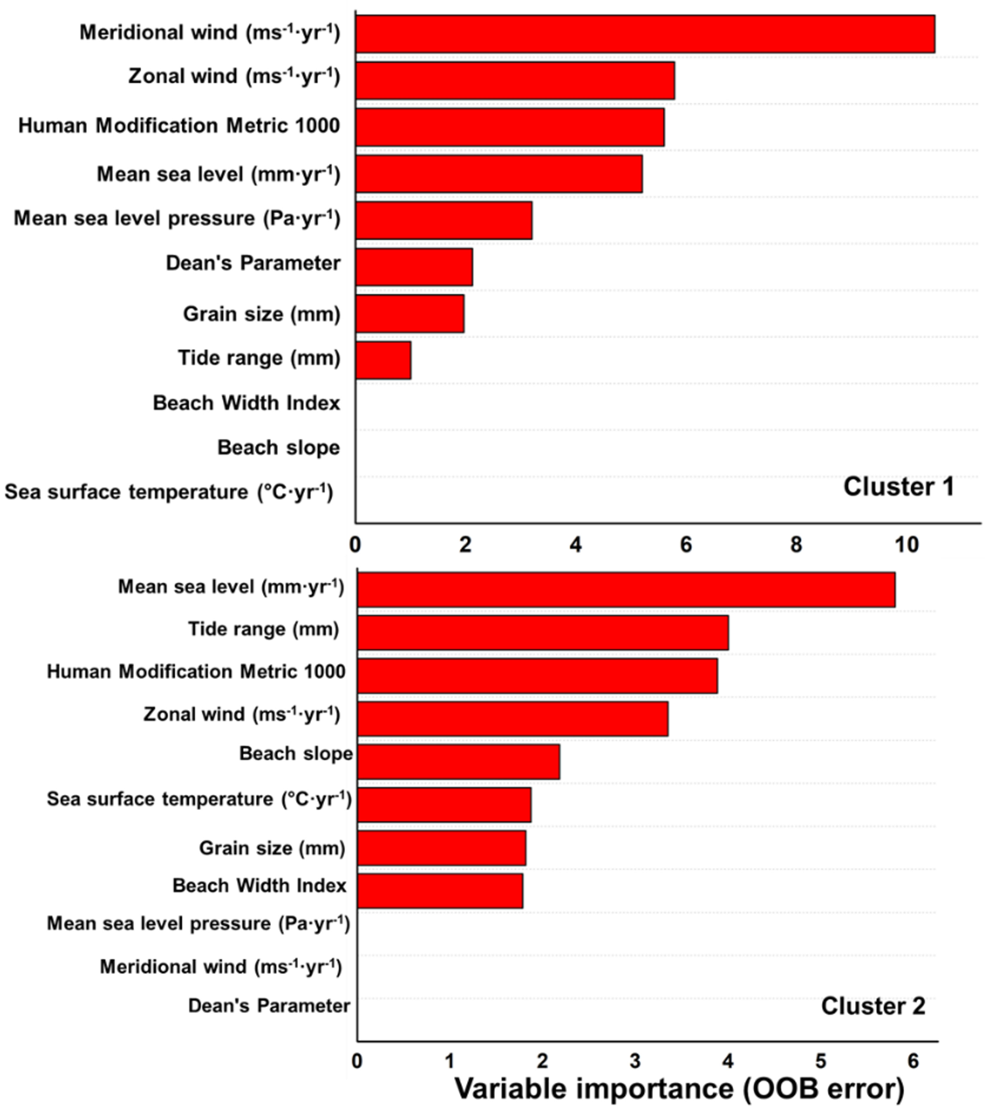
Figure 7 Variable importance plot resulting from a Random Forest analysis to assess the effects of local and regional variables on beach erosion rates in Clusters 1 and 2 (see Table 1 and Figure 5). The Out-Of-Bag error (OOB error) was used to assess the accuracy of single variables in describing erosion rates. OOB error evaluates the contribution of each variable to the estimation of the target variable by measuring how much the estimation worsens when excluding each variable, one at a time, from the set of predictors. Positive values of OOB error indicate that the variable is important, and the magnitude of importance is described by the absolute value of how much the target estimation worsens. Values equal to zero indicate no importance in the target estimation. Note the different X-axis scales. Mean sea level, zonal and meridional winds, sea surface temperature, and mean sea level pressure refer to anomaly trends (see text).
The PDPs revealed that erosion rate trends were positively associated with regional variables (Figure 8, left). Among them, mean sea level pressure and mean sea level exhibited a positive association with erosion rates across a range of beach conditions, from stable beaches to extreme erosional situations (Figure 8, left). On the other hand, the zonal and meridional winds were good predictors of erosion rates in beaches undergoing conditions of slight accretion to severe erosion. Sea surface temperature was also a good predictor from slight accretion to intense erosion (see also Figure S3).
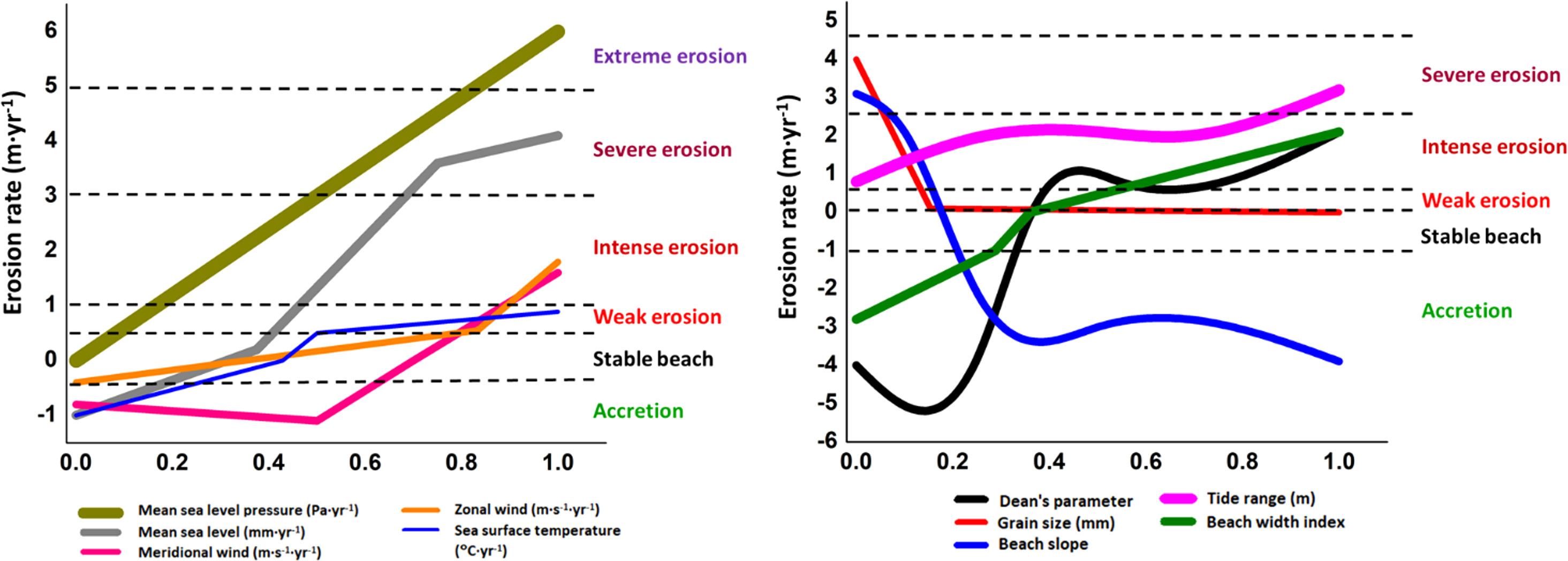
Figure 8 Partial dependence plots (PDPs) showing the relationships between erosion rates and local and regional predictor variables. PDPs place emphasis on those sections of the target variable’s domain where these relationships are strong. Line thickness is proportional to the importance of each variable assessed by Random Forest analyses (see Figure 6) and calculated separately for each response variable through Out-Of-Bag error estimation. Note the different Y-axis scales. Horizontal dashed lines indicate the limits of the erosion/accretion beach categories. The independent variables were scaled in a range from 0 to 1. As the independent variable is ‘erosion rate’, erosive states correspond to positive Y-axis values, whereas accretive states correspond to negative erosion rate values.
Local variables also demonstrated relevance as predictors of erosion rates (Figure 8, right, see also Figure S3). Grain size and beach slope exhibited inverse relationships with the target variable, indicating increasing erosion rates on beaches with gentle slopes and fine grain sizes. Grain size proved to be a good predictor from stable situations to severe erosion, whereas beach slope was more effective in predicting erosion rates from clear accretion to severe erosion (Figure 8, right). Tide range was positively associated with erosion rates, indicating increasing erosion from microtidal to macrotidal beaches, and being a good predictor across stable situations to intense erosion (Figure 8). Furthermore, compound beach indices, such as Dean’s parameter and Beach Width Index, exhibited a positive correlation with erosion rates, implying increasing erosion rates towards wide dissipative and ultradissipative beaches. Dean’s parameter was a reliable predictor across conditions ranging from accretion to intense erosion, while the Beach Width Index became relevant in predicting erosion rates from clear accretion to severe erosion. Overall, regional variables defined conditions conducive to increased erosion rates, while local variables shaped beach dynamics, either reinforcing the effect of regional variables or enhancing a beach’s resistance to erosion, sometimes counteracting at the local level the erosive trend triggered by regional factors.
The analysis allowed for the identification of beaches with varying rates of change. Out of the 315 sandy beaches in the database, 32% were found to be affected by erosion rates of various magnitudes, while 27% were in stable conditions, and 41% were experiencing accretion. When considering the four erosion categories and discriminating by cluster, there was an increase in the representation of beaches experiencing erosion from reflective to dissipative states (Figure S4). Specifically, among the 133 beaches grouped in Cluster 1 (microtidal reflective beaches), 26% experienced erosion. This trend continued with 33% of the 108 beaches in Cluster 2 (intermediate microtidal beaches) experiencing erosion, followed by 39% of the 51 beaches in Cluster 3 (intermediate mesotidal), and 43% of the 21 beaches in Cluster 4 (dissipative macrotidal). Cluster 5 (ultradissipative macrotidal) consisted of one beach in stable conditions and another beach experiencing intense erosion (50%) (Table 3). Globally, 66 (21%) sandy beaches contained in our dataset are facing intense, severe or extreme erosion rates (Table 3).
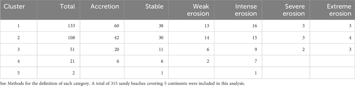
Table 3 Number of beaches facing accretion, stability and erosion, in the latter discriminated by a gradient of intensity from weak to extreme erosion.
Discussion
Our research provides groundbreaking insights into the combined impact of local and regional drivers on global sandy beach erosion, addressing a critical gap in multiscale understanding. Among the regional drivers, mean sea level pressure and mean sea level itself, along with several local drivers like tide range, beach slope and width, and Dean’s parameter, have emerged as the key determinants influencing long-term trends in coastal evolution processes. These results highlight the importance of considering the combined effects of multiple drivers in understanding the relative roles of local and regional processes in shaping long-term erosional trends. Our findings also carry management implications for these ecosystems, which are at risk in several regions of the world.
The assembly of a database containing unique in situ information on key physical variables from 315 sandy beaches covering the whole morphodynamic spectrum, combined with satellite information, enabled us to decipher the relative contribution of different variables driving coastal evolution at various spatial scales. Our database, spanning all continents and latitudes, could be considered representative of the global situation. Mixed methods, involving in situ data and satellite information, enhanced our ability to assess variations in coastline evolution with a perspective on fundamental beach habitat features. Satellite information provided a broad view of global patterns in specific variables operating at large spatial scales (e.g., sea level pressure, sea surface temperature, zonal and meridional winds), whereas in situ data extracted from published studies offered detailed information specific to individual sandy beaches (e.g., tide range, beach slope and width, grain size). Therefore, our study highlights the importance of site-based research that specifically addresses changes in essential physical variables in sandy beaches as a complementary source of validation for satellite derived information, which could be used to design and implement effective conservation and management strategies (Harris et al., 2011; Orlando et al., 2020; Orlando et al., 2021; Checon et al., 2022). A further step forward should be to assess long-term variations in the variables measured in situ (see e.g., Ortega et al., 2013).
The clustering process enabled the identification of 5 groups, ranging from wave-dominated to tide-modified systems. Local factors held the highest statistical relevance in demarcating the groups, emphasizing the outstanding role of essential beach variables (slope, grain size), their composite derivatives (beach width and Dean’s parameter) and tide range in the characterization of these clusters (Table 2). These trends reveal a progressive gradient of energy dissipation ranging from microtidal reflective to ultradissipative macrotidal beaches. The results from the clustering process further highlight the significance of tides in the dynamics of these narrow interfaces between land and sea, with tide range emerging as an important driver modulating coastal geomorphological processes (Table 2). The outstanding contribution of other local variables to the clustering process, including beach width and slope, grain size and Dean’s parameter, further emphasizes the importance of analyzing tide range along with wave conditions and other local factors. Tide range has also been identified as a pivotal correlate of faunal diversity patterns in sandy beaches (Defeo and McLachlan, 2013; Barboza and Defeo, 2015; Defeo et al., 2017). Thus, understanding its significance is of vital importance if we are to address emerging issues impacting the ecological, geomorphological, and hydrodynamic aspects of these ecosystems.
In accordance with the Bruun Rule (Bruun, 1962), our analysis of the role of local factors has clearly shown that the wider and flatter a beach, the greater the likely rate of erosion, hence greatest erosion on ultradissipative macrotidal beaches. On the matter of local conditions, McLachlan et al. (2018) developed a two-step model to determine the beach type and state, including a simple method to quantify wave conditions: the first step involves combining breaker height with tide range to identify whether waves or tides predominantly influence beach morphology, thereby defining beach types as wave-dominated, tide-modified, or tide-dominated; then, by incorporating breaker height, period, and sand particle size (the main determinants of Dean’s parameter included in this paper), the beach state can be easily characterized (McLachlan et al., 2018). Considering the findings presented in this paper, this approach to identifying beach type and state could also aid in developing practical management recommendations for sandy beach ecosystems and, indeed, the whole LAZ, when addressing not only changes in coastal evolution but also the differential effects of other pressures acting together (Costa et al., 2020; Defeo et al., 2021; Fanini et al., 2021; Costa et al., 2022).
The foregoing results had significant implications when examining trends in coastal evolution overall, particularly concerning the occurrence of differential erosion according to morphodynamic gradients. Erosion rates followed an increasing pattern from narrow and steep wave-dominated microtidal reflective beaches, through macrotidal intermediate and dissipative systems, to tide-modified ultradissipative beaches, following the grouping order defined in the clustering process. This finding is consistent with the theoretical framework developed for sandy beaches, which suggests an increasing erosional gradient from microtidal reflective conditions with accretionary characteristics to macrotidal ultradissipative beaches with erosional features (McLachlan et al., 2018). However, the morphodynamics of a beach are continually responding to changes in wave regime, meaning variations in state, erosion/accretion dynamics and the development of rhythmic alongshore features (Bacino et al., 2019; Jackson and Short, 2020; Castelle and Masselink, 2022). This dynamic perspective of ocean shores should be considered when assessing beach erosion rates.
The Random Forest analysis demonstrated the subtle combination of regional and local drivers influencing beach erosion rates. Indeed, mean sea level pressure was a relevant large-scale explanatory driver of worldwide trends, followed in decreasing order of importance by tide range, mean sea level, Beach Width Index, Dean’s parameter and beach slope (Figure 6). Mean sea level pressure can affect sandy beach erosion rates through its influence on wind patterns and wave generation. The intensification of high mean sea level pressure systems can create pressure gradients and stronger winds. Thus, the strength and direction of winds influenced by sea level pressure (Figure 1) can directly influence erosion rates (Kalma et al., 1988). Our findings align with recent research that suggests shifting pressure belts and wave climates may have comparable, if not greater, impacts on many beaches than sea level rise (Reboita et al., 2019; Short, 2022). This supports the notion that changes in atmospheric pressure patterns and wave conditions play a significant role in shaping beach erosion processes alongside the well-documented influence of rising sea levels (Dodet et al., 2019; Short, 2022). Orlando et al. (2019) also showed that long-term variations in beach area were negatively affected by an increase in sea level and climatic conditions, being positively correlated with sea surface temperature anomalies and offshore winds (which favored accretion) and negatively correlated with onshore winds and intense El Niño Southern Oscillation (ENSO) events (favoring erosion).
Tide range emerged as the second significant variable in explaining erosion rates in sandy beaches. It plays a crucial role in shaping coastal processes and influencing beach erosion dynamics, dependent on the coastal topography and bathymetry (Jackson et al., 2022). Tide range directly impacts erosion rates by affecting wave energy and sediment transport. Higher wave energy during high tides can lead to more pronounced beach erosion, dislodging and transporting sediment (Yuan et al., 2020). Notably, in macrotidal beaches, such erosive power of waves can be amplified, especially when combined with storm events or high-energy wave conditions. Dean’s parameter, a measure of the ability of waves to transport sand (Short, 1996; Jackson and Short, 2020), together with beach width, proved to be crucial, both in the clustering process and in explaining coastal evolution patterns, highlighting again the role of local variables as drivers of erosion trends. Nonetheless, the impact of tide range on erosion rates can differ depending on the local conditions (e.g., exposure, orientation), and its interplay with beach morphodynamic features and the wave climate is complex and deserves careful examination at the scale of individual beaches (Orlando et al., 2019; Gómez-Pujol and Orfila, 2020; Checon et al., 2022).
Mean sea level was identified as a significant regional variable influencing erosion rates. Higher sea levels intensify wave action, leading to sediment removal and beach reshaping. Consequently, beach erosion and sea level rise are interconnected processes (Bruun, 1988). With global sea levels rising due to climate change, sandy beaches face heightened risks of erosion. Coastal systems are increasingly sediment-starved, and this will likely interact with sea level rise to accelerate erosion (McLachlan and Defeo, 2018). Beaches located in low-lying and heavily developed coastal areas are especially vulnerable to sea level rise and erosion (Bindoff et al., 2019), which also highlights the importance of HMM as a potential explanatory variable for erosion trends, particularly in microtidal reflective and intermediate beaches (Clusters 1 and 2). Sandy beaches, however, exhibit diverse forms and settings, with variations in orientation and exposure to wave action, resulting in site-specific and temporally variable responses to sea level rise. Therefore, there is no single, uniform response of beaches to rising sea levels, and regional-scale lenses of observation can overlook such fine-scale nuances (Castelle et al., 2018; Orlando et al., 2019; Cooper et al., 2020; Ferreira et al., 2023). Further, because of the high spatial variability in crustal subsidence rates (Menard, 1983; Di Natale et al., 2008), wave climates and tidal regimes, it is the set of local conditions, rather than a single global mean sea-level trend, that determines each locality’s vulnerability (Cooper et al., 2020). Projections have shown that sea level rise will not be uniform across the globe (Mengel et al., 2016) and, by the end of the 21st century, sea level rise would lead to the erosion and loss of beaches in many regions. This will undoubtedly impact recreational and tourism opportunities, and affect local economies that rely on beach-related activities in these social-ecological coastal systems (Bindoff et al., 2019; Fanini et al., 2021).
The analysis of PDPs reinforced the results mentioned earlier and further underlines the significance of regional variables in influencing erosion rates across a diverse range of beach conditions (Figure 8). The positive associations identified between erosion rates and mean sea level pressure, mean sea level, zonal and meridional winds, and sea surface temperature emphasize the pivotal role these factors play in shaping erosion patterns (Pang et al., in press). Mean sea level pressure emerged again as a critical correlate, as evidenced by its highest relevance in relation to erosion rates across various conditions that ranged from stable beaches to extreme erosional situations (see Figure 8). Mean sea level also exhibits remarkable importance in its positive association with erosion rates, encompassing a broad spectrum of beach conditions ranging from accretionary states to severe erosion.
PDPs also showed that local variables played a significant role in predicting beach erosion rates at a broad range of beach conditions. However, the relative importance of these factors can vary widely depending on their morphodynamic characteristics (Ortega et al., 2013; Cooper et al., 2020; Short, 2022). The strong positive association between tide range and erosion rates clearly indicates that macrotidal beaches are more vulnerable to erosion than microtidal ones, as also depicted in several results portrayed in this paper. Tide range was particularly meaningful for beaches facing intense and severe erosion (Figure 8, see also Kirby, 2000). Moreover, the positive association between the compound indices (Dean’s parameter and Beach Width Index) and erosion rates implied that wider dissipative and ultradissipative beaches are more prone to erosive trends, both indices being reliable predictors across conditions ranging from accretionary states to beaches facing intense erosion. The well-known inverse relationship between grain size and beach slope, when considered together with erosion rates, reinforces the notion that beaches with fine grain sizes and gentle slopes (i.e., dissipative beaches) are more susceptible to erosion processes (Leadon, 2015). Beach slope was more effective in predicting erosion rates across accretionary to severely eroded situations, indicating its importance in understanding erosion dynamics in a wide range of beach conditions.
Overall, PDPs indicated that the combined influence of regional variables can contribute to high erosion rates, but the immediate effect is more closely related to local conditions. Thus, local variables have the potential to either amplify the effects of regional variables on erosion rates or bolster a beach’s resistance to erosion, thereby mitigating the erosive trends initiated by regional factors (Eichentopf et al., 2019). Beach resistance to erosion is primarily associated with specific combinations of beach width, beach slope and Dean’s parameter, with the latter two being the most useful indicators of this resistance. Low values of Dean’s parameter and high values of beach slope lead beaches toward stable and accretive states (Yates et al., 2009). The effects of these drivers on beach erosion depend on geographical location, local geology, and other local factors (Orlando et al., 2019). Indeed, the local geology plays a pivotal role in shaping beach morphology through its control of sediment size and availability; therefore, sandy beaches may experience distinct erosion patterns due to variations in the resistance of geological materials to the forces of waves, tides, and weathering (Gallop et al., 2020; Jackson and Short, 2020).
The analysis of PDPs deconstructed by cluster and categorized into different erosion rate levels showed that more than one-fifth of the analyzed beaches are experiencing intense, extreme, or severe erosion rates (see Table 3). Furthermore, when examining beach erosion patterns by morphodynamic type, the emerging pattern reinforces the role of local and regional processes in influencing sediment budget trends (Masselink and Russell, 2013). Our findings support the expectation that dissipative beaches, characterized by their erosional nature, are more susceptible to the impacts of sea level rise and tend to erode more significantly compared to reflective beaches, which are typically accretionary in nature (McLachlan and Defeo, 2018; McLachlan et al., 2018). Reflective beaches usually have a wide berm that acts as a sand reservoir and a buffer against erosion. In contrast, dissipative beaches lack this protective buffer, and the intertidal slope leads directly to the dunes, which can be reached by very high tides (McLachlan et al., 2018). Considering that ultradissipative beaches represent the erosional extreme and reflective beaches represent the accretionary extreme among morphodynamic states, it is expected that dissipative beaches would respond more strongly to sea level rise and erode further than reflective beaches.
The Random Forest analysis performed for Clusters 1 and 2 highlighted the significant role of the HMM as a local variable that explained erosion trends, which was not readily apparent when considering the either the overall dataset or in the other 3 clusters (Figure 7). These two clusters, which together encompassed 76% of all analyzed beaches, mainly grouped wave-dominated microtidal reflective or intermediate beaches. Human impacts, such as urbanization, coastal development, and armoring, can significantly amplify erosion rates in these beaches. Intense human modifications often disrupt natural sediment supply and transport processes, reducing the sediment available for beach replenishment. This depletion of sediment, especially critical for the dune component of the LAZ, can lead to a more immediate and pronounced reduction or loss of upper beach zones in reflective beaches affected by local urbanization. Beyond this explanation, future studies should emphasize the deconstruction of the HMM index in order to assess the relative importance of its components in explaining erosion patterns. Indeed, this index combines various components representing human activities, all equally weighted during calculation, even though they may have different effects on beach erosion. Therefore, HMM could be correlated with the dependent variable for one or several components, but not for its cumulative value. Nevertheless, it has been shown that, at the 1000 m scale, the HMM can be positively related to impacts on beaches, making it a reliable proxy for assessing the effects of local urbanization on sandy beaches (Barboza et al., 2021), the deconstruction of the HMM into its components (see e.g., Corte et al., 2022; Costa et al., 2022) could allow for a more refined and accurate assessment of their relative contributions to coastal evolution.
Random Forests also highlighted the influence of wind anomalies and mean sea level (Cluster 1) and mean sea level and tide range (Cluster 2) as correlates of erosive trends. Therefore, both HMM and rising sea levels have contributed significantly to explaining the effects of local and regional variables on beach erosion rates. These results reinforce the notion that a major long-term threat facing sandy beaches worldwide is “coastal squeeze”, where the landward boundary of the LAZ is constrained due to seaward encroachment by human development, while the seaward boundary migrates landwards in response to sea level rise, compounded with other climate-related stressors (Defeo et al., 2009; Defeo et al., 2021). Indeed, rising sea levels amplify effects of storm surges, which are also increasing in size and frequency due to warming (Bindoff et al., 2019), pushing the LAZ landward and augmenting erosion rates (Summers et al., 2018; Orlando et al., 2019). Further, pulse perturbations such as the El Niño–Southern Oscillation, when superimposed on sea level rise, tend to exacerbate erosion (Barnard et al., 2015). Most beaches cannot respond naturally to coastal squeeze, landward retreat being blocked by development (Haasnoot et al., 2021; Mach and Siders, 2021) and related coastal defence structures that limit the ability of beaches to migrate (Cooper et al., 2020). This is particularly the case in regions with high population density and coastal development, the consequence being loss of natural and human capital (Arkema et al., 2013; Bindoff et al., 2019). In contrast, areas without development have a low risk of beach loss, by allowing for unimpeded beach migration.
The effect of regional variables on sandy beach erosion patterns are clearly superimposed on the impact of climate change in explaining such trends. To be sure, our analysis has allowed us to identify hotspots where the combined effects of intensification of the anomalies in mean sea level pressure and increasing onshore winds (Figure 1), warming rates significantly higher than the global average (Figure 2), and rising sea levels (Figure 3) may be synergistically accelerating erosion rates. These hotspots include for example regions in the Southwestern Atlantic, the Indian Ocean, and Southeast Pacific, over a similar latitudinal range (Figures 1–3). Projections indicate that, by the end of this century, wind-driven subtropical boundary currents in both the northern and southern hemispheres will strengthen and shift towards the poles. This shift will bring higher temperatures and an increased risk of storms to temperate latitudes (Wu et al., 2012; Yang et al., 2016). The release of heat by warm currents will contribute to heat transfer from the tropics to the poles, potentially leading to increased storminess in temperate latitudes (Yang et al., 2020). These processes could result in coastal erosion, with rising sea levels exacerbating the situation, especially for sandy beaches located in southern temperate latitudes that are experiencing warming hotspots (Hobday and Pecl, 2014, see Figure 2). These areas are distinguished by a complex system of ocean currents, leading to the formation of oceanographic regimes and fronts with high primary production. These conditions sustain a rich sandy beach biodiversity and support the development of small-scale fisheries that hold critical socioeconomic value for vulnerable communities (Hobday et al., 2016; Franco et al., 2020; Gianelli et al., 2021). Consequently, these hotspot areas need effective management and conservation strategies in a climate change scenario, not only directed to safeguard biodiversity but also to support the livelihoods and well-being of coastal communities that depend on these resources. As sandy beach ecosystems face erosion and degradation, management and policy efforts are needed to foster their resilience in the face of ongoing climate changes and other human-induced pressures, such as increasing urbanization, industrialization, and resource use (Orlando et al., 2020; Defeo and Elliott, 2021).
Conclusion
Our analysis has shed light on the complex interactions between local and regional drivers in shaping beach erosion dynamics. Using a comprehensive database integrating unique in situ data with satellite information, we have shown that both local and regional drivers affect coastal evolution. Regional variables, which encompass the beach’s geographical context, defined the conditions conducive to increased erosion rates, whereas local variables, like grain size, beach slope, tide range, and wave energy (captured in beach indices), shaped beach dynamics. These findings highlight the need for approaches that address both local and regional drivers to understand and mitigate the processes and impacts of beach erosion. These results also provide valuable insights for beach managers regarding interactions between local and regional drivers, as well as the value of incorporating anthropogenic effects in decision-making using cumulative HMM values.
The issue of beach erosion is exacerbated by the simultaneous forces of rising sea levels and coastal development, acting together on the sandy littoral as coastal squeeze. This constriction has cascading effects over a far wider area than just the beach, spanning both the marine and terrestrial components of the coast. Further, we need to be cognizant of the critical challenge of the social–ecological traps and collapses that will follow in these ecosystems at risk (Defeo et al., 2021). These findings reinforce the notion that, to maintain their ecosystem functions while supporting recreational and aesthetic demands, sandy beaches, together with their associated foredunes and surf zones, must be considered holistically as tightly coupled social-ecological systems (McLachlan and Defeo, 2018; Harris and Defeo, 2022; McLachlan and Defeo, 2023). Understanding the interactions between local and regional variables and erosion rates is complex but necessary in order to deal with both short-term and long-term changes in these endangered ecosystems (Cooper et al., 2020). A multi-level approach is essential for sustaining effective management policies centered on a comprehensive understanding of the sandy littoral. This strategy should include implementing nature-based solutions tailored to local contexts and adaptable on a global scale, specifically aimed at mitigating coastal retreat (Pontee et al., 2016; Kumar et al., 2021).
Data availability statement
The in-situ information used in this article is not readily available, because the authors are working on several papers related to this dataset that took years to be built. We will make the dataset available once we finish a couple of pending papers. Requests to access this information should be directed to Omar Defeo (odefeo@dinara.gub.uy).
Author contributions
FB: Conceptualization, Data curation, Methodology, Writing – review & editing, Investigation, Formal Analysis, Software. LO: Conceptualization, Data curation, Investigation, Methodology, Writing – review & editing. LC: Conceptualization, Data curation, Investigation, Methodology, Writing – review & editing. LF: Data curation, Investigation, Writing – review & editing. CB: Data curation, Investigation, Writing – review & editing. AM: Investigation, Writing – review & editing. OD: Conceptualization, Data curation, Investigation, Methodology, Supervision, Writing – original draft, Writing – review & editing.
Funding
The author(s) declare financial support was received for the research, authorship, and/or publication of this article. LC was supported by Fundação de Amparo à Pesquisa do Estado do Rio de Janeiro (FAPERJ), grant number E-26.210.384/2022 and E-26.200.620/2022. CB was supported by FAPERJ (E-26/201.382/2021). OD was supported by Comisión Sectorial de Investigación Científica of Uruguay (CSIC Grupos ID 32).
Acknowledgments
FB thanks his friend Dr. Fabrizio Bazzocchi for the constructive discussions and continuous support.
Conflict of interest
The authors declare that the research was conducted in the absence of any commercial or financial relationships that could be construed as a potential conflict of interest.
Publisher’s note
All claims expressed in this article are solely those of the authors and do not necessarily represent those of their affiliated organizations, or those of the publisher, the editors and the reviewers. Any product that may be evaluated in this article, or claim that may be made by its manufacturer, is not guaranteed or endorsed by the publisher.
Supplementary material
The Supplementary Material for this article can be found online at: https://www.frontiersin.org/articles/10.3389/fmars.2023.1270490/full#supplementary-material
References
Almar R., Ranasinghe R., Bergsma E. W., Diaz H., Melet A., Papa F., et al. (2021). A global analysis of extreme coastal water levels with implications for potential coastal overtopping. Nat. Commun. 12, 3775. doi: 10.1038/s41467-021-24008-9
Arkema K. K., Guannel G., Verutes G., Wood S. A., Guerry A., Ruckelshaus M., et al. (2013). Coastal habitats shield people and property from sea-level rise and storms. Nat. Clim. Change 3, 913–918. doi: 10.1038/nclimate1944
Bacino G. L., Dragani W. C., Codignotto J. O. (2019). Changes in wave climate and its impact on the coastal erosion in Samborombón Bay, Río de la Plata estuary, Argentina. Estuar. Coast. Shelf Sci. 219, 71–80. doi: 10.1016/j.ecss.2019.01.011
Barboza F. R., Defeo O. (2015). Global diversity patterns in sandy beach macrofauna: a biogeographic analysis. Sci. Rep. 5, 14515. doi: 10.1038/srep14515
Barboza C. A., Mattos G., Soares-Gomes A., Zalmon I. R., Costa L. L. (2021). Low densities of the ghost crab Ocypode quadrata related to large scale human modification of sandy shores. Front. Mar. Sci. 8, 589542. doi: 10.3389/fmars.2021.589542
Barnard P. L., Short A. D., Harley M. D., Splinter K. D., Vitousek S., Turner I. L., et al. (2015). Coastal vulnerability across the Pacific dominated by El Nino/Southern oscillation. Nat. Geosci. 8, 801–807. doi: 10.1038/ngeo2539
Bendixen M., Best J., Hackney C., Iversen L. L. (2019). Time is running out for sand. Nature 571, 29–31. doi: 10.1038/d41586-019-02042-4
Bindoff N. L., Cheung W. W. L., Kairo J. G., Aristegui J., Guinder V. A., Hallberg R., et al. (2019). “Changing ocean, marine ecosystems, and dependent communities,” in IPCC Special Report on the Ocean and Cryosphere in a Changing Climate. Ed. Pörtner H.-O., et al (Geneva, Switzerland: IPCC), 477–587.
Bisht A. (2022). Sand futures: post-growth alternatives for mineral aggregate consumption and distribution in the global south. Ecol. Econ. 191, 107233. doi: 10.1016/j.ecolecon.2021.107233
Bland J. M., Altman D. G. (1996). Statistics notes: Transforming data. BMJ 312, 770. doi: 10.1136/bmj.312.7033.770
Blott S. J., Pye K. (2001). GRADISTAT: a grain size distribution and statistics package for the analysis of unconsolidated sediments. Earth Surf. Proc. Land. 26, 1237–1248. doi: 10.1002/esp.261
Brooks S. (2020). Disappearing beaches. Nat. Clim. Change 10, 188–190. doi: 10.1038/s41558-019-0656-9
Bruun P. (1962). Sea-level rise as a cause of shore erosion. J Waterways Harbors Division 88, 117–130. doi: 10.1061/JWHEAU.0000252
Bruun P. (1988). The Bruun rule of erosion by sea-level rise: a discussion on large-scale two-and three-dimensional usages. J. Coast. Res. 4, 627–648.
Castelle B., Guillot B., Marieu V., Chaumillon E., Hanquiez V., Bujan S., et al. (2018). Spatial and temporal patterns of shoreline change of a 280-km high-energy disrupted sandy coast from 1950 to 2014: SW France. Estuar. Coast. Shelf Sci. 200, 212–223. doi: 10.1016/j.ecss.2017.11.005
Castelle B., Masselink G. (2022). Morphodynamics of wave-dominated beaches. Cambridge Prisms: Coast. Futures 1, e1. doi: 10.1017/cft.2022.2
Cavalieri D., Parkinson C., Gloerson P., Zwally H. J. (1997). Sea ice concentrations from Nimbus-7 SMMR and DMSP SSM/I passive microwave data, June to September 2001 (Boulder, Colo: Natl. Snow and Ice Data Cent.). Available at: http://nsidc.org/data/nsidc-0051.html.
Checon H. H., Esmaeili Y. S., Corte G. N., Malinconico N., Turra A. (2022). Locally developed models improve the accuracy of remotely assessed metrics as a rapid tool to classify sandy beach morphodynamics. PeerJ 10, e13413. doi: 10.7717/peerj.13413
Cooper J. A. G., Masselink G., Coco G., Short A. D., Castelle B., Rogers K., et al. (2020). Sandy beaches can survive sea-level rise. Nat. Clim. Change 10, 993–995. doi: 10.1038/s41558-020-00934-2
Corte G. N., Checon H. H., Esmaeili Y. S., Defeo O., Turra A. (2022). Evaluation of the effects of urbanization and environmental features on sandy beach macrobenthos highlights the importance of submerged zones. Mar. pollut. Bull. 182, 113962. doi: 10.1016/j.marpolbul.2022.113962
Costa L. L., Fanini L., Zalmon I. R., Defeo O., McLachlan A. (2022). Cumulative stressors impact macrofauna differentially according to sandy beach type: a meta-analysis. J. Environ. Manage. 307, 114594. doi: 10.1016/j.jenvman.2022.114594
Costa L. L., Zalmon I. R., Fanini L., Defeo O. (2020). Macroinvertebrates as indicators of human disturbances on sandy beaches: A global review. Ecol. Indic. 118, 106764. doi: 10.1016/j.ecolind.2020.106764
Craney T. A., Surles J. G. (2002). Model-dependent variance inflation factor cutoff values. Qual. Eng. 14, 391–403. doi: 10.1081/QEN-120001878
Defeo O., Barboza C. A., Barboza F. R., Aeberhard W. H., Cabrini T. M., Cardoso R. S., et al. (2017). Aggregate patterns of macrofaunal diversity: an interocean comparison. Glob. Ecol. Biogeogr. 26, 823–834. doi: 10.1111/geb.12588
Defeo O., Elliott M. (2021). The ‘triple whammy’ of coasts under threat–why we should be worried! Mar. pollut. Bull. 163, 111832. doi: 10.1016/j.marpolbul.2020.111832
Defeo O., McLachlan A. (2013). Global patterns in sandy beach macrofauna: Species richness, abundance, biomass and body size. Geomorphology 199, 106–114. doi: 10.1016/j.geomorph.2013.04.013
Defeo O., McLachlan A., Armitage D., Elliott M., Pittman J. (2021). Sandy beach social–ecological systems at risk: regime shifts, collapses, and governance challenges. Front. Ecol. Environ. 19, 564–573. doi: 10.1002/fee.2406
Defeo O., McLachlan A., Schoeman D. S., Schlacher T. A., Dugan J., Jones A., et al. (2009). Threats to sandy beach ecosystems: a review. Estuar. Coast. Shelf Sci. 8, 1–12. doi: 10.1016/j.ecss.2008.09.022
Di Natale M., Eramo C., Vicinanza D. (2008). Experimental investigation on beach morphodynamics in the presence of subsidence. J. Coast. Res. 24, 222–231. doi: 10.2112/1551-5036(2008)24[222:EIOBMI]2.0.CO;2
Dodet G., Melet A., Ardhuin F., Bertin X., Idier D., Almar R. (2019). The contribution of wind-generated waves to coastal sea-level changes. Surv. Geophys. 40, 1563–1601. doi: 10.1007/s10712-019-09557-5
Dormann C. F., Elith J., Bacher S., Buchmann C., Carl G., Carré G., et al. (2012). Collinearity: a review of methods to deal with it and a simulation study evaluating their performance. Ecography 36, 27–46. doi: 10.1111/j.1600-0587.2012.07348.x
Eichentopf S., Karunarathna H., Alsina J. M. (2019). Morphodynamics of sandy beaches under the influence of storm sequences: Current research status and future needs. Water Sci. Engineer 12, 221–234. doi: 10.1016/j.wse.2019.09.007
Esteves L. S., Finkl C. W. (1998). The problem of critically eroded areas (CEA): An evaluation of Florida beaches. J. Coast. Res. 26, 11–18.
Fanini L., Defeo O., Elliott M. (2020). Advances in sandy beach research. Local and global perspectives. Estuar. Coast. Shelf Sci. 234, 106646. doi: 10.1016/j.ecss.2020.106646
Fanini L., Piscart C., Pranzini E., Kerbiriou C., Le Viol I., Pétillon J. (2021). The extended concept of littoral active zone considering soft sediment shores as social-ecological systems, and an application to Brittany (North-Western France). Estuar. Coast. Shelf Sci. 250, 107148. doi: 10.1016/j.ecss.2020.107148
Ferreira A. T. S., de Oliveira R. C., Ribeiro M. C. H., Grohmann C. H., Siegle E. (2023). Coastal dynamics analysis based on orbital remote sensing big data and multivariate statistical models. Coasts 3, 160–174. doi: 10.3390/coasts3030010
Franco B. C., Defeo O., Piola A. R., Barreiro M., Yang H., Ortega L., et al. (2020). Climate change impacts on the atmospheric circulation, ocean, and fisheries in the southwest South Atlantic Ocean: a review. Clim. Change 162, 2359–2377. doi: 10.1007/s10584-020-02783-6
Gallop S. L., Kennedy D. M., Loureiro C., Naylor L. A., Muñoz-Pérez J. J., Jackson D. W., et al. (2020). Geologically controlled sandy beaches: Their geomorphology, morphodynamics and classification. Sci. Total Environ. 731, 139123. doi: 10.1016/j.scitotenv.2020.139123
Gianelli I., Ortega L., Pittman J., Vasconcellos M., Defeo O. (2021). Harnessing scientific and local knowledge to face climate change in small-scale fisheries. Glob. Environ. Change 68, 102253. doi: 10.1016/j.gloenvcha.2021.102253
Gómez-Pujol L., Orfila A. (2020). “Reflective–dissipative continuum,” in Sandy Beach Morphodynamics. Eds. Jackson D. W. T., Short A. D. (Amsterdam: Elsevier), 421–437.
Grumbine R. W. (1996). Automated passive microwave sea ice concentration analysis at NCEP (USA: NCEP/NWS/NOAA, 5200 Auth Road, Camp Springs), 13.
Haasnoot M., Lawrence J., Magnan A. K. (2021). Pathways to coastal retreat. Science 372, 1287–1290. doi: 10.1126/science.abi6594
Harris L. R., Defeo O. (2022). Sandy shore ecosystem services, ecological infrastructure, and bundles: New insights and perspectives. Ecosyst. Serv. 57, 101477. doi: 10.1016/j.ecoser.2022.101477
Harris L., Nel R., Schoeman D. (2011). Mapping beach morphodynamics remotely: a novel application tested on South African shores. Estuar. Coast. Shelf Sci. 92, 78–89. doi: 10.1016/j.ecss.2010.12.013
Hartigan J. A., Wong M. A. (1979). Algorithm AS 136: A k-means clustering algorithm. J. R Stat. Soc C-App. 28, 100–108. doi: 10.2307/2346830
Hijmans R. J., Bivand R., Forner K., Ooms J., Pebesma E., Sumner M. D. (2022). Package ‘terra’. (Vienna, Austria: Maintainer).
Hobday A. J., Cochrane K., Downey-Breedt N., Howard J., Aswani S., Byfield V., et al. (2016). Planning adaptation to climate change in fast-warming marine regions with seafood dependent coastal communities. Rev. Fish Biol. Fisher 26, 249–264. doi: 10.1007/s11160-016-9419-0
Hobday A. J., Pecl G. T. (2014). Identification of global marine hotspots: sentinels for change and vanguards for adaptation action. Rev. Fish Biol. Fisher 24, 415–425. doi: 10.1007/s11160-013-9326-6
Hrdina J., Návrat A., Vašík P. (2019). Conic fitting in geometric algebra setting. Adv. Appl. Clifford Al 29, 1–13. doi: 10.1007/s00006-019-0989-5
Jackson D. W., Short A. D., Loureiro C., Cooper J. A. G. (2022). Beach morphodynamic classification using high-resolution nearshore bathymetry and process-based wave modelling. Estuar. Coast. Shelf Sci. 268, 107812. doi: 10.1016/j.ecss.2022.107812
Kalma J. D., Speight J. G., Wasson R. J. (1988). Potential wind erosion in Australia: A continental perspective. J. Climatol. 8, 411–428. doi: 10.1002/joc.3370080408
Kalnay E., Kanamitsu M., Kistler R., Collins W., Deaven D., Gandin L., et al. (1996). The NCEP/NCAR 40-year reanalysis project. Bull. Amer. Meteorol. Soc 77, 437–472. doi: 10.1175/1520-0477(1996)077<0437:TNYRP>2.0.CO;2
Kannan K. S., Manoj K. (2015). Outlier detection in multivariate data. Appl. Math. Sci. 47, 2317–2324. doi: 10.12988/ams.2015.53213
Kennedy C. M., Oakleaf J. R., Theobald D. M., Baruch-Mordo S., Kiesecker J. (2019). Managing the middle: A shift in conservation priorities based on the global human modification gradient. Glob. Change Biol. 25, 811–826. doi: 10.1111/gcb.14549
Kirby R. (2000). Practical implications of tidal flat shape. Cont. Shelf. Res. 20, 1061–1077. doi: 10.1016/S0278-4343(00)00012-1
Kumar P., Debele S. E., Sahani J., Rawat N., Marti-Cardona B., Alfieri S. M., et al. (2021). Nature-based solutions efficiency evaluation against natural hazards: Modelling methods, advantages and limitations. Sci. Total Environ. 784, 147058. doi: 10.1016/j.scitotenv.2021.147058
Leadon M. (2015). Beach slope and sediment-grain-size trends as a basis for input parameters for the SBEACH erosion model. J. Coast. Res. 31, 1375–1388. doi: 10.2112/JCOASTRES-D-14-00134.1
Likas A., Vlassis N., Verbeek J. J. (2003). The global k-means clustering algorithm. Pattern Recogn. 36, 451–461. doi: 10.1016/S0031-3203(02)00060-2
Luijendijk A., Hagenaars G., Ranasinghe R., Baart F., Donchyts G., Aarninkhof S. (2018). The state of the world’s beaches. Sci. Rep. 8, 6641. doi: 10.1038/s41598-018-24630-6
Mach K. J., Siders A. R. (2021). Reframing strategic, managed retreat for transformative climate adaptation. Science 372, 1294–1299. doi: 10.1126/science.abh1894
Masselink G., Russell P. (2013). Impacts of climate change on coastal erosion. MCCIP Sci. Rev. 2013, 71–86. doi: 10.14465/2013.arc09.071-086
May D. A., Parmeter M. M., Olszewski D. S., McKenzie B. D. (1998). Operational processing of satellite sea surface temperature retrievals at the Naval Oceanographic Office. Bull. Amer. Met. Soc 79, 397–407. doi: 10.1175/1520-0477(1998)079<0397:OPOSSS>2.0.CO;2
McLachlan A., Defeo O. (2018). The Ecology of Sandy Shores. 3rd Edition (Amsterdam: Elsevier, Academic Press).
McLachlan A., Defeo O. (2023). Where will the children play? A personal perspective on sandy beaches. Estuar. Coast. Shelf Sci. 280, 108186. doi: 10.1016/j.ecss.2022.108186
McLachlan A., Defeo O., Short A. D. (2018). Characterising sandy beaches into major types and states: Implications for ecologists and managers. Estuar. Coast. Shelf Sci. 215, 152–160. doi: 10.1016/j.ecss.2018.09.027
Menard H. W. (1983). Insular erosion, isostasy, and subsidence. Science 220, 913–918. doi: 10.1126/science.220.4600.913
Mengel M., Levermann A., Frieler K., Robinson A., Marzeion B., Winkelmann R. (2016). Future sea level rise constrained by observations and long-term commitment. Proc. Natl. Acad. Sci. 113, 2597–2602. doi: 10.1073/pnas.1500515113
Mentaschi L., Vousdoukas M. I., Pekel J.-F., Voukouvalas E., Feyen L. (2018a). Global long-term observations of coastal erosion and accretion. Sci. Rep. 8, 12876. doi: 10.1038/s41598-018-30904-w
Mentaschi L., Vousdoukas M., Pekel J.-F., Voukouvalas E., Feyen L. (2018b). Global long-term shoreline evolution (European Commission, Joint Research Centre (JRC). Available at: http://data.europa.eu/89h/944f6d9b-2fbf-422e-ae3e-4b3aa391ed48. doi: 10.2905/944f6d9b-2fbf-422e-ae3e-4b3aa391ed48
Oksanen J. (2011) Multivariate analysis of ecological communities in R: vegan tutorial v. 2.02. Available at: http://cc.oulu.fi/~jarioksa/opetus/metodi/vegantutor.pdf.
Orlando L., Ortega L., Defeo O. (2019). Multi-decadal variability in sandy beach area and the role of climate forcing. Estuar. Coast. Shelf. Sci. 218, 198–203. doi: 10.1016/j.ecss.2018.12.015
Orlando L., Ortega L., Defeo O. (2020). Urbanization effects on sandy beach macrofauna along an estuarine gradient. Ecol. Indic. 111, 106036. doi: 10.1016/j.ecolind.2019.106036
Orlando L., Ortega L., Defeo O. (2021). Perspectives for sandy beach management in the Anthropocene: satellite information, tourism seasonality, and expert recommendations. Estuar. Coast. Shelf. Sci. 262, 107597. doi: 10.1016/j.ecss.2021.107597
Ortega L., Celentano E., Finkl C., Defeo O. (2013). Effects of climate variability on the morphodynamics of Uruguayan sandy beaches. J. Coast. Res. 29, 747–755. doi: 10.2112/JCOASTRES-D-13-00003.1
Pang T., Wang X., Nawaz R. A., Keefe G., Adekanmbi T. (in press). Coastal erosion and climate change: A review on coastal-change process and modeling. Ambio. doi: 10.1007/s13280-023-01901-9
Parr T., Wilson J. D. (2021). Partial dependence through stratification. MLWA 6, 100146. doi: 10.1016/j.mlwa.2021.100146
Pekel J.-F., Cottam A., Gorelick N., Belward A. S. (2016). High-resolution mapping of global surface water and its long-term changes. Nature 540, 418–422. doi: 10.1038/nature20584
Pontee N., Narayan S., Beck M. W., Hosking A. H. (2016). Nature-based solutions: lessons from around the world. Marit. Eng. 169, 29–36. doi: 10.1680/jmaen.15.00027
Prasad N. R., Patel N. R., Danodia A. (2021). Crop yield prediction in cotton for regional level using random forest approach. Spat. Inf. Res. 29, 195–206. doi: 10.1007/s41324-020-00346-6
Ramosaj B., Pauly M. (2019). Consistent estimation of residual variance with random forest Out-Of-Bag errors. Stat. Probab. Lett. 151, 49–57. doi: 10.1016/j.spl.2019.03.017
Reboita M. S., Ambrizzi T., Silva B. A., Pinheiro R. F., da Rocha R. P. (2019). The South Atlantic subtropical anticyclone: present and future climate. Front. Earth Sci. 7, 8. doi: 10.3389/feart.2019.00008
Reynolds R. W., Smith T. M., Liu C., Chelton D. B., Casey K. S., Schlax M. G. (2007). Daily high-resolution-blended analyses for sea surface temperature. J. Clim. 20, 5473–5496. doi: 10.1175/2007JCLI1824.1
Rodil I. F., Harris L. R., Lucrezi S., Cerrano C. (2022). “Sandy beach management and conservation: the integration of economic, social and ecological values,” in Sandy Beaches as Threatened Ecosystems: Environmental Problems and Possible Assessment and Management Solutions. Eds. Gonçalves S. C., Ferreira S. M. F. (Boca Raton: CRC Press), 251–294.
Rousseeuw P. J. (1987). Silhouettes: a graphical aid to the interpretation and validation of cluster analysis. Comput. Appl. Math. 20, 53–65. doi: 10.1016/0377-0427(87)90125-7
Short A. D. (1996). The role of wave height, period, slope, tide range and embaymentization in beach classifications: a review. Rev. Chil. Hist. Nat. 69, 589–604.
Short A. D. (2022). Australian beach systems: Are they at risk to climate change? Ocean Coast. Manage. 224, 106180. doi: 10.1016/j.ocecoaman.2022.106180
Summers A., Fletcher C. H., Spirandelli D., McDonald K., Over J.-S., Anderson T., et al. (2018). Failure to protect beaches under slowly rising sea level. Clim. Change 151, 427–443. doi: 10.1007/s10584-018-2327-7
Syakur M. A., Khotimah B. K., Rochman E. M. S., Satoto B. D. (2018). Integration k-means clustering method and elbow method for identification of the best customer profile cluster. IOP Conf. Ser.: Mater. Sci. Eng. 336, 012017. doi: 10.1088/1757-899X/336/1/012017
Torres A., Simoni M. U., Keiding J. K., Müller D. B., zu Ermgassen S. O., Liu J., et al. (2021). Sustainability of the global sand system in the Anthropocene. One Earth 4, 639–650. doi: 10.1016/j.oneear.2021.04.011
Turiano M. C., Cruz E. C. (2017). Simulative analysis of storm tide levels in Batanes Islands during September 2016. Typhoon Meranti Using the Coupled Delft3D-SWAN Numerical Models (ASIAN and PACIFIC COASTS 2017), 200–211. doi: 10.1142/9789813233812_0019
UNEP (2019). Sand and sustainability: Finding new solutions for environmental governance of global sand resources (Geneva, Switzerland: GRID-Geneva, United Nations Environment Programme).
UNEP (2022). Sand and sustainability: 10 strategic recommendations to avert a crisis (Geneva, Switzerland: GRID-Geneva, United Nations Environment Programme).
Vousdoukas M. I., Ranasinghe R., Mentaschi L., Plomaritis T. A., Athanasiou P., Luijendijk A., et al. (2020). Sandy coastlines under threat of erosion. Nat. Clim. Change 10, 260–263. doi: 10.1038/s41558-020-0697-0
Woodruff J. D., Irish J. L., Camargo S. J. (2013). Coastal flooding by tropical cyclones and sea-level rise. Nature 504, 44–52. doi: 10.1038/nature12855
Wu L., Cai W., Zhang L., Nakamura H., Timmermann A., Joyce T., et al. (2012). Enhanced warming over the global subtropical western boundary currents. Nat. Clim. Change 2, 161–166. doi: 10.1038/nclimate1353
Yang H., Lohmann G., Krebs-Kanzow U., Ionita M., Shi X., Sidorenko D., et al. (2020). Poleward shift of the major ocean gyres detected in a warming climate. Geophys. Res. Letter, 45, e2019GL085868. doi: 10.1029/2019GL085868
Yang H., Lohmann G., Wei W., Dima M., Ionita M., Liu J. (2016). Intensification and poleward shift of subtropical western boundary currents in a warming climate. J. Geophys. Res. Oceans 121, 4928–4945. doi: 10.1002/2015JC011513
Yates M. L., Guza R. T., O’reilly W. C. (2009). Equilibrium shoreline response: Observations and modeling. J. Geophys. Res. Oceans 114, C09014. doi: 10.1029/2009JC005359
Yuan R., Kennedy D. M., Stephenson W. J., Finlayson B. L. (2020). The multidecadal spatial pattern of erosion on sandstone shore platforms in south-eastern Australia. Geomorphology 371, 107437. doi: 10.1016/j.geomorph.2020.107437
Zhang Z. (1997). Parameter estimation techniques: A tutorial with application to conic fitting. Image Vis. Comput. 15, 59–76. doi: 10.1016/S0262-8856(96)01112-2
Keywords: sandy beaches, erosion, coastal evolution, urbanization, morphodynamics, climate change, satellite information, coastal squeeze
Citation: Bozzeda F, Ortega L, Costa LL, Fanini L, Barboza CAM, McLachlan A and Defeo O (2023) Global patterns in sandy beach erosion: unraveling the roles of anthropogenic, climatic and morphodynamic factors. Front. Mar. Sci. 10:1270490. doi: 10.3389/fmars.2023.1270490
Received: 31 July 2023; Accepted: 21 September 2023;
Published: 09 October 2023.
Edited by:
Elisabeth Marijke Anne Strain, University of Tasmania, AustraliaReviewed by:
Helena Granja, University of Minho, PortugalBarbara Zanuttigh, University of Bologna, Italy
Copyright © 2023 Bozzeda, Ortega, Costa, Fanini, Barboza, McLachlan and Defeo. This is an open-access article distributed under the terms of the Creative Commons Attribution License (CC BY). The use, distribution or reproduction in other forums is permitted, provided the original author(s) and the copyright owner(s) are credited and that the original publication in this journal is cited, in accordance with accepted academic practice. No use, distribution or reproduction is permitted which does not comply with these terms.
*Correspondence: Omar Defeo, b2RlZmVvQGRpbmFyYS5ndWIudXk=; b21hci5kZWZlb0BnbWFpbC5jb20=
†These authors have contributed equally to this work and share first authorship