Study of the origin and correction of compass measurement errors in Doppler current meters

Surface and subsurface currents are two of the Essential Climate Variables (ECVs) defined by the Global Climate Observing System (GCOS). In situ current measurements can be made by Eulerian methods with instruments on moorings fixed in space. These methods require the determination of two metrological quantities: the speed and the direction of the motion. Their measurement and calibration require the determination of reference velocities and the measure of the angular movement of seawater in relation to the measuring device, as well as of the measuring device in relation to a reference direction given by the magnetic North. This reference direction is determined by electronic compasses integrated into current meters and current profilers. Compasses are sensitive to their magnetic environment, and, therefore, to the objects and instruments that surround them. This publication describes experiments conducted with current meters and current profilers to measure the influence of different devices on the accuracy of their compass measurements. It gives some explanations about the origin of measurement errors and proposes solutions to correct or attenuate the defaults in direction measurements and the measured deviations. Correction formulas are given that can be applied to measured data. They allow the reduction of errors of several tens of degrees for data to be within the instrument’s specifications.

1 Introduction

Surface and subsurface currents are two of the Essential Climate Variables (ECVs) defined by the Global Climate Observing System or GCOS (https://gcos.wmo.int/en/essential-climate-variables). According to GCOS, observations of subsurface ocean velocity contribute to estimates of ocean transports of mass, heat, freshwater, and other properties from local to regional and basin to global scales. They are essential in resolving the wind and buoyancy-driven ocean circulation and the complex vertical velocity structure.

However, measuring current is also essential to build current charts useful for navigation and 3D models of oceanic circulation or more recently to improve the efficiency of submarine tidal turbines. In situ measurements can be made by Eulerian methods where instruments are installed on fixed moorings or Lagrangian methods where instruments are surface or subsurface buoys ‘anchored’ in a water mass, the trajectory of which can be followed by satellites. Marine currents studies can also be carried out on multiple spatial scales (from thousands of kilometers to less than one meter) and multiple temporal scales (from seconds to several decades).

This publication concentrates on Eulerian methods, particularly on current meters and current profilers used on mooring lines or mooring cages. Eulerian methods require the determination of two metrological quantities: the speed and the direction of the motion. From a metrological point of view, their measurement and calibration require the determination of reference velocities and the measurement of the angular movement of seawater in relation to the measuring device, as well as of the measuring device in relation to a reference direction given by the magnetic North. Most Eulerian acoustic instruments are based on the Doppler effect and direction measurements. In most of the applications, they replaced the rotor current meter technology. They can be standalone or vessel-mounted and they can be single-point or profiling. As described below, techniques have already been proposed for calibrating these instruments in terms of velocity, but none of them can determine the amplitude of the angular errors caused by the compasses they are fitted with. Here, we propose solutions for reducing the measurement errors induced by the magnetic environment of compasses.

The calibration of rotor current meters was performed in open tanks (International Organization for Standardization, 2007) or hydrodynamic channels (Camnasio and Orsi, 2011), though generally to maximum velocities included in the range 1–3 m/s. The calibration in direction was not included and the devices surrounding the facility could generate compass measurement errors. For Doppler current meters, the low particle concentration in these facilities is a problem. The low backscattering decreases the amplitude of the returned signal. That increases the detection noise and reduces the velocity range that can be explored. Additionally, taking into account the profiling range of profilers used in oceanography (from 1 m to several hundred of metres according to the acoustic wavelength of the instrument), this method can hardly be applied. It is possible to carry out inter-comparisons at sea as carried out in 2012 (Drozdowsky and Greenan, 2013) or in rivers (Boldt and Oberg, 2015), but these inter-comparisons are expensive, difficult to organize, and they allow only one part of the velocity range of instruments to be tested. If compass errors can be detected and if differences in speed as small as 1 cm/s can be measured as was the case in 2012, they remain differential measurements and they can hardly be corrected with accuracy. For rivers again, another author proposed in 2018 (Huang, 2018) a theoretical and semiempirical model calibrated on transect datasets to estimate the uncertainty of streamflow measurements made by an acoustic Doppler current profiler (ADCP) mounted on a moving platform. This method could be applied to oceanography using vessel-mounted ADCPs although it is not adapted to standalone Teledyne RD Instruments ADCPs or equivalent instruments of Nortek group called AQPs for ‘AQuadopp Profilers’. Considering the inconvenience of these methods, a technique was proposed in 2020 to validate the Doppler effect measurement. It is based on a calibration bench (Le Menn and Morvan, 2020) that allows the detection of anomalies in the measurement of the Doppler shifts made by the transducers of current meters and current profilers.

Standalone instruments can be single-points or profilers. They are mounted on mooring cages deployed on the seabed or they are mounted on mooring lines. For instruments fitted on mooring cables, a method was proposed to quantify the influence of mooring line motion on current measurements (Langlois and Maze, 1990) but nothing was proposed to correct the effect of accessories on the compass measurements. The inclination must be corrected, and for this purpose, current meters were equipped with tilt sensors. The direction of current is retrieved by the three slanted beams and a matrix calculation that used measured tilt angles. The direction of the instrument in relation to magnetic North is retrieved with a magnetic compass and the direction in relation to the true North is retrieved by applying a correction of magnetic declination.

Compasses are composed of triaxial magnetic sensors that measure the amplitude of the magnetic flux in the three space directions. Knowing the tilt angles, a matrix system is used to find the horizontal component of the terrestrial magnetic field. The direction of field lines can be perturbed by the magnetic environment, and thereafter, the measurements made by compasses can be altered by objects and instruments that surround them.

In this publication, we describe experiments made on current meters and current profilers to measure the influence of different devices on the accuracy of their compass measurements in an area where the horizontal component of the magnetic field is large (≈ 22,000 nT) and well-determined. Studies about the origin and the amplitude of these errors are rare, so that correction methods (applied to boats compasses) exist for many years (see section 6).

In order to be able to calibrate current meters in large numbers, either on their own or installed in mooring cages, a calibration platform was built based on a method published in 2007 (Le Menn and Le Goff, 2007). The platform itself was the subject of a second publication in 2014 (Le Menn et al., 2014), and the essence of this publication is summarized in section 2 with an updated uncertainty budget.

Batteries are known to generate magnetic disturbances and are the elements that most often affect compass accuracy. Few studies have been devoted to this problem. Section 3 is devoted to the study of these errors, with explanations on the origin of battery magnetism and measurements taken to test their influence. Oceanographers often wonder about the effect of metal elements that are in the vicinity of current meters on compass accuracy. Therefore, section 4 describes measurements taken on different current profilers in different mooring configurations with different current accessories.

Current profilers are often deployed with a CTD profiler fixed on a rosette of sampling bottles in a configuration called LADCP (Lowered Acoustic Doppler Current Profiler). For towed profilers, a 1995 publication shows a method to correct compass bias induced by ship vicinity (Munchow et al., 1995). This publication complements the work we are presenting in section 5, which is devoted to the study of the accessory’s effects of this particular configuration, which enables ocean profiles to be nearly fully characterized.

In summary, this paper describes experiments made on current meters and current profilers to measure the influence of different devices on the accuracy of compass measurements. Our work uses physical measurements and expands on previous works that relies on theoretical mathematical calculations (Denne, 1998; Doerfler, 2009) or were specific to issues associated with boat compasses (NGIA, 2004) or ADCP used on a mooring containing iron (von Appen, 2015). Others have attempted direct measurement of compass errors in current meters (e.g., Rezaali et al., 2016), but this method is very specific to the type of mooring employed. Here, we present empirical data collected in a controlled setting that should be applicable to a variety of current meter deployments. We propose explanations about the origin of measurement errors and solutions to correct or attenuate the measured deviations.

2 Description of equipment used and the method for compass and tilt sensors’ calibration

Two kinds of current meters have been used to test the effect of different accessories: a single point of the manufacturer Nortek Group called Aquadopp or AQD DW (Deep Water) and a profiler of the manufacturer Teledyne RDInstruments called Workhorse ADCP 300 kHz. The AQD DW is commonly used on mooring lines as described in Lefevre et al. (2019). This publication presents two of the nodes of the European Multidisciplinary Seafloor and water-column Observatory (EMSO) where temperature salinity and currents are monitored. The Workhorse ADCP is also used commonly on mooring lines as described in de Mendoza et al. (2022). This publication presents an 8-year-long dataset of monitoring activities conducted on the western margin of the Southern Adriatic Sea where two moorings have been placed since 2012 in sites that are representative of different morpho-dynamic conditions of the continental slope. The accessories used on these moorings have been tested and they are listed in Table 2. To be autonomous, AQDs are equipped with battery packs that can be alkaline or lithium technologies. ADCPs are also equipped with battery packs that can be internal or external in a container linked to the ADCP.

Current meters and accessories were fixed on a non-magnetic cage. This cage called Tripode is composed of three uprights and three horizontal aluminium posts on which three non-magnetic ballasts are placed (see Figures 1–4). Its horizontality is adjusted with a nut-and-bolt system. For each experiment, the mark of the current meter is aligned on the mark made in the middle of one arm of the cage, and this mark is aligned on the central axis of a non-magnetic platform that points in the 70° direction. This platform, which is approximately 2.5 m in diameter, can be rotated and tilted. It is described in Le Menn et al. (2014). It is placed on land where the magnetic field is mapped (on a 20 x 20 m plot).

Figure 1

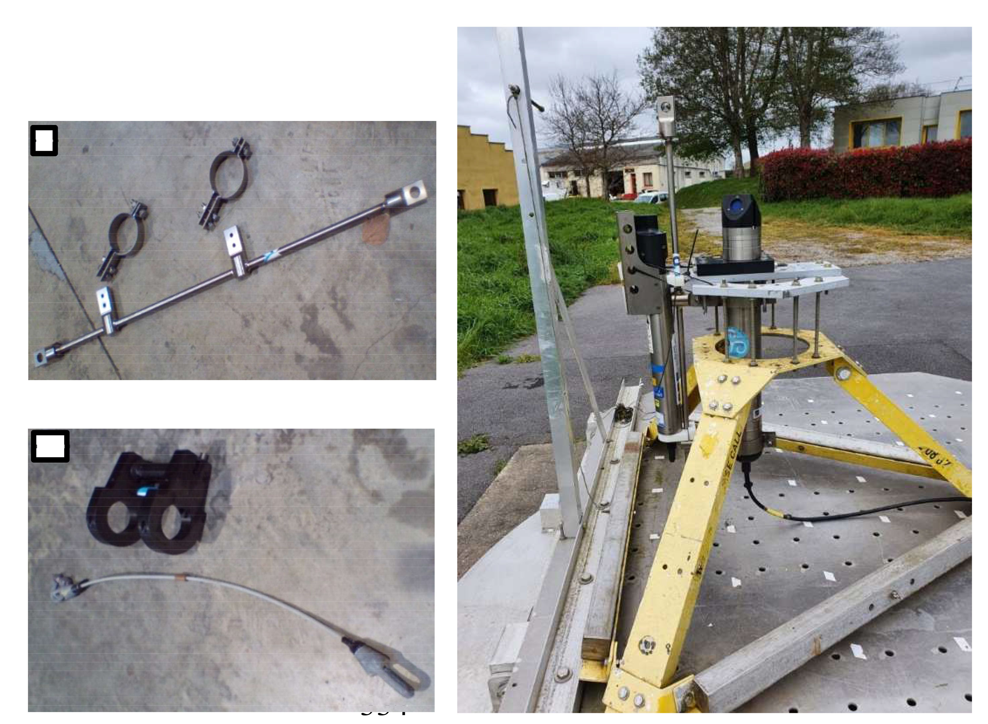
Figure 1 The first photo on the left is the shaft and the ‘clamps’ used to fix the CTD SBE 37 Microcat. The second photo on the left is the other clamps and inox cable used on mooring lines. The photo on the right is the titanium shaft and CTD SBE 37 MicroCAT fixed close to the AQD in a mooring configuration.

Figure 2

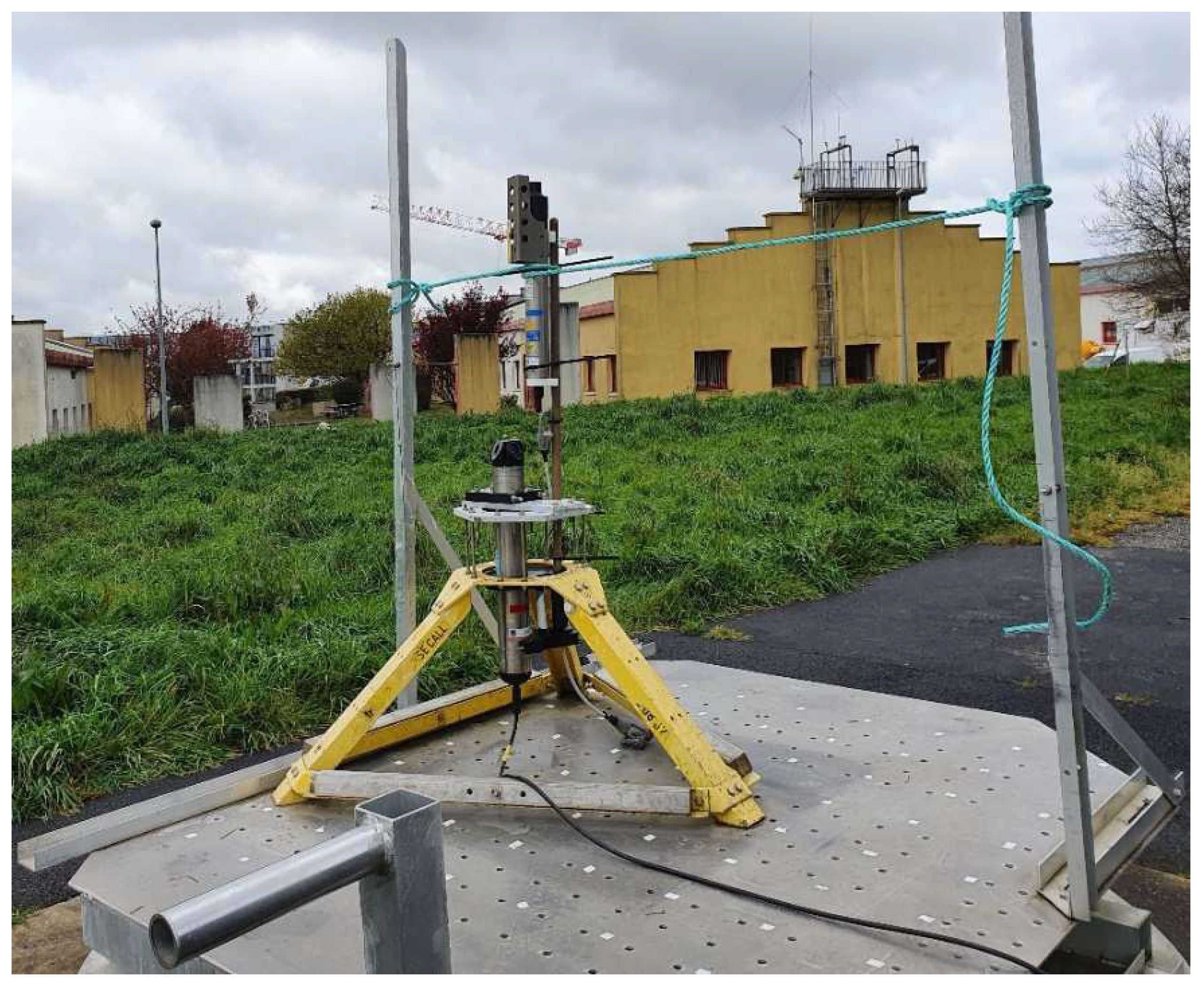
Figure 2 Third tested configuration. The SBE 37 is mounted on a mooring cable and the AQD is fixed to the cable with a clamp.

Figure 3

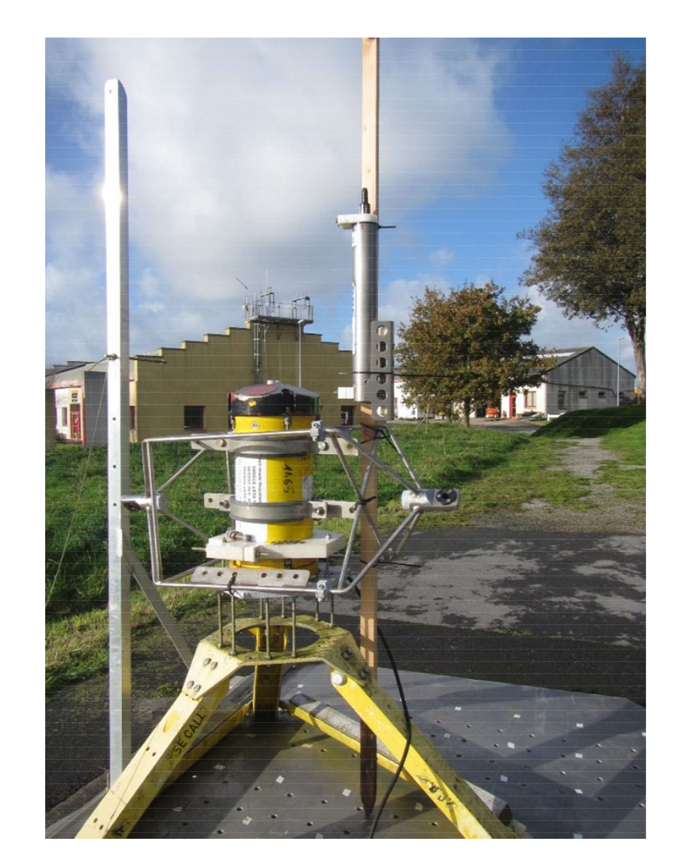
Figure 3 Metallic frame placed on the ADCP equipped with the two collars, and SBE 37 placed higher than the ADCP.

Figure 4

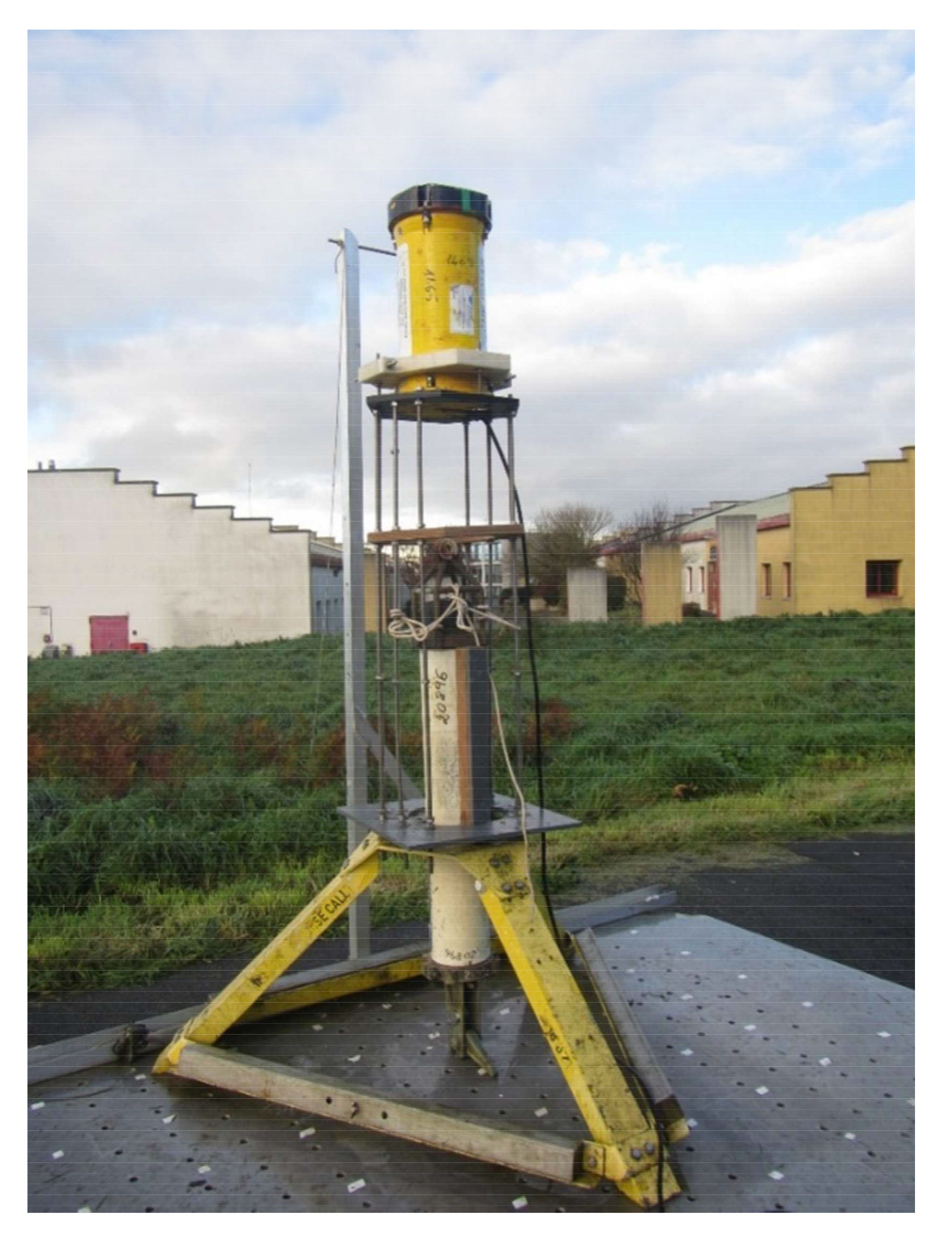
Figure 4 Test of the effect of the acoustic releaser placed 86 cm under the ADCP.

The platform is located in an area where the magnetic gradients are the weakest, i.e., where there are no magnetic anomalies that could locally perturb the direction of field lines. Figure 5 shows the results of the magnetic cartography with the magnetic anomalies obtained after the correction of the external temporal variations and of the secular variation of the terrestrial field. These corrections are calculated by subtracting the International Geomagnetic Reference Field (IGRF global model, Alken et al., 2021).

Figure 5

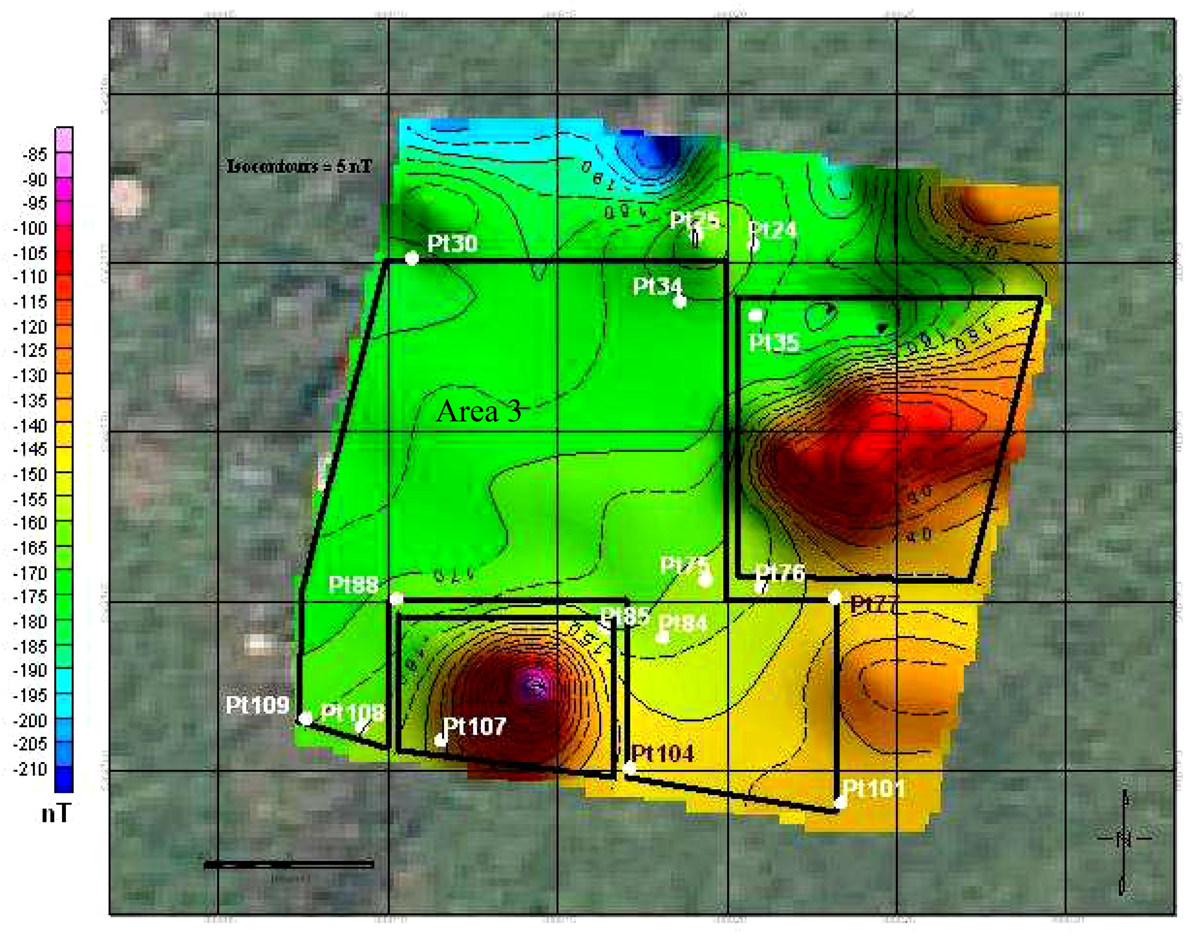
Figure 5 Result of the magnetic cartography of a 20 x 20 m land. Area 3 was chosen to set up the platform. Mapping was carried out using a 20 x 20 m grid. “ptxx” refers to certain points that were used to take the measurements. Area 3 is a square of approximately 13 x 10 m.

The non-magnetic platform was placed on a concrete stone of 3 x 3 m with a good flatness: its maximal slope was assessed to be 3 mm/m or 0.18°, with an average ruggedness equivalent to an uncertainty of 0.15°. The coordinates of its centre were measured in an ellipsoidal system (RGF 93 or Réseau Géodésique Français based on IAG/GRS 80 ellipsoid) with a LEICA GPS receiver used with the RTK (Real Time Kinematic) method (see the signification of acronyms in Table 1). The coordinates of a fixed pillar were also measured to determine a reference direction. Then, these coordinates were transformed into plane coordinates by a Lambert-93 projection, with the help of the software CIRCE of the IGN (the French national geographic institute), and the bearing of this axis was calculated. Knowing the convergence of the meridian at the place of the platform (– 005° 26’ 37.87’’ West), the direction of the true North was deducted. The azimuth shift was projected on the concrete stone with an alidade protractor accurate to 1’ of the angle, which is equivalent to a negligible uncertainty of ± 0.017°. This protractor was used to scale the surface of the concrete block in 10° steps. The accuracy of the graduations was controlled with a GPS receiver used with the RTK method. This procedure yielded the assessment of an average standard deviation or standard uncertainty of 0.26° (according to the definition of the reference BIPM, JCGM 200: 2012) on the absolute positioning of the graduations.

Table 1

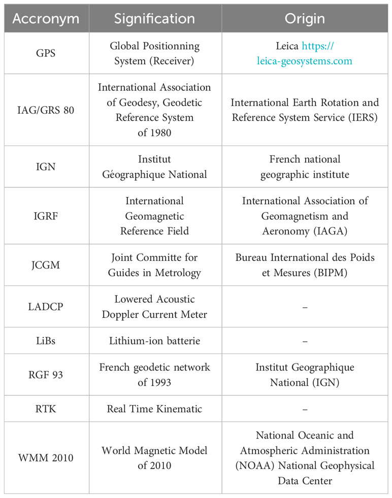
Table 1 List of acronyms used in the text of the publication.

Table 2

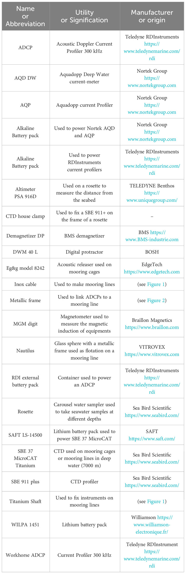
Table 2 List of equipment and accessories tested or used during the experiments.

Before the experiments, the variations of the terrestrial magnetic field were again recorded from 27 September 2022 to 30 September 2022, in order to verify that the magnetic environment had not changed significantly. The record gave daily maximal variations of 60 nT at the maximum and noise of 15 nT peak to peak during measurements. The corresponding maximal relative uncertainty is 0.13% or 0.45° for a 360° rotation. The variation of the magnetic declination was also assessed with the MAGNET software based on the World Magnetic Model WMM 2010 of the NOAA (National Oceanic and Atmospheric Administration) National Geophysical Data Center. On the site of the platform, the annual variation of the declination is 0.19 ± 0.02° in the East direction. At the time of measurements, the declination was – 0.707 ± 0.02° West. This number is adjusted every 9 months in the Excel file used for determining compasses’ magnetic errors, leading to a maximal uncertainty of 0.14° on measurements.

In order to test again the homogeneity of the magnetic field on the platform, the compass of a Nortek Group AQP 600 kHz was calibrated relative to the North by rotating the platform from one graduation to the other. After this, the AQP, which was placed at one end of the platform, was turned in four different directions to measure any differences between the rotation of the platform and the spinning. The results are given in Table 3. The maximal deviation is 0.38° and the average deviation is 0.01°.

Table 3

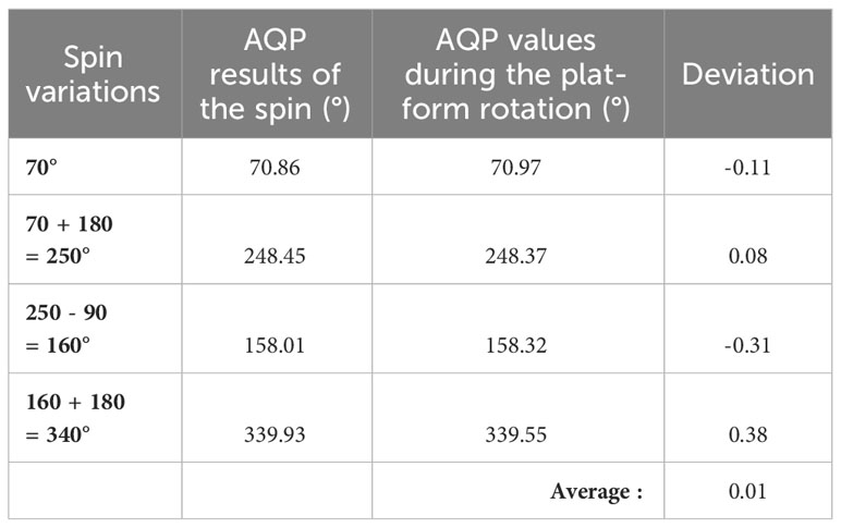
Table 3 Results obtained after the calibration of the compass of an AQP 600 kHz n° 3899 by rotating the platform and comparison with values obtained when this instrument is spun in four directions.

Table 4 gives the details of uncertainties considered to determine reference directions. The square sum of elements such as the slope of the plateau and the knowledge of the magnetic field (earth magnetic field fluctuations, magnetic field dip variations, magnetic anomalies, and magnetic declination) leads to an expanded uncertainty of ± 0.90° on the reference directions used to calibrate the compass, following the recommendations of BIPM, JCGM 100:2008. For information only, the expanded uncertainty of compass calibration is given considering the precisions of the calibrated instruments given in manufacturers’ specifications. The platform can be tilted and the inclination can be measured with a digital protractor (BOSH DWM 40 L) calibrated in a reference laboratory with an uncertainty of 0.12°. Considering the flatness and the ruggedness of the concrete block, the expanded uncertainty on measured reference tilts can be assessed to ± 0.40°. During calibrations, the standard deviation of the polynomial adjustment is added to this number. Table 5 gives the uncertainty budget of a tilt sensor calibration by considering the precision given by the instrument’s manufacturers. According to the guide to the expression of uncertainty in measurement (BIPM, JCGM 100: 2008, § F.2.3.3), the precision given by the instrument’s manufacturers can be considered as a triangular distribution and divided by the root of six to obtain a standard uncertainty on the contributions of instruments.

Table 4

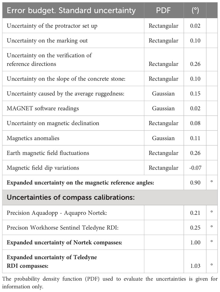
Table 4 Uncertainty budget on the magnetic reference angles and compasses’ calibrations.

Table 5

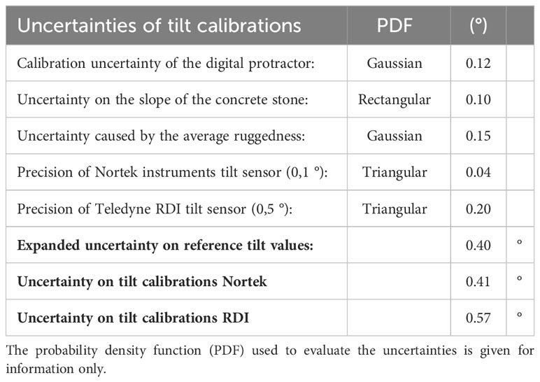
Table 5 Uncertainty budget of tilt sensors calibration.

3 Study of battery packs’ effects

3.1 Explanations of battery magnetism

Batteries are often suspected of producing magnetic anomalies that cause compass measurement errors. Over alkaline batteries, lithium-ion batteries (LiBs) have the advantages of higher energy density, high voltage performance, low self-discharge, no memory effect, superior cycle performance, and good rate performance, but the disadvantage is that it is forbidden in planes because of risks of fire or explosion. Lithium is a paramagnetic substance, that is to say, it is weakly attracted by an externally applied magnetic field and forms internal, induced magnetic fields in the direction of an applied magnetic field. Paramagnets do not retain any magnetisation in the absence of an externally applied magnetic field because thermal motion randomises the spin orientations of their molecules. Magnetic fields interact with electrochemical reactions through variations in electrolyte properties, mass transportation, electrode kinetics, and deposit morphology (Costa et al., 2021). It is the case for LiBs where they can be used to improve performances (Shen et al., 2022). According to Costa et al. (2021), the most widely used materials for anodes are carbon-based, whereas the most widely used materials for the cathode are transition metal-based intercalation materials (layered oxides, spinel oxides, and olivine phosphates) (Hayner et al., 2012). Transition metals, typically Mn, Fe, Co, and/or Ni, allow for the cathodes to be particularly designed to make use of their magnetic properties. It was observed that external magnetic fields resulted in reduced times during the charging and discharging of LiBs due to the paramagnetic nature of lithium ions (Mahon, 2019). It is also possible to measure the battery’s level of charge by tracking changes in the material’s magnetism (Hu et al., 2022).

Lithium batteries are often replaced by alkaline batteries, but alkaline battery packs are known to create perturbations in compass measurements. Alkaline batteries are composed of a cathode made of electrolytic manganese dioxide and carbon. Carbon is mixed with manganese dioxide to ensure good electrical conduction. This cathode is in contact with a so-called “can” surface, made of steel and used as a current collector. The anode is inside the cylindrical cathode. It is composed of layers of pure zinc powder and separated by rings. Inside the anode, a brass pin is used as a current collector. The cathode is protected by either a metal or plastic jacket (Schumm, 2023). Manganese exhibits ferromagnetic properties (it can be attracted by a permanent magnet), but manganese dioxide is a paramagnetic compound. The spin magnetic moment of the electron contributes to the overall paramagnetism of the atoms or molecules. Zhou et al. (2018) supposed that impurity ions/molecules and vacancies are the main factors that contribute to the magnetic performance of δ-MnO₂ although the layer structure is thought to be an origin of ferromagnetic interaction, but the steel case of alkaline batteries can be ferromagnetic and could also explain the observed effects.

3.2 Measurements made on the effects of battery packs

For all the measurements made, the current meter was mounted in the tripode cage. For the first measurements made to test the effects of battery packs, a Nortek Group Aquadopp DW (AQD) was used. The AQD was calibrated at first without a battery pack (it was powered thanks to the cable used to extract data). The obtained maximal error and peak-to-peak errors were low but greater compared to Nortek specification (± 2°): - 3.1° and – 2.7°, respectively (see the AD3CAB curve of Figure 6). A second calibration was made with a reference de-magnetized alkaline battery pack. The magnetic flux density or magnetic induction of battery packs was measured with a small MGM digit magnetometer (see https://www.braillon.com). According to the manufacturer’s specifications, this instrument has an accuracy of ± 2% of the displayed value. The measured magnetic induction of this reference pack is 0.3 G (3 x 10^-5 T). This pack did not modify the response of the compass as can be seen in Figure 6 (curve AD3B00_CAP).

Figure 6

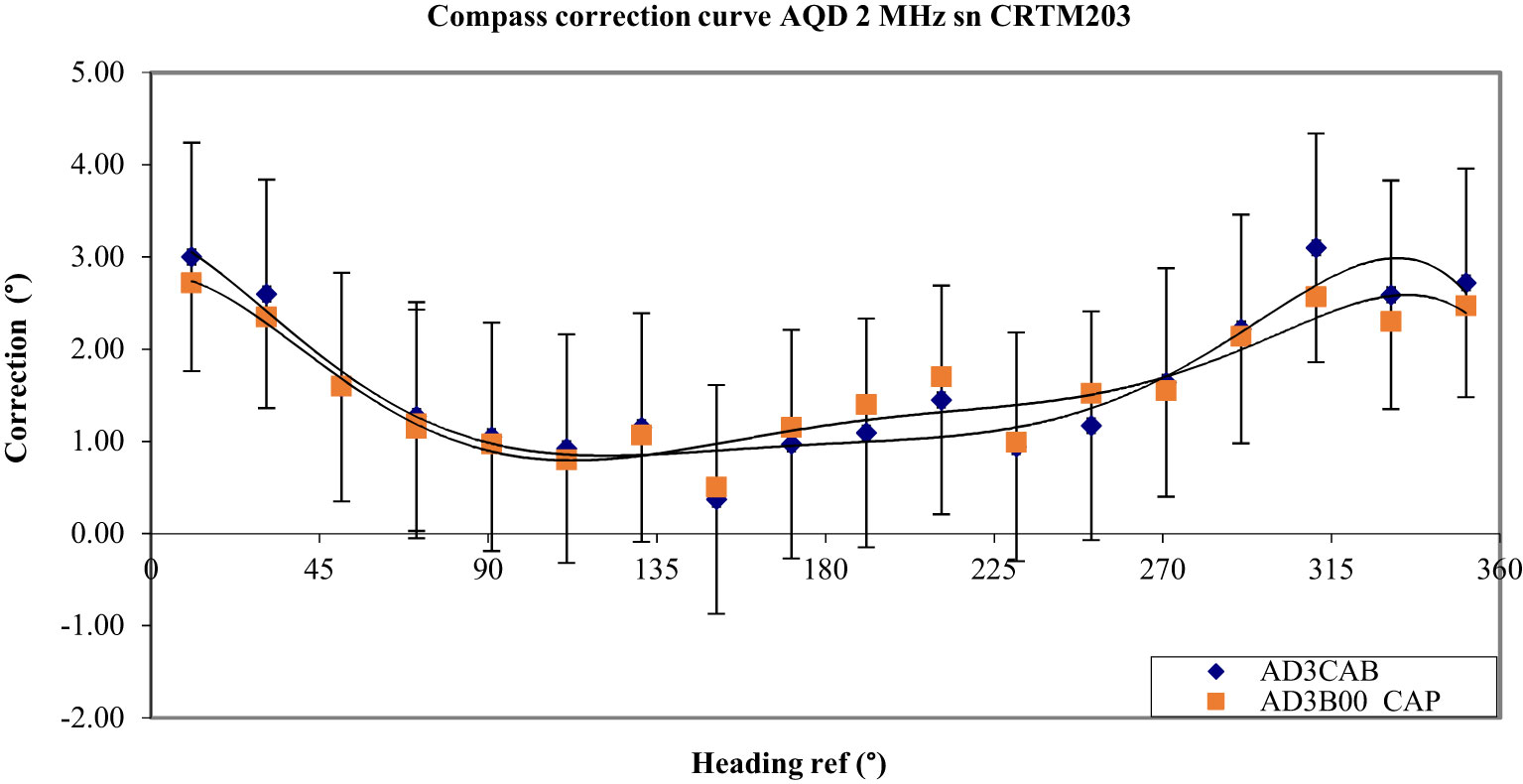
Figure 6 Initial calibration of the ADQ (AD3CAB) and response with a demagnetized battery pack (AD3B00_CAP).

The demagnetized battery pack was then replaced by an alkaline double pack Nortek 034100104 LSA, 13.5 Vdc/7.4 Ah/100 Wh, KW: 49/20, OFL: 08723. This pack was at first oriented to the North and secondly was oriented to the South in the AQD. The errors obtained were largely superior to the AQD specification of 2° in the two cases (12.8° for the maximal error and 22.3° for the peak-to-peak error) with a 180° phase shift (see Figure 7). This phase shift is very problematic to apply a polynomial correction. The corrections could produce a maximal error of 21.3° which is worse than if no corrections were applied. If the pack is oriented from South to West, a 90° shift is observed and the errors still remain significant: 14.8° for the maximal error and 27.9° peak to peak. After having removed this battery pack from the AQD, the measurement of the magnetic induction of this pack gave a high number: 5.7 Gauss (5.7 x 10^-4 T).

Figure 7

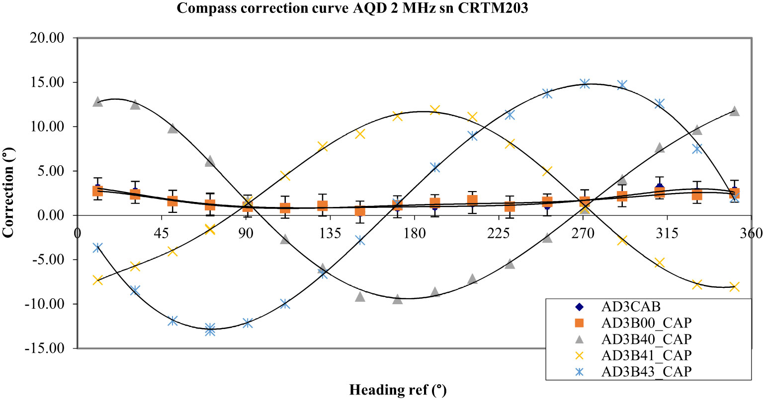
Figure 7 In addition to curves AD3CAB and AD3B00_CAP represented in Figure 6, curves showing the effect of a magnetized battery pack are added. AD3B40_CAP represents the response obtained with a Nortek double alkaline battery pack oriented to the North and AD3B41_CAP, which is the response obtained with the same pack oriented to the South. AD3B43_CAP is the response obtained when the battery pack is oriented to the West.

The next step was to demagnetize it with a BMS demagnetiser-type DP (see www.bms-industrie.com) and to make another calibration on the platform. Its magnetic induction was then 0.4 G. The measurements showed that the AQD errors were again in the uncertainty of the initial calibration of this instrument (see Figure 8).

Figure 8

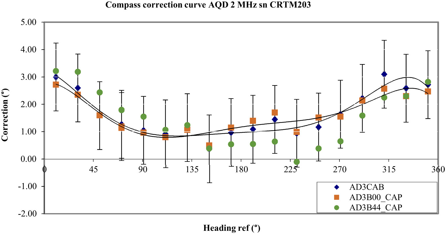
Figure 8 AD3B44_CAP represents the deviations measured after the demagnetisation of the Nortek double alkaline battery pack. Deviations are again in the measurement uncertainty of the initial calibration.

In order to answer the question of whether demagnetized batteries can re-magnetize over time, two current meters Nortek AQD were equipped with small, demagnetized Nortek alkaline battery packs. One of them was stored in its box for 2 months, without being used. The other was turned on, programmed to ping to a low frequency, and also stored in its box for 2 months. Table 6 shows the magnetic inductions and the voltage measured on battery packs before and after 63 days.

Table 6

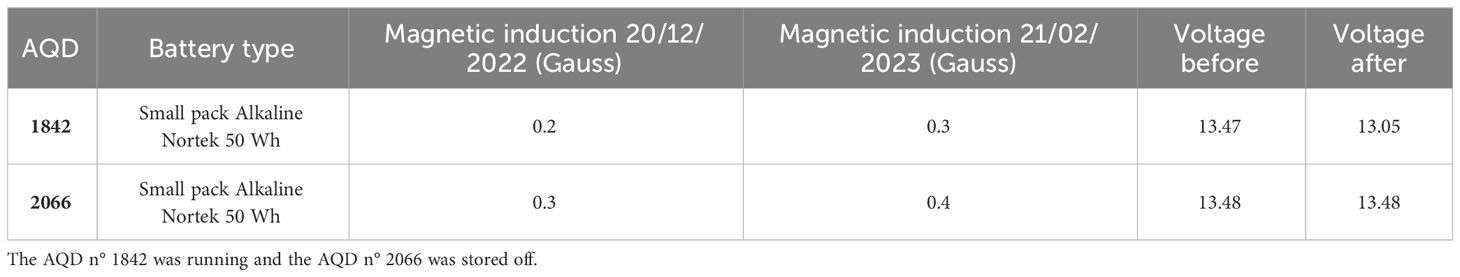
Table 6 Values of magnetic induction and voltage of degaussed battery packs before and after 63 days.

After 63 days, the measured magnetic inductions did not change significantly for the two instruments. The voltage of the AQD n° 1842 decreased as it was collecting data for 63 days. The response of the n° 2066 was the same after 63 days of storage (see Figure 9). The response of the n° 1842 presents a shift, but this shift remains within the initial expanded measurement uncertainty (see Figure 9).

Figure 9

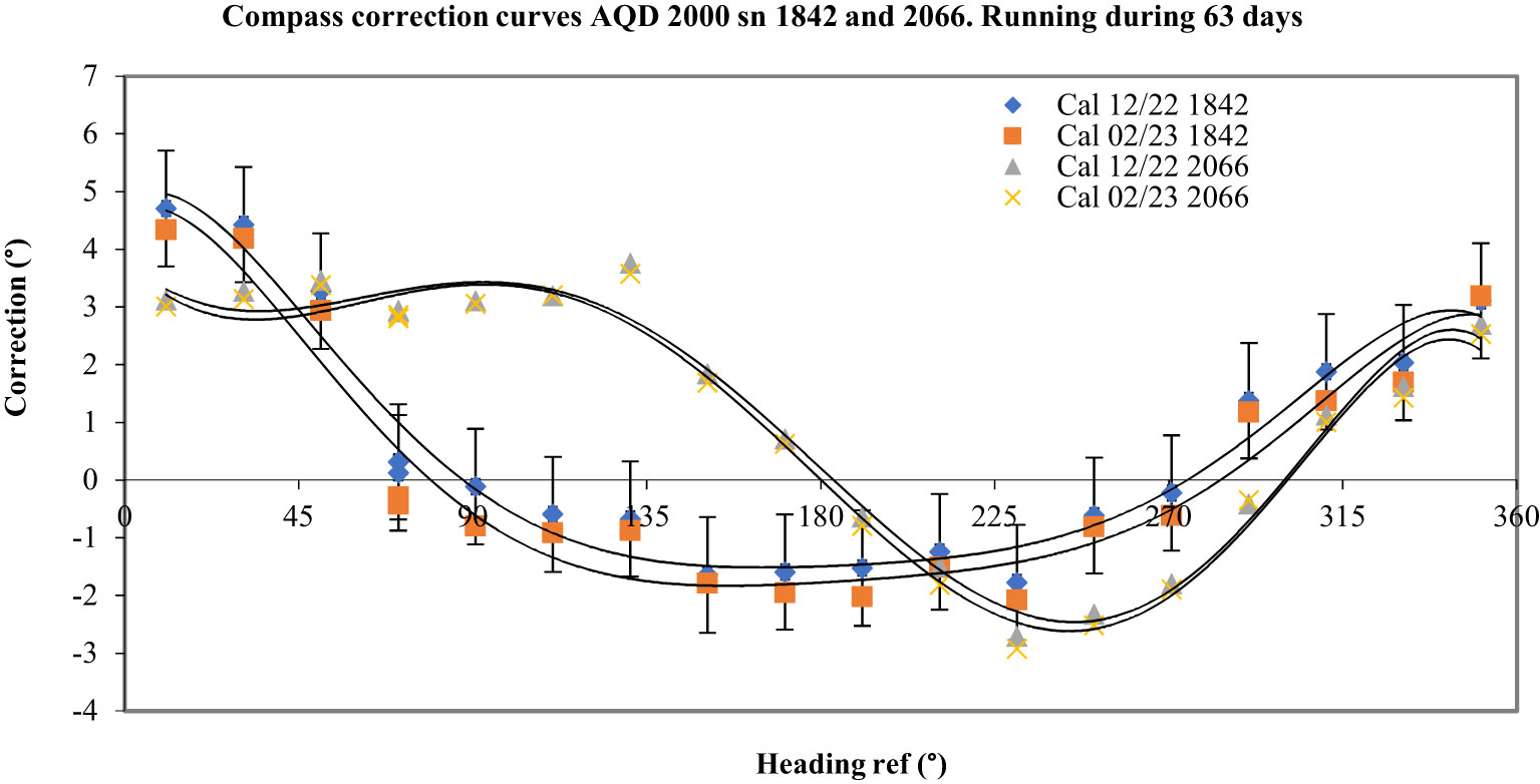
Figure 9 Response of the AQD n° 2066 before and after 63 days of storage without being used and the response of the AQD n° 1842 before and after 63 days running to a low ping frequency.

A small lithium battery pack Williamson, WILPA 1451, 10.8 V/13.5 Ah, was then tested without demagnetising it. Its measured magnetic induction was between 1.0 and 1.1 G. The results showed that it had no impact on the accuracy. The deviations were in the expanded uncertainty of the initial calibration (see Figure 10). A second battery pack added to the first one modified and slightly increased the deviations, but they remained again in the expanded uncertainty. These results demonstrated the lower effect of lithium-ion batteries on compass measurements.

Figure 10

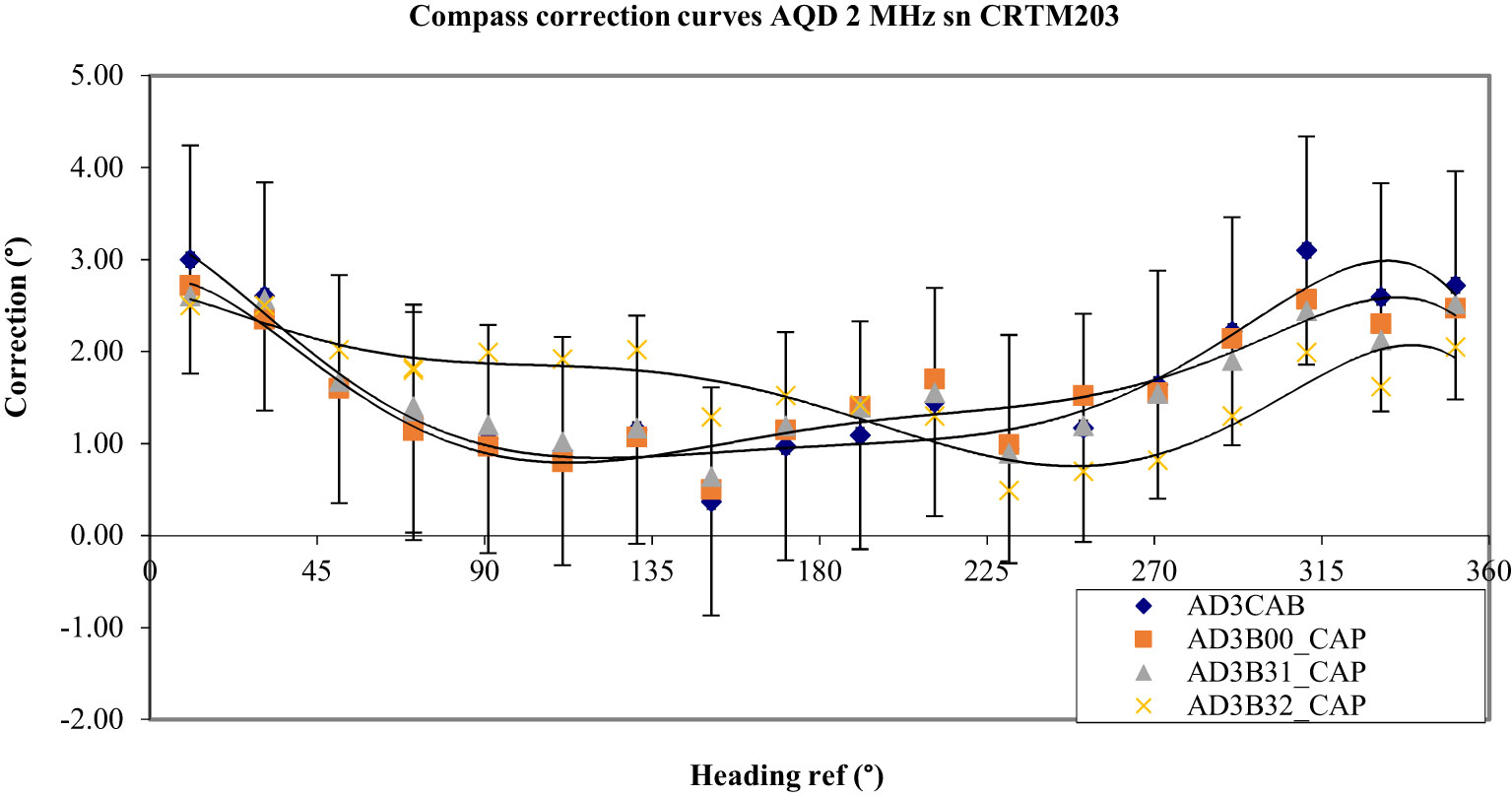
Figure 10 AD3B31_CAP represents the deviations obtained with a battery pack WILPA 1451. AD3B32_CAP shows the deviations obtained by adding a second battery pack WILPA 1451.

Measurements were also made with a Teledyne RDI Workhorse ADCP 300 kHz (sn 1465). This instrument was also mounted on the tripode cage and its horizontality was adjusted. Its response was recorded without a battery pack inside at first and secondly with an RDI alkaline demagnetized battery pack (measured induction: 0.4 to 0.7 G or 4 x 10^-5 to 7 x 10^-5 T). Results show that its compass presents significant angular errors (between 0.9° and 10.5°; 9.6° peak to peak). With the battery pack, errors increase slightly up to 11.0° peak to peak (see Figure 11).

Figure 11

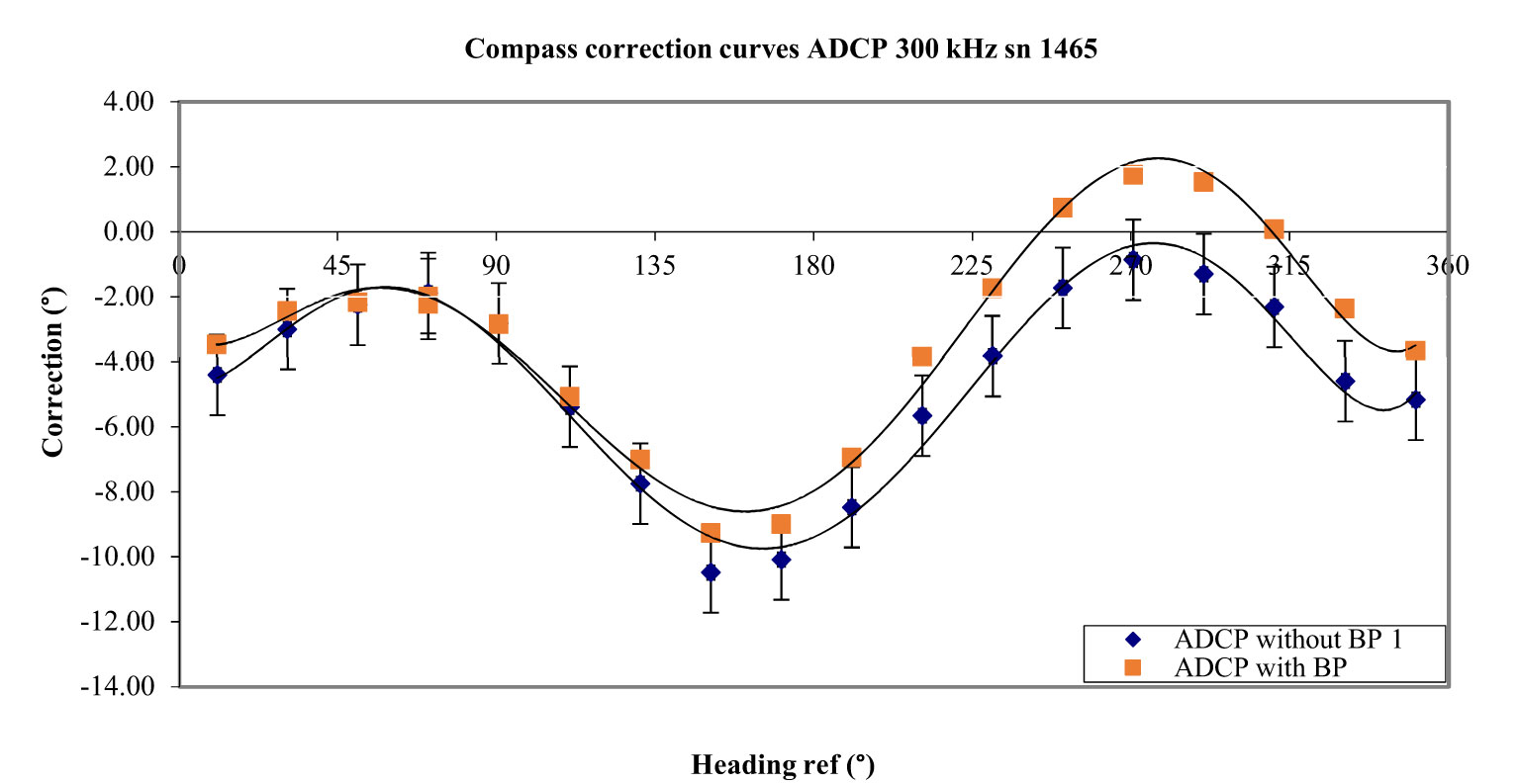
Figure 11 Response of the ADCP sn 1465, without and with a demagnetized battery pack.

These measurements show the low impact of lithium batteries and the significant impact that alkaline batteries can have on the accuracy of compasses. They also show the need to use a demagnetiser before inserting them in current meters.

4 Results of experiments made with mooring accessories

In addition to the batteries, other elements located close to the current meters can generate disturbances in the magnetic field. Some of these have been tested.

The first one is a titanium shaft used in mooring lines to support CTD Sea Bird Instruments SBE 37 MicroCAT (titanium). Used alone, this shaft made of non-magnetic stainless steel has no impact on results. The measured deviations are superimposed to the deviations obtained during the calibration of the AQD without a battery pack (Figure 1).

The second tested accessory is a CTD SBE 37 MicroCAT fixed on the shaft, without a battery pack at first (Figure 1). The errors obtained are very large and on the order of magnitude of the errors obtained with the Nortek double battery pack-oriented West: peak to peak error 26.8°, maximum error 14.8°. Adding in the SBE 37, a lithium battery pack type SAFT LS-14500, 3.6 V/2.6 Ah, slightly reduces the amplitude of the error (see Figure 12).

Figure 12

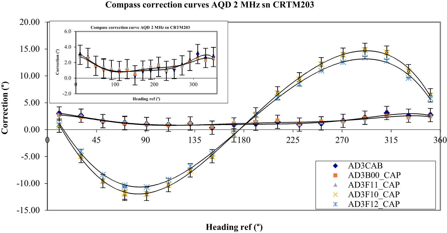
Figure 12 The curve AD3CAB represents the initial calibration of the AQD without a battery pack. The points of this curve are partially covered by the measurements AD3B00_CAP which represent the deviations obtained with a demagnetized battery pack and AD3F11_CAP which represents the deviations obtained with a titanium shaft close to the AQD. The effect of this accessory is completely neglectable. The curve AD3F10_CAP represents the deviations obtained with an SBE 37 MicroCAT fixed on the shaft close to the AQD. The curve AD3F12_CAP corresponds to the same configuration but with a lithium battery pack inside the SBE 37.

The third tested accessory is a part of the inox cable (1.5 m) used on mooring lines and an accessory called ‘clamp’ is used for linking the current meter to the mooring line (see Figure 1). An SBE 37 MicroCAT is also linked to the line, but in this configuration, it is located between 40 and 80 cm higher than the AQD (see Figure 2). Results show that the peak-to-peak error is 11.8° and the maximum error introduced by this assembly is 7.4°. The inox cable has no effect on the compass accuracy, and as expected, the distance between the SBE 37 and the AQD reduces the magnitude of errors.

The fourth tested accessory is a metallic frame that is generally used to fix Workhorse ADCP on a mooring line by means of two metallic collars. The two metallic collars were screwed on the ADCP, but as it was not possible to fix the frame on the nut-and-bolt system, it was just placed on the ADCP (see Figure 3). The ADCP contained the demagnetized battery pack. Results showed that the frame slightly decreased the amplitude of the error curve (See curve ADCP+BP+Frame of Figure 13).

Figure 13

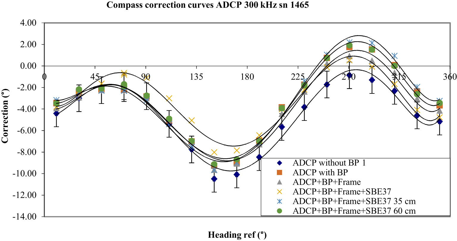
Figure 13 Response of the ADCP sn 1465 in the metallic frame and results obtained with the SBE 37 placed close to the ADCP and then 35 cm and 60 cm higher than the ADCP.

To complete this test, a Titanium SBE 37 made for deep water (7000 m) was placed close to the ADCP (as in Figure 1) and its metallic frame. This SBE 37 contained a lithium battery pack SAFT. Results showed an increase in errors between 50° and 190° and a decrease between 200° and 360°. The peak-to-peak error was less than that obtained with the frame (8.5°). The centre of the SBE 37 was then placed 35 cm higher than the ADCP (Figure 2). Results showed a substantial increase in errors between 200° and 360° and a peak-to-peak error of 11.9°. When the SBE 37 was moved 60 cm higher, the response was almost the same, however, with a small decrease between 200° and 360°.

To simulate the effects of the metallic frames of the elements of a mooring line, the fifth tested element is the metal frame of a 40 cm in diameter glass sphere Nautilus used as flotation. The metallic frame of this sphere was placed 25 cm above the head of the ADCP equipped with its holding frame used on a mooring line. The results show no significant change in the amplitude of errors.

The last tested element is an acoustic releaser Eg&g (EdgeTech) model 8242 placed 86 cm under the ADCP at first (see Figure 4). The releaser had a magnetic induction of 0.1 to 1.1 G according to the position of the magnetometer on this instrument. Results showed an increase in errors (1.7° max.) in the range of 0° to 170° and a decrease in the same amplitude in the range of 190° to 350° (see Figure 14). After these measurements, the distance between the two instruments was reduced to 65 cm. Unexpectedly, no significant change was measured (see Figure 14).

Figure 14

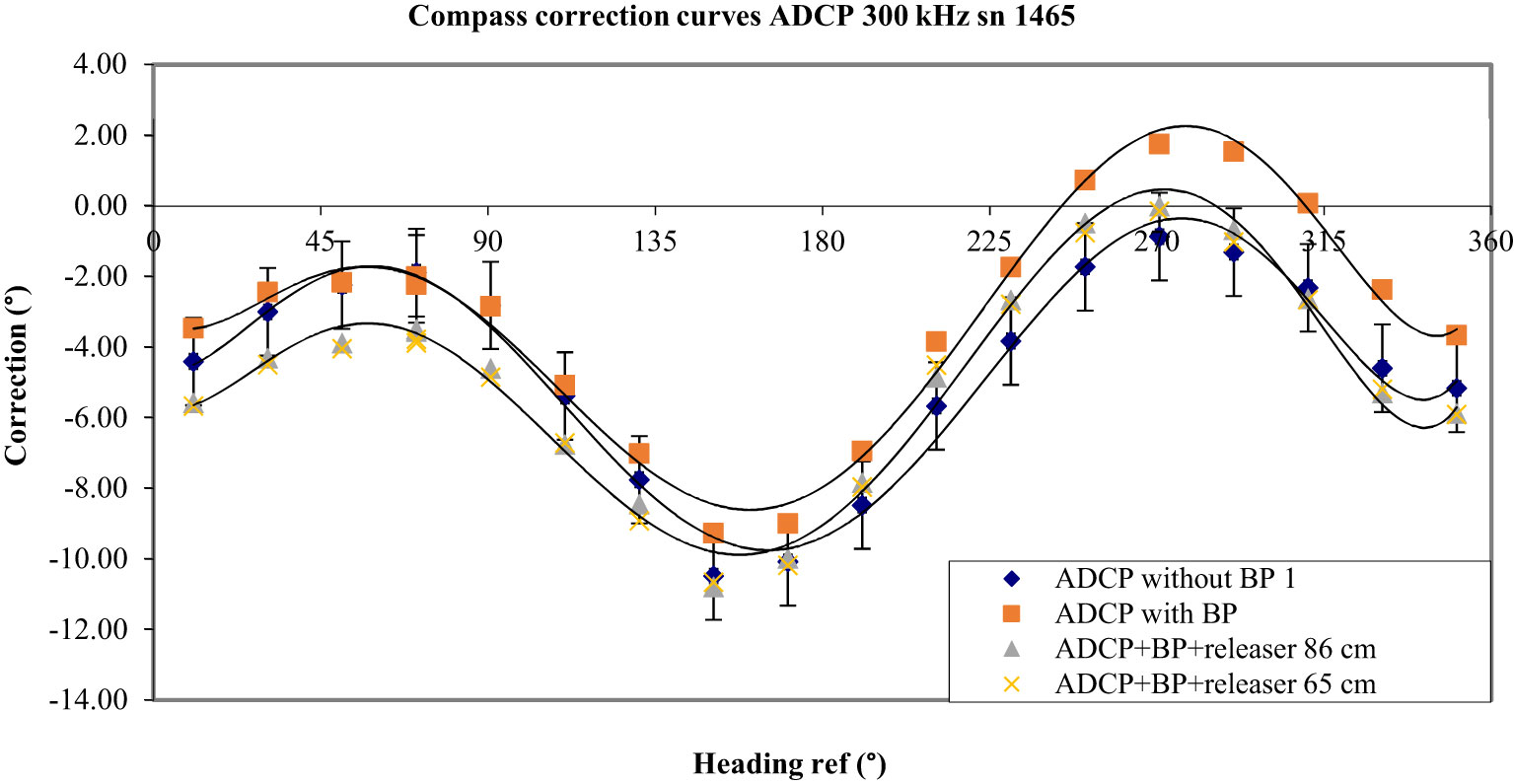
Figure 14 Results of the test made with an acoustic releaser placed 86 and 65 cm under the ADCP.

5 Test of a LADCP configuration

ADCPs are often associated with a CTD profiler fixed on a rosette of sampling bottles in a configuration called LADCP (Lowered Acoustic Doppler Current Profiler). It is the case, for example, of the campaign MedSHIP described by Schroeder (2021). We tested the effect of an 8-bottle rosette equipped with an SBE 911 plus CTD profiler, a Teledyne RDI external battery pack, and an altimeter PSA 916D, on the ADCP sn 1465. At first, the ADCP was fixed to the top of the rosette to simulate an ‘uplooker’ or ‘slave’ LADCP configuration. It was held to the rosette by a stainless-steel clamp. It was set to be horizontal and oriented so that its main marker was correctly aligned with the axis of the platform (see Figure 15). No significant change was recorded compared to deviations obtained with the ADCP alone, equipped with its battery pack (Figure 16).

Figure 15

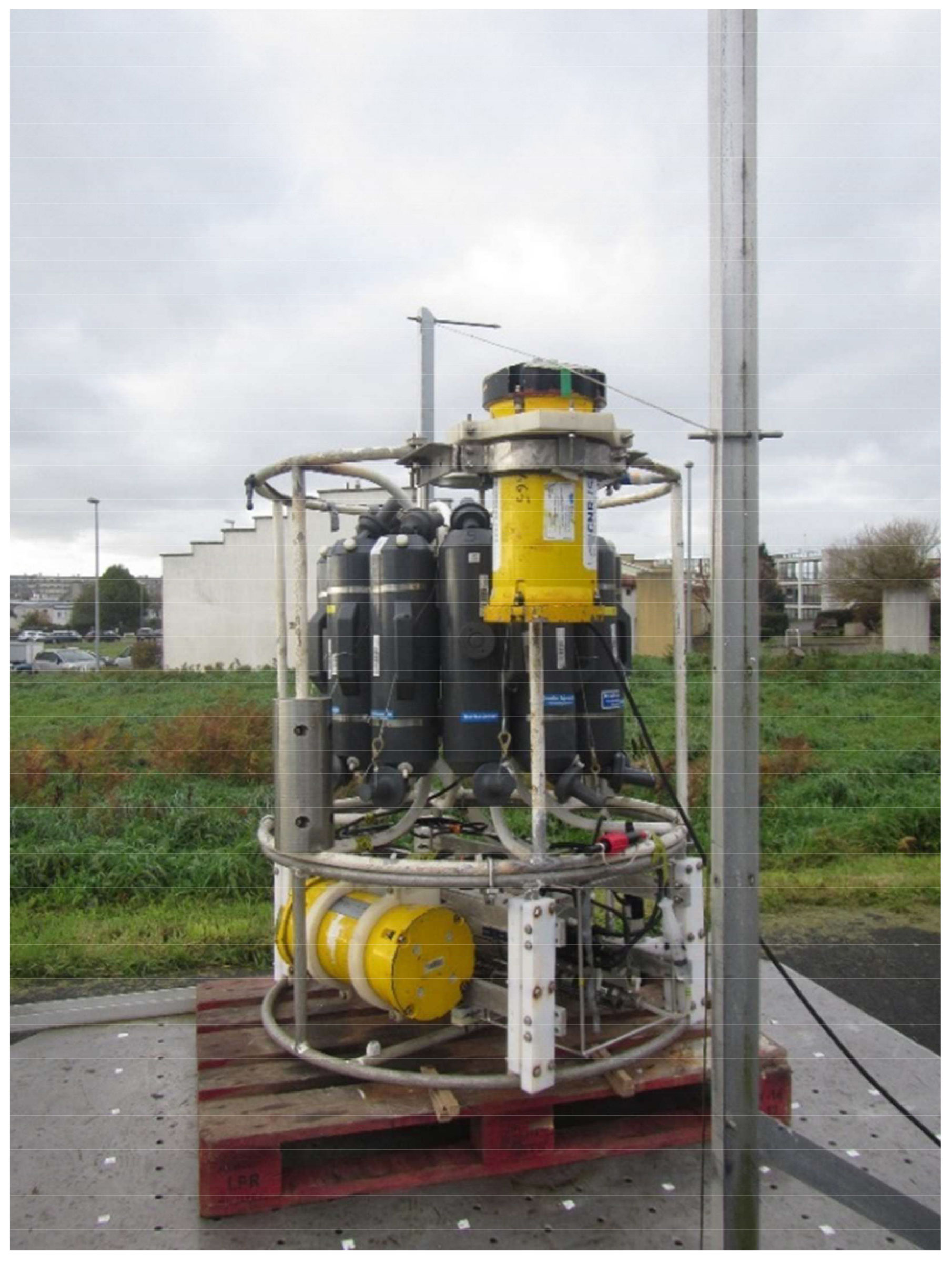
Figure 15 LADCP configuration with the ADCP at the top of the rosette.

Figure 16

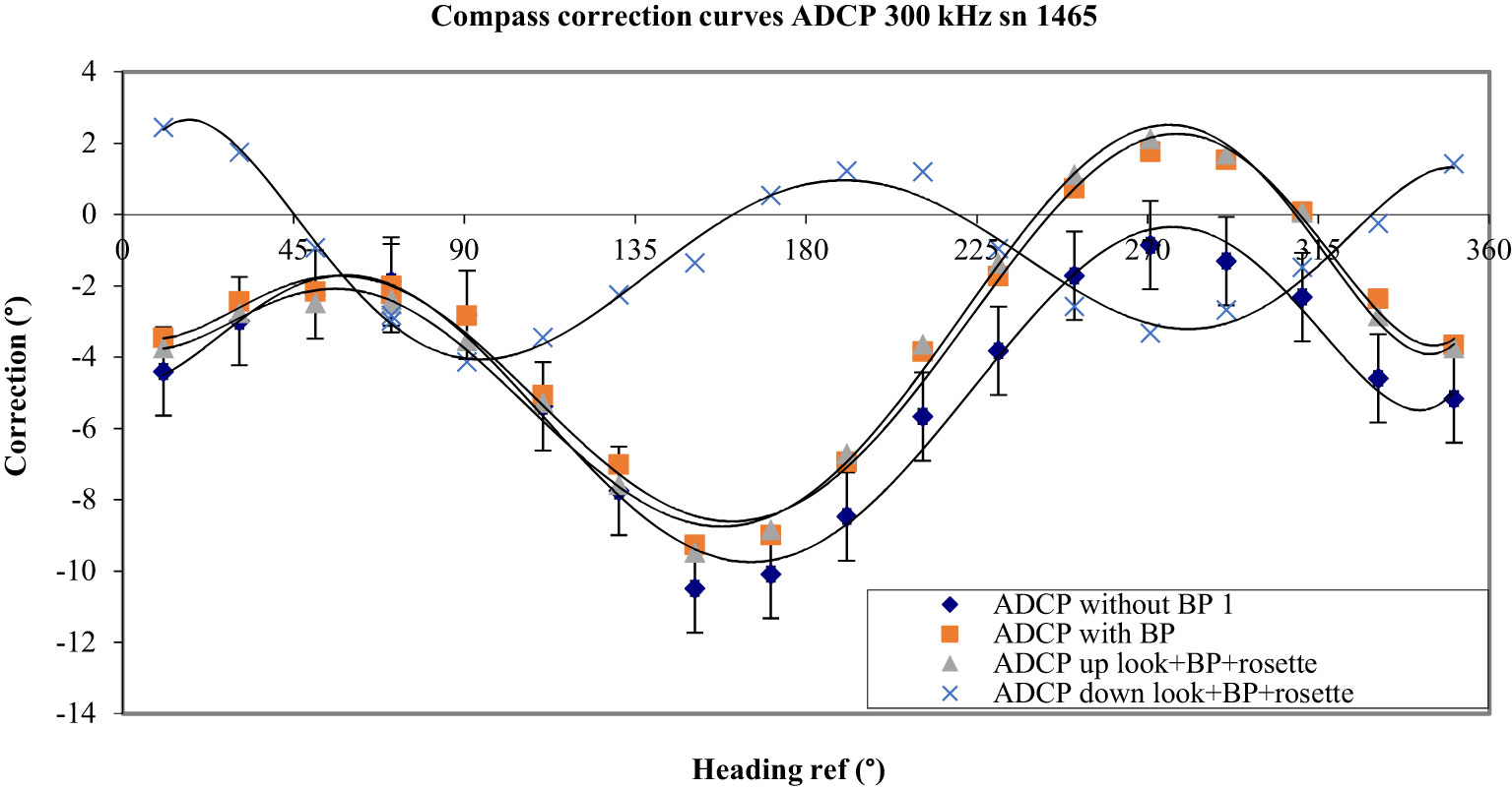
Figure 16 Results obtained with the LADCP configuration. Green triangles represent the deviations obtained with the ADCP fixed at the top and looking up, and the blue crosses show the deviations obtained with the ADCP fixed at the bottom and looking down.

After this first test, the ADCP was clamped at the bottom of the rosette, looking down as in a “master” LADCP configuration. The results obtained were completely different. The peak-to-peak error was reduced (11.6° when clamped at the top and 6.6° when clamped at the bottom) and the curve was better centred to the horizontal axis (see Figure 16). This result was as much surprising that the CTD hose clamp that was at 52 cm of the ADCP had a very large magnetic induction of 14 G (1.4 x 10^-3 T). Several screws that were one meter away from the compass were also magnetized, but the external battery pack that was 22 cm away showed a small magnetisation (0.05 Gauss).

These tests show how difficult it is to model and predict the effects that the various components of a cage or mooring line can have on the accuracy of current meter compasses.

6 Theoretical background and elements about methods to correct compass deviation

Compasses are sensitive to disturbance from magnetic fields created by metallic materials in the vicinity (Gebre-Egziabher et al., 2001; Fang et al., 2011), as demonstrated by measurements made on the platform. Ferromagnetic materials are considered to be soft if they exhibit a low induced field when exposed to an external magnetic field and hard if they exhibit a high residual induced field permanently (Le Menn et al., 2014). Iron, cobalt, and nickel alloys are typically hard magnetic materials that create permanent magnetic fields. Soft magnetic materials generate magnetic fields only under the action of another field. This is the case with lithium. Soft magnetic materials can distort a uniform magnetic field and generate errors.

Electronic compasses are made up of three orthogonal magnetometers. They measure induced flux densities M_x, M_y, and M_z. Soft magnetic materials distort a uniform magnetic field and generate errors that can be described by a 3 x 3 matrix $\underset{\_}{C_{si}}$. Hard magnetic materials add a constant magnetic field component along each axis and generate offsets $\delta {\overrightarrow{B}}^b$ that shift the output of the sensors. Compasses’ magnetometers can be not orthogonal and misaligned. Magnetometers can also have differences in sensitivities. These sources of errors can be described by the error matrix $\underset{\_}{C_m}$ and $\underset{\_}{C_{sf}}$, respectively. If $\underset{\_}{h_m^b}$ is the projection of the magnetic field vector measured by the compass in its body axis, and h^b is the true magnetic field, according to Fang et al. (2011):

$\begin{array}{ll}\underset{\_}{h_m^b}=\underset{\_}{M}\underset{\_}{h^b}+\underset{\_}{\delta {\overrightarrow{B}}^b}+\underset{\_}{n}& (1)\end{array}$

where $\underset{\_}{M}=\underset{\_}{C_m}\underset{\_}{C_{sf}}\underset{\_}{C_{si}}.\underset{\_}{n}$ is the measurement noise of the three magnetometers.

In addition to relation (1), in 2011, Fang et al. proposed a method for correcting compasses based on the fact that the error model of a magnetic compass is an ellipsoid. The locus of the true magnetic field $\underset{\_}{h^b}$ used in Equation 1 is spherical if the centre of the compass remains stationary and only the direction is changed, giving a constant magnitude field so that the locus of the perturbed, measured field $\underset{\_}{h_m^b}$ is an ellipsoid. The autocalibration procedures proposed by the current meter manufacturers are based on these facts. According to Fang et al. (2011), $\underset{\_}{h_m^b}$ can be expressed with the equation of a quadric:

$\begin{array}{ll}\parallel h^b{\parallel }^2={\left(h_m^b\right)}^T{\underset{\_}{Ah}}_m^b-2\underset{\_}{\delta {\overrightarrow{B^b}}^{T}A{h}_m^b}+b^T\underset{\_}{A\delta \overrightarrow{B^b}}+\underset{\_}{\tilde{n}}& (2)\end{array}$

where $\underset{\_}{A}={\underset{\_}{G}}^T\underset{\_}{G}$, $\underset{\_}{G}={\underset{\_}{M}}^{-1}$ and $\underset{\_}{\tilde{n}}=2{\left({\underset{\_}{h}}_m^b-b\right)}^T{\underset{\_}{G}}^T\underset{\_}{G}\underset{\_}{n}+{\underset{\_}{n}}^T{\underset{\_}{G}}^T\underset{\_}{G}\underset{\_}{n}$. Even though $\underset{\_}{n}$ may be zero mean and Gaussian, the mean value of $\underset{\_}{\tilde{n}}$ may not.

Equation 2 can be transformed into the general conicoid equation in the 3D space. A constraint least squares method can be used to determine the coefficients of this conicoid by taking measurements on a non-magnetic platform to position the compass at different angles in the 3D space. Fang et al. (2011) showed that this was an effective absolute calibration method for compasses, but to date, it cannot be applied to existing current meters and profilers because the user’s software does not provide the values measured by the individual magnetometers.

However, since the introduction of iron ships in the 19th century, researches were carried out to correct errors in magnetic compass measurements. The relations used to correct compasses were derived from studies carried out by Siméon Denis Poisson in 1824 (famous for his equation which describes the dependence of electric potential on charge density). The hard iron correction formula can be well represented by a one-cycle model (Denne, 1998) given by equation (3):

$\begin{array}{ll}\delta (\Omega )=A+Bsin(\Omega )+Ccos(\Omega )& (3)\end{array}$

where δ(Ω) is the heading-dependent compass error; Ω is the compass heading recorded by the instrument; A, B, and C are constants. A is the constant heading offset of the compass. A remains constant on any part of the Earth. B and C represent the effects caused by the hard and soft vertical irons. The complete formulation is due to Evans and Smith. The magnetic course is plotted in Fourier series describe by equation (4):

$\begin{array}{ll}\tan (\delta )=\frac{a+bsin(\Omega )+ccos(\Omega )+dsin(2\Omega )+ecos(2\Omega )}{1+bsin(\Omega )-csin(\Omega )+dcos(2\Omega )-esin(2\Omega )}& (4)\end{array}$

where a, b, c, d, and e are constants to determine. For deviations less than 20°, relation (4) was simplified by Smith following his theory of the compensation derived from the fundamental relations of Poisson (Bourbon, 2002). Smith’s relation is:

$\begin{array}{ll}\delta (\Omega )=A+Bsin(\Omega )+Ccos(\Omega )+Dcos(2\Omega )+Esin(2\Omega )& (5)\end{array}$

It is a two-cycle equation that considers hard and soft iron errors. Compared to relation (3), coefficient D represents induced magnetism from symmetrical or horizontal soft iron and E from asymmetric soft iron (Denne, 1998). E can be zero if the soft irons are symmetrical to the compass. In the case of a ship that sails by changing direction and magnetic latitude, the terms B and C may take slightly different values. However, this technique is the only one known to correct compass errors. It was used in 2010 to correct a diver navigation system Cobra-Tac (Teledyne RD Instruments) based on acoustic Doppler velocity log (DVL) technology that uses dead reckoning to compute displacements from a known starting point (Hench and Rosman, 2010). It was also used in 2021 to determine the residual deviations of electronic compasses used for navigation (Androjna et al., 2010) and it was used on all the ships (cargo, tankers, and container ships) even when they were equipped with gyro-compasses (Androjna et al., 2010).

This technique can be used to correct current-meters and current profilers’ compasses in their using configuration. From the Equation 5, the corrected heading angle Ω_cor expressed in degrees is given by the relationship (6):

$\begin{array}{ll}{\Omega }_{cor}=[\Omega +\text{A}+\text{B}.sin(\Omega )+\text{C}.cos(\Omega )+\text{D}.cos(2\Omega )+\text{E}.sin(2\Omega )].180/\pi & (6)\end{array}$

Coefficients A, B, C, D, and E can be determined by a least square technique. Figure 17 gives an example of the application of this technique to a Nortek AQD 2000. The standard deviation of the fitting’s residuals can be used as the instrument and measurement part, to calculate the uncertainty of the calibration. In this example, the expanded uncertainty is 1.14° with a probability of 95%.

Figure 17

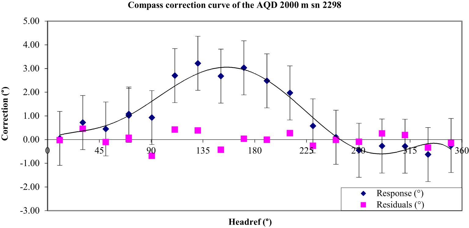
Figure 17 Result of the compass calibration of the AQD 2000 n° 2298. The blue squares represent the corrections obtained on the calibration platform and the purple squares are the residuals after applying the relation (6).

A simple polynomial relation of degree 6 can be sometimes used too when the software used to process the data does not allow the relationship (4) to be programmed. In this case, Ω_cor is obtained by the relationship (7), where Ω is expressed in °:

$\begin{array}{ll}{\Omega }_{cor}=\Omega +\text{A}+\text{B}.\Omega +\text{C}.{\Omega }^2+\text{D}.{\Omega }^3+\text{E}.{\Omega }^4+\text{F}.{\Omega }^5+\text{G}.{\Omega }^6& (7)\end{array}$

where A, B, C, D, E, F, and G are coefficients obtained by a least square technique. In the case of the AQD 2000 n° 2298, the expanded uncertainty obtained is 1.66°, showing that the relationship (6) gives a better result. However, for some instruments, the relationship (7) gives better uncertainties. That can be probably explained by the fact that for these instruments, the response curve is not only a function of the hard and soft iron errors but also of the compass electronic interface that affects the response.

The mastered magnetic environment of the calibration platform offered an opportunity to test the Nortek autocalibration procedure described in Nortek (2017), pages 74-75. It was applied in the configuration of Figure 1 where the AQD was on the tripode cage and an SBE 37 was fixed on a shaft at the same height (Curve AD3F10_CAP of Figure 12). The AQD was equipped with a demagnetized Nortek double battery pack. The autocalibration consists of:

- Using Nortek software section ‘compass calibration’.

- Rotating the entire system 360° horizontally and slowly (60 s per rotation) around the Z-axis of the instrument. The software must show a circle more or less perfect according to the magnetic environment and the regularity of the rotation.

- Clicking ‘Done’ to use the obtained calibration values in the instrument as a new compass setting.

The software gives an estimated maximum error after using this procedure to determine if its application was correct. Figure 18 shows that the residual errors are in the calibration expanded uncertainty we had after the initial calibration with a demagnetized battery pack inside the AQD (max. error of 2.5° and peak-to-peak error of 2.0°), but it remains a shift of 1.6°. That could be explained by the fact that the mean value of $\underset{\_}{\tilde{n}}$ that appears in Equation 2 may not be zero even though $\underset{\_}{n}$ may be zero (Fang et al., 2011). However, when applied in a known magnetic environment, this procedure gives a sufficiently good result.

Figure 18

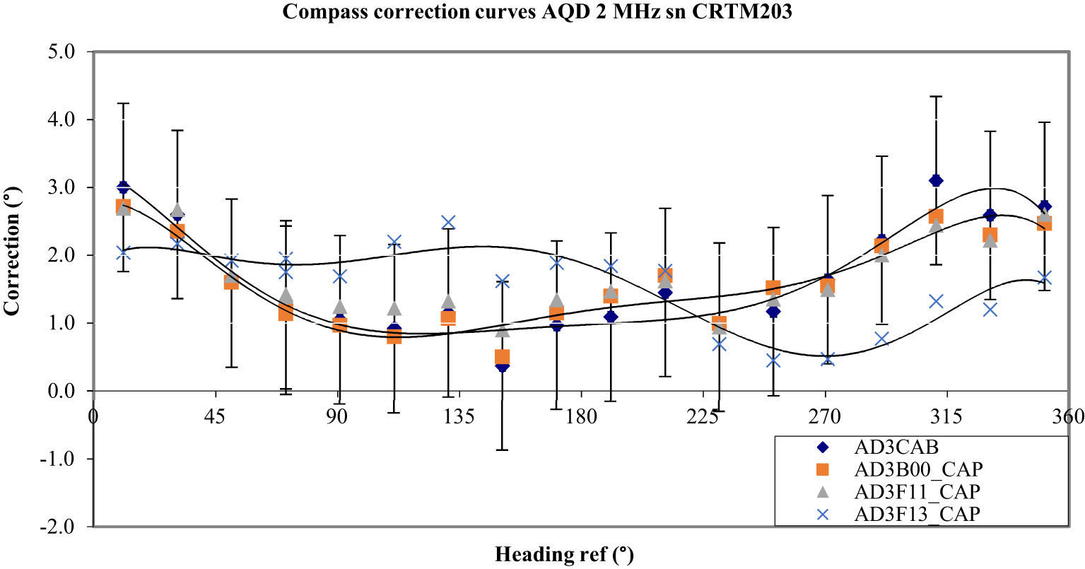
Figure 18 Curve AD3F13_CAP shows the residual errors obtained after applying the Nortek autocalibration procedure. The error of Figure 12 is completely reduced but with a remaining small shift.

The effectiveness of the Teledyne RDI autocalibration procedure was also tested (see RD Instrument, 2005). The option “Calibration for a single tilt orientation (single + double cycle)” was chosen. This option was intended to reduce hard and soft iron errors.

A first trial was made without a battery pack in the ADCP. The measurements made after applying the procedure showed no significant improvement in the reduction of errors. The peak-to-peak correction was worse (9.6° before and 13.8° after the autocalibration). The same autocalibration procedure was applied to the ADCP equipped with a battery pack. Once again, the results did not show significant improvements although the peak-to-peak error was slightly smaller (11.0° before and 10.2° after autocalibration) (see Figure 19). These results do not allow conclusions on the efficiency of the autocalibration algorithm of the Teledyne RDI compasses.

Figure 19

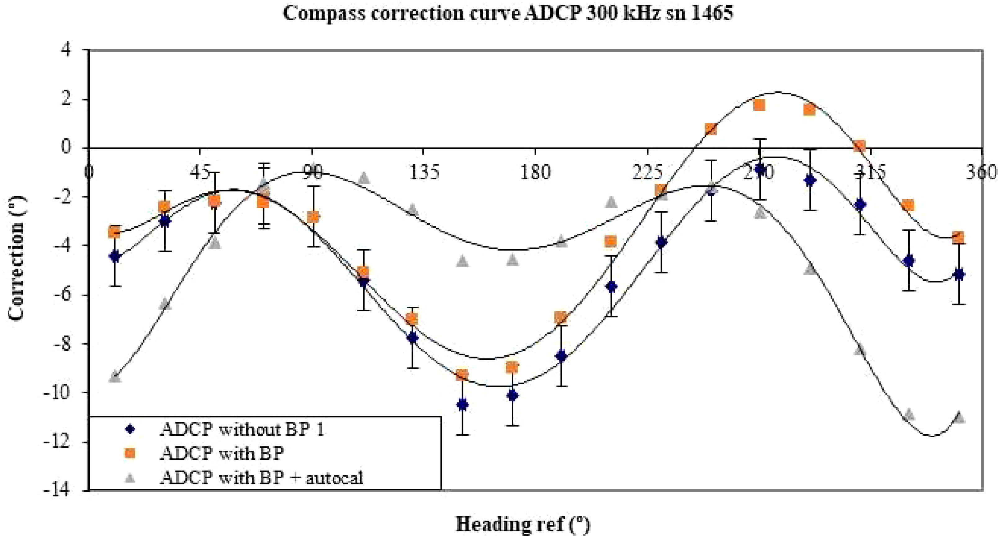
Figure 19 Results obtained before and after application of the autocalibration procedure on the ADCP equipped with a battery pack.

7 Conclusion: opening the way to best practices

Experiments have been made on the Eulerian standalone instruments of Nortek Group and Teledyne RDI using the Doppler effect and a magnetic compass to measure the velocity and the direction of sea currents. The goal was to detect and measure the influence of various elements that compose mooring cages or mooring lines on the compass measurements thanks to experiments made on Shom’s calibration platform.

Among elements tested, alkaline batteries can induce very large errors (as much as 27.9° peak-to-peak measured). The phase of the error response curve varies according to the orientation of the battery pack inside the current meter, making corrections unavailable (see Figure 7). The solution to adopt consists of demagnetising the battery packs with a 50 Hz demagnetiser before they are introduced in the instrument. Measurements have shown that the demagnetisation remains for at least 2 months and probably a much longer time when a current meter is stored in its box. Measurements have also shown that the demagnetisation remains for at least 2 months when the current meter makes measurements.

Regarding lithium batteries, they cannot be magnetized theoretically, but they can generate a magnetic field in the presence of a magnetic field. The measurements have shown that using one battery pack did not change the response of the compass, but using two lithium packs can lead to a phase shift of the response curve. Because of this unforeseeable phenomenon, alkaline batteries should be preferred to lithium packs so that they can efficiently be demagnetized as demonstrated with different measurements.

Experiments made on different objects that can be in the vicinity of current meters have also shown that they can perturb compass measurements as, for example, CTD SBE 37 fixed on a shaft close to an AQD. The influence of a magnetic field being inversely proportional to the square distance from its source has shown that when the SBE 35 is at 40 to 80 cm of the AQD, the peak-to-peak error is divided by 44%. Other elements can have an influence such as metallic frames used on mooring lines or clamps and screws used on LADCP cages. If the demagnetisation of these elements is not possible (that has not been tested), the solution is to calibrate the compass with all its surrounding equipment’s in the using configuration, on the platform. A correction polynomial can be calculated to fit the error curve and to reduce the errors.

Correction formulas exist and they have been used since the 19th century to compensate for compass errors on metallic ships. The Smith formula has been used at Shom since 2012 to correct data recorded by current meters and current profilers. Even if the corrections are not perfect because some coefficients are sensitive to the orientation and the inclination of the magnetic field, it remains one of the best ways to correct compass errors. These corrections can be applied to the instrument calibrated alone or to an instrument with its mooring equipment.

The other way to correct compass errors is to use the autocalibration procedures proposed by the manufacturers. We have tested Nortek Group and Teledyne RDI procedures. When used in a mastered magnetic environment, the Nortek procedure seems to provide good results. For unexplained reasons, the Teledyne RDI procedure did not significantly reduce the errors of the tested profiler. The problem that remains is to be sure of the lack of magnetic anomalies when applying these procedures in an environment where the magnetic field has not been mapped.

These experiments enable us to make general recommendations in measuring the direction of marine currents. When calibrating a current meter compass, at least three elements must be considered:

- The first to master is the magnetic environment. As shown in previous sections, elements such as alkaline batteries or non-magnetic metal parts in the vicinity of the current meter to be tested can cause significant interference. In addition to elements visible on the surface, nearby buried metal elements can also generate magnetic anomalies such as those shown in Figure 5. These anomalies can be detected and sometimes removed using a simple metal detector. In the case when magnetic anomalies are detected and not removed, according to their amplitudes, the calibration must be located within a radius of 1 to 3 meters of the anomaly. This precaution must be taken whatever the correction technique used: either relationship (6) or manufacturer’s autocalibration techniques. A magnetometer with a sensitivity of approximately 0.1 G or better can be used to appreciate the distance where the influence of the anomaly becomes neglectable.

- The second element concerns the current meter’s power supply. Considering the results presented in § 3.2, alkaline batteries are preferable to lithium batteries, provided they are correctly demagnetized before being inserted in the current meter. In this section, it is shown that demagnetisation lasts at least 2 months (and probably longer) under the conditions in which the instruments are stored or used.

- The third element is to take into account the instrumental environment in which the current meter will make its measurements. The calibration must be made with the battery packs that will be used and with the instrumented cage of the mooring or with the elements that will be in the vicinity of the current meter on the mooring line. In the case of LADCP measurements, the current profiler must be fixed on the instrumented carousel water sampler for its calibration.

Apart from problems posed by the magnetic environment close to the compass, it is difficult to use and calibrate compasses in areas close to the North or the South Magnetic Poles. For example, at 700 km from the North Magnetic Pole, the angle that the magnetic field vector makes with the horizontal is 88.2° (Hamilton, 2001). The horizontal component of the magnetic field is too small (< 5000 nT), and the sensitivity of the compass leads to fluctuations and errors in measurements. Fluctuations come also from the variations in pole location that are more sensitive and result in significant changes in magnetic declination. In these areas, compass corrections proposed in this publication should no longer be valid. Other techniques must be used such as gyrocompass to retrieve the direction of instruments or data from nearby geomagnetic observatories associated with reference compass (Hamilton, 2001). However, in most current cases, the general recommendations given previously can pave the way for the development of “best practices” that can be discussed and elaborated with working groups of projects such as MINKE or the IOC (Intergovernmental Oceanographic Commission) Ocean Best Practices community.

Data availability statement

The raw data supporting the conclusions of this article will be made available by the authors, without undue reservation.

Author contributions

ML: Investigation, Writing – original draft. DL: Writing – review & editing. KS: Writing – review & editing. MB: Investigation, Writing – review & editing.

Funding

The author(s) declare financial support was received for the research, authorship, and/or publication of this article. This paper was written in the frame of the MINKE (Metrology for Integrated Marine Management and Knowledge-Transfer Network) Project funded by the European Commission within the Horizon 2020 (2014-2020) research and innovation program under grant agreement 101008724. The development and manufacturing of the calibration platform was funded by the French Naval Hydrographic and Oceanographic Service (Shom).

Acknowledgments

The authors would like to acknowledge the precious help from Fabien Perault (DT-INSU) and Lotfi Radjouh (Shom) during the field experiment and subsequent reporting, as well as the reviewers for their comments, corrections, and improvements of the text.

Conflict of interest

The authors declare that the research was conducted in the absence of any commercial or financial relationships that could be construed as a potential conflict of interest.

Publisher’s note

All claims expressed in this article are solely those of the authors and do not necessarily represent those of their affiliated organizations, or those of the publisher, the editors and the reviewers. Any product that may be evaluated in this article, or claim that may be made by its manufacturer, is not guaranteed or endorsed by the publisher.

References

Alken P., Thébault E., Beggan C. D., Amit H., Aubert J., Baerenzung J., et al. (2021). International Geomagnetic Reference Field: the thirteenth generation. Earth Planets Space 73, 49. doi: 10.1186/s40623-020-01288-x

CrossRef Full Text | Google Scholar

Androjna A., Belev B., Pavic I., Perkovič M. (2010). Determining residual deviation and analysis of the current use of the magnetic compass. J. Mar. Sci. Eng. 9, 204. doi: 10.3390/jmse9020204

CrossRef Full Text | Google Scholar

BIPM, JCGM 100:2008 (2008). Evaluation of measurement data – Guide to the expression of uncertainty in measurement, first edition. Available at: https://www.bipm.org/documents/20126/2071204/JCGM_100_2008_E.pdf/cb0ef43f-baa5-11cf-3f85-4dcd86f77bd6.

Google Scholar

BIPM, JCGM 200:2012 (2012) International Vocabulary of Metrology – Basic and general concepts and associated terms (VIM). 3rd edition. Available at: www.BIPM.org/publications/guides.

Google Scholar

Boldt J. A., Oberg K. A. (2015). Validation of streamflow measurements made with M9 and RiverRay acoustic Doppler current profilers. J. Hydraul. Eng. 142, 2. doi: 10.1061/(ASCE)HY.1943-7900.0001087

CrossRef Full Text | Google Scholar

Bourbon P. (2002). Guide pratique du compas magnétique (Institut Oceanographique), 277 pp.

Google Scholar

Camnasio E., Orsi E. (2011). Calibration method of current meters. J. Hydraul. Eng. 137, 386–392. doi: 10.1061/(ASCE)HY.1943-7900.0000311

CrossRef Full Text | Google Scholar

Costa C. M., Merazzo K. J., Gonçalves R., Amos C., Lanceros-Mendes S. (2021). Magnetically active lithium-ion batteries towards battery performance improvement. Science 24 6, 102691. doi: 10.1016/j.isci.2021.102691

CrossRef Full Text | Google Scholar

de Mendoza F. P., Schroeder K., Langone L., Chiggiato J., Borghini M., Giordano P., et al. (2022). Deep water hydrodynamic observations of two moorings sites on the continental slope of the Southern Adriatic Sea (Mediterranean Sea). Earth System Sci. Data 14 (12), 5617–5635. doi: 10.5194/essd-2022-209

CrossRef Full Text | Google Scholar

Denne W. (1998). Magnetic compass deviation and correction. 3rd edition Brown Son Fergusson 165 pp.

Google Scholar

Doerfler R. (2009) Magnetic Deviation: Comprehension, Compensation and Computation (Part II). Dead Reckonings, Lost Art in the Mathematical Sciences. Available at: https://deadreckonings.com/2009/04/18/magnetic-deviation-comprehension-compensation-and-computation-part-ii/.

Google Scholar

Drozdowsky A., Greenan B. J. W. (2013). An intercomparison of acoustic current meter measurements in low to moderate flow regions. J. Atmos. Ocean. Technol. 30, 1924–1939. doi: 10.1175/JTECH-D-12-00198.1

CrossRef Full Text | Google Scholar

Fang J., Sun H., Cao J., Zhang, Tao X. (2011). A novel calibration method of magnetic compass based on ellipsoid fitting. IEEE Transaction Instrumentation Measurement 60 (6), 2053–2061. doi: 10.1109/TIM.2011.2115330

CrossRef Full Text | Google Scholar

Gebre-Egziabher D., Elkaim G. H., Powell J. D., Parkinson B. W. (2001). A non-linear, two-step estimation algorithm for calibrating solid-state strapdown magnetometers (St Petersbourg Russia: Proc. 8th Int. Conf. on Integrated Navigation Systems). Available at: https://users.soe.ucsc.edu/~elkaim/Documents/TwoVec.pdf.

Google Scholar

Hamilton J. M. (2001). “Accurate ocean current direction measurements near the magnetic poles,” in The Eleventh International Offshore and Polar Engineering Conference (Norway: Stavanger). Available at: https://onepetro.org/ISOPEIOPEC/proceedings-abstract/ISOPE01/All-ISOPE01/ISOPE-I-01-100/7974.

Google Scholar

Hayner C. M., Zhao X., Kung H. H. (2012). Materials for rechargeable lithium-ion batteries. Annu. Rev. Chem. Biomol. Eng. 3, 445–471. doi: 10.1146/annurev-chembioeng-062011-081024

PubMed Abstract | CrossRef Full Text | Google Scholar

Hench J. L., Rosman J. H. (2010). Analysis of bottom-track and compass error in a self-contained acoustic Doppler diver navigation console. J. Atmos. Ocean. Technol. 27, 1229–1238. doi: 10.1175/2010JTECHO749.1

CrossRef Full Text | Google Scholar

Hu Y., Gong W., Wei S., Khuje S., Huang Y., Li Z., et al. (2022). Lithiating magneto-ionics in a rechargeable battery. Proc. Natl. Acad. Sci. 119 (25), 6. doi: 10.1073/pnas.2122866119

CrossRef Full Text | Google Scholar

Huang H. (2018). Estimating uncertainty of streamflow measurements with moving-boat acoustic Doppler current profilers. Hydrol. Sci. J. 63, 3. doi: 10.1080/02626667.2018.1433833

CrossRef Full Text | Google Scholar

International Organization for Standardization. (2007)Hydrometry—Calibration of Current Meters in Straight Open Tanks (Geneva, Switzerland: International Organization for Standardization), 3455.

Google Scholar

Langlois G., Maze R. (1990). Influence of mooring line motion on current measurements. Deep-Sea Res. 37, 1363–1374. doi: 10.1016/0198-0149(90)90048-Z

CrossRef Full Text | Google Scholar

Lefevre D., Zakardkjian B., Embriaco D. (2019). Unique observatories for sea science and particle astrophysics: the EMSO-Antares and EMSO-Western Ionian nodes in the Mediterranean Sea. EPJ Web Conferences 207, 9004. doi: 10.1051/epjconf/201920709004

CrossRef Full Text | Google Scholar

Le Menn M., Le Goff M. (2007). A method for absolute calibration of compasses. Meas. Sci. Technol. 18, 1614–1621. doi: 10.1088/0957-0233/18/5/053

CrossRef Full Text | Google Scholar

Le Menn M., Lusven A., Bongiovanni E., Le Dû P., Rouxel D., Lucas S., et al. (2014). Current profilers and current meters: compass and tilt sensors errors and calibration. Meas. Sci. Technol. 25, 85801. doi: 10.1088/0957-0233/25/8/085801

CrossRef Full Text | Google Scholar

Le Menn M., Morvan S. (2020). Velocity calibration of doppler current profiler transducers. J. Mar. Sci. Eng. 8, 847. doi: 10.3390/jmse8110847

CrossRef Full Text | Google Scholar

Mahon K. (2019). Magnetic field effects on lithium-ion batteries (Theses). Available at: https://digitalcommons.njit.edu/theses/1743/.

Google Scholar

Munchow A., Coughran C. S., Hendershott M. C., Winant C. D. (1995). Performance and calibration of an acoustic Doppler current profiler towed below the surface. J. Atmos. Ocean. Technol. 12, 435–444. doi: 10.1175/1520-0426(1995)012<0435:PACOAA>2.0.CO;2

CrossRef Full Text | Google Scholar

National Geospatial-Intelligence Agency (NGIA). (2004). Handbook of Magnetic Compass Adjustment. Formely publication No. 226, of the Defense Mapping Agency Hydrographic/Topographic Center Washington, D.C. 1980. Available at: https://msi.nga.mil/api/publications/download?key=16920950/SFH00000/HoMCA.pdf&type=view.

Google Scholar

Nortek A. S. (2017) The comprehensive Manual. Available at: https://www.nortekgroup.com/assets/documents/ComprehensiveManual_Oct2017_compressed.pdf.

Google Scholar

RD Instrument (2005). WorkHorse Technical Manual. 56–59. Available at: https://guidessimo.com/document/2112474/rd-instruments-workhorse-operation-user-s-manual-32.html.

Google Scholar

Rezaali V., Ardalan A. A., Abdi N. (2016). Marine current meter compass calibration using relative kinematic positioning. J. Geospatial Inf. Technol. 4, 1. Available at: http://jgit.kntu.ac.ir/article-1-212-en.html

Google Scholar

Schroeder K. (2021). LADCP current profiles collected during MedSHIP cruise TAlPro2016. PANGAEA – Data Publisher for Earth & Environmental Science, Bremerhaven (Germany). doi: 10.1594/PANGAEA.932316.

CrossRef Full Text | Google Scholar

Schumm B. (2023). Battery, Electronics (Britannica). Available at: https://www.britannica.com/technology/battery-electronics.

Google Scholar

Shen K., Xu X., Tang Y. (2022). Recent progress of magnetic field application in lithium-based batteries. Nano Energy 92, 106703. doi: 10.1016/j.nanoen.2021.106703

CrossRef Full Text | Google Scholar

von Appen W.-J. (2015). Correction of ADCP compass errors resulting from iron in the instrument’s vicinity. J. Atmospheric Oceanic Technol. 32, 591–562. doi: 10.1175/JTECH-D-14-00043.s1

CrossRef Full Text | Google Scholar

Zhou C., Wang J., Liu X., Chen F., Di Y., Gao S., et al. (2018). Magnetic and thermodynamic properties of α, β, γ and δ-MnO2. New J. Chem. 42, 8400–8407. Available at: https://pubs.rsc.org/en/content/articlelanding/2018/nj/c8nj00896e

Google Scholar