A wide-beam NCS algorithm for multi-receiver SAS based on azimuth spectrum superposition

The existing multi-receiver synthetic aperture sonar (SAS) imaging algorithms are suitable for narrow-beam width, which will lead to a decrease in imaging quality under wide-beam condition and are not in line with the development needs of SAS. We propose a non-linear chirp scaling algorithm (NCSA) for wide beam multi-receiver SAS. Firstly, the point target reference spectrum (PTRS) of each receiver is obtained by the Lagrange inversion theorem (LIT), and then the under-sampled signal in the azimuth frequency domain is obtained through azimuth spectrum extension; Then, considering the cubic term of range frequency in the PTRS and the linear variation of equivalent frequency modulation slope with range, each receiver is imaged using the NCSA, and coherent superposition is performed in the azimuth frequency domain to eliminate spectrum aliasing caused by azimuth spectrum extension; Finally, the azimuth inverse transform is performed on the superimposed signal to obtain the focusing imaging. Computer simulation experiments and field data verify that this method is superior to the existing SAS imaging algorithm, improving the quality of wide-beam imaging, avoiding the interpolation operation of the traditional range-Doppler algorithm, and saving computation cost.

1 Introduction

Synthetic Aperture Sonar (SAS) has played a very important role in ocean exploration, and its functions are constantly expanding, requiring high resolution, long detection distance, and strong detection capabilities for buried objects(Zhang and Tan, 2018; Tan et al., 2019; Ma et al., 2020; Zhang et al., 2021a; Tian et al., 2022; Zhang et al., 2023). According to the characteristics of underwater sound wave propagation, the lower the frequency of the transmitted signal, the stronger the detection distance and buried object detection ability; According to the definition for azimuth resolution, higher azimuth resolution can be achieved by using smaller transmitter (Marx et al., 2000; Zhang et al., 2023; Zhu et al., 2023), waveform diversity (Zhu et al., 2023), and advanced synthetic aperture processing (Zhang and Ying, 2022; Zhang et al., 2022b; Zhang et al., 2023). Both low frequency and high-resolution imaging will involve wide-beam imaging algorithms. It is necessary to research wide-beam imaging algorithms to improve imaging resolution, detection distance, and the capability of buried objects.

Although SAS technology originated from synthetic aperture radar (SAR)(Qian et al., 2021; Li et al., 2022), the low speed of sound velocity underwater results in two main differences between wide-beam SAS and wide-beam SAR: low sound velocity under water causes azimuth moving distance during sending and receiving (AMDSR) to be not negligible, making the commonly used stop-and-hop assumption (Bonifant, 1999; Wilkinson, 2001; Callow, 2003) not applicable to SAS, A more complex non-stop-and-hop assumption must be used (Zhang et al., 2022); In addition, low sound velocity underwater can also cause a contradiction between the farthest detection distance and pulse repetition frequency (PRF) (Xu et al., 2003; Wang et al., 2015). To solve this contradiction, SAS normally adopts a multi-receiver configuration. This type of SAS is commonly referred to as multi-receiver SAS (Zhang et al., 2021a; Yang and Liu, 2022; Zhang et al., 2022a).

At present, imaging algorithms for wide-beam multi-receiver SAS can be divided into two categories: point by point imaging algorithms and line by line imaging algorithms. The point by point imaging algorithms is inefficient, which is a common problem of the two-dimensional time-domain imaging algorithms. Although the fast point by point imaging algorithms (Liu et al., 2009; Giardina, 2012; Duan et al., 2017; Synnes et al., 2017; Zhang and Yang, 2022) avoid this problem to some extent, compared with the line by line imaging algorithm, the computation efficiency is still too low. The line by line imaging algorithms use interpolation or Chirp Scaling (Raney et al., 1994; Wang et al., 2009; Liao and Liu, 2017; Zhang and Yang, 2019; Li et al., 2021; Huang and Yang, 2022) operation in the range Doppler domain or two-dimensional frequency domain to realize the range cell migration correction (RCMC) of all targets in the scene, so as to obtain higher efficiency than point by point imaging algorithms. Although the algorithm efficiency has improved, the imaging quality under wide beam conditions will decrease, so there are few line by line wide beam imaging algorithms. A commonly used method (Zhang et al., 2014) uses the range-Doppler algorithm (RDA) (Jiang et al., 2004; Tian et al., 2016; Zhang et al., 2019) to process the echo signal for each receiver by using method of series reversion (MSR), and then carries out coherent stacking for accurate wide-beam imaging, we called it the RDA-MSR. However, the computation load of individual receiver imaging is high, and the interpolation of RDA-MSR will increase the computation load more significantly, which is not conducive to real-time imaging. Moreover, the derivation of the point target reference spectrum (PTRS) in the RDA-MSR is not accurate enough, and as the beam width increases, the PTRS error will also increase. Therefore, the actual applicable beam width is not large; A research (Zhang, 2014) used the macro range cell migration correction (MRCMC) between different receivers, thereby transforming the multi-receiver SAS into the traditional monostatic SAS model, we called it the RDA-MRCMC. Although this method improves processing efficiency, the phase error caused by the increase in beamwidth and bandwidth may exceed $\pi /4$, thereby affecting imaging quality (Wu et al., 2016; Zhang et al., 2018; Zhang et al., 2018; Wu et al., 2019; Ma et al., 2023). The poor performance of the above methods is a limitation of RDA itself. (Zhang et al., 2021b) used the NCSA to develop a wide beam imaging algorithm, but the PTRS obtained by PCA (Bellettini and Pinto, 2002; Gough et al., 2004; Zhang et al., 2023) is not accurate enough.

This paper has three main contributions: firstly, this paper uses LIT to obtain the most accurate PTRS, which has smaller errors compared to the MSR in (Zhang et al., 2014) and is more suitable for wide beam imaging; Secondly, this paper uses the NCSA to preserve the range frequency to the cubic term of the PTRS obtained by LIT, and the frequency modulation slope varies with range, making it more suitable for wide band and wide swath model; Thirdly, the NCSA avoids interpolation and has higher computational efficiency compared to the RDA-MSR, while also achieving better imaging results compared to the RDA-MRCMC, balancing imaging quality and efficiency.

This paper is organized as follows: multi-receiver SAS model establishment and approximation, imaging algorithm derivation, and algorithm validation. In SAS model establishment and approximation, we use Lagrange inversion theorem (LIT)(Xiong et al., 2011; Vu et al., 2014; Zhang et al., 2017) to avoid tedious algebraic processing and the lengthy expression of stationary phase point, thereby obtaining the more accurate PTRS of each receiver compared to the RDA-MSR and the RDA-MRCMC, and then extending the azimuth spectrum to obtain under-sampling azimuth frequency domain signals. In imaging algorithm derivation, firstly, to adapt to the wide-beam condition, the cubic term of range frequency in the PTRS and the linear variation of equivalent frequency modulation slope with range are considered; Then, each receiver is imaged using the NCSA and then coherent superposition is performed in the azimuth frequency domain to eliminate the impact of spectrum aliasing caused by azimuth under-sampling. Compared with the RDA-MSR, the proposed method avoids interpolation and has high computational efficiency; Finally, fusing superimposed signal to obtain the focusing result. In algorithm validation, we use simulation data and field data to verify the effectiveness of the proposed method. The results show that this method saves computation costs, and the simulation imaging results of point targets under wide-beam are better than the existing methods, improving the imaging quality.

2 Establishment and approximation of multiple receiver SAS model

2.1 Accurate range history of point targets

The relative position between receivers and transmitter is shown in Figure 1, with the direction of the platform moving forward as the positive direction, and the transmitter in the middle of all the receivers. $r$ is the range, $x$ is the azimuth; the distance between the $i\text{th}$ receiver and the transmitter is $d_i$; the time elapsed between the transmission of a pulse and its reception by the $i\text{th}$ receiver is ${\tau }_i^{*}$. $R_t(t;r)$ is the propagation path of the transmitting signal, and $R_{r,i}(t;r)$ is the propagation path of the $i\text{th}$ receiver. To illustrate the geometric relationship, the SAS at different times in the Figure 1 are not on the same straight line, but in reality, they are on the same straight line and move along the x-axis in the positive direction at velocity v.

FIGURE 1

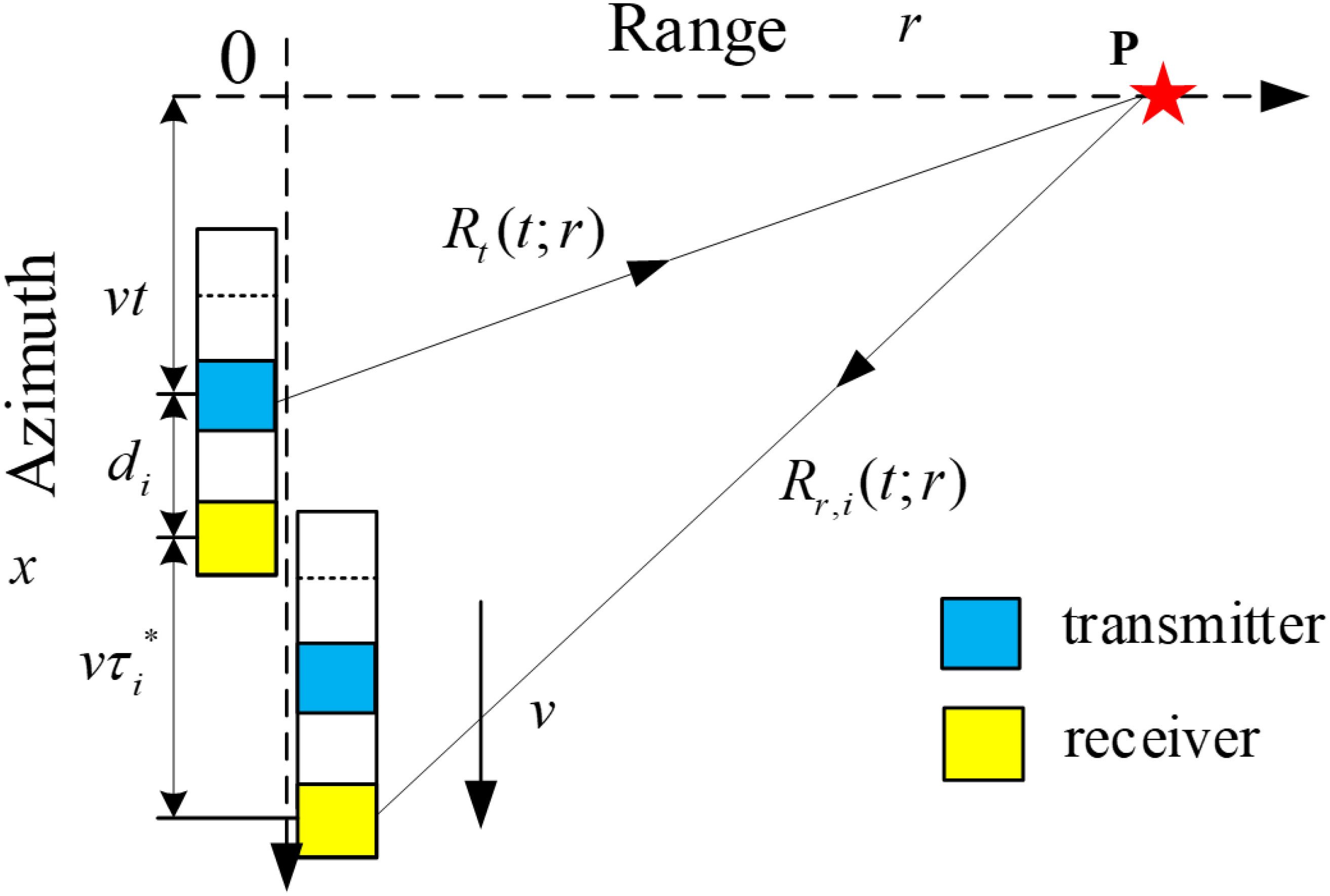
Figure 1 Geometric diagram of multi-receiver SAS.

During the process of moving at v m/s, the transmitter transmits linear frequency modulation (LFM) signal at a fixed pulse repetition frequency (PRF) in orthogonal mode simultaneously. At time $t$, for the point target $P(r,0)$, according to the geometric relationship, the path from the transmitter to the $i\text{th}$ receiver scattered by the point target $P(r,0)$ can be expressed as follows:

$\begin{array}{ll}{R}_i^{*}(t;r)=R_t(t;r)+R_{r,i}(t;r)=\sqrt{r^2+{(vt)}^2}+\sqrt{r^2+{(vt+d_i+v{\tau }_i^{*}(t;r))}^2}& (1)\end{array}$

where, ${\tau }_i^{*}(t;r)$ is the time interval between signal transmission and reception, so the propagation path of sound waves can be written as:

$\begin{array}{ll}{R}_i^{*}(t;r)=c·{\tau }_i^{*}(t;r)& (2)\end{array}$

The exact expression of ${\tau }_i^{*}(t;r)$ can be obtained by combining (1) and (2), and ${\tau }_i^{*}(t;r)$ can be expressed as

$\begin{array}{ll}{\tau }_i^{*}(t;r)=\frac{1}{c^2-v^2}·\{v(vt+d_i)+c\sqrt{{(vt)}^2+r^2}+\sqrt{{\left[v(vt+d_i)+c\sqrt{{(vt)}^2+r^2}\right]}^2+(c^2-v^2){\displaystyle \left[2(vt)d_i+d_i{}^2\right]}}\}& (3)\end{array}$

2.2 Error analysis of AMDSR

Under the narrow-beam assumption, it is generally approximated ${\tau }_i^{*}$ as a range variance $2r/c$, resulting in the error of AMDSR is

$\begin{array}{ll}\Delta x=({\tau }_i^{*}-2r/c)v& (4)\end{array}$

According to the system parameters shown in Table 1, different receivers have different baseline lengths relative to the transmitter.

TABLE 1

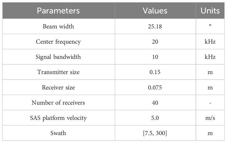
Table 1 MADOM SAS simulation parameters.

We analyzed the receiver with the maximum baseline length and calculated $\Delta x$ across the whole swath under different beam widths. The results are shown in Figure 2.

FIGURE 2

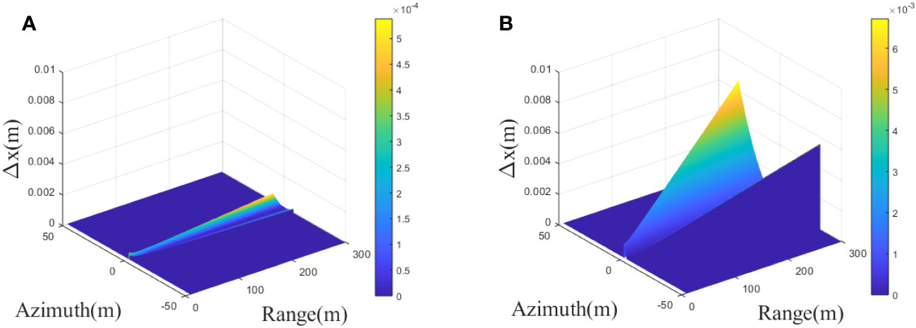
Figure 2 Approximation Error of AMDSR (A) narrow-beam (B) wide-beam.

As shown in Figure 2, $\Delta x$ is maximum at the edge of the beam and increases with range and beam width. The maximum value of narrow-beam SAS is shown in. Figure 2A is 0.0009m, far less than half the length of a receiver (0.025m); the maximum value of wide-beam SAS shown in Figure 2B is 0.007m, which can be compared with the half-length of receiver, which may lead to the problem of azimuth non-uniform sampling. Therefore, under the condition of wide-beam, ${\tau }_i^{*}$ cannot be approximated to $2r/c$, and the azimuth variance must be considered, which means that the range history $R_i^{*}(t;r)$ must adopt a more accurate form.

2.3 Point target echo response model

The accurate range history has a complex form and cannot obtain an analytical expression for the PTRS. The current wide beam algorithms generally use the MSR (Neo et al., 2007; Wu et al., 2016; Zhang et al., 2021), which approximates the accurate range history using Taylor expansion. For example, reference (Zhang et al., 2014) preserves the fourth order term of Taylor expansion, as follows

$\begin{array}{ll}{R}_i(t;r)=k_{0,i}+k_{1,i}t+k_{2,i}{t}^2+k_{3,i}{t}^3+k_{4,i}{t}^4& (5)\end{array}$

where,

$\begin{array}{ll}{k}_{n,i}={\frac{1}{n!}\frac{{\text{d}}^n{R}_i^{\ast }(t;r)}{\text{d}{t}^n}\text{|}}_{t=0}(n=0,1,2,3,4)& (6)\end{array}$

The range history error obtained using the parameters shown in Table 1 is shown in Figure 3, ϵ is range error, λ is the wavelength of signal.

FIGURE 3

Figure 3 Range history error after retaining 4 terms.

It can be seen that under the beam width shown in Table 1, the four-order expansions of the range history can no longer meet the requirement that the maximum range history error is less than (1/16)λ, and the phase error caused cannot be ignored. Meanwhile, preserving different expansion terms has different range history error. In theory, the higher the expansion terms, the more accurate the range history, and the smaller the range history error. We plot the curve of the maximum range history error within the whole beam as a function of the number of Taylor expansions, as shown in Figure 4. It can be seen that the range history error does not decrease indefinitely with the number of expansions. The reason why the error cannot be infinitely reduced is that (Zhang et al., 2014) used narrow beam approximation. When the expansion reaches 10, the range history error is 0.216λ, which is still greater than (1/16)λ. Therefore, this research uses the LIT to derive the PTRS using the original range history, which does not make any approximation to the range history.

FIGURE 4

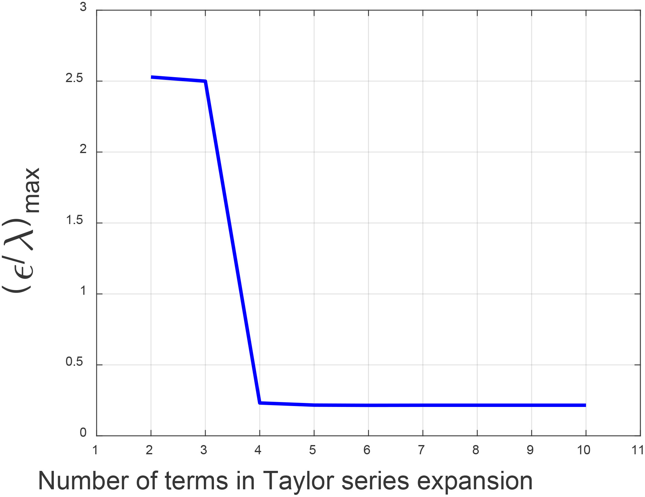
Figure 4 Maximum range history error vs the number of terms.

Let $f_0$ be the carrier frequency of the transmitting signal; $K_r$ is the frequency modulation slope of the transmitted signal; $w_r(·)$ is the envelope of the transmitted signal; $w_a(·)$ is the analytical expression for the antenna pattern; $A_0$ is the signal’s amplitude, it is independent with the imaging quality, so we ignore it in the next context. After demodulation, the baseband form of the $i\text{th}$ echo signal can be expressed as

$\begin{array}{ll}s{s}_i(\tau ,t;r)=A_0·w_r\left(\tau -\frac{R_i(t;r)}{c}\right)·w_a(t)·\exp \left(-j\frac{2\pi f_0{R}_i(t;r)}{c}\right)·\exp \left(j\pi K_r{\left(\tau -\frac{R_i(t;r)}{c}\right)}^2\right)& (7)\end{array}$

To obtain each receiver’s PTRS, the Principle of Stationary Phase (PSP) is performed to simplify range FFT on the baseband signal, and the range spectrum signal is obtained:

$\begin{array}{ll}S{s}_i(f_r,t;r)=A_0{A}_1{W}_r(f_r)w_a(t)\exp \left(-j\frac{2\pi (f_0+f_r)R_i(t;r)}{c}\right)\exp \left(-j\pi {\frac{f_r}{K_r}}^2\right)& (8)\end{array}$

where, $W_r(f_r)=w_r(\frac{f_r}{K_r})$, and $W_{\text{r}}(·)$ is the range frequency envelope, then perform azimuth FFT on (8) to obtain

$\begin{array}{ll}S{S}_i(f_r,f_a;r)={\displaystyle \underset{-\infty }{\overset{+\infty }{\int }}S{s}_i(f_r,t;r)}\exp (-j2\pi f_{a}t)dt& (9)\end{array}$

According to PSP, if the derivative of the phase in the integral expression with respect to $t$ is 0 and the phase stationary time is assumed to be $\tilde{t}$, the following equation can be obtained

$\begin{array}{ll}{f}_a=-\frac{(f_0+f_r)}{c}·\frac{d{R}_i(\tilde{t};r)}{dt}& (10)\end{array}$

From (10), it can be seen that $f_a$ is a function of $\tilde{t}$. According to the LIT (Zhang et al., 2017), if $f_a$ is close-form at a certain value ${\tilde{t}}_0$ and $f_a({\tilde{t}}_0)\ne 0$, which is different from the approximation of $R_i(\tilde{t};r)$in MSR, we can directly obtain the close-form solution of $\tilde{t}$.

$\begin{array}{ll}\tilde{t}={\displaystyle \sum _{n=1}^3\underset{\tilde{t}\to 0}{\lim }\frac{{[f_a(\tilde{t})-f_a(0)]}^n}{n!}\frac{d^{n-1}}{d{t}^{n-1}}{\left[\frac{\tilde{t}-0}{f_a(\tilde{t})-f_a(0)}\right]}^n}& (11)\end{array}$

Take ${\tilde{t}}_0=0$ and $n=3$, and bring (10) into (11), then there is

$\begin{array}{ll}{\tilde{t}}_i=-\frac{1}{R_i^{(2)}(0;r)}\left(\frac{f_a-f_a(0)}{f_0+f_r}c\right)-\frac{R_i^{(3)}(0;r)}{2{(R_i^{(2)}(0;r))}^3}{\left(\frac{f_a-f_a(0)}{f_0+f_r}c\right)}^2+\left(\frac{1}{6}\frac{R_i^{(4)}(0;r)}{{(R_i^{(2)}(0;r))}^4}-\frac{1}{2}\frac{{(R_i^{(3)}(0;r))}^2}{{(R_i^{(2)}(0;r))}^5}\right){\left(\frac{f_a-f_a(0)}{f_0+f_r}c\right)}^3& (12)\end{array}$

The PTRS of the $i\text{th}$ receiver is obtained by integrating (12) into the phase of (9), and we can get

$\begin{array}{ll}S{S}_i(f_r,f_a;r)=A·W_r(f_r)·W_a(f_a)·\exp (j{\phi }_i(f_r,f_a;r))& (13)\end{array}$

where,

$\begin{array}{ll}{\phi }_i(f_r,f_a;r)=-\frac{2\pi (f_0+f_r)R_i({\tilde{t}}_i;r)}{c}-\pi {\frac{f_r}{K_r}}^2-2\pi f_a{\tilde{t}}_i& (14)\end{array}$

In order to analyze the phase errors between the PTRS obtained by different methods and the accurate PTRS, we selected the receiver 40 as the analysis object according to the parameters of the wide-beam SAS system shown in Table 1. We obtained the PTRS’s phase errors of the MSR and LIT at 3 point targets at different ranges, as shown in Figures 5, 6A–C. represent the phase errors of point targets at ranges of 50m, 150m, and 250m, respectively. Comparing Figures 5, 6, it can be seen that the phase error increases with the range and the azimuth frequency. However, the phase error of the LIT is always significantly smaller than MSR. The maximum value of phase error of LIT in $(0m,250m)$ is 0.019rad, which is much smaller than $\pi /4$ (Ning et al., 2023). Therefore, under the wide-beam SAS system parameter, the method proposed in this paper can meet the requirements of high-resolution imaging across the whole swath.

FIGURE 5

Figure 5 Phase error of PTRS of MSR at different ranges (A) r=50m (B) r=150 m (C) r=250m.

FIGURE 6

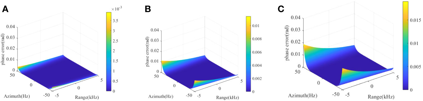
Figure 6 Phase error of PTRS of LIT at different ranges (A) r=50m (B) r=150 m (C) r=250m.

Expanding (14) to a series of $f_r$. To apply the method in this research to the wide beam condition, we reserve the cubic term to obtain:

$\begin{array}{ll}{\phi }_i(f_a,f_r;r)={\phi }_{az,i}(f_a;r)+{\phi }_{rcmc,i}(f_a;r)f_r+{\phi }_{rc}{f}_r^2+{\phi }_{src,i}(f_a;r)f_r^2+{\phi }_{cubic,i}(f_a;r)f_r^3& (15)\end{array}$

where, ${\phi }_{az,i}(f_a;r)$ is the azimuth modulation term; ${\phi }_{rcmc,i}(f_a;r)$ is the range migration term; ${\phi }_{rc}$ is the range frequency modulation term; ${\phi }_{src,i}(f_a;r)$ is the second range compression term; ${\phi }_{cubic,i}(f_a;r)$ is the third-order coupling term of range and azimuth. According to the definitions of $R_{rd,i}(f_a;r)$ and $K{m}_i(f_a;r)$, we can get

$\begin{array}{ll}{R}_{rd,i}(f_a;r)=\frac{{\phi }_{rcmc,i}(f_a;r)}{-2\pi }·c& (16)\end{array}$

$\begin{array}{ll}K{m}_i(f_a;r)=\frac{\pi }{{\phi }_{src,i}(f_a;r)+{\phi }_{rc}}& (17)\end{array}$

$R_{rd,i}(f_a;r)$ is the range migration curve of the $i\text{th}$ receiver in the range-Doppler domain; $K{m}_i(f_a;r)$ is the equivalent frequency modulation slope of the range compression filter for the $i\text{th}$ receiver. Bring (16) and (17) into (15), $S{S}_i(f_{\text{r}},f_a;r)$ can be rewritten as

$\begin{array}{ll}S{S}_i(f_{\text{r}},f_a;r)=W_r(f_r)W_a(f_a)\exp (+j{\phi }_{az,i}(f_a;r))\text{exp}\left(-j\frac{2\pi R_{rd,i}(f_a;r)}{c}{f}_r\right)\text{exp}\left(+j\frac{\pi }{K{m}_i(f_a;r)}{f}_r^2\right)\text{exp}\left(+j{\phi }_{cubic,i}(f_a;r)f_r^3\right)& (18)\end{array}$

The different receiver has different coefficients such as $R_{rd,i}$ and $K{m}_i$, which means that for the same point target, the different receiver has different point target echo responses. Therefore, it is necessary to perform matching filtering processing separately for each receiver.

3 Imaging algorithm derivation

The flowchart of the imaging algorithm is shown in Figure 7, where FFT represents the Fast Fourier Transform; IFFT is Inverse Fast Fourier Transform. The algorithm includes six-fold FFT/IFFT, one-fold azimuth spectrum extension, six-fold phase multiplication, and one-fold azimuth spectrum superposition. The azimuth spectrum extension is used to increase the length of one receiver’s data to meet the requirements of signal processing, but the processed signal is highly under-sampled in the azimuth frequency, which can cause azimuth spectrum aliasing. The azimuth spectrum coherent superposition is used to suppress the azimuth spectrum aliasing caused by azimuth under-sampling.

FIGURE 7

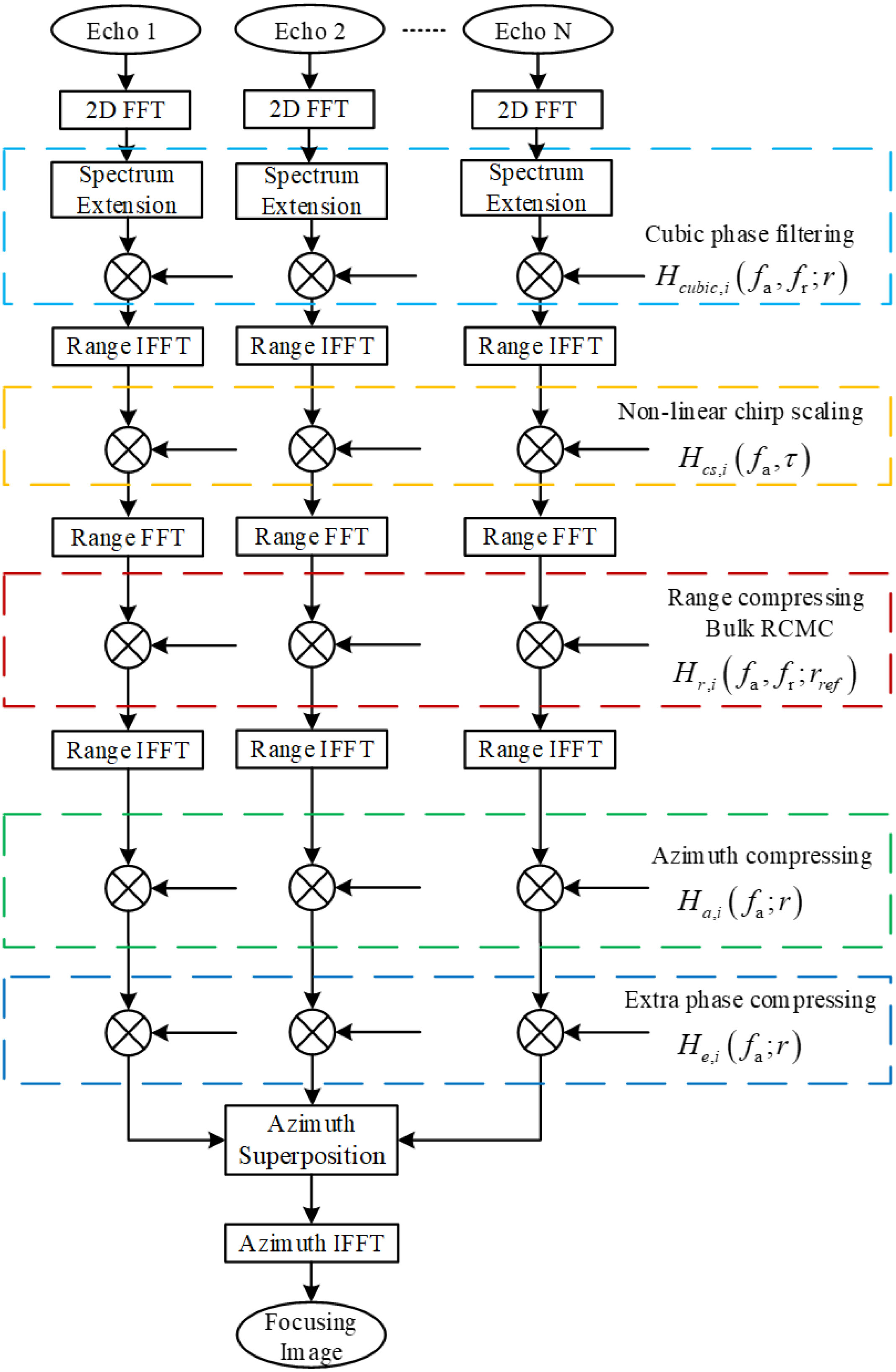
Figure 7 Algorithm flowchart.

3.1 Approximation of equivalent frequency modulation slope

Compared to traditional RDA and CSA, this paper considers the linear relationship of $K{m}_i$ with $r$ and approximates $K{m}_i$ at the reference range

$\begin{array}{ll}K{m}_i(f_a;r)=K{m}_{i,r_{ref}}+K{s}_{i,r_{ref}}·(r-r_{ref})& (19)\end{array}$

where $K{s}_{i,r_{ref}}$ is the first derivative of $K{m}_i(f_a;r)$ at $r_{ref}$, expressed as

$\begin{array}{ll}K{s}_{i,r_{ref}}=-\pi ·\frac{{{\phi }^{\prime }}_{src,i}(f_a;r_{ref})}{{({\phi }_{src,i}(f_a;r_{ref})+{\phi }_{rc})}^2}& (20)\end{array}$

where, $r_{ref}$ generally takes the center position of the whole swath.

3.2 Cubic phase filtering

In order to eliminate the influence of the cubic term of $f_r$, a cubic phase filter is performed on $S{S}_i(f_{\text{a}},f_{\text{r}};r)$ in the 2D frequency domain. The expression of the cubic phase filter is

$\begin{array}{ll}{H}_{cubic,}{}_i(f_r,f_a;r)=\exp (j2\pi Y_i(f_a)f_r^3/3)& (21)\end{array}$

where, $Y_i(f_a)$ is the coefficient of the cubic phase filter that varies with the azimuth frequency $f_a$, with the aim of filtering out the cubic phase of the range frequency $f_r$ and the cubic phase error generated by subsequent nonlinear Chirp Scaling. Since ${\phi }_{cubic,i}(f_a;r)$ is weakly dependent on the range (Neo et al., 2008), ${\phi }_{cubic,i}(f_a;r_{ref})$ can substitute ${\phi }_{cubic,i}(f_a;r)$, and $Y{m}_i(f_a)$ is the error after the cubic phase filtering

$\begin{array}{ll}{Y}_i(f_a)=Y{m}_i(f_a)-\frac{3}{2\pi }{\phi }_{cubic,i}(f_a;r_{ref})& (22)\end{array}$

The obtained PTRS after cubic phase filtering on (7) is

$\begin{array}{ll}\begin{array}{l}S{S}_{c,i}(f_r,f_a;r)=S{S}_i(f_r,f_a;r)·H_{cubic,}{}_i(f_r,f_a;r)\\ =W_{\text{r}}(f_r)W_a(f_a)\times \exp (j{\phi }_{az,i}(f_a;r))\times \exp \left(-j\frac{2\pi R_{rd,i}(f_a;r)}{c}{f}_r\right)\times \exp \left(j\frac{\pi }{K{m}_i(f_a;r)}{f}_r^2\right)\times \exp \left(j\frac{2\pi Y{m}_i{f}_r^3}{3}\right)\end{array}& (23)\end{array}$

3.3 Non-linear chirp scaling

Using PSP for range IFFT, the signal obtained in the range-Doppler domain is

$\begin{array}{ll}s{S}_i(\tau ,f_a;r)={\omega }_r\left(\frac{K{m}_i}{K_r}\left(\tau -\frac{2r}{c{\gamma }_i}\right)\right)W_a(f_a)\exp (+j{\phi }_{az,i}(f_a;r))\exp (-j\pi K{m}_i{(\tau -{\tau }_d)}^2)\exp \left(-j\frac{2\pi Y{m}_{i}K{m}_i^3{(\tau -{\tau }_d)}^3}{3}\right)& (24)\end{array}$

where ${\gamma }_i=\frac{2}{R_{rd,i}^{\text{'}}(f_a;r_{ref})}$.

Let the expression of the non-linear chirp scaling equation be

$\begin{array}{ll}{H}_{cs,i}(\tau ,f_a)=\exp (-j\pi q_{2,i}{(\tau -{\tau }_{ref})}^2)·\exp \left(-j\frac{2\pi q_{3,i}{(\tau -{\tau }_{ref})}^3}{3}\right)& (25)\end{array}$

where, $q_{2,i}$ and $q_{3,i}$ are undetermined coefficients, which will be solved later in the text.

Perform non-linear Chirp Scaling on $s{S}_i(\tau ,f_a;r)$ to obtain

$\begin{array}{ll}s{S}_{cs,i}(\tau ,f_a;r)=s{S}_i(\tau ,f_a;r)\times H_{cs,i}(\tau ,f_a)& (26)\end{array}$

To obtain the coefficients of the cubic phase filter and the scaling equation, the range IFFT of $s{S}_{cs,i}(\tau ,f_a;r)$ is performed to the 2D frequency domain, and then the series expansion of $f_r$ is performed, retaining the cubic term. After the above operation, we can obtain

$\begin{array}{ll}\begin{array}{c}S{S}_{cs,i}(f_r{f}_a{;}_r)=W_r(f_r)·W_a(f_a)\exp \left(j\frac{2\pi (K{m}_i^{3}Y{m}_i+q_{3,i})f_r^3}{3{(K{m}_i+q_{2,i})}^3}\right)\exp \left(j\frac{\pi }{K{m}_i+q_{2,i}}{f}_r^2\right)\exp \left(j\frac{2\pi K{m}_i({\tau }_d-{\tau }_{ref})(K{m}_i^{2}Y{m}_i{q}_{2,i}-q_{3,i})}{K{m}_i+q_{2,i}{)}^3}{f}_r^2\right)\\ \exp \left(j-\frac{2\pi ({\tau }_{d}K{m}_i+q_{2,i}{\tau }_{ref})}{K{m}_i+q_{2,i}}{f}_r\right)\exp \left(j\frac{2\pi K{m}_i^2{({\tau }_d-{\tau }_{ref})}^2(K{m}_{i}Y{m}_i{q}_{2,i}^2+q_{3,i})}{{(K{m}_i+q_{2,i})}^3}{f}_r\right)\exp (j{\phi }_{az,i}(f_a;r))exp\left(-j\frac{\pi K{m}_i{q}_{2,i}{({\tau }_d-{\tau }_{ref})}^2}{K{m}_i+q_{2,i}}\right)\\ \exp \left(j\frac{2\pi K{m}_i^3{({\tau }_d-{\tau }_{ref})}^3(Y{m}_i{q}_{2,i}^3-q_{3,i})}{3{(K{m}_i+q_{2,i})}^3}\right)\end{array}& (27)\end{array}$

After bringing (19) and $\tau =2r/(c{\gamma }_i)$, ${\tau }_{ref}=2r_{ref}/(c{\gamma }_i)$, and $\Delta \tau ={\tau }_d-{\tau }_{ref}$ into (27), and then expanding the coefficients of each order of $f_{\text{r}}$ into the series of $\Delta \tau$, we can obtain the three undetermined coefficients as follows

$\begin{array}{ll}{Y}_{m,i}=\frac{K{s}_i{{}_{,}}_{r_{ref}}(2{\alpha }_i-1)}{2K{m}_i^3{}_{r_{ref}}({\alpha }_i-1)}& (28)\end{array}$

$\begin{array}{ll}{q}_{2,i}=K{m}_{i,}{}_{r_{ref}}({\alpha }_i-1)& (29)\end{array}$

$\begin{array}{ll}{q}_{3,i}=\frac{({\alpha }_i-1)K{s}_{i,r_{ref}}}{2}& (30)\end{array}$

where ${\alpha }_i=\frac{{\gamma }_i(f_{ac})}{{\gamma }_i(f_a)}$, the phase expression of the scaled signal obtained by bringing (28), (29) and (30) into (27) is

$\begin{array}{ll}\begin{array}{c}{\varphi }_{cs,i}(f_r{f}_a;r)=\frac{\pi f_r^2}{K{m}_{i,r_{ref}}{\alpha }_i}+\frac{f_r^{3}K{s}_{i,r_{ref}}\pi }{3{\alpha }_i({\alpha }_i-1)K{m}_{i,ref}^3}+\left(\left(-\frac{4\pi }{{\gamma }_{i}c}+\frac{4\pi }{c{\gamma }_i{\alpha }_i}\right)r_{ref}-\frac{4\pi r}{c{\gamma }_i{\alpha }_i}\right)f_r+{\phi }_{az,i}(f_a;r)\\ -\frac{\pi K{m}_{i,r_{ref}}({\alpha }_i-1)\Delta {\tau }^2}{{\alpha }_i}-\frac{({\alpha }_i-1)K{s}_{i,r_{ref}}\pi \Delta {\tau }^3}{3{\alpha }_i}\end{array}& (31)\end{array}$

3.4 Range processing

By compensating for the first, second, and bulk RCMC terms in a phase multiplication, and simultaneously completing bulk RCMC, range compression, and cubic coupling term compensation, the phase multiplication factor is

$\begin{array}{ll}{H}_{r,i}(f_a,f_r;r_{ref})=\exp \left(j\left(\frac{4\pi }{{\gamma }_{i}c}-\frac{4\pi }{c{\gamma }_i{\alpha }_i}\right)r_{ref}{f}_r\right)\exp \left(j\frac{\pi }{K{m}_{i,ref}{\alpha }_i}{f}_r^2\right)\exp \left(j\frac{K{s}_{i,ref}\pi }{3{\alpha }_i({\alpha }_i-1)K{m}_{i,ref}^3}{f}_r^3\right)& (32)\end{array}$

Perform range IFFT, and the obtained the phase of signal in range-Doppler domain is

$\begin{array}{ll}s{S}_{rc,i}(f_a;r)=p_r\left(\tau -\frac{2r}{c{\gamma }_i{a}_i}\right).W_a(f_a)\exp (j{\phi }_{az,i}(f_a;r))exp\left(-j\frac{(a_i-1)k{s}_{i,ref}\pi \Delta {\tau }^3}{3a_i}\right)\exp \left(-j\frac{\pi K{m}_{i,ref}(a_i-1)\Delta {\tau }^2}{a_i}\right)& (33)\end{array}$

where $p_r(·)$ is the Sinc function.

3.5 Azimuth processing

The azimuth compressing term $H_{a,i}(f_a;r)$ and the extra phase compensation factor $H_{e,i}(f_a;r)$ are respectively

$\begin{array}{ll}{H}_{a,i}(f_a;r)=\exp \left(-j\left({\phi }_{az,i}\left(f_a;r\right)\right)\right)& (34)\end{array}$

$\begin{array}{ll}{H}_{e,i}(f_a;r)=exp\left(j\frac{\pi (a_i-1)K{m}_{i,r_{ref}}\Delta {\tau }^2}{a_i}\right)\exp \left(+j\frac{\pi (a_i-1)K{s}_{i,r_{ref}}\Delta {\tau }^3}{3a_i}\right)& (35)\end{array}$

After compensation, coherent superposition in the azimuth frequency domain is performed on each receiver, and then the azimuth IFFT is performed to obtain the focused SAS image.

4 Algorithm validation

4.1 Simulation experiment

To verify the effectiveness of the algorithm proposed in this research, simulations were conducted on ideal point targets at different ranges. The positions of 10 ideal point targets are shown in Figure 8, where $P_1\sim P_5$ are close-range targets and $P_6\sim P_{10}$ are long-range targets. Computer CPU is Intel i7-10700@2.90G, RAM is 32 GB, Matlab version R2020a.

FIGURE 8

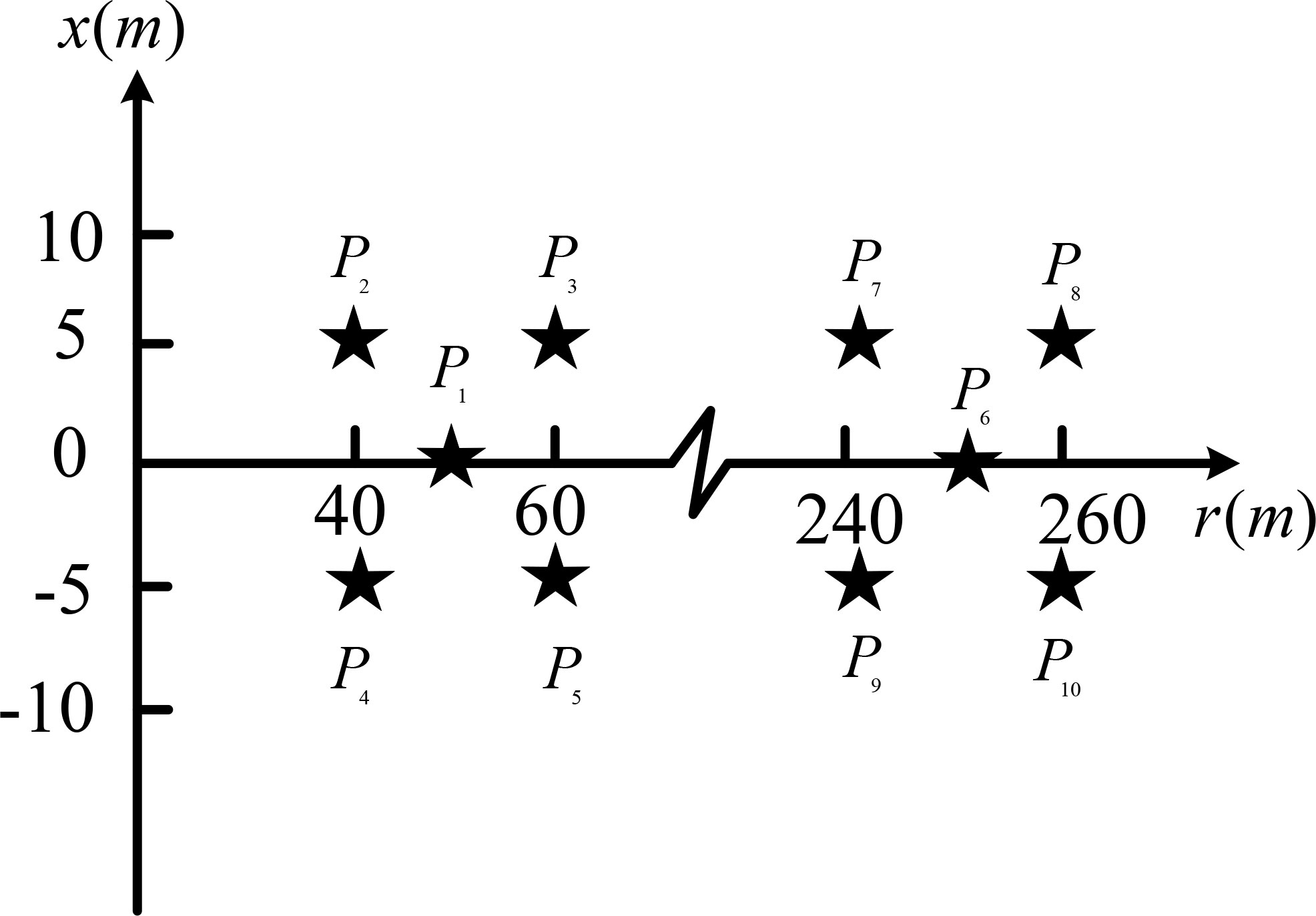
Figure 8 Simulation point targets setting.

In the simulation experiment, it is assumed that the distribution of the transmitter and receiver is shown in Figure 1, and the parameters are shown in Table 1. The wide-beam imaging algorithms proposed in the RDA-MSR (Zhang et al., 2014), the RDA-MRCMC (Zhang, 2014), and this research were used to image point targets shown in Figure 8. The imaging results obtained are shown in Figure 9, where Figures 9A, B are the results of the RDA-MSR; Figures 9C, D are the results of the RDA-MRCMC; Figures 9E, F are the results of the proposed method in this research. It can be seen that the RDA-MRCMC has the worst imaging performance. This is because transforming the multi-receiver SAS into a mono-static SAS model, although the imaging process was simplified, there were significant errors.

FIGURE 9

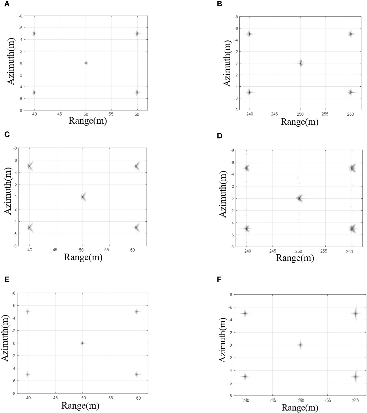
Figure 9 Imaging results of different methods (A) P₁ ~ P₅ (RDA-MSR) (B) P₆ ~ P₁₀ (RDA-MSR) (C) P₁ ~ P₅ (RDA-MRCMC) (D) P₆ ~ P₁₀ (the RDA-MRCMC) (E) P₁ ~ P₅ (the proposed method) (F) P₆ ~ P₁₀ (the proposed method).

To quantitatively compare the effectiveness of different methods, we take the range and azimuth slices of point targets P₁ and P₆ as shown in Figures 10, 11, respectively, with amplitude units in dB.

FIGURE 10

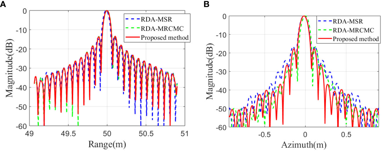
Figure 10 Slices of P₁ (A) Range slice (B) Azimuth slice.

FIGURE 11

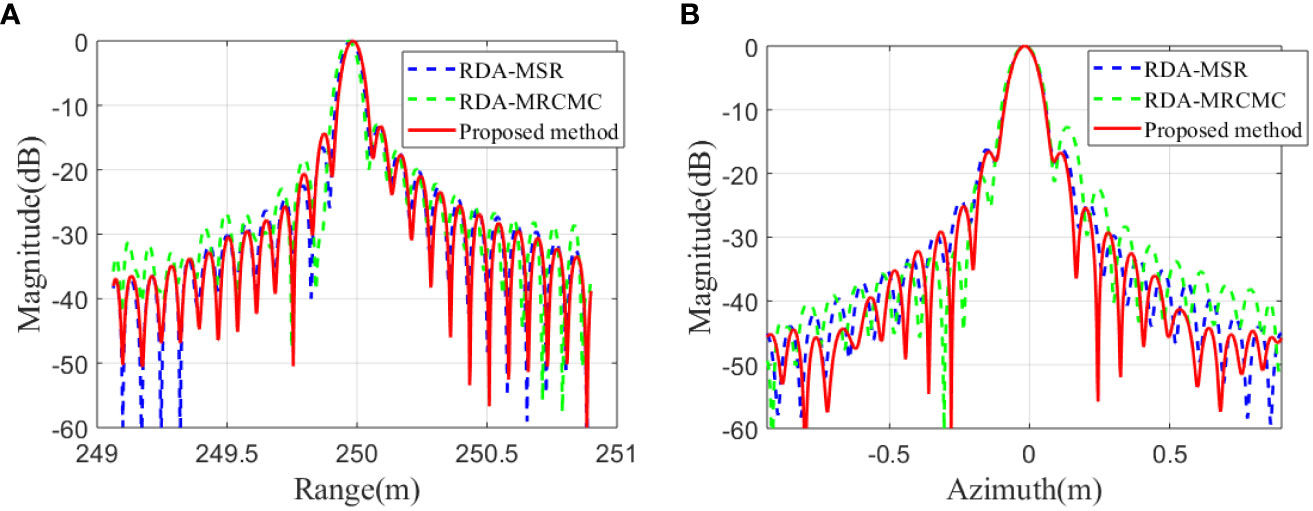
Figure 11 Slices of P₆ (A) Range slice (B) Azimuth slice.

The blue dashed line represents the RDA-MSR, the green dashed line represents the RDA-MRCMC, and the red solid line represents the method in this research. The impulse response width (IRW), peak side lobe ratio (PSLR), and integral side lobe ratio (ISLR) of the range slice and azimuth slice were measured, and the results are shown in Table 2.

TABLE 2

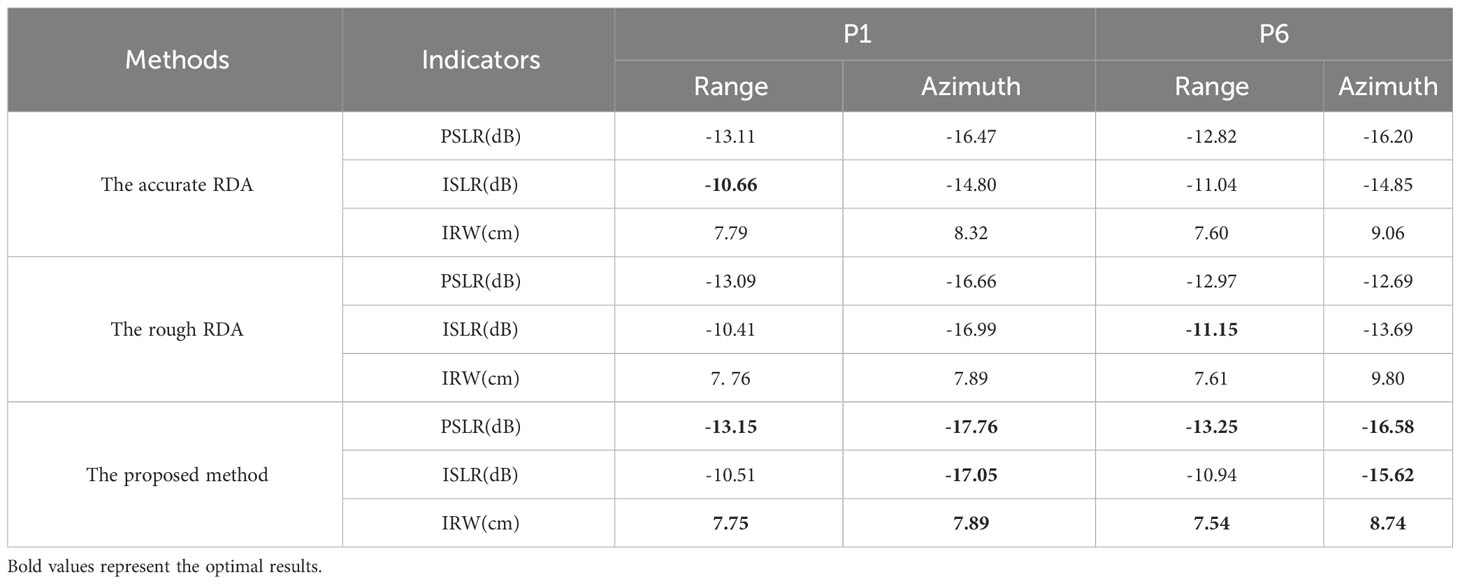
Table 2 Quality parameters of different methods.

From Table 2, it can be seen that the imaging effect of the proposed method is similar to that of the RDA-MSR, but the interpolation operation in this method is not efficient enough. We calculated the time required for imaging the point target echo signal in the scene shown in Figure 8, as shown in Table 3, our method avoids interpolation and saves about half of the time of the RDA-MSR and demonstrates the advantages of computation cost.

TABLE 3

Table 3 Time cost of different methods under simulation.

4.2 Field test

To further validate the effectiveness of our method, imaging was performed on the data obtained from a sea trial of ChinSAS in 2017 (Zhang et al., 2012). The parameters of ChinSAS-150 are as follows: carrier frequency is 75kHz, transmitter’s length is 0.16m, receiver’s length is 0.08m, the signal bandwidth is 20kHz, the total number of receivers participating in imaging is 37, SAS platform speed is 2.5m/s, and size of imaging block is 40m(azimuth)×50m(range). Based on the comprehensive analysis of the above parameters, the system operates in a narrow-beam scenario. Comparing Figures 12A–C, it is not difficult to find that the imaging results of all methods are almost identical, but the proposed method is faster than the RDA-MSR. This demonstrates the effectiveness of our method in practical applications. Due to the lack of publicly available field data on wide-beam multi-receiver SAS in China, the advantages of this method in wide-beam imaging still need further verification. We will next carry out the development of low-frequency wide-beam SAS and verify its practicality with the method proposed in this research as soon as possible.

FIGURE 12

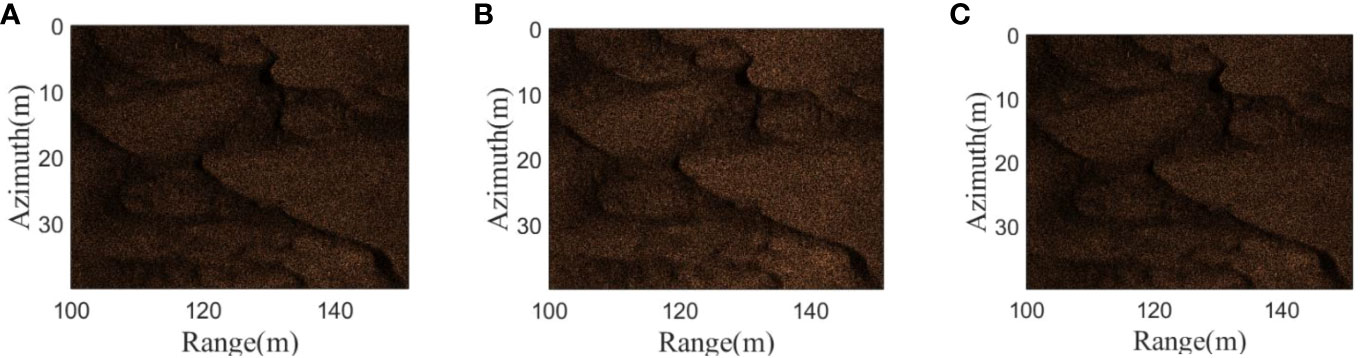
Figure 12 Comparison of results from different methods when processing field data (A) the RDA-MSR (B) the RDA-MRCMC (C) the proposed method.

We recorded the operation time of the field data imaging under different methods, as shown in Table 4. It can be seen from the Table 4 that the proposed method takes two-thirds of the time required for RDA-MSR. Although the proposed method takes longer than RDA-MRCMC, this method will have better focusing result under wide beam conditions, so it is a compromise between computation load and imaging quality.

TABLE 4

Table 4 Time cost of different methods under field data.

5 Conclusion

This research proposes a NCSA for multi-receiver SAS based on azimuth spectrum superposition, which adopts the more accurate PTRS based on LIT and the NCS algorithm to solve the problem of poor imaging quality of existing wide-beam multi-receiver SAS. The algorithm provided in this study provides theoretical support for the future development of low-frequency wide-beam SAS.

Data availability statement

The code used in this study has been deposited in a publicly accessible repository, which can be found here: https://gitee.com/freepoet/ncsa.

Author contributions

MN wrote the program and the original manuscript. HZ provided fundings and field test data to support this research. HL translated and polished this paper. MM and LD provided valuable insights for this research and result analysis. JT proposed this problem and the methodology. All authors contributed to this paper and approved the submitted manuscript.

Funding

This research was supported in part by the National Natural Science Foundation of China under Grant 42176187 and Grant 62301592.

Acknowledgments

Special thanks to the fundings that provided support for this research.

Conflict of interest

The authors declare that the research was conducted in the absence of any commercial or financial relationships that could be construed as a potential conflict of interest.

Publisher’s note

All claims expressed in this article are solely those of the authors and do not necessarily represent those of their affiliated organizations, or those of the publisher, the editors and the reviewers. Any product that may be evaluated in this article, or claim that may be made by its manufacturer, is not guaranteed or endorsed by the publisher.

References

Bellettini A., Pinto M. A. (2002). Theoretical accuracy of synthetic aperture sonar micronavigation using a displaced phase-center antenna. IEEE J. Oceanic Eng. 27 (4), 780–789. doi: 10.1109/JOE.2002.805096

CrossRef Full Text | Google Scholar

Bonifant W. W. (1999). Interferometic synthetic aperture sonar processing (Atlanta, Georgia: George Institute of Technology). Master.

Google Scholar

Callow H. J. (2003). Signal Processing for Synthetic Aperture Sonar Image Enhancement (Christchurch, New Zealand: Electrical and Electronic Engineering, University of Canterbury). Ph.D.

Google Scholar

Duan J., Huang Y., Liu J. (2017). Application of FFBP algorithm to SAS imaging in non-linear trajectory with non-uniform speeds. J. Appl. Acoustics 36 (1), 6.

Google Scholar

Giardina P. E. (2012). Interferometric Synthetic Aperture Sonar Signal Processing for Autonomous Underwater Vehicles Operating in Shallow Water (New Orleans, Louisiana: University of New Orleans).

Google Scholar

Gough P., Hayes M., Wilkinson D. (2004). An efficient image reconstruction algorithm for a multiple hydrophone array synthetic aperture sonar.

Google Scholar

Huang P., Yang P. (2022). Synthetic aperture imagery for high-resolution imaging sonar. Front. Mar. Sci. 9. doi: 10.3389/fmars.2022.1049761

PubMed Abstract | CrossRef Full Text | Google Scholar

Jiang X., Sun C., Feng J. (2004). “A novel image reconstruction algorithm for synthetic aperture sonar with single transmitter and multiple-receiver configuration,” in Oceans '04 MTS/IEEE Techno-Ocean '04, 9–12. Kobe, Japan: IEEE. Cat. No.04CH37600.

Google Scholar

Li C., Zhang H., Deng Y. (2021). Focus improvement of airborne high-Squint bistatic SAR data using modified azimuth NLCS algorithm based on lagrange inversion theorem. Remote Sens. 13 (10), 19165. doi: 10.3390/rs13101916

CrossRef Full Text | Google Scholar

Li Y., Zhang T., Mei H., Quan Y., Xing M. (2022). Focusing translational-variant bistatic forward- looking SAR data using the modified omega-K algorithm. IEEE Trans. Geosci. Remote Sens. 60, 1–16. doi: 10.1109/TGRS.2021.3063780

CrossRef Full Text | Google Scholar

Liao Y., Liu Q. H. (2017). Modified chirp scaling algorithm for circular trace scanning synthetic aperture radar. IEEE Trans. Geosci. Remote Sens. 55 (12), 7081–7091. doi: 10.1109/TGRS.2017.2740063

CrossRef Full Text | Google Scholar

Liu W., Zhang C., Liu J. (2009). Application of FFBP algorithm to synthetic aperture sonar imaging. Tech. Acoustics 28 (5), 572–576.

Google Scholar

Ma M., Tang J., Wu H., Zhang P., Ning M. (2023). CZT algorithm for the doppler scale signal model of multireceiver SAS based on shear theorem. IEEE Trans. Geosci. Remote Sens. 61, 1–12. doi: 10.1109/TGRS.2023.3234572

CrossRef Full Text | Google Scholar

Ma M., Tang J., Zhong H. (2020). CZT algorithm for multiple-receiver synthetic aperture sonar. IEEE Access 8, 1902–1909. doi: 10.1109/ACCESS.2019.2962314

CrossRef Full Text | Google Scholar

Marx D., Nelson M., Chang E., Gillespie W., Putney A., Warman K. (2000). “An introduction to synthetic aperture sonar,” in Proceedings of the Tenth IEEE Workshop on Statistical Signal and Array Processing (Cat. No.00TH8496), Pittsburgh, PA, USA: IEEE. 16–16.

Google Scholar

Neo Y. L., Wong F., Cumming I. G. (2007). A two-dimensional spectrum for bistatic SAR processing using series reversion. IEEE Geosci. Remote Sens. Lett. 4 (1), 93–96. doi: 10.1109/LGRS.2006.885862

CrossRef Full Text | Google Scholar

Neo Y. L., Wong F. H., Cumming I. G. (2008). Processing of azimuth-invariant bistatic SAR data using the range doppler algorithm. IEEE Trans. Geosci. Remote Sens. 46 (1), 14–21. doi: 10.1109/TGRS.2007.909090

CrossRef Full Text | Google Scholar

Ning M., Zhong H., Wu H., Zhang J., Tang J. (2023). “Range doppler algorithm for wide-beam multi-receiver synthetic aperture sonar considering differential range curvature,” in 2023 4th International Conference on Computer Engineering and Application (ICCEA), Hangzhou, China: IEEE, 7-9 April 2023.

Google Scholar

Qian Y., Kuang H., Zhang Y., Zhang Y. (2021). “Modified generalized omega-K algorithm for low earth orbit high resolution spotlight spaceborne SAR focusing,” in 2021 IEEE International Geoscience and Remote Sensing Symposium IGARSS, Brussels, Belgium: IEEE, 11-16 July 2021.

Google Scholar

Raney R. K., Runge H., Bamler R., Cumming I. G., Wong F. H. (1994). Precision SAR processing using chirp scaling. IEEE Trans. Geosci. Remote Sens. 32 (4), 786–799. doi: 10.1109/36.298008

CrossRef Full Text | Google Scholar

Synnes S. A. V., Hunter A. J., Hansen R. E., Sæbø T. O., Callow H. J., van Vossen R., et al. (2017). Wideband synthetic aperture sonar backprojection with maximization of wave number domain support. IEEE J. Oceanic Eng. 42 (4), 880–891. doi: 10.1109/JOE.2016.2614717

CrossRef Full Text | Google Scholar

Tan C., Zhang X., Yang P., Sun M. (2019). A novel sub-bottom profiler and signal processor. Sensors (Basel Switzerland) 19, 5052. doi: 10.3390/s19225052

PubMed Abstract | CrossRef Full Text | Google Scholar

Tian Z., Tang J., Zhong H., Zhang S. (2016). Extended range doppler algorithm for multiple-receiver synthetic aperture sonar based on exact analytical two-dimensional spectrum. IEEE J. Oceanic Eng. 41 (1), 164–174. doi: 10.1109/JOE.2015.2402053

CrossRef Full Text | Google Scholar

Tian Z., Zhong H., Tang J., Zhang J. (2022). Azimuth-invariant motion compensation and imaging chirp scaling algorithm for multiple-receiver synthetic aperture sonar. IEEE Access 10, 114060–114076. doi: 10.1109/ACCESS.2022.3218279

CrossRef Full Text | Google Scholar

Vu V. T., Sjögren T. K., Pettersson M. I. (2014). Two-dimensional spectrum for biSAR derivation based on lagrange inversion theorem. IEEE Geosci. Remote Sens. Lett. 11 (7), 1210–1214. doi: 10.1109/LGRS.2013.2289735

CrossRef Full Text | Google Scholar

Wang R., Loffeld O., Nies H., Knedlik S., Ender J. H. G. (2009). Chirp-scaling algorithm for bistatic SAR data in the constant-offset configuration. IEEE Trans. Geosci. Remote Sens. 47 (3), 952–964. doi: 10.1109/TGRS.2008.2006275

CrossRef Full Text | Google Scholar

Wang X., Zhang X., Zhu S. (2015). “Upsampling based back projection imaging algorithm for multi-receiver synthetic aperture sonar,” in 2015 International Industrial Informatics and Computer Engineering Conference. Xi'an, Shaanxi, China: ATLANTIS PRESS.

Google Scholar

Wilkinson D. R. (2001). Efficient Image Reconstruction Techniques for a Multiple-Receiver Synthetic Aperture Sonar (Christchurch, New Zealand: Electrical and Electronic Engineering, University of Canterbury). Master.

Google Scholar

Wu H., Tang J., Zhong H. (2019). Moderate squint imaging algorithm for the multiple-hydrophone SAS with receiving hydrophone dependence. IET Radar Sonar Navigation 13(1), 139-147. doi: 10.1049/iet-rsn.2018.5055

CrossRef Full Text | Google Scholar

Wu J., Pu W., Huang Y., Yang J., Yang H. (2016). “An Omega-K algorithm for bistatic forward-looking SAR based on spectrum modeling and optimization,” in 2016 CIE International Conference on Radar (RADAR), Guangzhou, China: IEEE, 10-13 Oct. 2016.

Google Scholar

Xiong T., Xing M., Wang Y., Guo R., Sheng J., Bao Z. (2011). Using derivatives of an implicit function to obtain the stationary phase of the two-dimensional spectrum for bistatic SAR imaging. IEEE Geosci. Remote Sens. Lett. 8 (6), 1165–1169. doi: 10.1109/LGRS.2011.2159090

CrossRef Full Text | Google Scholar

Xu J., Tang J., Zhang C. (2003). Multi-aperture synthetic aperture sonar lmaging algorithm. Signal Process. 19 (2), 4. doi: 10.3969/j.issn.1003-0530.2003.02.016

CrossRef Full Text | Google Scholar

Yang P., Liu J. (2022). “Effect of non-unifrom sampling on sonar focusing,” in 2022 14th International Conference on Communication Software and Networks (ICCSN), Chongqing, China: IEEE, 10-12 June 2022.

Google Scholar

Zhang X. (2014). Study on multi-receiver synthetic aperture sonar imagery and motion compensation algorithm. 36 (7).

Google Scholar

Zhang X., Dai X., Yang Bo. (2018). Fast imaging algorithm for the multiple receiver synthetic aperture sonars. IET Radar Sonar Navigation 6, 74303-74319. doi: 10.1049/iet-rsn.2018.5040

CrossRef Full Text | Google Scholar

Zhang X., Huang H., Ying W., Wang H., Xiao J. (2017). An indirect range-Doppler algorithm for multireceiver synthetic aperture sonar based on lagrange inversion theorem. IEEE Trans. Geosci. Remote Sens. 55 (6), 3572–35875. doi: 10.1109/TGRS.2017.2676339

CrossRef Full Text | Google Scholar

Zhang T., Li Y., Song X., Zhang T., Wu C., Sun Z. (2021). “A modified omega-K algorithm for bistatic forward-looking SAR data imaging,” in 2021 CIE International Conference on Radar (Radar), Haikou, Hainan: IEEE, 15-19 Dec. 2021.

Google Scholar

Zhang S., Sheng J., Xing M. (2018). A novel focus approach for squint mode multi-channel in azimuth high-resolution and wide-swath SAR imaging processing. IEEE Access 6, 74303–74319. doi: 10.1109/ACCESS.2018.2873739

CrossRef Full Text | Google Scholar

Zhang X., Tan C. (2018). “A comparison of PCA based imaging methods for the multireceiver SAS,” in 2018 IEEE 18th International Conference on Communication Technology (ICCT), Chongqing, China: IEEE, 8-11 Oct. 2018.

Google Scholar

Zhang S., Tang J., Chen M., Bai S. (2012). Development and sea trial of interferometric synthetic aperture sonar. Tech. Acoustics 31 (2), 7. doi: 10.3969/j.issn1000-3630.2012.02.010

CrossRef Full Text | Google Scholar

Zhang X., Tang J., Zhang S., Bai S., Zhong H. (2014). Four-order polynomial based range-Doppler algorithm for multi-receiver synhetic aperture sonar. J. Electron. Inf. Technol., 36(7). doi: 10.3724/SP.J.1146.2013.01317

CrossRef Full Text | Google Scholar

Zhang X., Wu H., Sun H., Ying W. (2021a). Multireceiver SAS imagery based on monostatic conversion. IEEE J. Selected Topics Appl. Earth Observations Remote Sens. 14, 10835–10853. doi: 10.1109/JSTARS.2021.3121405

CrossRef Full Text | Google Scholar

Zhang X., Yang P. (2019). Imaging algorithm for multireceiver synthetic aperture sonar. J. Electrical Eng. Technol. 14 (1), 471–4785. doi: 10.1007/s42835-018-00046-0

CrossRef Full Text | Google Scholar

Zhang X., Yang P. (2022). Back projection algorithm for multi-Receiver synthetic aperture sonar based on two interpolators. J. Mar. Sci. Eng. 10 (6), 7185. doi: 10.3390/jmse10060718

CrossRef Full Text | Google Scholar

Zhang X., Yang P., Dai X. (2019). Focusing multireceiver SAS data based on the fourth-Order legendre expansion. Circuits systems Signal Process. 38 (6), 2607–26295. doi: 10.1007/s00034-018-0982-6

CrossRef Full Text | Google Scholar

Zhang X., Yang P., Feng X., Sun H. (2022). Efficient imaging method for multireceiver SAS. IET Radar Sonar Navigation 16 (9), 1470-1483. doi: 10.1049/rsn2.12274

CrossRef Full Text | Google Scholar

Zhang X., Yang P., Huang P., Sun H., Ying W. (2021b). Wide-bandwidth signal-based multireceiver SAS imagery using extended chirp scaling algorithm. IET Radar Sonar Navigation 16, 531–541. doi: 10.1049/rsn2.12200

CrossRef Full Text | Google Scholar

Zhang X., Yang P., Miao S. (2022a). Experiment results of a novel sub-bottom profiler using synthetic aperture technique. Curr. Sci. 122, 461–464. doi: 10.18520/cs/v122/i4/461-464

CrossRef Full Text | Google Scholar

Zhang X., Yang P., Sun H. (2022b). Frequency-domain multireceiver synthetic aperture sonar imagery with Chebyshev polynomials. Electron. Lett. 58 (25), 995-998. doi: 10.1049/ell2.12513

CrossRef Full Text | Google Scholar

Zhang X., Yang P., Sun H. (2023). An omega-k algorithm for multireceiver synthetic aperture sonar. Electron. Lett. 59 (13). doi: 10.1049/ell2.12859

CrossRef Full Text | Google Scholar

Zhang X., Yang P., Zhou M. (2023). Multireceiver SAS imagery with generalized PCA. IEEE Geosci. Remote Sens. Lett. 20, 1–5. doi: 10.1109/LGRS.2023.3286180

CrossRef Full Text | Google Scholar

Zhang X., Ying W. (2022). Influence of the element beam pattern on synthetic aperture sonar imaging. Wuhan Daxue Xuebao (Xinxi Kexue Ban)/Geomatics Inf. Sci. Wuhan Univ. 47, 133–140. doi: 10.13203/j.whugis20190148

CrossRef Full Text | Google Scholar

Zhu J., Song Y., Jiang N., Xie Z., Fan C., Huang X. (2023). Enhanced doppler resolution and sidelobe suppression performance for golay complementary waveforms. Remote Sens. 15 (9), 2452. doi: 10.3390/rs15092452

CrossRef Full Text | Google Scholar