Vertical stratification of phytoplankton biomass in a deep estuary site: implications for satellite-based net primary productivity

The accuracy of satellite estimates for water column net primary productivity (NPP) are contingent upon the reliability of surface phytoplankton biomass, specifically chlorophyll a (Chl.a) and carbon (C_phyt), as indicators of euphotic biomass and photosynthetic rate. We assessed patterns in water column biomass at a deep estuary site (~40 m) in the Firth of Thames, Hauraki Gulf, New Zealand, using ten years (2005-2015) of in situ sampling (40 seasonal voyages and moored instrumentation). Seasonal biomass stratification coincided with physical and chemical stratification and exhibited a reasonable predictability based on surface Chl.a measures from mooring timeseries. High Chl.a (but not C_phyt) accumulated from late-spring (Nov.) in the lower portion of the water column, under nutrient deficient, clear surface water with deep euphotic zone conditions, peaking in mid-summer (Jan.) and ending by early autumn (Mar.). Satellite (MODIS-Aqua) NPP (2002-2018), was estimated with and without correction for deep biomass in two vertically generalized production models (Chl.a-VGPM and C_phyt-CbPM). Mean annual NPP (220-161 g C m^-2 y^-1, VGPM and CbPM respectively) increased 5-18% after accounting for euphotic zone deep biomass with a mid-summer maxim (Jan.: 30-33%). Interannual anomalies in biomass and NPP (about -10% to 10%) were an order of magnitude greater than small decreasing trends (<< 1% y^-1). We discuss the impacts of observational factors on biomass and NPP estimation. We offer contextual insights into seasonal patterns by considering previous observations of biomass trends and nutrient enrichment in the Firth of Thames region. We propose future directions in accounting for deep biomass variations from shallow coastal areas to deeper continental shelf waters.

1 Introduction

Satellite-based maps on chlorophyll a (Chl.a) have revolutionized our understanding of the phytoplankton biomass and primary productivity dynamics in the world’s oceans (e.g., Yoder et al., 1993; Longhurst et al., 1995; Gregg et al., 2005 and McClain, 2009).These data provide valuable insights into spatial and temporal variations that align with coastal and oceanic physical processes (e.g., Dickey et al., 2006). They enable synoptic characterization of natural variability, patterns and trends, as well as assessment of anthropogenic impacts such as pollution and climate change (e.g., Kulk et al., 2020). However, long-term in situ samplings, such as seasonal ship surveys and moored instrumentation, are essential to: (1) validate satellite products in optically complex coastal areas (e.g., IOCCG, 2018; Groom et al., 2019 and IOCCG, 2000); (2) account for sub-surface biomass and productivity maxima (e.g., Cornec et al., 2021 and Zhao et al., 2019); and (3) provide biogeophysical and chemical properties that are currently beyond the capabilities of satellite sensors (e.g., dissolved nutrients, phytoplankton species identification).

Satellite Chl.a data accuracy relies on its relationship to ocean color in the blue and green water leaving radiance wavebands (Morel and Prieur, 1977). Empirical “band-ratio algorithms” have proven effective for open ocean “Case 1” waters, where phytoplankton and its byproducts primarily contribute to color. However, these algorithms struggle in optically complex “Case 2” coastal waters due to variations in light attenuation components (LACs) such as phytoplankton, total suspended solids, and coloured dissolved organic matter (IOCCG, 2000). In such situations, more accurate approaches employ “semi-” or “quasi-analytical algorithms” (QAA) based on radiative transfer theory. QAA establishes relationships between water leaving radiance and absorption and backscattering (Inherent Optical Properties - IOPs) as a first step (e.g., IOCCG, 2006 and Pinkerton et al., 2006). Subsequently, these IOPs are used to model LAC concentrations through biogeochemically specific-IOPs. While the Case 1/Case 2 categorization was recognized as an ideal but oversimplified distinction by Morel and Prieur, 1977, Mobley et al., 2004 suggested a more complex approach by considering a continuum of LACs and their optical variability. However, determining constituent types (specific-IOPs) remains challenging. Ongoing research focuses on optical water type classification and blending methods to address optical complexity, particularly in coastal areas that experience episodic and transient events, such as river plumes, benthic resuspension, and phytoplankton blooms (e.g., Moore et al., 2014; Mélin and Vantrepotte, 2015; Lehmann et al., 2018; Botha et al., 2020, and Jia et al., 2021).

In recent years, there has been significant progress in developing a data-access framework for satellite water quality products in New Zealand coastal waters (Gall et al., 2022). This framework addresses the optical complexity present in these waters, spanning from clear open ocean areas to turbid coastal regions, by incorporating a blending approach that combines Case1/Case2 products. This integration enables iterative improvements to be made as advancements in understanding and technology arise. By incorporating this data-access framework, researchers and stakeholders gain valuable insights into the optical properties of New Zealand’s coastal waters, enhancing our understanding of this diverse and dynamic marine environment.

Water column temperature and salinity (density) stratification, the depth of the mixed layer, and the strength and width of the pycnocline play crucial roles in shaping the vertical distribution of phytoplankton in the water column (e.g., Dekshenieks et al., 2001 and Prairie et al., 2012). Additionally, the abundance of phytoplankton is controlled by light intensity and the depth of the euphotic zone (Kirk, 2011), nutrient availability (Richardson and Bendtsen, 2019) and grazing pressure (Moeller et al., 2019). In relatively shallow coastal and deep estuary waters (generally<50 m) various Chl.a water column profiles can be observed, including well mixed distributions, higher Chl.a in the upper layer (HCU) to the surface, higher Chl.a in the lower layer to the bottom (HCL), and/or the presence of a subsurface Chl.a maximum layer (SCML) (Zhao et al., 2019). In deeper stratified waters (generally > 50 m), HCL is absent, except for the occurrence of deep Chl.a maxima (DCM ≡ SCML) often seen on the continental shelf and in the open-ocean regions (e.g., Morel and Berthon, 1989 and Uitz et al., 2006).

Ocean colour is predominantly influenced by surface properties within the first optical depth (OD), which corresponds to approximately 36% the light level just below the surface. The physical depth (m) of this OD varies depending on water clarity or downwelling light attenuation (Kirk, 2011). The accuracy of satellite based NPP estimation relies on predictive relationships derived from surface measurements alone, given that phytoplankton and its NPP extend to the base of the euphotic zone. These relationships have generally proved robust in well mixed open-ocean studies of Chl.a biomass (e.g. Morel and Berthon, 1989; Gall et al., 1999 and Uitz et al., 2006). The accuracy of Vertically Generalized Production Models (VGPM) for NPP estimation is also influenced by the ability to use surface Chl.a concentrations to model the water column’s optimum Chl.a-specific phytoplankton carbon (C_phyt) uptake rates (P_bopt) (Behrenfeld and Falkowski, 1997a; Gall et al., 1999 and Uitz et al., 2010). These VGPM studies recognize that this approach does not account for biomass stratification, such as the presence of deep Chl.a maxima, and the varying responses in cellular Chl.a content due to nutrient and light adaptation (changes in physiological status and C_phyt : Chl.a ratios). However, accounting for these in depth resolved models against in situ data can only explain about 15% extra variance at best (Behrenfeld and Falkowski, 1997a and references therein).

Satellite-based carbon (C_phyt) Productivity Models (CbPM) were proposed in an attempt to address physiological limitations in VGPM’s by estimating phytoplankton C_phyt from satellite backscattering coefficients (b_bp), which, together with Chl.a, provide insights into changes in C_phyt : Chl.a ratios (Behrenfeld et al., 2005 and Westberry et al., 2008). This incorporation of physiological status - growth rates in response to light, nutrients, and temperature variations - is a step towards improving the accuracy of NPP estimates. To further enhance the accuracy of NPP estimates, it is useful to consider the seasonal predictability of stratification conditions by leveraging in situ observations and accounting for stratified (deep) biomass (Chl.a, C_phyt) in both VGPM and CbPM models.

Tīkapa Moana, which encompasses the Hauraki Gulf and its Firth of Thames (or Firth), in northeastern Aotearoa New Zealand (Figure 1) is a region of significant ecological importance (MacDiarmid et al., 2013; McBride et al., 2016 and Kelly et al., 2020). It is home to a diverse range of highly valued natural resources, including commercial fisheries, culturally significant resources, and recreational opportunities. Additionally, commercial aquaculture contributes to the region’s economic and environmental significance.

Figure 1

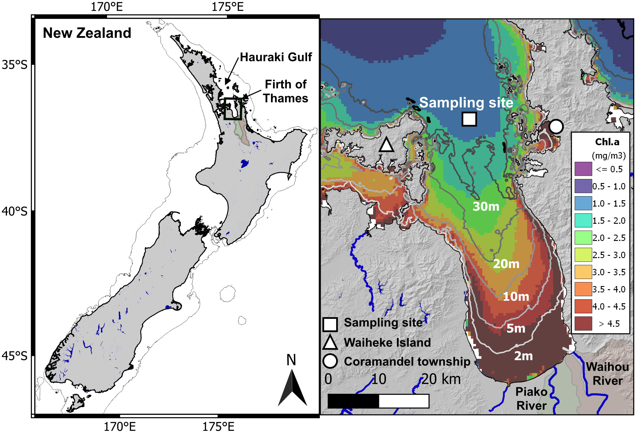
Figure 1 The Hauraki Gulf and Firth of Thames in northeastern Aotearoa New Zealand. The figure displays a map of New Zealand indicating the boundary of the continental shelf (200 m). The Firth of Thames is located at the southern end of the Hauraki Gulf and exhibits shallowing bathymetry towards the main river catchments, namely Waihou and Piako. The white square represents the in situ sampling site situated in the outer Firth at a water depth of approximately 35-40 m. The figure also presents the annual average climatology of surface Chl.a (mg m^-3) derived from satellite data (MODIS-Aqua), offering a spatial perspective of Chl.a distribution between the inner and outer regions of the Firth.

The productivity dynamics in the Firth are primarily driven by inputs of dissolved inorganic nitrogen (DIN) from the river catchments, particularly from the Waihou and Piako rivers located at the southern end (Zeldis and Swaney, 2018 and Zeldis et al., 2022). These riverine inputs, derived mainly from anthropogenic sources from historical agricultural development, contribute significantly to the productivity, accounting for approximately 85% of the total DIN input. In contrast, oceanic inputs from the northern Hauraki Gulf make up only a minor contribution of approximately 15% of the total DIN input.

Firth productivity is also influenced by seasonal and interannual variations in the vertical stratification of water column properties from freshwater inputs and temperature (Chang et al., 2003; Zeldis et al., 2004; Gall and Zeldis, 2011 and Zeldis et al., 2022). These variations play a crucial role in shaping the composition, abundance, and stratification of phytoplankton and zooplankton communities. The Firth experiences weak stratification during winter and spring, which intensifies during summer due to surface heating. In autumn, the water column starts to overturn due to cooling and decreasing freshwater inputs. As we move seaward into the Hauraki Gulf, the nutrient loading in this area is predominantly influenced by inputs from the adjacent continental shelf (Sharples and Greig, 1998; Zeldis et al., 2004, and Gall and Zeldis, 2011 and Bury et al., 2012). The variability of nutrients and productivity patterns in the Hauraki Gulf is shaped by shelf flows, including upwelling and downwelling dynamics. These flows contribute to the fluctuations in nutrient levels, playing a significant role in determining nutrient availability and influencing productivity patterns in the region.

Understanding the factors that drive productivity dynamics in the Firth of Thames and the adjacent Hauraki Gulf, is essential for effective management and conservation efforts in this ecologically important area. To achieve this, a dedicated effort was made over a decade-long period from 2005 to 2015 involving in situ collections (ship surveys and moored instrumentation) at the entrance to the Firth. This initiative had three main objectives: (1) validating the accuracy of satellite (MODIS-Aqua) Case1/Case2 blended products using NIWA-processing (Chl.a, C_phyt and light attenuation); (2) explore the complexities of stratification, seasonal predictability, patterns, and trends; and (3) testing the hypothesis that incorporating deep biomass corrections would significantly enhance the accuracy of NPP estimates obtained from satellite data. Our discussion addresses uncertainties associated with NPP models and provides a current contextual understanding of biomass stratification across the broader region. We take into consideration factors such as a shallowing continental shelf and the influence of both on- and offshore drivers.

2 Materials and methods

2.1 Seagoing sampling

Seagoing data for the present study were collected between mid-2005 (Jul.) and mid-2015 at the outer Firth monitoring site (Figure 1) over 40 voyages (predominately on NIWA’s RV Kaharoa but also using Western Work Boats Macy Gray and Star Keys). At approximately three-month intervals, seasonal voyages were undertaken to collect discrete biophysical data by deploying a Seabird SBE 911plus CTD (conductivity, temperature, depth) equipped with additional sensors for measuring Chl.a fluorescence (Seapoint Sensors Inc.), beam attenuation (CStar 660 nm, Wetlabs/Sea-Bird Scientific), and photosynthetically active radiation (PAR) using an LI-194 sensor (LI-COR Inc.). These measurements allowed for the profiling of water column properties. A rosette sampler with 12 x 10 L Niskin bottles fitted to the CTD captured water samples at six nominal depths (5, 10, 15, 20, 30 and 35 m) and processed according to methods detailed in Zeldis et al., 2022 and outlined below.

During each ship survey, a sub-surface mooring (Supplementary Figure 1A) equipped to measure water column biophysical properties was deployed, serviced, and subsequently re-deployed. Integrating Natural Fluorometers (INF-300, Biospherical Inc.) were positioned on the mooring to assess Chl.a (683 nm) and photosynthetically active radiation (PAR), within the upper surface mixed layer (~ 7 m) and deeper in the euphotic zone (~ 20 m) (see Chl.a methods below). The fluorescence and PAR sensors were kept free of biofouling using equipment that squirted saturated bromine solution on the sensor surfaces for 15 s every 3 h (Supplementary Figures 1B, C). Physical water column stratification was assessed using conductivity-temperature-depth-oxygen (CTDO) sensors (SBE 37 SMP-ODO, Sea-Bird Scientific) on the mooring within the mixed layer (~ 9 m) and near-bottom (~ 33 m) depths. All sensors sampled at 10-15 min intervals and daily means of data were used for comparison with seasonal ship survey and satellite observations.

2.2 Satellite observations

Remotely sensed data obtained from NASA’s Moderate Resolution Imaging Spectrometer (MODIS), on the Earth Observing System (EOS) Aqua satellite (MODIS-Aqua), were utilized in this study (c.f. Figure 2 data-processing workflow outlined in Gall et al., 2022). To summarize, the raw data was received through direct broadcast at the NIWA Lauder satellite receiver in Otago. Calibration was performed, and ocean colour product algorithms applied to the data. Subsequently, the data were interpolated to a spatial resolution of 500 m on a transverse Mercator grid. For an extended analysis covering the period from mid-2002 to mid-2018, data were extracted from a 3 x 3, 9-pixel area centered around the study site. Medians of the nine-pixel area were calculated to optimize accuracy of the central pixel value which was within 5% in 99% of cases. This approach also effectively increased the number of observations throughout the timeseries by minimizing pixel failure caused by factors such as cloud cover, shadows, and breaking waves. As a result, there were approximately 20% more days available for observations.

Figure 2

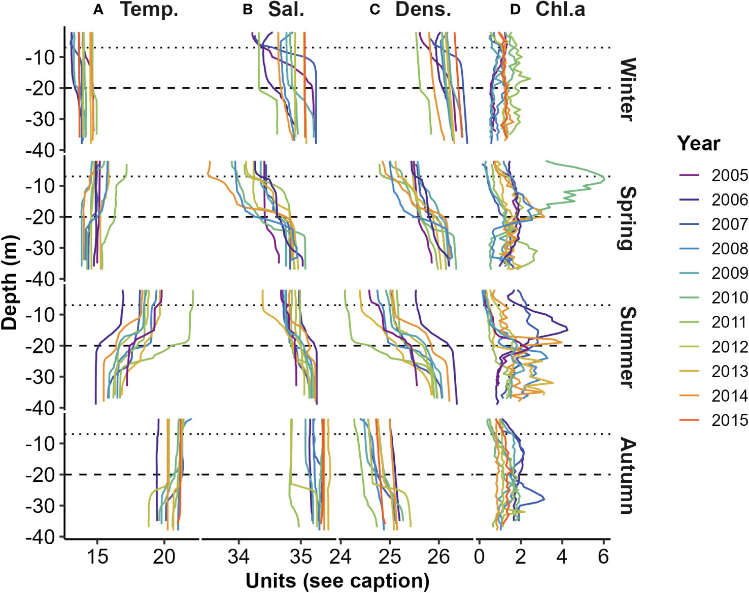
Figure 2 Seasonal water column stratification profiles obtained using CTD measurements: (A) Temperature (°C); (B) Salinity (ppt); (C) Density (kg m^-3); and (D) Chl.a fluorescence (mg m^-3). Dotted and dashed horizontal lines illustrate the nominal depths (7 m and 20 m) of the Chl.a sensing INF instruments (see Supplementary Figure 1A). Samples were collected during mid-winter (Jul.), mid-spring (Oct.), early summer (Dec.), and early autumn (Mar.).

2.3 Physical and optical properties

CTD profiles were employed to assess various physical (temperature, salinity, density) and optical (PAR) properties and identify boundaries within the water column. These included: the surface mixed layer depth (z_m, m), where the density exceeded 0.125 kg m^-3 that of surface values (Levitus, 1982); the bottom mixed layer depth (z_bm, m₎, where the density reduced by 0.125 kg m^-3 that of bottom measures; the pycnocline width (y_pw, m), the distance (m) between layer depths (z_bm– z_m); the scalar light attenuation of PAR (K_oPAR), from the slope of the natural log transformed PAR profile; and the euphotic zone depth (z_eu), at which light is 1% of sub surface levels (Kirk, 2011).

In relatively clear waters satellite downwelling light attenuation of PAR (K_dPAR) can be estimated from a simple empirical relationship (Morel et al., 2007) to the K_d490 band ratio algorithm product (Clark, 1997). In turbid waters a modified quasi analytical algorithm (QAA - Lee et al., 2005) from backscatter and the total absorption spectral coefficient is more accurate (Pinkerton, 2017). ‘Logistic-scaling’ of a backscatter product (b_bp555, m^-1) was used in a blended procedure to estimate K_dPAR across Case 1 and Case 2 conditions (Pinkerton, 2017 and Gall et al., 2022). The NIWA long term monitoring site (Figure 1) conformed to Case 1 conditions 98% of the time.

2.4 Phytoplankton biomass

2.4.1 Chlorophyll a

All water samples were filtered onto 25 mm glass fiber filters (GFF – Whatman International Ltd.) and stored frozen (-20 °C) prior to the analysis of Chl.a and its phaeopigments (Pha.a). Samples were also size fractionated onto a series of 47 mm polycarbonate (PC – Pall Corporation) filters (20, 5, 2 and 0.2 µm). Chl.a and Pha.a were extracted from the stored filters (grinding for GFF and shaking for PC) into 90% acetone, followed by soaking refrigerated (4 °C) in the dark (4-hr and overnight respectively). Concentrations were determined by fluorescence against an analytical grade Chl.a standard (96145 Sigma-Aldrich) before and after acidification according to the original methods of Holm-Hansen et al., 1965. The fluorescence spectrophotometer (Varian Carey Eclipse 11) was configured to minimize the interference from chlorophyll b and c, and their degradation products, by using a narrow-slit width (5 nm) for the excitation (431 nm) and emission (670 nm) wavelengths (e.g., Trees et al., 1985).

Estimates of Chl.a from moored INF’s followed the natural fluorescence calculations of Chamberlin et al., 1990. These are detailed further in Gall and Zeldis, 2011, with the following modifications: (1) K_oPAR estimates between moored INF’s were used instead of seasonal CTD K_oPAR; and (2) instead of using a mean absorption coefficient for phytoplankton, the light absorption coefficients of the phytoplankton were measured at INF depths from seasonal samplings, following a modified transmission-reflection method of Tassan and Ferrari, 2002, as follows: Triplicate water samples (up to 1 L) were filtered onto 25 mm GFF to an even and moderately intense colour, and the filter stored at -80 °C in flat perforated histology cases to avoid disturbing the surface sample. Samples were thawed and rewetted on microscope slides (inspected to ensure absence of bubbles) prior to measurements before and after algal pigment removal using an integration sphere attachment to a UV-VIS spectrophotometer (Shimadzu Inc.). Methanol, instead of bleach, was used to remove pigments (Kishino et al., 1985) prior to readings, as some freshwater studies have shown bleaching of ‘tripton’ in the non-algal particle fraction, which overestimates algal pigment absorption by difference (e.g., Binding et al., 2008). Phytoplankton (algal particles) absorption spectra (a_ap,m^-1) was obtained by difference between the total particulate spectra (a_p,m^-1) and the methanol extracted non-algal particle spectra (a_nap,m^-1).

The satellite Chl.a estimation method also utilized a blending technique that combined a Case 1 MODIS-Aqua product (NASA - R2018.0) with a Case 2 QAA (Lee et al., 2005 and Lee et al., 2007). The QAA product was employed to derive estimates of particulate backscattering at 555 nm (b_bp555) and phytoplankton absorption at 488 nm (a_phyt488). For the estimation of the Case 2 Chl.a product, Chl.a-specific absorption coefficients from various regions in New Zealand, including the dataset used in this study, were incorporated (Pinkerton, 2017). The ‘logistic-scaling’ approach was employed to blend the backscatter product (b_bp555) and estimate Chl.a under both Case 1 and Case 2 conditions (Pinkerton, 2017). This blending procedure allowed for an improved assessment of Chl.a concentrations using satellite data.

2.4.2 Phytoplankton cell carbon

Water samples collected from all depths were analyzed to determine the composition, abundance, and carbon content of phytoplankton species (refer to Safi et al., 2022 for detailed description of this analysis). In brief, water samples of 250 ml were preserved in Lugol’s iodine solution (final concentration of 1%) for the identification and enumeration of phytoplankton larger than 2 µm. Triplicate samples (2 ml) for picophytoplankton (<2 µm) were frozen in liquid nitrogen for flow cytometry-based counting, following the methods described in Hall et al., 2006, to distinguish between picoeukaryotes and picoprokaryotes. Phytoplankton species were enumerated and categorized into diatoms (including large centric and pennate forms), dinoflagellates (encompassing large motile armored, thecate, and naked types), and others (primarily nano-flagellates, silico-flagellates, raphidophytes, prymnesiophytes, cryptophyceae, chrysophyceae, euglenoids, and monads). The total biomass of phytoplankton carbon (C_phyt) was determined by summing the biomass of all the groups (calculated from measured biovolume estimates and published carbon-biovolume equations for taxa – see Safi et al., 2022). For the analysis of size-partitioning of C_phyt and the biomass ratio (C_phyt : Chl.a), micro-phytoplankton (>20 µm) mainly comprised the large centric diatoms and large armored dinoflagellates, while the remaining fraction, referred to as nano-phytoplankton (2-20 µm), included combined pennate diatoms, thecate and naked dinoflagellates, as well as small nano-flagellates and a few silico-flagellates. The contributions of the remaining groups to the total biomass were less than 0.1%.

The method proposed by Behrenfeld et al., 2005 introduced the estimation of satellite C_phyt based on an empirical relationship using backscatter coefficients of particulates. This relationship was further supported and updated by Graff et al., 2015, using more comprehensive studies encompassing various ecosystems:

$$C_{phyt} (mg m^{-3})= 12128(b_{bp}470- b_{bpnap}470)+ 0.59$$

As differences in b_bp wavelengths are relatively invariant across a range of marine phytoplankton cultures (Whitmire et al., 2010) we assumed this relationship was applicable to the b_bp555 wavelength which we used here.

2.5 Net primary productivity

2.5.1 VGPM

A vertically generalized production model (VGPM - Behrenfeld and Falkowski, 1997a), regionally tuned on previous studies (Gall and Zeldis, 2011), was used to estimate NPP from the optimum photosynthetic rate per unit Chl.a (P_bopt – mg C(mg Chl.a)^-1 h^-1) in z_eu, Chl.a [Chl.a_surf x z_eu – mg m^-2], day-length (DL - hr), and the light dependency function [fE_o= 0.66125E_o/(E_o+4.1)]:

$$VGPM (mg m^{-2} d^{-1})=P_{bopt} [Chl.a_{surf} x z_{eu}]x DL x f{E}_0$$

The values of P_bopt determined at the Firth monitoring site and the continental shelf edge (150 m depth) off northeastern New Zealand (Gall and Zeldis, 2011) exhibited a range of 1.5 to 6.0 mg C(mg Chl.a)^-1 h^-1. The dataset was too small to reliably estimate temperature dependency or seasonality in the parameter over the two years of sampling (n=11, from spring 1998 to summer 1999, 2 seasons each, except for winter). A mean P_bopt value (2.9) combined with satellite Chl.a and z_eu accounted for about 50% of the variability between VGPM and ¹⁴C shipboard incubations (Gall and Zeldis, 2011), similar to Behrenfeld and Falkowski, 1997b and Gall et al., 1999. The latter study in oceanic subtropical waters, north of the Chatham Rise, east of New Zealand (n =14) also lacked temperature or seasonal dependencies, ranging from about 1.2-7.6 (mean 3.7) mg C (mg Chl.a)^-1 h^-1.

To account for deep Chl.a in z_eu, we used mooring Chl.a (7 m and 20 m estimates) to calculate a correction factor (CF) for use with surface measures [Chl.a_surf x z_eu], and investigated its seasonality (month, t. CFm) with sine and cosine functions in regression analysis over a 12-month period (T) (Stolwijk et al., 1999). This provided a simple correction for VGPM that included deep biomass (db):

$$VGP{M}_{db}(mg m^{-2} d^{-1})= P_{bopt} [Chl.a_{surf} x z_{eu}]x CFm x DL x f{E}_0,$$

where $CFm (month, m)=A + \beta 1 x \sin \frac{2\pi t}{T}+ \beta 2 x \cos \frac{2\pi t}{T}$, derived from a regression on $CF= \frac{Chl.a(7m) x 20 + Chl.a(20m) x (z_{eu} - 20)}{Chl.a(7m) x z_{eu}}.$

The periodic regression can have more terms (β3 + β4) to account for periodicity over shorter time periods if significant, which was not the case in our data.

2.5.2 CbPM

In order to address physiological limitations in the VGPM, such as the challenge of accurately predicting seasonality in P_bopt, we used a carbon-based production model (CbPM) that relied on growth rate estimates, following the approach outlined by Behrenfeld et al., 2005). Using an equivalent formulation to the Chl.a VGPM, we estimated NPP based on C_phyt (C, mg m^-3) and growth rates (µ, divisions d^-1), assumed homogeneity throughout the euphotic zone (z_eu, m), which employed a dependent profile of C_phyt fixation [h(I_o)] that varied with light irradiance (I):

$$CbPM (mg m^{-2} d^{-1}) = {[\mu x C_{phyt} x z]}_{eu} x h(I_0),$$

where h(I_o) = f(E_o).

Growth rates are determined against maximum anticipated growth rates of 2 divisions d^-1, considering light, nutrient, and temperature adaptations of the Chl.a:C_phyt biomass ratio. The maximum Chl.a:C_phyt ratios are derived from empirical studies conducted by Behrenfeld et al., 2005 and Westberry et al., 2008:

$$\mu (divisions d^{-1})= \frac{2 x Chl.a:C_{phyt}}{Chl.a:C_{phyt}(max)}x (1-ex{p}^{-5I_g}),$$

where $Chl.a:C_{phyt}(max) = 0.022 + (0.045 - 0.022) ex{p}^{-3I_g}$, and $I_g (mol photons m^{-2} h^{-1}) = I_{0 } ex{p}^{-K_{d}490 x \frac{z}{2}}$

Downwelling light attenuation at 490 nm (K_d490) was estimated from the turbid water K_dPAR (>0.115 m^-1) relationship of Saulquin et al., 2013):

$$K_{d}490= {10}^{\frac{log10\left(\frac{K_{d}PAR}{0.81}\right)}{0.8256}}$$

Further improvements have been proposed for the CbPM in accounting for vertically resolved spectral irradiance photoacclimation and nutrient stress (nitrocline depth), by Westberry et al., 2008. We simplified their approach by accounting for C_phyt and growth rates in two layers, the upper mixed layer (z_m) and below mixed layer (z_bm) to the base of z_eu. The latter includes the biomass across the pyncoline width (y_pw):

$$CbP{M}_{db} (mg m^{-2} d^{-1}) = [{(\mu x C_{phyt} x z)}_m + {(\mu x C_{phyt} x z)}_{bm}] x h(I_0)$$

Seasonal vertical CTD profiles and mooring data were used in a periodic regression (Stolwijk et al., 1999) to determine seasonality of the depth of z_m (m) and pycnocline width (y_pw, m). Linear model regressions of seasonality of Chl.a:C_phyt(z_bm) from ship surveys, with the ratio of surface (7 m) Chl.a to that at 20 m from mooring datasets [Chl.aR(7m/20m)], were used to calculate C_phyt below z_m [C_phyt(z_bm)] from surface satellite Chl.a, and therefore Chl.a:C_phyt(z_bm).

2.6 Statistical analysis and graphics

Statistical analysis and graphics were performed using R software (RStudio-Team, 2022), except for location maps (QGIS, 2022). Many of functions are include in base R, including linear model regression (lm) and statistical analysis functions from the Stats package (3.6.2). Standardized Major Axis (SMA) linear regression was used to minimize total least squares (TLS - orthogonal) rather than ordinary least squares (OLS) for bivariate comparisons using the ‘smatr 3’ package (Warton et al., 2012). This Model II regression method accounts for errors in both x and y variables to ensure statistically robust analysis. Figures were constructed using the grammar of graphics ‘ggplot2’ package (Wickham, 2011), customized for publication ready plots using the ‘ggpubr’ package (Kassambara, 2020). Missing daily data (mooring and satellite) were linearly interpolated between nearest values for seasonal statistics and analysis using the approx. function in the base R Stats package.

3 Results

3.1 Physical and optical properties

Seasonal in situ collections [mainly in early autumn (Mar.), mid-winter (Jul.), mid-spring (Oct.), and early summer (Dec.)], profiled a range of water column physical properties and strengths of vertical stratification (Figure 2). Surface water column temperatures varied from mid-winter lows (about 13 °C) to highs (about 22 °C) in early autumn (Figure 2A). Surface salinities were generally lowest (<34.5 ppt) during mid-spring and highest (>35 ppt) during early autumn. The largest vertical difference in density stratification occurred in early summer (Figure 2C).

Consequently, surface mixed layer depth (z_m) and the pycnocline width (y_pw – in m not depth) were strongly and significantly seasonal (Figures 3A, B and Table 1). Generally, mixed layer depth (z_m) was shallow between spring and summer (<10 m) and deep during mid-winter (>20 m), while pycnocline width (y_pw) was large (~ 20 m) during spring-summer and small (~ 5 m) during mid-winter (Figure 3C) - although at times exceptions occurred with multi-step water column density profiles evident (Figure 2C). The depth of the euphotic zone (z_eu) and its relationship to z_m and the depth to the base of the pycnocline (z_pb = z_m + y_pw) are relevant in terms of light supply for phytoplankton growth (Figure 3D). In most cases z_eu is deeper than z_m and comparable to z_pb, but at times deeper than both - particularly from early summer to early autumn. Seasonality in z_eu was not statistically significant and could attest to high interannual variability and low sampling numbers (n = 10, years). There is an indication of seasonality, with depths being generally shallower in winter and spring months, and deeper during the summer and autumn.

Figure 3

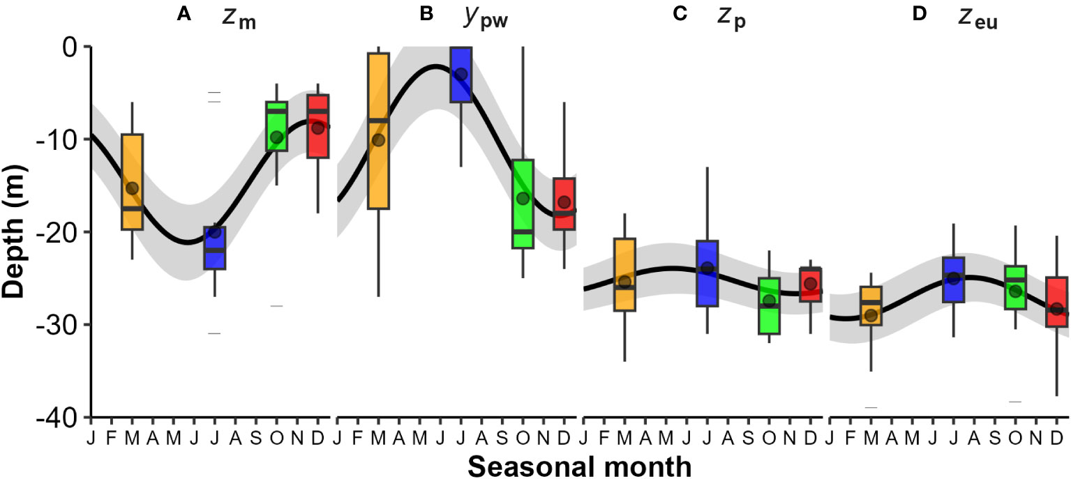
Figure 3 Seasonal variations in water column physical and optical layer depths from CTD profiles: (A) Mixed layer depth (z_m); (B) Pycnocline width (y_pw) in meters; (C) Base of pycnocline layer depth (z_{pb =} z_m + y_pw); and (D) Euphotic zone depth (z_eu). The boxplots illustrate the interquartile range (IQR - box), median line, mean point, 1.5 x IQR whisker, and extreme values (dashed lines). Seasonal categories are colour coded: Autumn (orange), Winter (blue), Spring (green), and Summer (red). Significant seasonality (black line) was observed for z_m and y_pw (Kruskall-Wallis test, p<0.05, see Table 1 for regression models).

Table 1

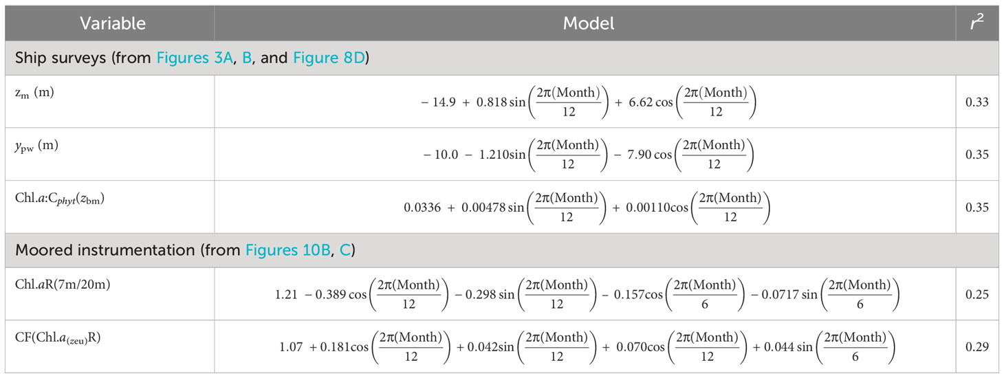
Table 1 Seasonal sinusoidal regression models of physical and biological features from seasonal surveys and moored instrumentation.

The time series of water column physical properties obtained from moored sensors and surface satellite products, collected on a quasi-daily basis (Figure 4), provides significantly higher statistical power compared to the seasonal voyage snapshots taken every three months. These continuous measurements more reliably captured the seasonal periodicity on a monthly scale, as illustrated in Figure 5. Satellite SST (Figure 4A) agreed well with mooring data (Figure 6A, r² = 0.91), although tended to have a slightly positive (higher) bias during summers and negative (lower) bias during winters, which may reflect different sampling depths (surface (<5 m) vs 7-10 m). Euphotic zone depth estimates from CTD and mooring data (Figure 4C) also agreed reasonably well (Figures 6B–D, r² = 0.55) although they differed at times. Satellite observations were like those from CTD profiles, with a small negative (lower) bias (Figure 6C), although regression and observation numbers are lower (r² = 0.44, n = 17). Mooring z_eu contained a higher number of matchups with satellite data (n = 981), no bias, but lower agreement (Figure 6D, r² = 0.26), which is not surprising considering the different depth ranges of estimates (surface optical depth<5 m vs a moored sub-surface 7-20 m assessment). Complex water column stratification in physical properties and multi-stepped surface layers (Figure 2) are likely to stratify light attenuating components across the water column such that at times, CTD, mooring and satellite observations sampled different surface layers.

Figure 4

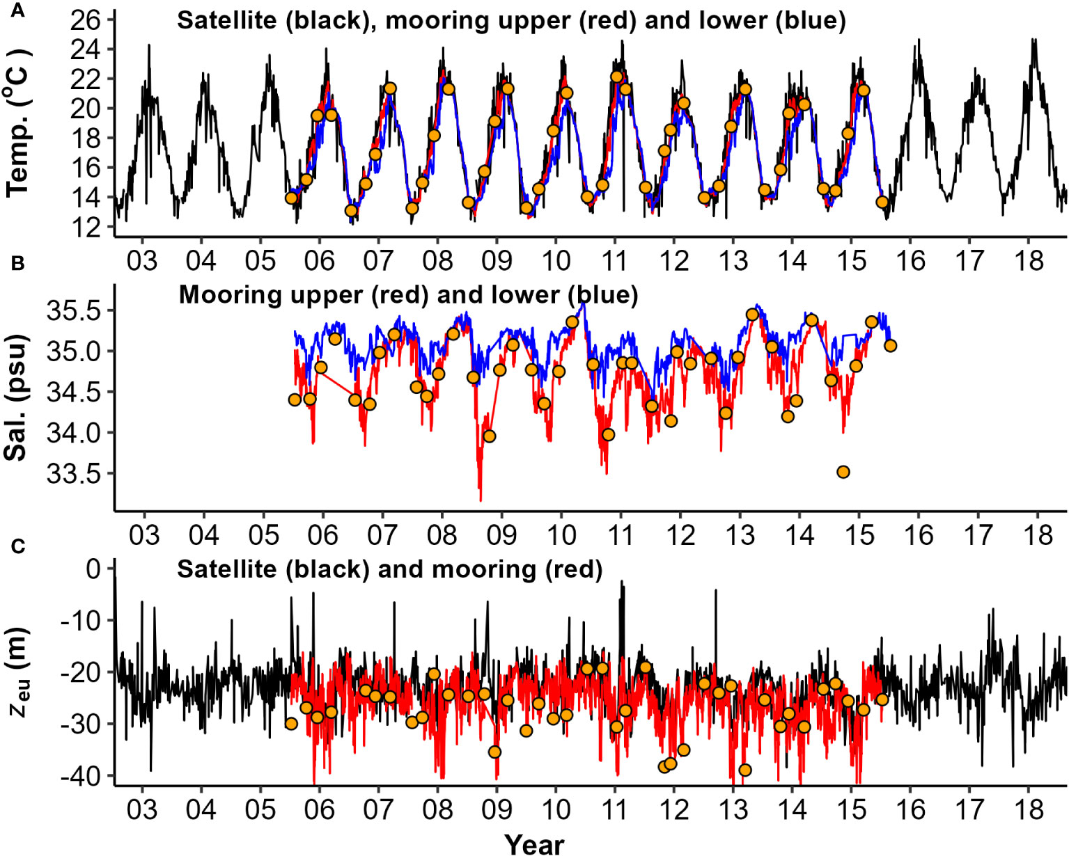
Figure 4 Water column physical and optical properties captured by moored sensors and satellite data: (A) Temperature (Temp.); (B) Salinity (Sal.); and (C) Euphotic zone depth (z_eu). Daily timeseries display upper (~ 7 m - red) and lower (~ 33 m - blue) mooring data, overlaid with MODIS-Aqua (black) and seasonal voyage data from CTD casts (orange points).

Figure 5

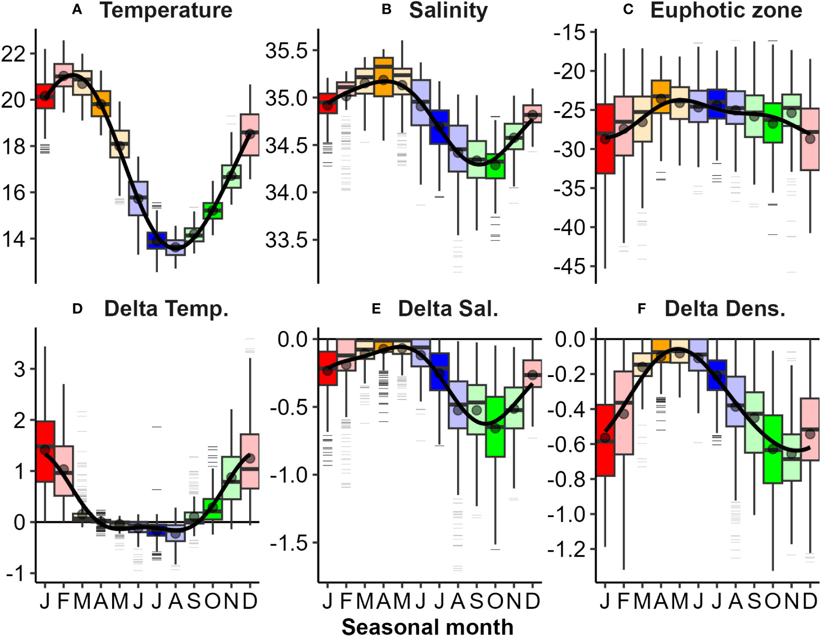
Figure 5 Seasonal variations in physical and optical properties and their stratification observed from mooring data: (A) Temperature (°C); (B) Salinity (ppt); (C) Euphotic zone depth (m); and differences (Delta) between upper (~ 7 m) lower (~ 33 m) properties for (D) Temperature; (E) Salinity; and (F) Density (kg m^-3). Horizontal black lines on panels (D–F) highlight no stratification. Seasonality was significant for all variables (Kruskall-Wallis test, p<0.01). Please refer to the caption of Figure 3 for boxplot details.

Figure 6

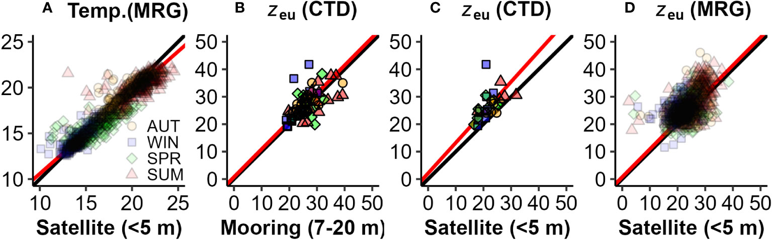
Figure 6 Comparisons between CTD, mooring (MRG) and satellite physical properties: (A) Mooring vs Satellite temperature [y = 0.89x + 1.6, r² = 0.91, n = 1200, p<0.001]; (B) CTD vs Mooring z_eu [y = 1.01x + 0.87, r² = 0.55, n=40, p< 0.001]; (C) CTD vs Satellite z_eu [y = 1.1x + 1.4, r² = 0.44, n = 18, p = 0.002); and (D) Mooring vs Satellite z_eu [y = 1.16x – 1.21 r² = 0.26, n = 1103, p< 0.001]. The 1:1 relationship (black) generally aligns with the standardized major axis regression (red), except in (C) when number of observations and range of data are low.

All physical properties derived from mooring observations were seasonally significant in their periodicity regression models (Figure 5). Mooring surface temperature was highest in late summer and lowest in late winter (Figure 5A). Surface salinity was highest in mid-autumn and lowest in mid to late spring (Figure 5B). Water column stratification was (generally) weakest during late autumn, and strongest during late spring (Figure 5F). There were obvious extremes and exceptions in patterns (e.g., lowest surface salinity water (<32 ppt) and largest salinity gradient (>1.5 ppt) during late winter 2008 (Figure 4B), coinciding with a flood event on 30-July-2018 (Supplementary Figure 2B). Other large flood events (e.g., Jan 2011 and 2012) also have low surface salinity, and both surface and deep salinities stayed generally lower during summers of these years compared with other years (Figure 4B). The lowest surface salinities observed during mid to late spring were typically delayed by approximately 1-2 months from the peak river flows that occurred in late winter (Supplementary Figure 2B). Euphotic zone depths in mooring records ranged from at least the maximum depth of the water column (about 40 m) to as shallow as 5-10 m in satellite records (Figure 4C). Strong z_eu seasonality was evident in mooring records across the year, with clearest waters (deepest euphotic zones) in mid-summer and more turbid waters (shallower euphotic zones) in mid-autumn; however, there was also considerable variation within months among years (Figure 5C). Shallower z_eu events (5-10 m) in satellite observations (2007, 2008 and 2009) than in mooring records (Figure 4C), coincided with near-surface salinity decreases (Figure 4B).

3.2 Phytoplankton biomass

Seasonal CTD profiles of Chl.a (from fluorescence) spanning the period from 2005-2015, exhibited depth-dependent variations that coincide with physical stratification patterns (Figure 2D). During early summers, subsurface maxima layers (SCML) often formed at the base of the mixed layer or within the pycnocline, with high Chl.a values in the lower portion of the water column (HCL) compared to high Chl.a in the upper layer (HCU) - with an exception in 2006. Winter profiles generally had no SCML and associated with weak vertical physical stratification. Autumn and particularly spring, displayed a mix of higher Chl.a in upper and lower layers, with and without SCML at times.

Seasonal depth patterns are similar in the concentrations of phytoplankton biomass markers from water collections (Figures 7, 8). The distribution of Chl.a is like C_phyt above z_m but not below (white line, Figures 7A, C). In general, C_phyt : Chl.a is higher above z_m (>50) than below (<50) (Figure 7D). High proportions of phaeopigment (Pha.a) highlight periods of senescence and decay (Figure 7B), which tended to occur in low Chl.a periods (i.e., generally opposite patterns to that of Chl.a - Figure 7A). Further details on the size-partitioned of phytoplankton biomass are provided in Supplementary Figures 3–5.

Figure 7

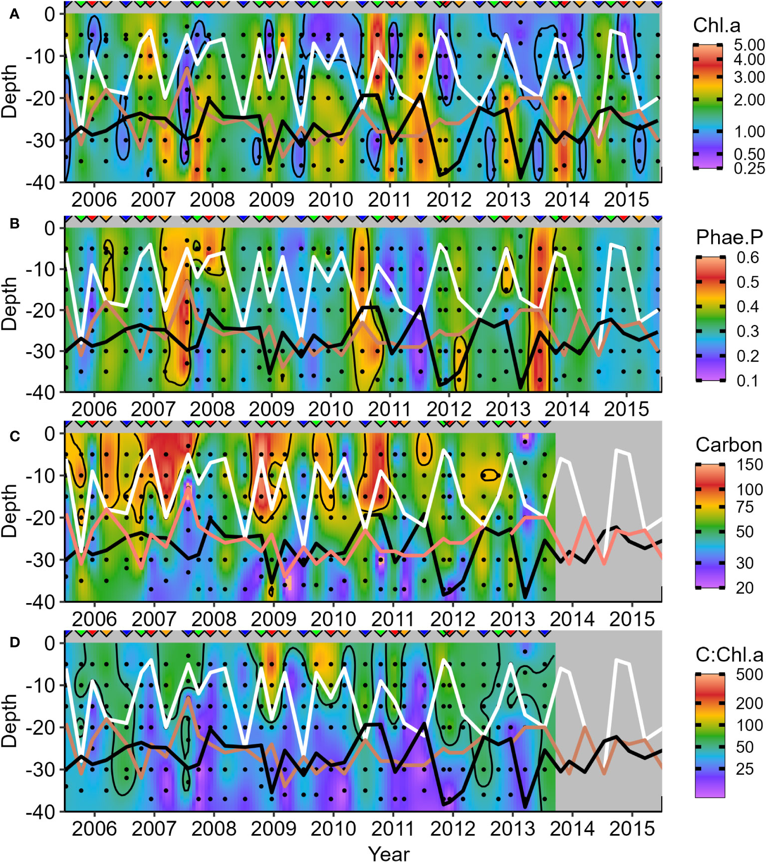
Figure 7 Seasonal variations in phytoplankton biomass markers in the water column during surveys: (A) Chlorophyll a (Chl.a); (B) Phaeopigment a Proportion [Pha.a:(Pha.a + Chl.a)]; (C) Carbon (C_phyt); and (D) C_phyt : Chl.a ratio. White lines represent mixed layer depth, salmon lines indicate the base of the pycnocline, and black lines represent the base of the euphotic zone. Upside-down triangles denote the seasonal timing of surveys (Winter – blue, Spring – green, Summer – red, and Autumn – orange). The winter of 2011 was unusual, with bottom Chl.a below z_eu and lower z_eu due to high surface Chl.a.

Figure 8

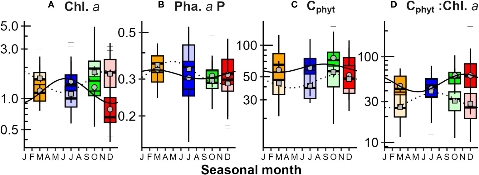
Figure 8 Seasonal variations in phytoplankton biomass above and below the mixed layer depth (z_m): (A) Chlorophyll a (Chl.a - mg m^-3); (B) Phaeopigment a Proportion [Pha.a:(Pha.a + Chl.a)]; (C) Carbon (C_phyt - mg m^-3); and (D) C_phyt : Chl.a (ratio). Bright boxes, circles and solid lines represent values above z_m, while light boxes, squares and dotted lines represent below z_m. Seasonality was statistically significant (p<0.05 Kruskall-Wallis test) for Chl.a both above and below z_m, Pha.a P below z_m and C_phyt : Chl.a below z_m. The seasonal variability Chl.a:C_phyt below z_m was utilized in the CbPM_db (deep biomass) modelling (see Table 1 for details). For additional information, refer to the caption of Figure 3.

Applying averaging to water column sections above and below the depth of the mixed layer (z_m) provided a clearer depiction of seasonal patterns (Figure 8). In early summer, above z_m, low Chl.a (Figure 8A, ~0.6 mg m^-3) occurred with high C_phyt (Figure 8C), resulting in the highest C_phyt : Chl.a ratios (Figure 8D, ~60). While the seasonality of the total biomass C_phyt : Chl.a ratio in surface waters was not significant (likely due to high interannual variability, and/or opposing size group effects), it was observed for pico-phytoplankton, with the highest ratios occurring in spring and summer (Supplementary Figure 5H). C_phyt was higher above z_m than below, especially from mid-winter to mid-spring (Figure 8C). Lowest concentrations of C_phyt occur below z_m in mid-winters (~40 mg m^-3), and above z_m in early summers (~60 mg m^-3). Chl.a and C_phyt seasonality patterns are similar below z_m. Seasonality was only significant for Chl.a above z_m, and Chl.a, Pha.a and C_phyt : Chl.a below z_m. The significant seasonal regression of the inverse ratio (Chl.a:C_phyt), as presented in Table 1, was utilized in the deep biomass CbPM_db-NPP modeling.

Phytoplankton biomass (Chl.a and C_phyt) from mooring (7 and 20 m) and satellite surface (<5 m) data, ranged from about 0.3-7.5 mg Chl.a m^-3 and 50-500 mg C_phyt m^-3 (Figure 9). Although satellite Chl.a was generally lower than mooring Chl.a (Figure 9A), seasonal patterns were similar, with high median concentrations during winter months and low concentrations during summer months (Figures 10A, D). Mooring Chl.a seasonality show a tendency for mid-autumn and late winter to early spring peaks, from a depression in early winter (Figure 10A), not seen in the more pronounced satellite seasonal cycle (Figure 10D). The ratio between upper (7 m) and lower (20 m) mooring Chl.a captured biomass-stratification seasonality, with high upper column Chl.a from autumn to spring (peaking in winter), to high lower column Chl.a from spring through summer (peaking in mid-summer) (Figure 10B; Table 1). Estimates of euphotic zone Chl.a from mooring surface Chl.a, and surface and deep Chl.a, were used to estimate a correction factor to apply to satellite surface Chl.a (Figure 10C; Table 1), to account for deep Chl.a in models.

Figure 9

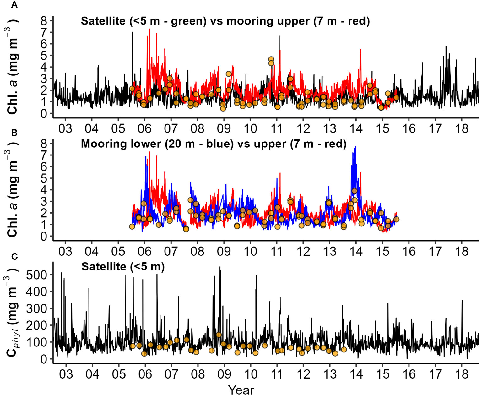
Figure 9 Daily timeseries of phytoplankton biomass from mooring and satellite observations: (A) Chlorophyll a (Chl.a) from satellite and upper water column mooring; (B) Chl.a from both upper and lower mooring depths; and (C) Carbon biomass (C_phyt) from satellite data. Seasonal collections from CTD depths are indicated as points.

Figure 10

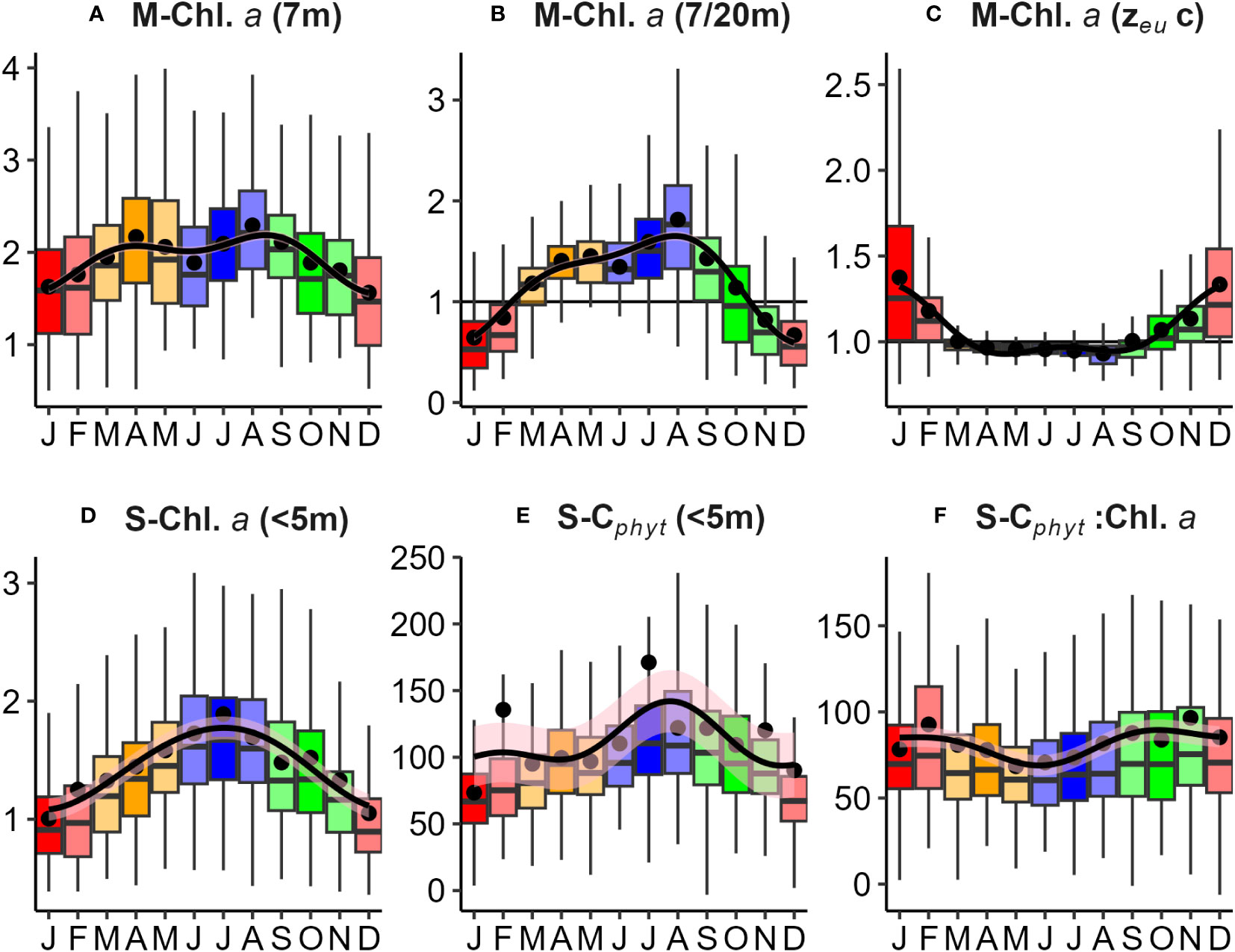
Figure 10 Seasonal variations in phytoplankton biomass observed from mooring (M) and satellite (S) data: (A) Mooring chlorophyll a (M-Chl.a - mg m^-3) at 7 m depth; (B) Ratio of mooring Chl.a between 7 and 20 m depths; (C) Euphotic zone correction factor for mooring Chl.a measurements to account for deep (>20 m) biomass within zeu (Table 2); (D) Satellite surface (< 5m) Chl.a (S-Chl.a - mg m-3); (E) Satellite carbon biomass (S-C_phyt– mg m^-3); and (F) Satellite C_phyt : Chl.a ratio. Seasonality was found to be significant (p<0.05 Kruskall-Wallis test) for all mooring and satellite measures. Note: The black horizontal line (B, C) represents a value of 1, indicating non-biomass stratified (well-mixed) conditions, where Chl.a (7m) is approximately equal to Chl.a (20 m).

Phytoplankton carbon (C_phyt) from satellite estimates (Figure 9C) had similar average magnitude as near-surface C_phyt from seasonal surveys (Figure 8C) with finer temporal resolution. Satellite estimates had significant periodicity, peaking in mid-late winter, and low during summer (Figure 10E). Surface biomass C_phyt : Chl.a ratios (Figure 10F) are similar in range and seasonality to those from seasonal surveys (Figure 8D), with significant (but low) seasonal periodicity. Biomass C_phyt : Chl.a ratio medians were generally low in early winter and high from spring through summer, although there was a large range of observations within months across the timeseries. Chl.a from mooring instruments agreed reasonably well with seasonal collections, with a small positive bias in near surface estimates (Figure 11A, r² = 0.27). Less bias occurred in deeper (20 m) estimates (Figure 11B, r² = 0.27). Chl.a from collections and from satellite (both from<5 m depth) had reasonable correlation (r² = 0.61) despite them having a limited number of satellite matchup days (Figure 11C, n=26). Satellite and mooring Chl.a were significantly correlated but have low confidence (r² = 0.18), with a small positive bias (Figure 11D). Correlations of C_phyt from seasonal collections with satellite estimates were weak (r²= 0.01, p=0.25), potentially due to the low number of observations (Figure 11E, n = 16). For spring, summer, and winter there were suggestions of positive relationships, but not for autumn.

Figure 11

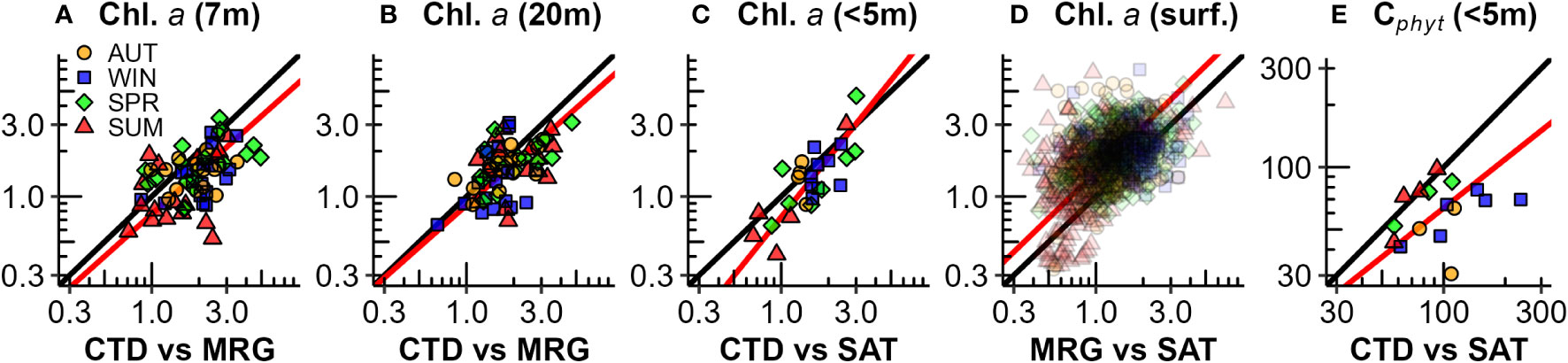
Figure 11 Comparisons of phytoplankton biomass between CTD rosette 3-month seasonal samplings, mooring (MRG) and satellite (SAT) estimates: (A) Chl.a CTD vs mooring upper (7 m) water column [y = 1.15x – 0.19, r² = 0.27, p<0.001, n = 67]; (B) Chl.a CTD vs mooring lower (20 m) water column [y = 0.92x – 0.06, r² = 0.27, p<0.001, n = 66]; (C) Chl.a CTD vs satellite [y = 1.3x – 0.13, r² = 0.61, p<0.001, n = 26]; (D) Chl.a Mooring (7 m) vs satellite [y = 1.01x + 0.16, r² = 0.18, p<0.001, n = 1116]; and (E) C_phyt CTD vs satellite [y = 0.78x + 0.23, r² = 0.01, p = 0.25, n = 15]. The scales are log₁₀ transformed.

3.3 Net primary productivity

The Chl.a- based vertically generalized production model (VGPM) and the C_phyt based model (CbPM) supply two insights into assessing NPP from satellite surface data at the site (Figures 12A, B). Total annual NPP (integrated between yearly mid-winters (July) to span the production growth cycle) averaged between 220 g C m^-2 y^-1 and 161 g C m^-2 y^-1 for VGPM and CbPM respectively (Table 2). Both models captured interannual variability of between about -10% to 10% of their overall annual climatological mean (Table 2) and showed strong seasonality (Figures 12C–F). The VGPM annual mean results were about 36% higher than the CbPM, with less seasonality, mainly from much higher production rates in winter months and only slightly higher production rates during summer months. Both models assumed a degree of predictability between surface measure and areal z_eu estimates, which is clearly not the case at times at this site (Figure 7; Supplementary Figures 7, 8).

Figure 12

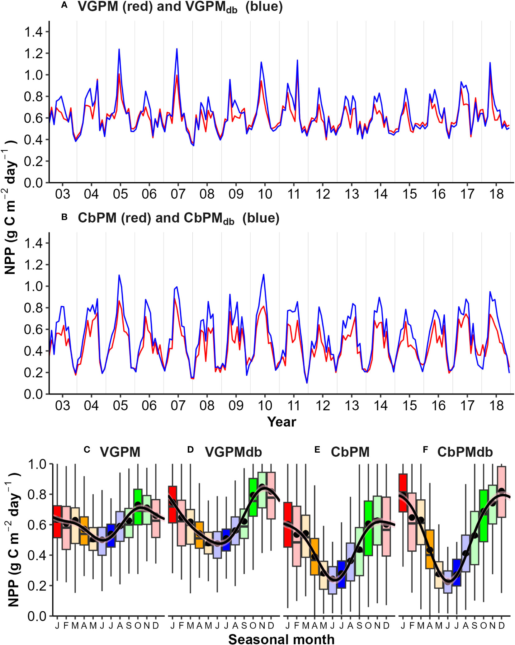
Figure 12 Comparison of Net Primary Productivity (NPP) models: (A) VGPM and VGPM_db (deep biomass corrected); (B) CbPM and CbPM_db; and (C–F) Seasonality. Seasonality was significant (p<0.05 Kruskall-Wallis test) for all measures.

Table 2

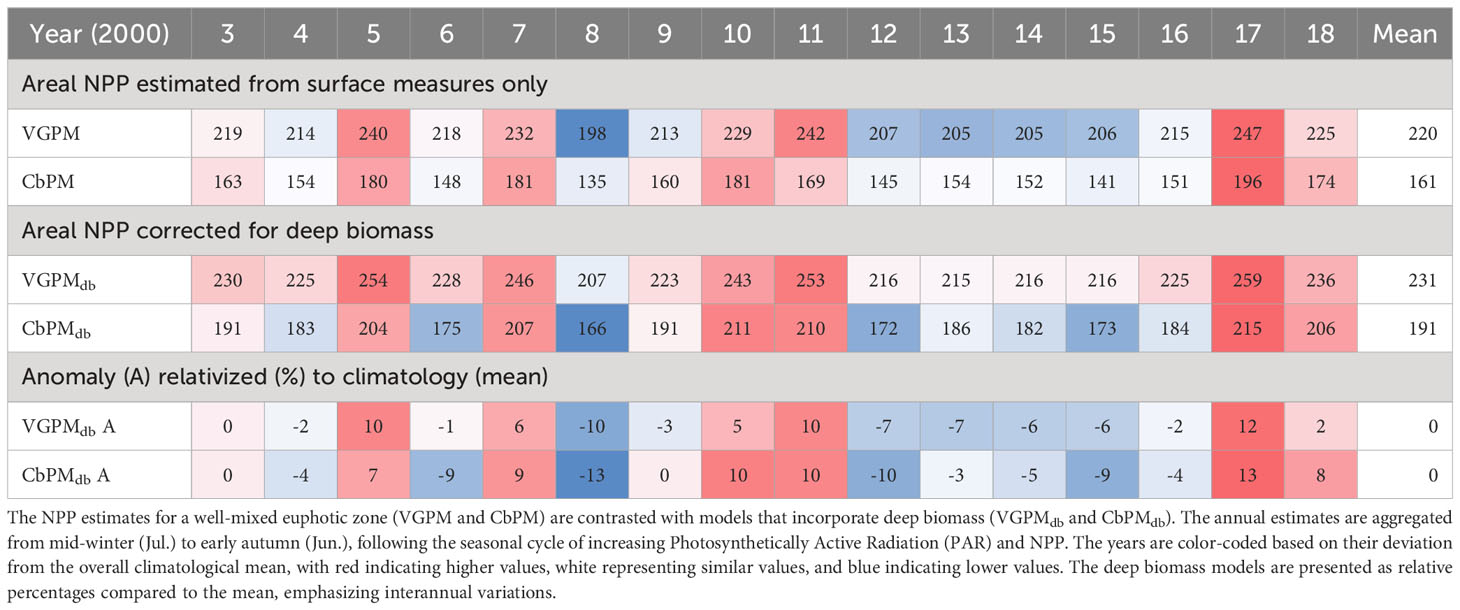
Table 2 Comparison of annual Net Primary Productivity (NPP) from satellite data.

To account for deep biomass not detected in surface measures (and lack of predictability in areal euphotic zone estimates (Supplementary Figures 7, 8), we used the mooring Chl.a stratification (7m/20m) seasonality regression (Table 1) to establish a seasonal correction factor (CF) for z_eu in the deep biomass VGPM_db model (Figure 12A), and a seasonal correction factor [Chl.a:C_phyt(z_bm)] (Table 1) for deep carbon biomass in the CbPM_db model (Figure 12B). Accounting for deep biomass increased total annual NPP to between 231 g C m^-2 y^-1 (a 5% increase) and 191 g C m^-2 y^-1 (an 18% increase) for VGPM_db and CbPM_db respectively (Table 2). Seasonally, accounting for deep biomass ranged from no change from mid-autumn to early spring, to largest increases during a late-autumn to an early summer peak for the VGPM (about 30%) and an early to mid-summer peak for the CbPM_db (about 33%).

4 Discussion

Our study investigates the impact of vertical stratification in a deep estuary site on the accuracy of satellite observations of water column biomass and net primary productivity (NPP). By incorporating seasonal vertical patterns of biomass, we improve (increase) the NPP satellite estimates. We examine the influences of observational representativeness, observational accuracy (between satellite, mooring and water collection measures), stratification, and seasonality on biomass and NPP estimation. We discuss NPP patterns in relation to previous observations and biomass trends (Safi et al., 2022) in the Firth, aiming to enhance satellite estimates across the broader region to the continental shelf edge.

To effectively capture the dynamic nature of the coastal ocean, we employed a range of observational methods that span representative space and time scales, enabling us to capture biogeochemical dynamics that are on par with the physical processes (Dickey, 2006). Our approach combines the temporal advantage of moored instruments (days-decades), highly time and space-resolved satellite observations (local-regional-continental), and vertical resolution from seasonal CTD-based surveys to gain synoptic insights. We discuss the factors affecting satellite information accuracy and explore the relationships and comparisons between these diverse data sources. However, assessing accuracy is challenging due to the differing sampling scales, which can lead to temporal decoupling, particularly in the case of satellite observations under cloudy conditions.

4.1 Representativeness and accuracy

Pinkerton et al., 2018 conducted an analysis of the accuracy of the MODIS-Aqua products utilized in our study region, offering valuable insights into satellite remote sensing of coastal water quality in the area. Furthermore, Gall et al., 2022 provides an overview of satellite remote sensing of coastal water quality in New Zealand, discussing both advances and challenges in this field, thus providing a broader context for our study.

It is worth noting that our moored instruments experienced tidal-driven depth variations of up to about 2.5 meters. The observed surface optical depths by the satellite, which were less than 5 meters, likely sampled shallower layers during periods of near-surface stratification compared to the moored instruments, which reached depths of around 7.5-10 meters. This phenomenon was evident at times in the CTD profiles depicted in Figure 2 and is supported by more detailed investigations into surface responses during discharge events within the Firth (Ø’Callaghan and Stevens, 2017).

Like other studies, our analysis reveals good agreement between sea surface temperature (SST) from satellite observations and in situ measurements. For instance, along the Korean Peninsula coast, Woo and Park, 2020 reported consistent results. Despite potential variations in assessment depths, we also found reasonable agreement in light attenuation (euphotic zone depth), with no evident seasonal bias. These findings align with comparisons made between satellite inherent optical properties (IOP) and field measurements in the China Sea, as demonstrated by Shang et al., 2011.

Our study revealed reasonable agreement among phytoplankton chlorophyll estimates obtained from 10 years of seasonal sampling voyages, moored instruments, and satellite observations, also without any notable seasonal bias (Figure 11A). However, there were discrepancies in the accuracy of the satellite and moored observations, with generally higher estimates from the mooring data, except for a few instances of low concentrations during summers. As highlighted above, differences may arise from variations in sampling depths, but also could be from methodological disparities between natural fluorescence measurements and satellite algorithms utilizing band ratio and absorption techniques. The mooring-based measurements of natural fluorescence were derived from daily averages which are known to include varying degrees of photochemical and non-photochemical quenching (Chamberlin et al., 1990). These quenching effects have the potential to influence the accuracy of the measurements.

Our satellite estimates of phytoplankton carbon, utilizing the empirical backscatter relationship of Graff et al., 2015 in the open ocean, demonstrated some agreement with in situ collections during mid-spring and early summer. However, in early autumn and mid-winter, the satellite estimates exhibited higher values. This higher bias coincided with periods when river stormflows, containing high loads of suspended mineral particles, were also seasonally high, potentially influenced the study site (see Supplementary Figure 1B). It is well known that changes in the contribution of non-algal particles, including inorganic and organic particles (detritus), to the backscatter signal can introduce a positive bias (Stramski et al., 2004). Additionally, closer agreement and lower error has been observed when small pico-phytoplankton dominate biomass (Bellacicco et al., 2020), which supports our high pico-phytoplankton biomass and their ratios during mid-spring and early summer (Supplementary Figures 8, 9) and better agreement during these seasons than others.

Considering that the Case 1/Case 2 logistic scaling of backscatter for the site indicated Case 1 conditions 98% of the time, we conclude that our phytoplankton biomass products have similar accuracy to open ocean estimates most of the time. Further confidence in the estimates’ reasonableness is supported by similar biomass C_phyt : Chl.a ratios compared to in situ measurements (as shown in this study against others, Supplementary Figure 9). Additionally, our findings align with similar seasonal patterns observed in other satellite studies conducted in the South China Sea (Xu et al., 2021), surface coastal stations in the Black Sea (Stelmakh and Gorbunova, 2018, and Stelmakh, 2020), temperate Danish coastal waters (Jakobsen and Markager, 2016), and conservative agreement with data from the northwestern Atlantic (Sathyendranath et al., 2009).

4.2 Biomass stratification and seasonality

The characterization of Chl.a stratification in coastal waters into different types, as presented by Zhao et al. (2019) for the German Bight, was observed at our study site. Our analysis of Chl.a biomass data obtained from mooring records yielded detailed monthly statistical distributions and boxplots that revealed consistent seasonal shifts in the distribution of Chl.a within the water column.

In early autumn to early spring, high Chl.a concentrations were predominantly found in the upper portion of the water column (HCU), while in late spring to late summer, they shifted to deeper regions either with a sub-surface maxima (SCML) or high Chl.a in the lower portion of the water column (HCL) to the bottom. These patterns were closely associated with the availability of dissolved macronutrients (Supplementary Figure 6), primarily by inorganic nitrogen (DIN), including nitrate N and ammonium N, as reported by Zeldis et al., 2022 and Safi et al., 2022, modified by variations in light and physical stratification as discussed in Gall and Zeldis, 2011 and Zeldis et al., 2022. Surface DIN concentrations remained consistently low, below 1 μmol L^-1, throughout the seasons, except for early winter when they exceeded 1 μmol L^-1. This threshold indicates the potential for nitrogen limitation according to Eppley et al., 1969. Zeldis et al. (2022) and Safi et al. (2022) offer a comprehensive examination and insightful discussion of the alterations in DIN, dissolved reactive phosphorus (DRP), and silicate (DRSi) concentrations, shedding light on the nuanced connections between these changing ratios and shifts in phytoplankton taxonomic groups within the region. Despite the low DIN levels, the shallow stratified surface layers received sufficient light for biomass accumulation, peaking from late winter to early spring as light intensity increased. As DIN became depleted in the surface layer and temperature stratification strengthened and deepened from spring into summer, biomass accumulated in the pycnocline, progressing deeper into the lower water column (HCL) where DIN levels were not limiting (>1 μmol L^-1), and with sufficient light in clear surface waters (deep euphotic zones) and increasing light, would support biomass. Zhao et al., 2019 observed deep HCL layers during the decay phase of the spring bloom, associated with resuspension and erosion of the SCML, yet recognized the potential for photosynthetic activity below the pycnocline.

In a recent study spanning from March 2015 to October 2017 (c.f. Figure 9; Zeldis et al., 2022), the use of moored oxygen sensors at a depth of 35 m revealed a pronounced peak in gross primary productivity (GPP) in the deep layer during summers. This peak coincided with the highest positive values of apparent oxygen utilization, an indicator of net respiration, occurring prior to the breakdown of water column stratification in early autumn. As light levels decreased from mid-summer through autumn, deep biomass layers would become light limited. During the autumn to winter period, complete mixing of the water column occurred, as depicted in Figure 5 (and described by Zeldis et al., 2022 in their Figures 7, 9), facilitating the replenishment of nutrient-depleted surface waters with macro-nutrients, completing the seasonal cycle.

The absence of cell senescence during mid-spring to early summer 3-month collections was supported by low phaeopigment ratios [Pha.a/(Chl.a + Pha.a)] that peaked in autumn and tended to be lowest in spring, albeit with interannual variability (Figure 8B). Safi et al., 2022 provided a detailed discussion on the development of a more heterotrophic system in early autumn, attributing the high ratios to the mineralization of spring primary production sometime during the mid-summer to early autumn period.

As well as nutrient supply and physical processes such as stratification, mixing and advective mechanisms influencing phytoplankton biomass and its stratification (Cullen et al., 2002), grazing, sedimentation, and cell lysis are also important mechanisms (Brussaard et al., 1995). Grazing pressure may also play a role in driving the formation and deepening of the deep Chl. a maxima (DCM) in the open ocean (Moeller et al., 2019), and previous studies in the inner Hauraki Gulf (Zeldis and Willis, 2015) showed increased rates of mesozooplankton grazing between spring and summer surveys that could add to biomass export to deeper layers.

An important distinction of deep Chl. a maxima DCM (SCML and/or HCL) is whether it is deep phytoplankton carbon (C_phyt) biomass maxima (DBM) or deep photoacclimation maxima (DAM) - Cornec et al., 2021. Although we only documented SCML on some occasions in CTD profiles (Figure 2D), it is relevant to HCL at this deep estuary site (or conversely, shallow continental shelf site) in photoacclimation seasonality observed in our low C_phyt : Chl.a ratios in early summer (Figure 8D). As highlighted above, it was plausible that there was sufficient light (at times) to support deep HCL phytoplankton growth and maintenance, where increasing pigment concentration per cell in light limiting conditions is an adaption to harvesting more energy for photosynthesis (Geider et al., 1998 and MacIntyre et al., 2002). HCL at the Firth of Thames site coincided with clear surface waters and deep euphotic zones up to the mid-summer period of highest light intensities (Figure 10B).

In comparison to the study by Gall and Zeldis, 2011, our investigation provided a more comprehensive understanding of the seasonal dynamics of phytoplankton biomass in this deep estuary site. We detected significant seasonal variations in biomass ratios of pico-phytoplankton (mainly Prochlorococcus) in surface waters at our site, with minimum values in winter and maximum values in summer (Supplementary Figures 6–7). Similar observations of larger sinusoidal variation were reported at the Hawaii Ocean Time-series (HOT) oligotrophic site in the North Pacific Gyre by Winn et al., 1995, as well as in satellite-based measurements of biomass ratios in the broader area around the HOT site (Westberry et al., 2016, c.f. Figure 2). Our research (Safi et al., 2022) also revealed an increase in micro-sized biomass during early summer and pronounced seasonality in deep biomass ratios, predominantly associated with micro-phytoplankton, originating from large centric diatoms and flagellates. The seasonal taxonomic shifts observed at our site may indicate that large motile phytoplankton with buoyancy control or flagella possess an advantage in exploiting nutrient gradients and light conditions during late spring and summer, as highlighted in studies by Sommer et al., 2017. It is well-known that diatoms, especially large centric diatoms, can rapidly adjust their sinking behaviors in response to changes in nutrient concentrations, as demonstrated by Du Clos et al., 2021.

4.3 Net primary productivity models

The mean annual Chl.a based, and deep biomass corrected, VGPM-NPP (220-231 g C m^-2 y^-1 respectively) from July-2002 to July-2018 was higher than previous estimates (Gall and Zeldis, 2011) using a similar model from 1998 and 2000 (178 g C m^-2 y^-1). We attribute this difference to lower Chl.a estimates resulting from a larger averaging area that included deeper Hauraki Gulf waters (Figure 1 vs c.f. Figure 1; Gall and Zeldis, 2011), rather than lower Chl.a at the Firth site.

In our study we used a fixed value of P_bopt (2.9 mg C (mg Chl.a)^-1 h^-1) determined in Gall and Zeldis (2011). It is important to note that P_bopt is known to be temperature dependent according to the findings of Harding et al. (2020). Although no seasonality was observed over the 13-23°C seasonal temperature range at the Firth monitoring site (Gall and Zeldis, 2011), this is likely due to the limited number of observations. If a greater availability of P_bopt data, like the findings in Harding et al. (2020) for Chesapeake Bay, had been present in our study, indicating a Pbopt range of 2.4-5.5 mg C (mg Chl.a)^-1 h^-1 across the 13-23 °C temperature range, it is likely that our analysis would have revealed more pronounced seasonality in VGPM-NPP.

The 25% lower CbPM-NPP models (161-191 g C m^-2 y^-1) are likely from lower growth estimates during the winter months, approximately half of those projected by the VGPM model. CbPM models are anticipated to better capture photoacclimation and physiological changes in C_phyt : Chl.a (Behrenfeld et al., 2005 and Westberry et al., 2008), rendering them more responsive to seasonal dynamics driven by factors such as nutrients and light, which have a significant influence on growth, supporting the larger range in seasonality of our CbPM models (Figure 12).

Productivity models that incorporate depth-dependent responses of phytoplankton biomass and physiology to subsurface irradiance are generally considered more accurate in the deeper open ocean. However, these models only explain approximately 15% more variance in in situ NPP estimates compared to surface based VGPMs and CbPMs (Behrenfeld and Falkowski, 1997a and references therein). In our study, we incorporated stratified biomass and seasonality in deep Chl.a layers using mooring observations, which supported this finding, resulting in a modest increase of annual NPP estimates by 5% to 18% for VGPM and CbPM, respectively. Although one represents variance explained and the other represents an increase, we assume that these changes are influenced by similar factors. The largest increases in NPP occurred during the summer months (30-33%), coinciding with maximal deep biomass stratification. Moderate increases were observed in spring, while minimal or no increases were observed during autumn and winter.

Deep Chl.a maxima are commonly observed in various regions of the global ocean and as discussed above can arise due to either deep photoacclimation maxima or deep biomass maxima (Cornec et al., 2021), with the latter exerting a greater influence on net primary productivity (NPP). Previous investigations have highlighted the significant contribution of deep Chl.a maxima to water column NPP, particularly during specific seasons. For example, studies have shown that deep Chl.a maxima can account for up to 37% of NPP in the summer stratified conditions along the northern slope (30-80 m) of the Dogger Bank in the North Sea (Weston et al., 2005), and up to 60% during summers characterized by deep maxima in shallow coastal ecosystems (<50 m) of the northwestern Mediterranean (Guallar and Flos, 2017). Although these studies provide additional support for our findings, a quantitative assessment of in-water conditions is necessary to further validate these observations in our regions.

Different studies comparing bio-optical NPP models have shown varying preferences for a specific models in terms of their ability to accurately estimate NPP against in-water measurements (Saba et al., 2011; Silsbe et al., 2016; Regaudie-de-Gioux et al., 2019; Li et al., 2020). In our study, we employed the Chl.a based VGPM model, which has been previously used in the Hauraki Gulf continental shelf and Firth regions (Gall and Zeldis, 2011). This model is widely accepted due to its simplicity and reliable performance (Kahru et al., 2009). Additionally, we incorporated the carbon-growth-based CbPM model (Behrenfeld et al., 2005) as an alternative approach to evaluate the influence of biomass stratification in a straightforward manner.

Recent advancements have proposed mechanistic improvements for the carbon-growth-based CbPM model, utilizing a combined C_phyt, absorption, and fluorescence euphotic-resolved (CAFÉ) adaptive framework model (Silsbe et al., 2016). This enhanced model has demonstrated superior performance in capturing the highest variance and exhibiting the lowest bias when compared to other models on global in situ data. While the application of the CAFÉ model was not within the scope of this paper, it is planned for implementation as part of the NIWA-SCENZ (Sea’s Coasts and Estuaries NZ) framework for remote sensing of coastal water quality (Gall et al., 2022). Furthermore, it should be noted that accounting for deep biomass should also contribute to improving the accuracy of the CAFÉ model.

4.4 Regional perspective

The net primary productivity (NPP) at the Firth monitoring site, adjusted for deep biomass, was estimated to be between 191-231 g C m^-2 y^-1, classifying it within the mesotrophic range (100-300 g C m^-2 y^-1) according to Nixon, 1995 coastal marine trophic classification. These productivity levels are similar to other estuarine-coastal ecosystems such as Delaware Bay and San Francisco Bay and close to the median of 181 g C m^-2 y^-1 in a worldwide compilation across 131 ecosystems in a comprehensive study by Cloern et al., 2014.

Our analysis of NPP data for the Firth site identified substantial interannual anomalies (-10% to 10%) (Table 2). The monitoring site at the outer Firth should be equally impacted by nutrient inputs from both the seaward Hauraki Gulf to the north and its main river catchments to the south, as suggested in recent modelling scenarios (H. Macdonald, NIWA, pers. comm). This indicates that both sources play an important role in driving NPP variations at the site. In the Hauraki Gulf, the influence of wind-driven upwelling/downwelling events and mixing-driven nutrient fluxes along the shelf edge, has been described in studies by Sharples and Greig, 1998; Zeldis et al., 2004; Stevens et al., 2019). On the other hand, as highlighted previously, the nutrient concentrations within the Firth waters are predominantly influenced by catchment loading, as evidenced by the research of Zeldis and Swaney, 2018; Zeldis et al., 2022.

In their study, Safi et al. (2022) conducted trend analyses and utilized multivariate general additive modeling at our research site, revealing that micro-phytoplankton biomass demonstrated a primary response to elevated levels of dissolved inorganic nitrogen (DIN) and a secondary response to variations in physical stratification. These findings align with the observed seasonal responses in the biomass C_phyt : Chl.a ratio, which tend to be higher for smaller picophytoplankton when DIN concentrations are low. Similar patterns and correlations have been documented in more detailed investigations of nutrient conditions in the Baltic Sea transition zone (Jakobsen and Markager, 2016), where the ratios show a clear decrease with increasing nitrogen concentrations. The results of Safi et al. (2022) also suggest that physical stratification plays a role in driving variations in net primary productivity (NPP) at shorter temporal scales, such as seasonal fluctuations. Consequently, we anticipate that differences in the timing and intensity of nutrient loading and physical stratification across different years have contributed to the observed interannual variations in NPP at our monitoring site. However, further research is necessary to attain a comprehensive understanding and untangle the complexities associated with these processes.

Interannual variations in NPP, considering models adjusted for deep Chl.a (see Table 2), ranged from a low in 2008 (166-207 g C m^-2 y^-1) to a high in 2017 (215-259 g C m^-2 y^-1). Notably, the period between 2012 and 2016 exhibited consistently low annual NPP (~200 g C m^-2 y^-1), underscoring the challenges in interpreting long-term linear trends within specific multi-decade timeframes. An analysis of a longer time series of monthly mean Chl.a (used as a proxy for NPP) in the subtropical waters west of the North Island, spanning from 1997 to 2018 and combining data from SeaWiFS, MODIS-Aqua, and MERIS, revealed similar interannual variability. Their analysis highlighted non-linear multi-year fluctuations in Chl.a biomass and anomalies without any discernible trends (Pinkerton et al., 2019: c.f. Figures 3, 4, 5D). Due to the small and varying trends observed over different time periods, as well as the need for a broader regional analysis encompassing the entire continental shelf from deep to shallow coastal margins, a comprehensive trend analysis for the region is being deferred to a future publication.

Chiswell et al., 2013 also conducted a study examining the climatology of surface Chl.a in the southwest Pacific Ocean surrounding New Zealand, focusing on the main water masses and fronts. Their research documented the phenology of phytoplankton bloom dynamics in the region. Specifically, they found that waters adjacent to the Hauraki Gulf typically exhibit short-lived mid-spring blooms, which occur when mixed layers shoal due to the relief of wind stress (Chiswell et al., 2013: c.f. Figure 5). These blooms occur for a brief period of less than one month and follow the replenishment of nutrients into surface waters during late autumn and winter mixing, providing sufficient light and nutrients to sustain phytoplankton growth. Gall and Zeldis, 2011 further explored these dynamics over the northeast continental shelf (at a water depth of 150 m) seaward of the Hauraki Gulf. They utilized SeaWIFS and moored surface INF Chl.a observations and detected a mid-late spring bloom in that area. In contrast, at the Firth monitoring site, where SeaWIFS and INF sampling were also conducted, a mixture of autumn, winter, and spring peaks was observed, but with earlier peaks occurring around winter and lower values during the summer period, consistent with the findings of the present study.

As the continental shelf nears the coastline, the depth available for biomass stratification decreases. We suggest that instead of the deeper chlorophyll maximum (DCM) or subsurface chlorophyll maximum (SCML) observed in open ocean waters, a high chlorophyll lower layer (HCL) forms in shallower waters, typically in less than 50 meters. This HCL is only found when surface waters are clear, when enough light can reach the lower layers for productivity. This transition is documented across a number of overseas studies in different regions, including: the Dogger Bank in the North Sea (c.f. Figure 2, Fernand et al., 2013); the Australian continental shelf (c.f. Figure 8, Mahjabin et al., 2020); the South Brazilian Bight (c.f. Figure 5, Brandini et al., 2014); in NW Mediterranean coastal ecosystem (c.f. Figure 3, Guallar and Flos, 2017); and summer glider transects across the continental shelf in the Mid-Atlantic Bight (Wright-Fairbanks et al., 2020). We have also observed similar transitions in Tasman and Golden Bays, New Zealand (Zeldis and Gall, 2005 and MacKenzie and Adamson, 2004), as well as across the northeastern New Zealand continental shelf into the Hauraki Gulf and Firth of Thames (c.f. Figure 2; Bury et al., 2012 and c.f. Figure 9; Safi et al., 2022). Additional investigation is necessary to understand, verify, and quantify the potential productivity of the high chlorophyll lower layer (HCL) and its correlation with areal net primary productivity (NPP).

5 Conclusion and recommendations

Our study provides valuable insights based on decadal-scale observations. Firstly, we validate the accuracy of satellite (MODIS-Aqua) Case1/Case2 blended products processed by NIWA for the Firth monitoring site. This finding enhances our confidence in using satellite data for further analysis. Secondly, we identify clear patterns and seasonal predictability in water column phytoplankton biomass and its stratification, shedding light on the dynamics of primary productivity in this coastal region. Lastly, by incorporating deep biomass corrections, in a simple two-layered approach, we significantly improve the accuracy of NPP estimates derived from satellite data, emphasizing the importance of considering the entire water column for more precise assessments, particularly in some seasons. Overall, our study advances the understanding of phytoplankton biomass-stratification relationships and their impact on NPP, providing valuable insights that can be applied to similar coastal regions with comparable seasonal characteristics.

To enhance NPP estimates for the New Zealand continental shelf and coastal ocean, we recommend the integration of a high-resolution coastal ocean model, as demonstrated in Chiswell et al. (2013), in conjunction with moderate-resolution satellite data (500 m). This combined approach should incorporate predictions of mixed layer depth and pycnocline widths, allowing for more accurate representation of biomass-stratification dynamics in NPP models. To validate and inventory water column biomass-stratification, we propose the deployment of moored profilers, towed undulators, and glider transects at strategic locations across the continental shelf. These observational techniques will provide valuable data to confirm and quantify the distribution of biomass within the water column. Additionally, gaining a deeper understanding of the seasonality of photosynthetic rates in deep biomass layers within the euphotic zone, and their relationship with surface observations, is crucial for improving the precision of NPP estimates.

By implementing these recommendations, we can advance our understanding of regional primary productivity and enhance the accuracy of NPP assessments in coastal and shelf ecosystems across New Zealand.

Data availability statement

The satellite (MODIS-Aqua) datasets presented in this study can be found in online repositories. The names of the repository/repositories and accession number(s) can be found below: https://gis.niwa.co.nz/portal/apps/experiencebuilder/template/?id=9794f29cd417493894df99d422c30ec2&page=page_2.

Author contributions

MG conceived of the aims of this study, led the analysis, writing, primary productivity measurements and modelling, and took part in field surveys and laboratory analysis (PABS). JZ led the original research and projects in the region and their field surveys. Phytoplankton species and their carbon biomass was analyzed by KS. SW supplied calibrated MODIS-Aqua Level-2 products from direct broadcast (Lauder, NZ) raw data (SeaDAS). MP led the remote sensing algorithm processing (IDL), extracting Level-3 products for the region. Case 2 tuning/validation was based on datasets collected by MG. All authors have read, contributed where needed and approve the publication of this article.

Funding

The author(s) declare financial support was received for the research, authorship, and/or publication of this article. This work was supported by the Ministry of Business, Innovation and Employment (MBIE) under NIWA’s Strategic Science Investment Fund in the Coasts and Oceans contract (C01X0501): Ocean Flows and Productivity (OCOF); Structure and function of marine ecosystems (OCES); and Aquaculture/Environmental Interactions (CEEE).

Acknowledgments

We thank the vessel crews of the R.V. Kaharoa (NIWA) and chartered Western Work Boats for ensuring these collections were possible in sometimes challenging conditions. Thank you to all other NIWA science staff who took part in these forty voyages (Matt Walkington, Craig Stewart, Fiona Elliot, Brett Grant, Sarah Searson). Also, thank you to all staff involved in the laboratory analysis of samples at the NIWA Water Quality laboratory in Hamilton and the Christchurch laboratory. The manuscript has been improved by review comments from Scott Nodder. We acknowledge the work of the Earth-observation community worldwide, and NASA Goddard Space Flight Center and MODIS project, for their contribution to remote sensing worldwide, without which, this work would not have been possible.

Conflict of interest

Authors MG, JZ, KS, SW and MP were employed by National Institute of Water and Atmospheric Research Limited (NIWA).

The remaining authors declare that the research was conducted in the absence of any commercial or financial relationships that could be construed as a potential conflict of interest.

Publisher’s note

All claims expressed in this article are solely those of the authors and do not necessarily represent those of their affiliated organizations, or those of the publisher, the editors and the reviewers. Any product that may be evaluated in this article, or claim that may be made by its manufacturer, is not guaranteed or endorsed by the publisher.

Supplementary material

The Supplementary Material for this article can be found online at: https://www.frontiersin.org/articles/10.3389/fmars.2023.1250322/full#supplementary-material

References

Behrenfeld M. J., Boss E., Siegel D. A., Shea D. M. (2005). Carbon-based ocean productivity and phytoplankton physiology from space. Global Biogeochemical Cycles 19 (1), 1–14. doi: 10.1029/2004GB002299

CrossRef Full Text | Google Scholar

Behrenfeld M. J., Falkowski P. G. (1997a). A consumer’s guide to phytoplankton primary productivity models. Limnology Oceanography 42 (7), 1479–1491. doi: 10.4319/lo.1997.42.7.1479

CrossRef Full Text | Google Scholar

Behrenfeld M. J., Falkowski P. G. (1997b). Photosynthetic rates derived from satellite-based chlorophyll concentrations. Limnology Oceanography 42 (1), 1–20. doi: 10.4319/lo.1997.42.1.0001

CrossRef Full Text | Google Scholar

Bellacicco M., Pitarch J., Organelli E., Martinez-Vicente V., Volpe G., Marullo S. (2020). Improving the retrieval of carbon-based phytoplankton biomass from Satellite Ocean Colour Observations. Remote Sens. 12 (21), 3640. doi: 10.3390/rs12213640

CrossRef Full Text | Google Scholar

Binding C., Jerome J., Bukata R., Booty W. (2008). Spectral absorption properties of dissolved and particulate matter in Lake Erie. Remote Sens. Environ. 112 (4), 1702–1711. doi: 10.1016/j.rse.2007.08.017

CrossRef Full Text | Google Scholar

Botha E. J., Anstee J. M., Sagar S., Lehmann E., Medeiros T. A. G. (2020). Classification of Australian waterbodies across a wide range of optical water types. Remote Sens. 12 (18), 3018. doi: 10.3390/rs12183018

CrossRef Full Text | Google Scholar

Brandini F. P., Nogueira M. Jr., Simião M., Codina J. C. U., Noernberg M. A. (2014). Deep chlorophyll maximum and plankton community response to oceanic bottom intrusions on the continental shelf in the South Brazilian Bight. Continental Shelf Res. 89, 61–75. doi: 10.1016/j.csr.2013.08.002

CrossRef Full Text | Google Scholar

Brussaard C., Riegman R., Noordeloos A., Cadée G., Witte H., Kop A., et al. (1995). Effects of grazing, sedimentation and phytoplankton cell lysis on the structure of a coastal pelagic food web. Mar. Ecol. Prog. Ser. 123, 259–271. doi: 10.3354/meps123259

CrossRef Full Text | Google Scholar

Bury S., Zeldis J., Nodder S., Gall M. (2012). Regenerated primary production dominates in a periodically upwelling shelf ecosystem, northeast New Zealand. Continental Shelf Res. 32, 1–21. doi: 10.1016/j.csr.2011.09.008

CrossRef Full Text | Google Scholar

Chamberlin W. S., Booth C. R., Kiefer D. A., Morrow J. H., Murphy R. C. (1990). Evidence for a simple relationship between natural fluorescence, photosynthesis and chlorophyll in the sea. Deep-Sea Res. 37 (6A), 951–973. doi: 10.1016/0198-0149(90)90105-5

CrossRef Full Text | Google Scholar

Chang F. H., Zeldis J., Gall M., Hall J. (2003). Seasonal and spatial variation of phytoplankton assemblages, biomass and cell size from spring to summer across the north-eastern New Zealand continental shelf. J. Plankton Res. 25 (7), 737–758. doi: 10.1093/plankt/25.7.737

CrossRef Full Text | Google Scholar

Chiswell S. M., Bradford-Grieve J., Hadfield M. G., Kennan S. C. (2013). Climatology of surface chlorophyll a, autumn-winter and spring blooms in the southwest Pacific Ocean. J. Geophysical Research: Oceans 118 (2), 1003–1018. doi: 10.1002/jgrc.20088

CrossRef Full Text | Google Scholar

Clark D. (1997). “Bio-optical algorithms—Case 1 waters,” in MODIS algorithm theoretical Basis Document (MOD-ATBD-18), National Oceanic and Atmospheric Administration (Washington DC: National Environmental Satellite Service).

Google Scholar

Cloern J. E., Foster S., Kleckner A. (2014). Phytoplankton primary production in the world’s estuarine-coastal ecosystems. Biogeosciences 11 (9), 2477–2501. doi: 10.5194/bg-11-2477-2014

CrossRef Full Text | Google Scholar

Cornec M., Claustre H., Mignot A., Guidi L., Lacour L., Poteau A., et al. (2021). Deep Chlorophyll Maxima in the global ocean: occurrences, drivers and characteristics. Global Biogeochemical Cycles 35 (4), e2020GB006759. doi: 10.1029/2020GB006759

PubMed Abstract | CrossRef Full Text | Google Scholar

Cullen J. J., Franks P. J., Karl D. M., Longhurst A. (2002). Physical influences on marine ecosystem dynamics. edited by Allan R. Robinson, James J. McCarthy, and Brian J. Rothschild. (John Wiley & Sons, Inc., New York) The Sea 12, 297–336.

Google Scholar

Dekshenieks M. M., Donaghay P. L., Sullivan J. M., Rines J. E., Osborn T. R., Twardowski M. S. (2001). Temporal and spatial occurrence of thin phytoplankton layers in relation to physical processes. Mar. Ecol. Prog. Ser. 223, 61–71. doi: 10.3354/meps223061

CrossRef Full Text | Google Scholar

Dickey T., Lewis M., Chang G. (2006). Optical oceanography: recent advances and future directions using global remote sensing and in situ observations. Rev. Geophysics 44 (1), 1–39. doi: 10.1029/2003RG000148

CrossRef Full Text | Google Scholar

Du Clos K. T., Karp-Boss L., Gemmell B. J. (2021). Diatoms rapidly alter sinking behavior in response to changing nutrient concentrations. Limnology Oceanography 66 (3), 892–900. doi: 10.1002/lno.11649

CrossRef Full Text | Google Scholar

Eppley R. W., Rogers J. N., McCarthy J. J. (1969). Half-saturation constants for uptake of nitrate and ammonium by marine phytoplankton. Limnography Oceanography 14 (9), 912–920. doi: 10.4319/lo.1969.14.6.0912

CrossRef Full Text | Google Scholar

Fernand L., Weston K., Morris T., Greenwood N., Brown J., Jickells T. (2013). The contribution of the deep chlorophyll maximum to primary production in a seasonally stratified shelf sea, the North Sea. Biogeochemistry 113 (1), 153–166. doi: 10.1007/s10533-013-9831-7

CrossRef Full Text | Google Scholar

Gall M. P., Hawes I., Boyd P. W. (1999). Predicting rates of primary production in the vicinity of the Subtropical Convergence east of New Zealand. New Z. J. Mar. Freshw. Res. 33 (3), 443–455. doi: 10.1080/00288330.1999.9516890

CrossRef Full Text | Google Scholar

Gall M. P., Pinkerton M. H., Steinmetz T., Wood S. (2022). Satellite remote sensing of coastal water quality in New Zealand. New Z. J. Mar. Freshw. Res. 56 (3), 585–616. doi: 10.1080/00288330.2022.2113410

CrossRef Full Text | Google Scholar

Gall M., Zeldis J. (2011). Phytoplankton biomass and primary production responses to physico-chemical forcing across the northeastern New Zealand continental shelf. Continental Shelf Res. 31 (17), 1799–1810. doi: 10.1016/j.csr.2011.06.003

CrossRef Full Text | Google Scholar

Geider R. J., MacIntyre H. L., Kana T. M. (1998). A dynamic regulatory model of phytoplanktonic acclimation to light, nutrients, and temperature. Limnology Oceanography 43 (4), 679–694. doi: 10.4319/lo.1998.43.4.0679

CrossRef Full Text | Google Scholar

Graff J. R., Westberry T. K., Milligan A. J., Brown M. B., Dall’Olmo G., van Dongen-Vogels V., et al. (2015). Analytical phytoplankton carbon measurements spanning diverse ecosystems. Deep Sea Res. Part I: Oceanographic Res. Papers 102, 16–25. doi: 10.1016/j.dsr.2015.04.006

CrossRef Full Text | Google Scholar

Gregg W. W., Casey N. W., McClain C. R. (2005). Recent trends in global ocean chlorophyll. Geophysical Res. Lett. 32 (3), 1–5. doi: 10.1029/2004GL021808

CrossRef Full Text | Google Scholar

Groom S., Sathyendranath S., Ban Y., Bernard S., Brewin B., Brotas V., et al. (2019). Satellite ocean colour: current status and future perspective. Front. Mar. Sci. 6 (485), 1–30. doi: 10.3389/fmars.2019.00485

PubMed Abstract | CrossRef Full Text | Google Scholar

Guallar C., Flos J. (2017). Enhanced primary production in summer and winter-spring seasons in a populated NW Mediterranean coastal ecosystem. J. Sea Res. 120, 1–12. doi: 10.1016/j.seares.2016.10.009

CrossRef Full Text | Google Scholar

Hall J. A., Safi K., James M. R., Zeldis J., Weatherhead M.. (2006). Microbial assemblage during the spring-summer transition on the northeast continental shelf of New Zealand. New Zealand Journal of Marine and Freshwater Research 40, 195–210.

Google Scholar

Harding L. W. Jr, Mallonee M. E., Perry E. S., David Miller W., Adolf J. E., Gallegos C. L., et al. (2020). Seasonal to inter-annual variability of primary production in Chesapeake Bay: prospects to reverse eutrophication and change trophic classification. Scientific Reports 10 (1), 2019. doi: 10.1038/s41598-020-58702-3

PubMed Abstract | CrossRef Full Text | Google Scholar

Holm-Hansen O., Lorenzen C. J., Holmes R. W., Strickland J. D. H. (1965). Fluorometric determination of chlorophyll. J. du Conseil 30 (1), 3. doi: 10.1093/icesjms/30.1.3

CrossRef Full Text | Google Scholar

IOCCG (2000). “Remote sensing of ocean colour in coastal, and other optically-complex, waters,” in Reports of the International Ocean-colour Coordinating Group. Ed. Sathyendranath S. (Dartmouth, Canada: IOCCG), 140.

Google Scholar

IOCCG (2006). “Remote sensing of inherent optical properties: fundamentals, tests of algorithms, and applications,” in Reports of the International Ocean-Colour Coordinating Group. Ed. Lee Z. P. (Dartmouth, Canada: IOCCG), 126.

Google Scholar

IOCCG (2018). “Earth observations in support of global water quality monitoring,” in Reports and Monographs of the International Ocean Colour Coordinating Group. Eds. Greb S., Dekker A., Binding C. (Dartmouth, Canada: IOCCG), 125.

Google Scholar

Jakobsen H. H., Markager S. (2016). Carbon-to-chlorophyll ratio for phytoplankton in temperate coastal waters: Seasonal patterns and relationship to nutrients. Limnology Oceanography 61 (5), 1853–1868. doi: 10.1002/lno.10338

CrossRef Full Text | Google Scholar

Jia T., Zhang Y., Dong R. (2021). A universal fuzzy logic optical water type scheme for the global oceans. Remote Sens. 13 (19), 4018–4047. doi: 10.3390/rs13194018

CrossRef Full Text | Google Scholar

Kahru M., Kudela R., Manzano-Sarabia M., Mitchell B. G. (2009). Trends in primary production in the California Current detected with satellite data. J. Geophysical Research: Oceans 114, C02004. doi: 10.1029/2008JC004979

CrossRef Full Text | Google Scholar

Kassambara A. (2020). ggpubr:”ggplot2” based publication ready plots (R package version 0.4. 0), 438. Available at: https://cran.r-project.org/.

Google Scholar

Kelly S., Sim-Smith C., Lee S. (2020). State of our Gulf 2020: Hauraki Gulf-tikapa Moana/te Moananui a Toi State of the Environment Report 2020 (Auckland Council: Hauraki Gulf Forum).

Google Scholar

Kirk J. T. O. (2011). Light and photosynthesis in aquatic ecosystems (Cambridge: Cambridge University Press).

Google Scholar

Kishino M., Takahashi M., Okami N., Ichimura S. (1985). Estimation of the spectral absorption coefficients of phytoplankton in the sea. Bull. Mar. Sci. 37 (2), 634–642.

Google Scholar

Kulk G., Platt T., Dingle J., Jackson T., Jönsson B. F., Bouman H. A., et al. (2020). Primary production, an index of climate change in the ocean: satellite-based estimates over two decades. Remote Sens. 12 (5), 826. doi: 10.3390/rs12050826

CrossRef Full Text | Google Scholar

Lee Z. P., Darecki M., Carder K. L., Davis C. O., Stramski D., Rhea W. J. (2005). Diffuse attenuation coefficient of downwelling irradiance: An evaluation of remote sensing methods. J. Geophysical Research-Oceans 110 (C2), 1–9. doi: 10.1029/2004jc002573

CrossRef Full Text | Google Scholar

Lee Z. P., Weidemann A., Kindle J., Arnone R., Carder K. L., Davis C. (2007). Euphotic zone depth: Its derivation and implication to ocean-color remote sensing. J. Geophysical Research-Oceans 112 (C3), C03009. doi: 10.1029/2006JC003802

CrossRef Full Text | Google Scholar

Lehmann M. K., Nguyen U., Allan M., van der Woerd H. J. (2018). Colour classification of 1486 lakes across a wide range of optical water types. Remote Sens. 10 (8), 1273. doi: 10.3390/rs10081273

CrossRef Full Text | Google Scholar

Levitus S. (1982). Climatological Atlas of the World Ocean (US Department of Commerce, National Oceanic and Atmospheric Administration), vol 13.

Google Scholar

Li W., Tiwari S. P., El-Askary H. M., Qurban M. A., Amiridis V., Manikandan K. P., et al. (2020). Synergistic Use of Remote Sensing and Modeling for Estimating Net Primary Productivity in the Red Sea With VGPM, Eppley-VGPM, and CbPM Models Intercomparison. IEEE Trans. Geosci. Remote Sens. 58 (12), 8717–8734. doi: 10.1109/TGRS.2020.2990373

CrossRef Full Text | Google Scholar

Longhurst A., Sathyendranath S., Platt T., Caverhill C. (1995). An estimate of global primary production in the ocean from satellite radiometer data. J. Plankton Res. 17 (6), 1245–1271. doi: 10.1093/plankt/17.6.1245

CrossRef Full Text | Google Scholar

MacDiarmid A. B., Law C. S., Pinkerton M., Zeldis J. (2013). “New Zealand marine ecosystem services,” in Ecosystem Services in New Zealand–Conditions and Trends. (Lincoln, New Zealand: Manaaki Whenua Press), 238–253.

Google Scholar

MacIntyre H. L., Kana T. M., Anning T., Geider R. J. (2002). Photoacclimation of photosynthesis irradiance response curves and photosynthetic pigments in microalgae and cyanobacteria. J. Phycology 38 (1), 17–38. doi: 10.1046/j.1529-8817.2002.00094.x

CrossRef Full Text | Google Scholar

MacKenzie L., Adamson J. (2004). Water column stratification and the spatial and temporal distribution of phytoplankton biomass in Tasman Bay, New Zealand: implications for aquaculture. New Z. J. Mar. Freshw. Res. 38 (4), 705–728. doi: 10.1080/00288330.2004.9517271

CrossRef Full Text | Google Scholar

Mahjabin T., Pattiaratchi C., Hetzel Y. (2020). Occurrence and seasonal variability of Dense Shelf Water Cascades along Australian continental shelves. Sci. Rep. 10 (1), 1–13. doi: 10.1038/s41598-020-66711-5

PubMed Abstract | CrossRef Full Text | Google Scholar

McBride G., Reeve G., Pritchard M., Lundquist C., Daigneault A., Bell R., et al. (2016). The Firth of Thames and Lower Waihou River. Synthesis Report RA2, Coastal Case Study. Climate Changes, Impacts and Implications (CCII) for New Zealand to 2100. MBIE contract C01X1225. 50pp.

Google Scholar

McClain C. R. (2009). A decade of satellite ocean color observations. Annu. Rev. Mar. Sci. 1, 19–42. doi: 10.1146/annurev.marine.010908.163650

CrossRef Full Text | Google Scholar

Mélin F., Vantrepotte V. (2015). How optically diverse is the coastal ocean? Remote Sens. Environ. 160, 235–251. doi: doi: 10.1016/j.rse.2015.01.023

CrossRef Full Text | Google Scholar

Mobley C., Stramski D., Bissett W., Boss E. (2004). Optical modeling of ocean waters: is the case 1-case 2 classification still useful? OCEANOGRAPHY-WASHINGTON DC-OCEANOGRAPHY SOCIETY- 17 (2), 60–67. doi: 10.5670/oceanog.2004.48

CrossRef Full Text | Google Scholar

Moeller H. V., Laufkötter C., Sweeney E. M., Johnson M. D. (2019). Light-dependent grazing can drive formation and deepening of deep chlorophyll maxima. Nat. Commun. 10 (1), 1–8. doi: 10.1038/s41467-019-09591-2

PubMed Abstract | CrossRef Full Text | Google Scholar

Moore T. S., Dowell M. D., Bradt S., Verdu A. R. (2014). An optical water type framework for selecting and blending retrievals from bio-optical algorithms in lakes and coastal waters. Remote Sens. Environ. 143, 97–111. doi: 10.1016/j.rse.2013.11.021

PubMed Abstract | CrossRef Full Text | Google Scholar

Morel A., Berthon J.-F. (1989). Surface pigments, algal biomass profiles, and potential production of the euphotic layer: Relationships reinvestigated in view of remote sensing. Limnology Oceanography 34 (8), 1545–1562. doi: 10.4319/lo.1989.34.8.1545

CrossRef Full Text | Google Scholar

Morel A., Claustre H., Antoine D., Gentili B. (2007). Natural variability of bio-optical properties in Case 1 waters: attenuation and reflectance within the visible and near-UV spectral domains, as observed in South Pacific and Mediterranean waters. Biogeosciences Discussions 4 (4), 2147–2178. doi: 10.5194/bg-4-913-2007

CrossRef Full Text | Google Scholar

Morel A., Prieur L. (1977). Analysis of variations in ocean color. Limnol. Oceanogr. 22 (4), 709–722. doi: 10.4319/lo.1977.22.4.0709

CrossRef Full Text | Google Scholar

Nixon S. W. (1995). Coastal marine eutrophication: a definition, social causes, and future concerns. Ophelia 41 (1), 199–219. doi: 10.1080/00785236.1995.10422044

CrossRef Full Text | Google Scholar

Ø’Callaghan J. M., Stevens C. L. (2017). Evaluating the surface response of discharge events in a New Zealand Gulf-ROFI. Front. Mar. Sci. 4, 232. doi: 10.3389/fmars.2017.00232

CrossRef Full Text | Google Scholar

Pinkerton M. (2017). Satellite indicators of phytoplankton and ocean surface temperature for New Zealand. NIWA Client Report 2018180WN. (Prepared for the Ministry for the Environment: Wellington, New Zealand), 1–87.

Google Scholar

Pinkerton M., Gall M., Wood S., Zeldis J. (2018). Measuring the effects of bivalve mariculture on water quality in northern New Zealand using 15 years of MODIS-Aqua satellite observations. Aquaculture Environ. Interact. 10, 529–545. doi: 10.3354/aei00288

CrossRef Full Text | Google Scholar

Pinkerton M. H., Moore G. F., Lavender S. J., Gall M. P., Oubelkheir K., Richardson K. M., et al. (2006). A method for estimating inherent optical properties of New Zealand continental shelf waters from satellite ocean colour measurements. New Z. J. Mar. Freshw. Res. 40 (2), 227–247. doi: 10.1080/00288330.2006.9517417

CrossRef Full Text | Google Scholar

Pinkerton M. H., Sutton P. J. H., Wood S. (2019). Satellite indicators of phytoplankton and ocean surface temperature for New Zealand. Wellington: Ministry Environment.

Google Scholar

Prairie J. C., Sutherland K. R., Nickols K. J., Kaltenberg A. M. (2012). Biophysical interactions in the plankton: A cross-scale review. Limnology Oceanography: Fluids Environments 2 (1), 121–145. doi: 10.1215/21573689-1964713

CrossRef Full Text | Google Scholar

QGIS (2022) QGIS Geographic Infromation System. Open Source Geospatial Foundation Project. Available at: http://qgis.org.

Google Scholar

Regaudie-de-Gioux A., Huete-Ortega M., Sobrino C., López-Sandoval D., González N., Fernández-Carrera A., et al. (2019). Multi-model remote sensing assessment of primary production in the subtropical gyres. Journal of Marine Systems 196, 97–106. doi: 10.1016/j.jmarsys.2019.03.007

CrossRef Full Text | Google Scholar

Richardson K., Bendtsen J. (2019). Vertical distribution of phytoplankton and primary production in relation to nutricline depth in the open ocean. Mar. Ecol. Prog. Ser. 620, 33–46. doi: 10.3354/meps12960

CrossRef Full Text | Google Scholar

RStudio-Team (2022). RStudio: Integrated Development Environment for R (Boston, MA: RStudio, PBC). Available at: http://www.rstudio.com/.

Google Scholar

Safi K., Zeldis J., Tait L., Robinson C., Gall M., Thompson K. (2022). Microplankton interactions with decadal-scale nutrient enrichment in a deep estuary, with implications eutrophication - related ecosystem stressors. Estuar. Coasts 45 (8), 2472–2491. doi: 10.1007/s12237-022-01099-1

CrossRef Full Text | Google Scholar

Saba V. S., Friedrichs M. A., Antoine D., Armstrong R. A., Asanuma I., Behrenfeld M. J., et al. (2011). An evaluation of ocean color model estimates of marine primary productivity in coastal and pelagic regions across the globe. Biogeosciences 8 (2), 489–503. doi: 10.5194/bg-8-489-2011

CrossRef Full Text | Google Scholar

Sathyendranath S., Stuart V., Nair A., Oka K., Nakane T., Bouman H., et al. (2009). Carbon-to-chlorophyll ratio and growth rate of phytoplankton in the sea. Mar. Ecol. Prog. Ser. 383, 73–84. doi: 10.3354/meps07998

CrossRef Full Text | Google Scholar

Saulquin B., Hamdi A., Gohin F., Populus J., Mangin A., d’Andon O. F. (2013). Estimation of the diffuse attenuation coefficient K dPAR using MERIS and application to seabed habitat mapping. Remote Sens. Environ. 128, 224–233. doi: 10.1016/j.rse.2012.10.002

CrossRef Full Text | Google Scholar

Shang S., Lee Z., Wei G. (2011). Characterization of MODIS-derived euphotic zone depth: Results for the China Sea. Remote Sens. Environ. 115 (1), 180–186. doi: 10.1016/j.rse.2010.08.016

CrossRef Full Text | Google Scholar

Sharples J., Greig M. J. N. (1998). Tidal currents, mean flows, and upwelling on the north-east shelf of New Zealand. New Z. J. Mar. Freshw. Res. 32 (2), 215–231. doi: 10.1080/00288330.1998.9516821

CrossRef Full Text | Google Scholar

Silsbe G. M., Behrenfeld M. J., Halsey K. H., Milligan A. J., Westberry T. K. (2016). The CAFE model: A net production model for global ocean phytoplankton. Global Biogeochemical Cycles 30 (12), 1756–1777. doi: 10.1002/2016GB005521

CrossRef Full Text | Google Scholar

Sommer U., Charalampous E., Genitsaris S., Moustaka-Gouni M. (2017). Benefits, costs and taxonomic distribution of marine phytoplankton body size. J. Plankton Res. 39 (3), 494–508. doi: 10.1093/plankt/fbw071

CrossRef Full Text | Google Scholar

Stelmakh L. V., Gorbunova T. I. (2018). Carbon-to-chlorophyll-a ratio in the phytoplankton of the Black Sea surface layer: variability and regulatory factors. Ecologica Montenegrina 17, 60–73. doi: 10.37828/em.2018.17.8

CrossRef Full Text | Google Scholar

Stelmakh L. V. (2020). The organic carbon-to-chlorophyll ratio as a necessary parameter for estimating the Black Sea phytoplankton biomass from satellite data. In 26th International Symposium on Atmospheric and Ocean Optics, Atmospheric Physics (SPIE) 11560, 589–594.

Google Scholar

Stevens C. L., O’Callaghan J. M., Chiswell S. M., Hadfield M. G. (2019). Physical oceanography of New Zealand/Aotearoa shelf seas–a review. New Z. J. Mar. Freshw. Res. 55 (1), 6–45. doi: 10.1080/00288330.2019.1588746

CrossRef Full Text | Google Scholar

Stolwijk A., Straatman H., Zielhuis G. (1999). Studying seasonality by using sine and cosine functions in regression analysis. J. Epidemiol. Community Health 53 (4), 235–238. doi: 10.1136/jech.53.4.235

PubMed Abstract | CrossRef Full Text | Google Scholar

Stramski D., Boss E., Bogucki D., Voss K. J. (2004). The role of seawater constituents in light backscattering in the ocean. Prog. Oceanography 61 (1), 27–56. doi: 10.1016/j.pocean.2004.07.001

CrossRef Full Text | Google Scholar

Tassan S., Ferrari G. M. (2002). A sensitivity analysis of the ‘Transmittance-Reflectance’ method for measuring light absorption by aquatic particles. J. Plankton Res. 24 (8), 757–774. doi: 10.1093/plankt/24.8.757

CrossRef Full Text | Google Scholar

Trees C. C., Kennicutt M. C., Brooks J. M. (1985). Errors associated with the standard fluorimetric determination of chlorophylls and phaeopigments. Mar. Chem. 17 (1), 1–12. doi: 10.1016/0304-4203(85)90032-5

CrossRef Full Text | Google Scholar

Uitz J., Claustre H., Gentili B., Stramski D. (2010). Phytoplankton class-specific primary production in the world’s oceans: Seasonal and interannual variability from satellite observations. Global Biogeochemical Cycles 24 (3), GB3016. doi: 10.1029/2009GB003680

CrossRef Full Text | Google Scholar

Uitz J., Claustre H., Morel A., Hooker S. B. (2006). Vertical distribution of phytoplankton communities in open ocean: An assessment based on surface chlorophyll. J. Geophys. Res. 111, C08005. doi: 10.1029/2005JC003207

CrossRef Full Text | Google Scholar

Warton D. I., Duursma R. A., Falster D. S., Taskinen S. (2012). smatr 3–an R package for estimation and inference about allometric lines. Methods Ecol. Evol. 3 (2), 257–259. doi: 10.1111/j.2041-210X.2011.00153.x

CrossRef Full Text | Google Scholar

Westberry T., Behrenfeld M., Siegel D., Boss E. (2008). Carbon-based primary productivity modeling with vertically resolved photoacclimation. Global Biogeochemical Cycles 22 (2), 1–18. doi: 10.1029/2007GB003078

CrossRef Full Text | Google Scholar

Westberry T. K., Schultz P., Behrenfeld M. J., Dunne J. P., Hiscock M. R., Maritorena S., et al. (2016). Annual cycles of phytoplankton biomass in the subarctic Atlantic and Pacific Ocean. Global Biogeochemical Cycles 30 (2), 175–190. doi: 10.1002/2015GB005276

CrossRef Full Text | Google Scholar

Weston K., Fernand L., Mills D., Delahunty R., Brown J. (2005). Primary production in the deep chlorophyll maximum of the central North Sea. J. Plankton Res. 27 (9), 909–922. doi: 10.1093/plankt/fbi064

CrossRef Full Text | Google Scholar

Whitmire A. L., Pegau W. S., Karp-Boss L., Boss E., Cowles T. J. (2010). Spectral backscattering properties of marine phytoplankton cultures. Optics Express 18 (14), 15073–15093. doi: 10.1364/OE.18.015073

PubMed Abstract | CrossRef Full Text | Google Scholar

Wickham H. (2011). ggplot2. Wiley Interdisciplinary Reviews: Computational Statistics (John Wiley & Sons, Inc.) Vol. 3, 180–185.

Google Scholar

Winn C. D., Campbell L., Christian J. R., Letelier R. M., Hebel D. V., Dore J. E., et al. (1995). Seasonal variability in the phytoplankton community of the North Pacific Subtropical Gyre. Global Biogeochemical Cycles 9 (4), 605–620. doi: 10.1029/95GB02149

CrossRef Full Text | Google Scholar

Woo H.-J., Park K. (2020). Inter-comparisons of daily sea surface temperatures and in-situ temperatures in the coastal regions. Remote Sens. 12 (10), 1592–1619. doi: 10.3390/rs12101592

CrossRef Full Text | Google Scholar

Wright-Fairbanks E. K., Miles T. N., Cai W. J., Chen B., Saba G. K. (2020). Autonomous observation of seasonal carbonate chemistry dynamics in the Mid-Atlantic Bight. J. Geophysical Research: Oceans 125 (11). doi: 10.1029/2020JC016505

CrossRef Full Text | Google Scholar

Xu W., Wang G., Jiang L., Cheng X., Zhou W., Cao W. (2021). Spatiotemporal Variability of surface phytoplankton carbon and carbon-to-chlorophyll a ratio in the south China sea based on satellite data. Remote Sens. 13 (1), 30. doi: 10.3390/rs13010030

CrossRef Full Text | Google Scholar

Yoder J. A., McClain C. R., Feldman G. C., Esaias W. E. (1993). Annual cycles of phytoplankton chlorophyll concentrations in the global ocean: A satellite view. Global Biogeochemical Cycles 7 (1), 181–193. doi: 10.1029/93GB02358

CrossRef Full Text | Google Scholar

Zeldis J., Currie K. I., Graham S. L., Gall M. P. (2022). Attributing controlling factors of acidification and hypoxia in a deep, nutrient-enriched estuarine embayment. Front. Mar. Sci. 2107. doi: 10.3389/fmars.2021.803439

CrossRef Full Text | Google Scholar

Zeldis J., Gall M. (2005). Oceanography of Tasman and Golden Bays (Nelson: Tamsan District Council).

Google Scholar

Zeldis J. R., Swaney D. P. (2018). Balance of catchment and offshore nutrient loading and biogeochemical response in four New Zealand coastal systems: implications for resource management. Estuaries Coasts 41 (8), 2240–2259. doi: 10.1007/s12237-018-0432-5

CrossRef Full Text | Google Scholar

Zeldis J. R., Walters R. A., Greig M. J. N., Image K. (2004). Circulation over the northeastern New Zealand continental slope, shelf and adjacent Hauraki Gulf during spring and summer. Continental Shelf Res. 24, 543–561. doi: 10.1016/j.csr.2003.11.007

CrossRef Full Text | Google Scholar

Zeldis J. R., Willis K. J. (2015). Biogeographic and trophic drivers of mesozooplankton distribution on the northeast continental shelf and in Hauraki Gulf, New Zealand. New Zealand Journal of Marine and Freshwater Research 49 (1), 69–86.

Google Scholar

Zhao C., Maerz J., Hofmeister R., Röttgers R., Wirtz K., Riethmüller R., et al. (2019). Characterizing the vertical distribution of chlorophyll a in the German Bight. Continental Shelf Res. 175, 127–146. doi: 10.1016/j.csr.2019.01.012

CrossRef Full Text | Google Scholar