Estimation of primary production from the light absorption of phytoplankton and photosynthetically active radiation in the South China Sea

A model was constructed to estimate Primary production (PP) and examine the effect of the dominant phytoplankton group on PP, using a dataset collected in 2019 in the South China Sea (SCS) based on phytoplankton absorption coefficient at 443nm [a_ph(443)] and photosynthetically active radiation (PAR). There was a significant log-log linear correlation between PP and the product of a_ph(443) and PAR (a_ph(443)×PAR), with an adjusted R² of 0.64. The model was validated using K-fold cross-validation and an in situ dataset collected in 2018 in the SCS basin. The results showed that the model had good generalisability and was suitable across marine environments, including basin, coastal, and offshore areas. The model was more sensitive to changes in PAR than changes in a_ph(443). Phytoplankton in the diatom-dominant and haptophyte-dominant clusters were in the light-limited stage, and their PP values increased with increasing a_ph(443)×PAR. However, Prochlorococcus-dominant samples exhibited photoinhibition, and the PP values decreased with increasing a_ph(443)×PAR, likely due to their bio-optical characteristics. The model’s predictive power was related to the photo-physiological state of dominant phytoplankton, which performs well in light-limited conditions but not in cases of massive photoinhibition. This study provides insight into the development of phytoplankton-specific a_ph-based PP models.

1 Introduction

Marine primary production (PP) refers to the process of assimilation and fixation of inorganic carbon and other inorganic nutrients into organic matter by marine phytoplankton. This process constitutes a major carbon pump and fuels the marine food chain, making it a critical component of ocean biogeochemical cycles that impact climate change (Falkowski et al., 1998). As the annual productivity of the entire ocean is approximately half of the global total (Hemsley et al., 2015), ocean PP remains an essential ecological process deserving of continued research.

The in vivo technique with ¹⁴C proposed by Steemann Nielsen is the conventional ship-based method used to measure PP (Nielsen, 1952). In recent decades, satellite-based sensors have made remote sampling of the ocean surface possible at large spatial and temporal scales, providing a cost-effective way to study PP at satellite-visible depths (Platt and Sathyendranath, 1988; Hilker et al., 2008). When combined with in situ observations, it may be possible to obtain the PP of the entire euphotic zone. Consequently, various models of PP have been or are being proposed (Kahru, 2017) based on products that can be obtained from water-leaving radiance in both open ocean (Campbell et al., 2002) and coastal waters (Saba et al., 2010; Setiawan and Habibi, 2011; Setiawan and Kawamura, 2011). Chlorophyll a (Chl a), a well-established ocean colour product, is the main pigment at the photochemical reaction centre in most phytoplankton and is often considered an index of phytoplankton biomass (Boyce et al., 2010). Since primary productivity may be simply defined as the product of phytoplankton biomass times the phytoplankton growth rate (Cloern et al., 2014), Chl a is frequently involved in modeling primary productivity of the marine surface layer, euphotic layer, or mixed layer (Eppley et al., 1985; Platt and Sathyendranath, 1993; Antoine and Morel, 1996; Ondrusek et al., 2001; Campbell et al., 2002; Platt et al., 2008; Westberry et al., 2008).

PP can also be defined by a combination of the phytoplankton absorption coefficient (a_ph) and photosynthetically active radiation (PAR) (Kiefer and Mitchell, 1983; Barnes et al., 2014), both of which are well-established ocean colour products, and a_ph can perform better than Chl a in estimations of PP (Oliver et al., 2004; Claustre et al., 2005; Hirawake et al., 2011). Credible global gridded a_ph(λ) data can be retrieved from R_rs using semianalytical algorithms (Moore et al., 2009; Sauer et al., 2012; Werdell et al., 2013) such as the generalized inherent optical properties (GIOP) algorithm (Werdell et al., 2013) and quasi-analytical algorithm (QAA) (Lee et al., 2002). As a result, a_ph has been considered an alternative bio-optical proxy for estimating PP in both coastal and open ocean waters (Lee et al., 1996; Huot et al., 2007; Marra et al., 2007; Barnes et al., 2014; Silsbe et al., 2016). Different phytoplankton communities have varying bio-optical characteristics and can display different responses to various environmental variables, including light, temperature, nutrients, etc. (Uitz et al., 2010; Barnes et al., 2014; Brewin et al., 2017; Curran et al., 2018). Compared to Chl a, a_ph(λ) contains more information, such as phytoplankton pigment concentration and composition, phytoplankton community, and cell size (Morel and Maritorena, 2001; Ciotti et al., 2002; Bricaud et al., 2004; Uitz et al., 2015). The combined response of the various environmental variables is also reflected in a_ph(λ) (Marra et al., 2007; Aiken et al., 2008; Brewin et al., 2019). These characteristics extend the application scope of a_ph-based models, which have been successfully applied to estimate not only total PP (Lee et al., 1996; Marra et al., 2007; Barnes et al., 2014; Robinson et al., 2017) but also size-fractionated PP (Hirata et al., 2009; Barnes et al., 2014; Brewin et al., 2017; Curran et al., 2018) in different marine environments, including the North Atlantic Ocean (euphotic layer) (Lee et al., 1996), Arabian Sea, Ross Sea, Equatorial Pacific (surface layer) (Marra et al., 2007), English Channel, North Sea (surface layer) (Barnes et al., 2014), Australian Coastal Waters (surface layer) (Robinson et al., 2017), and eastern boundary upwelling systems (Hirata et al., 2009), using in situ and remote sensing datasets. However, classifying phytoplankton by size does not provide information on taxonomic structure, and variation in phytoplankton taxonomic structure can affect PP (Jochem et al., 1995; Kameda and Ishizaka, 2005).

One of the primary objectives of this study is to investigate the utility of a_ph as a predictor of PP within the euphotic zone of the South China Sea (SCS). A regional a_ph-based PP model was built based on an in situ dataset collected during 2019 in the SCS. To evaluate the generalization performance of this model, we employed K-fold cross-validation and validated it with an independent in situ dataset collected during 2018 in the SCS (Liao et al., 2021). Furthermore, the impact of uncertainties in the two inputs, a_ph(λ) and PAR, on the relationship was also analyzed. In addition, our study seeks to partition the dataset into clusters dominated by different phytoplankton types derived from pigment composition. This allows us to explore the effect of each cluster on our a_ph-based PP model. The model could be applied to autonomous optical sensors and remotely sensed data in coastal, estuarine, offshore, and basin environments of the SCS. This study provides valuable insight into the development of phytoplankton-specific a_ph-based PP models.

2 Materials and methods

2.1 Sampling site

Field observations in the western SCS were conducted at 12 stations during two cruises, from 11 June to 15 June and from 29 September to 5 October 2019 (denoted as the 2019 SCS dataset). The sampling stations are depicted in Figure 1, which includes a total of 12 stations denoted by blue dots and covers both coastal (contains estuarine (S1-S7, ≤100 m) and offshore (S8-S12, >100 m) waters. A comprehensive set of variables pertinent to productivity, including PP, a_ph(λ), PAR, phytoplankton pigments, temperature, and depth, were measured at each station. In addition, we obtained an open dataset collected by Liao et al. at 8 stations in the SCS basin during September 2018 (Liao et al., 2021), denoted as the 2018 SCS dataset (L1-L8, >1500 m), Which is illustrated by orange dots in Figure 1.

FIGURE 1

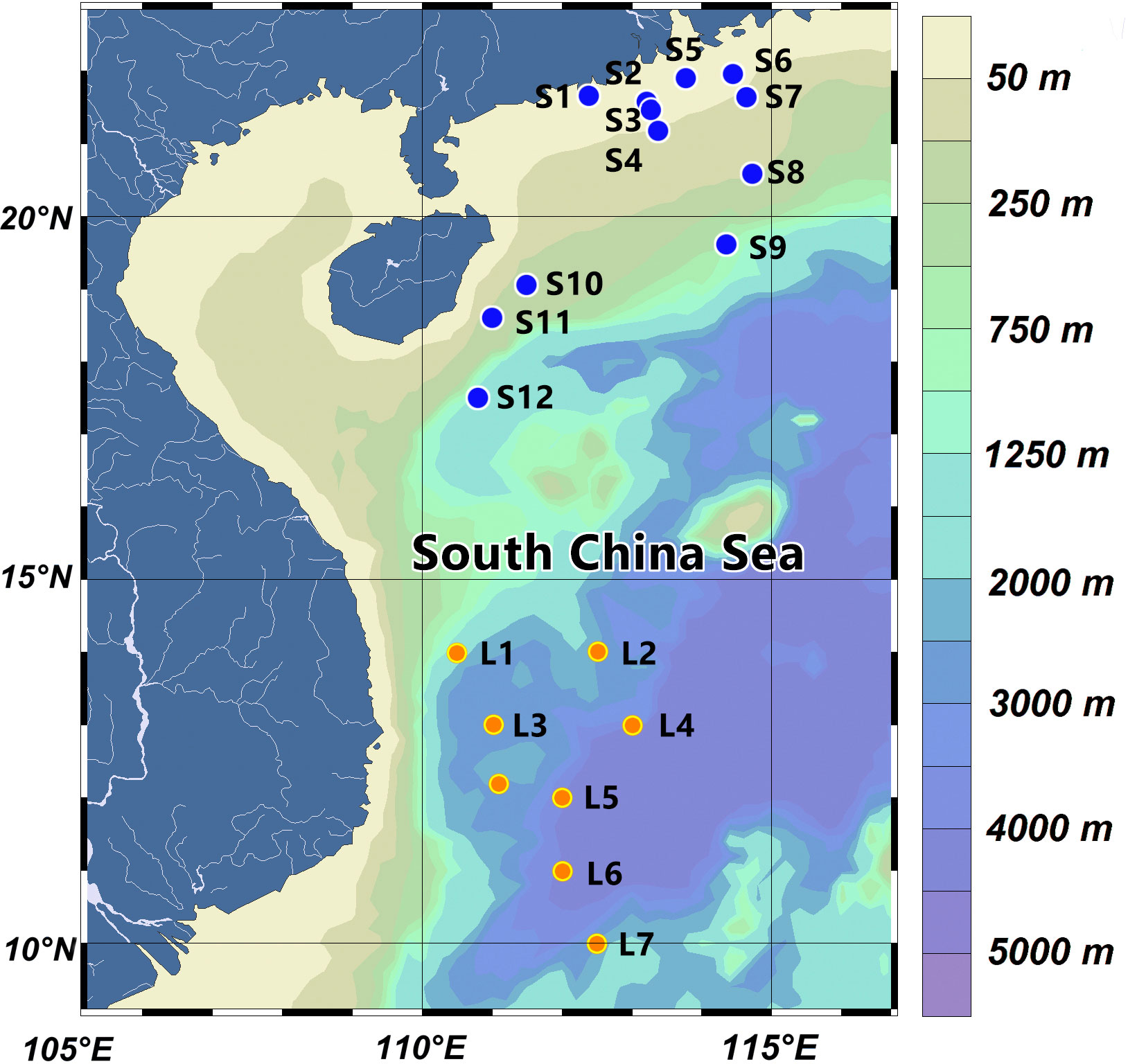
Figure 1 Locations of the 2019 SCS dataset (blue dots) and the 2018 SCS dataset (orange dots).

2.2 In situ sampling

2.2.1 Primary productivity

PP was determined through on-deck incubation at five light penetration depths (100%, 56%, 22%, 7%, and 1% of the surface PAR) at each station (49 samples in the 2019 SCS dataset and 28 samples in the 2018 SCS dataset) (Liao et al., 2021). Seawater samples were obtained using Niskin bottles connected to a conductivity-temperature-depth (CTD) device (Seabird SBE 911) and were obtained in the morning, prefiltered through a 180-µm mesh to eliminate large zooplankton. These samples were then transferred to acid-clean polycarbonate bottles (Nalgene, USA), with two white bottles and one black bottle collected for each layer. After inoculation with 5-μCi of NaH¹⁴CO₃, samples were incubated in duplicate at five light levels and in the dark at in situ temperature (± 2°C) with a water cooler for 6 h. After incubation, the samples were filtered onto 25-mm GF/F filters (Whatman, USA), and all filters were stored at −20°C until analysis. The filters were fumed with HCl for 12 h to eliminate nonfixed ¹⁴C and then immersed in a 5-mL scintillation cocktail (Ultima Gold) in 20-mL scintillation vials. Radioactivity was measured using a Tri-Carb 2810 TR liquid scintillation analyzer (Perkin-Elmer, USA) (Knap et al., 1996). Water samples for dissolved inorganic carbon (DIC) were preserved with HgCl₂ in amber glass bottles and analyzed using an AS-C3 DIC analyzer (Apollo SciTech, USA) with an infrared CO₂ detector (Li-7000) following the procedure outlined by Cai et al. (Cai et al., 2004). PP was then calculated using Equation 1, where CPM_L and CPM_D represent the counts per minute for the white and black vial samples, respectively, CPM_add is the counts per minute for ¹⁴C addition, and T is the incubation time in hours. To harmonize the units of each variable, PP was converted from mg C m^–3h^–1 to mol C m^–3h^–1.

$\begin{array}{ll}\text{PP}=\text{DIC}\times ({\text{CPM}}_{\text{L}}-{\text{CPM}}_{\text{D}})/{\text{CPM}}_{\text{add}}/\text{T}& (1)\end{array}$

2.2.2 Phytoplankton absorption coefficient

To obtain a_ph(λ), samples were filtered onto GF/F filters (Whatman, USA), placed in cell dishes, and stored in liquid nitrogen until the laboratory analysis took place. The absorption spectra of the particles [a_p(λ)] were measured using the quantitative filter-pad technique by the Transmittance mode (i.e., T mode) with a Lambda 650S ultraviolet–visible spectrophotometer at a 1-nm resolution ranging from 350 to 750 nm (Yentsch, 1962). Before the measurement, a clean GF/F filter was soaked in a 0.2-µm seawater filtrate to obtain a blank. After removing the phytoplankton pigments with methanol, the filters were rescanned to obtain the absorption spectra of nonalgal particles [a_d(λ)] (Kishino et al., 1985). The background signal was corrected by subtracting the absorption values at 750 nm from the entire spectrum (Bricaud and Stramski, 1990), and the optical path amplification effect was corrected according to the method of Stramski et al. (Stramski et al., 2015). The obtained difference between a_p(λ) and a_d(λ) was taken to be a_ph(λ).

2.2.3 Phytoplankton pigments

The quantification of pigments was accomplished using high-performance liquid chromatography (HPLC), as outlined by Zapata et al. (Manuel et al., 2000). Following filtration onto Whatman GF/F filters and subsequent storage in liquid nitrogen, samples were subjected to an extraction procedure involving 1.5 ml 95% methanol solution at 4°C for 24 hours. A mixture of 1 ml of extract and 200 µl ultrapure water was then prepared for measurement. A Waters 2695 HPLC system was employed, with signals being detected by a Waters 2998 photodiode array detector. As per the methodology of Zapata et al. (Manuel et al., 2000), pigments containing Chlorophyll a, Chlorophyll b, Chlorophyll c_1,2,3, Divinyl chlorophyll a (DVChl a), Divinyl chlorophyll b, Peridinin, Fucoxanthin, Lutein, Diadinoxanthin, Diatoxanthin, Antheraxanthin, Violaxanthin, Zeaxanthin, Alloxanthin, 19′-hex-fucoxanthin, 19′-but-fucoxanthin, Neoxanthin, and β-carotene were analyzed. Quantification was confirmed by the standards manufactured by the Danish Hydraulic Institute (DHI) Water and Environment, Hørsholm, Denmark. The dominant phytoplankton within each sample was determined through the characteristic pigment approach (Alvain et al., 2005). To facilitate the analysis of the HPLC pigments in this study, a grouping system was employed, wherein the pigments were categorized into Chlorophyll, photosynthetic carotenoids (PSCs), and photoprotective carotenoids (PPCs) (Frank and Cogdell, 1996; Dall'Osto et al., 2007; Roy et al., 2011). Specifically, PPCs were calculated as the sum of Violaxanthin, Diadinoxanthin, Alloxanthin, Zeaxanthin, Lutein, and β-carotene, whereas PSCs were calculated as the sum of Peridinin, 19′-but-fucoxanthin, 19′-hex-fucoxanthin and Fucoxanthin.

2.2.4 PAR and temperature

A Profiler II underwater spectral profiling instrument (Satlantic, Canada) was used to record the downwelling irradiance [E_d(λ,z)] of the water column profile during free-fall, employing a range of wavelengths between 350-800 nm and consisting of 136 channels. The original raw data was calibrated using ProSoft 7.7.1.6 (Satlantic, Canada), while PAR was determined by integrating the E_d(λ,z) within the 400-700 nm wavelength range. Sampling takes place during clear and cloudless conditions between 12:00 and 13:00 every day, in sync with the PP incubation experiment. In Southeast Asia, between 12:00 and 18:00, PAR shows an almost linear decreasing trend (Rundel et al., 2017; Vongcharoen et al., 2018). Simultaneously, the tropical climate characteristics of the South China Sea and the duration of the voyage (5 and 7 days) imply that during these days, the daily sunlight pattern remains relatively consistent, and the daily PAR changes are relatively stable. Thus, we simply made this assumption, PAR was multiplied by 3600 to convert its unit from umol m^–2s^–1 to mol m^–2h^–1. Here, the calculated hourly PAR only characterizes the relative trend of PAR changes, not the actual value of the hourly PAR. Temperature profiles were established via a CTD device (Seabird SBE 911).

2.3 Basic model

The basic model of the a_ph(λ)-based marine PP algorithm can be simply expressed as Equation 2 (Barnes et al., 2014):

$\begin{array}{ll}\text{PP}=\varphi \times a_{ph}({\lambda }_0)\times \text{PAR}& (2)\end{array}$

a_ph(λ₀) represents the phytoplankton absorption coefficient at a particular wavelength (443 nm being the selected wavelength for this study). PAR is photosynthetic active radiation. The quantum yield, represented by $\varphi$ is given by the slope, which denotes the efficiency of photosynthesis in converting absorbed light energy into organic carbon. Under varying physicochemical conditions or in distinct marine areas, $\varphi$ may exhibit fluctuations concerning light intensity, temperature, phytoplankton community structure, and nutrients (Iluz and Dubinsky, 2013; Zoffoli et al., 2018). If Equation 2 proves to be applicable to the 2019 SCS dataset, the regionalization of $\varphi$ in the SCS can be established.

2.4 Statistics

The statistical analyses were conducted using OriginPro (OriginLab Corporation, USA) and Python 3.8.1. A probability coefficient was employed to assess the statistical significance of the correlation between two variables, with a p-value threshold of 0.05. The regression model was evaluated using several statistical metrics, including the adjusted coefficient of determination (Adj.R²) (a penalty can be given for adding nonsignificant variables, i.e., adding an arbitrary variable does not necessarily increase the model fit, and Adj.R² can be positive or negative), the mean square difference (MSD), root mean square difference (RMSD), and the mean absolute difference (MAD). The standard deviation (σ) was used to measure the dispersion of the data, while bias quantified the difference between the observed and predicted values. All non-integer values, except for the p-value were reported to two significant digits. The mathematical expressions for these statistical metrics are provided below:

$\begin{array}{ll}RMSD=\sqrt{\frac{{\sum }_{i=1}^n{(Y_i-y_i)}^2}{n}}& (3)\end{array}$

$\begin{array}{ll}MSD=\frac{{\sum }_{i=1}^n{(Y_i-y_i)}^2}{n}& (4)\end{array}$

$\begin{array}{ll}MAD=\frac{{\sum }_{i=1}^n|y_i-m(y)|}{n}& (5)\end{array}$

$\begin{array}{ll}\sigma =\sqrt{\frac{{\sum }_{i=1}^n{(y_i-m(y))}^2}{n}}& (6)\end{array}$

$\begin{array}{ll}\text{Bias}=y_i-Y_i& (7)\end{array}$

where n is the number of data values, Y_i is the predicted value, y_i is the data value in the set, and m(y) is the average value of the dataset.

2.5 K-fold cross-validation and in situ data validation

K-fold cross-validation was employed to test the generalisability of the model (Geisser, 1975), given that the total number of data points did not exceed 50. This technique is widely utilized to evaluate the overall performance of models (Russell, 2010). Specifically, the dataset was divided into K nearly equal partitions, where K-1 partitions were employed to construct the model, and the remaining sample was used for validation. This process was iterated K times, resulting in K learners, with each fold serving as the validation data (Fushiki, 2011).

The choice of K is an important consideration, as underfitting or overfitting of learners can occur with small or large K values, respectively, which can adversely impact the assessment of general model performance. Although typical K values range between 5 and 10, researchers have suggested other values as well (Jung, 2018). In this study, K values were not arbitrarily chosen, rather, the mean MSD of K learners and the standard deviation of the mean MSD were evaluated over a range of K values, from 2 to 49. With increasing K, the standard deviation of the mean MSD increased, and when K was either less than 10 or greater than 20, the mean MSD exhibited pronounced fluctuations (Figure 2). Therefore, K was set to 10, which resulted in a small standard deviation of the mean MSD and a stable mean MSD across K learners. Accordingly, a 10-fold cross-validation approach was employed in section 3.2.

FIGURE 2

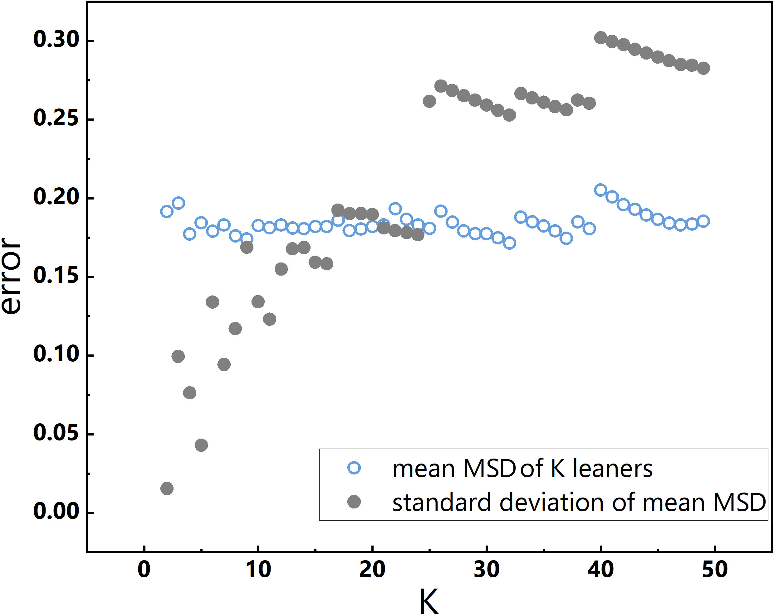
Figure 2 Changes in K and corresponding changes in the mean MSD of K learners and the standard deviation of the mean MSD.

In addition, the 2018 SCS dataset was used to validate the adaptability of the model in the SCS basin waters.

2.6 Sensitivity analysis

The sensitivity of the model was tested using the Monte Carlo method, a widely adopted statistical technique in simulation studies (Brewin et al., 2017). In essence, a normal distribution was generated through Monte Carlo simulation, with either a_ph(443) or PAR serving as the mean value at any given station. To reflect measurement error, we introduced errors of 5% for a_ph(443) and 10% and 20% for PAR, based on empirical measurement estimations. Subsequently, the Monte Carlo method was employed to generate numbers, which were then fed into the model to obtain a new set of data. This new set of data was then verified as normally distributed, and the standard deviation was calculated as the index of uncertainty. In alignment with the methodology of Brewin et al., the minimum number of iterations required to produce a stable estimate of standard deviation was determined to be 200 (Brewin et al., 2017).

3 Results

3.1 Model building

Upon applying Equation 2 to the 2019 SCS dataset, PP was significantly correlated with a_ph(443)×PAR (Adj.R²=0.55, p-value <0.01), Nevertheless, a direct linear regression between a_ph(443)×PAR and PP suffered from heteroscedasticity. In the 2019 SCS dataset, $\varphi$ was not assumed to be a constant value and thus was neither parameterized nor treated as an independent variable. Instead, it was included in the slope (k) of Equation 8.

To raise the accuracy of a predictive model, a logarithmic transformation of PP and a_ph(443)×PAR was conducted. Subsequently, a log-log linear a_ph(λ)-based regression model for PP (hereafter referred to as the ‘log-log linear PP model’) was built (Equation 8):

$\begin{array}{ll}\log (\text{PP})=\text{k}\times \log (a_{ph}(443)\times \text{PAR})+\text{b}& (8)\end{array}$

Figure 3 presents the values of k (slope) and b (intercept) for the log-log linear PP model, which demonstrates a greater aptitude for fitting the data, as indicated by a higher Adj.R². Moreover, the residual plot depicted in Figure 3 confirms homoscedasticity as a defining feature of the model.

FIGURE 3

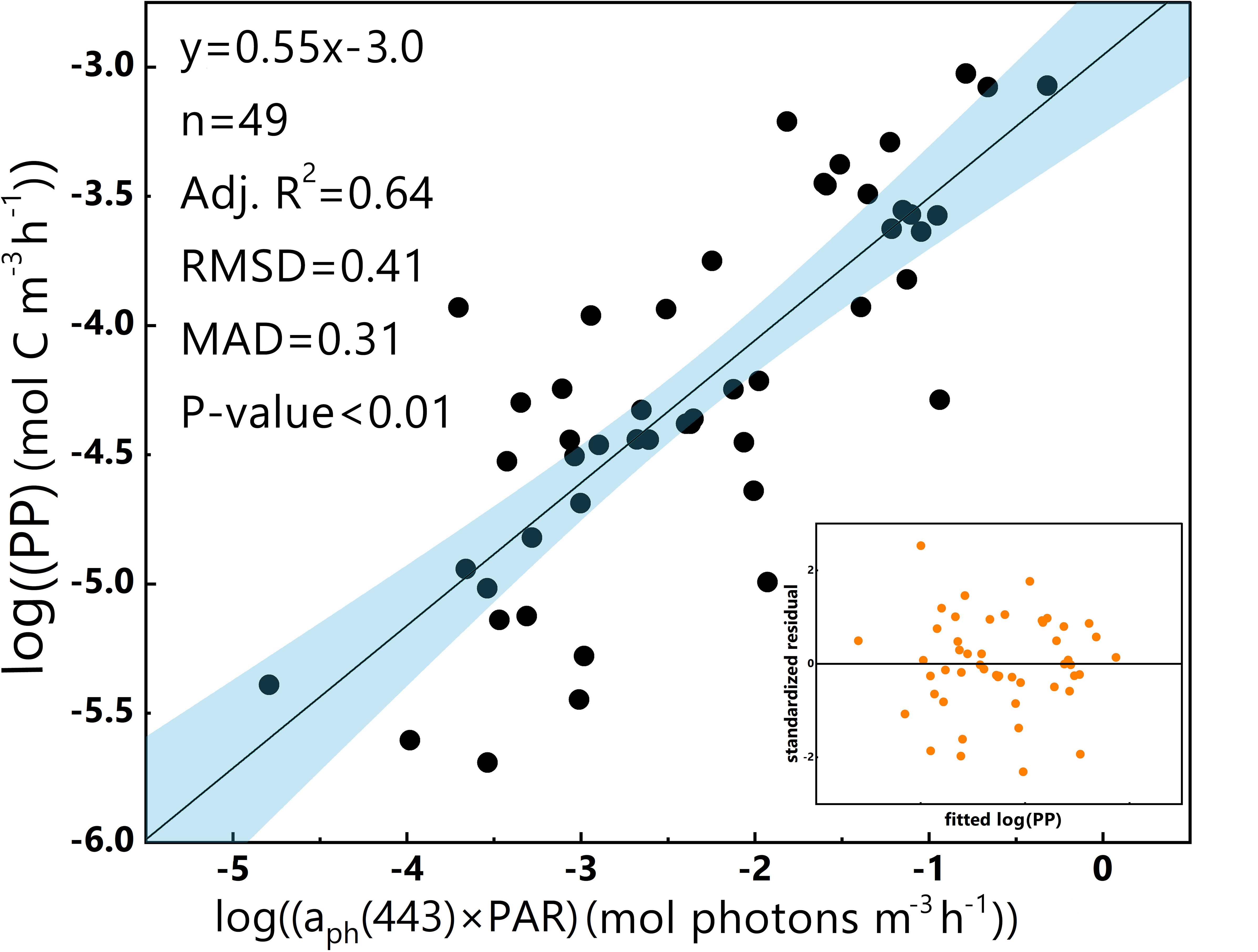
Figure 3 Log-log linear regression of PP and a_ph(443)×PAR in the euphotic zone for the 2019 SCS dataset. The dark line represents the linear regression, and the blue band represents the 95% confidence interval. The residual plot is in the bottom-right corner. The equation, number of data points (n) and some statistical parameters are shown in the upper-left corner.

3.2 K-fold cross-validation and in situ data validation in the log-log linear PP model

At K=10, the standard deviation of the mean MSDs is low (0.13), and the mean MSD derived from cross-validation (0.18) approximates that of the ‘log-log linear PP model’ (0.17). Furthermore, the Adj.R² (0.56) of the relationship between the measured and predicted values derived from cross-validation is quite similar to that of the log-log linear PP model (0.64). Collectively, the results of K-fold cross-validation affirm the commendable generalisation performance of the log-log linear PP model.

An Independent dataset of the SCS in 2018 (2018 SCS dataset, including the in situ a_ph(443), PAR, and PP) was used to verify our model. The logarithmic bias between the predicted and measured PP was approximately 0.077, leading to a deviation of nearly 10% in PP estimates (Figure 4). These results corroborated the model’s robustness and effectiveness for data collected in estuarine, coastal, and offshore areas (2019 SCS dataset) and data collected within the SCS basin (2018 SCS dataset).

FIGURE 4

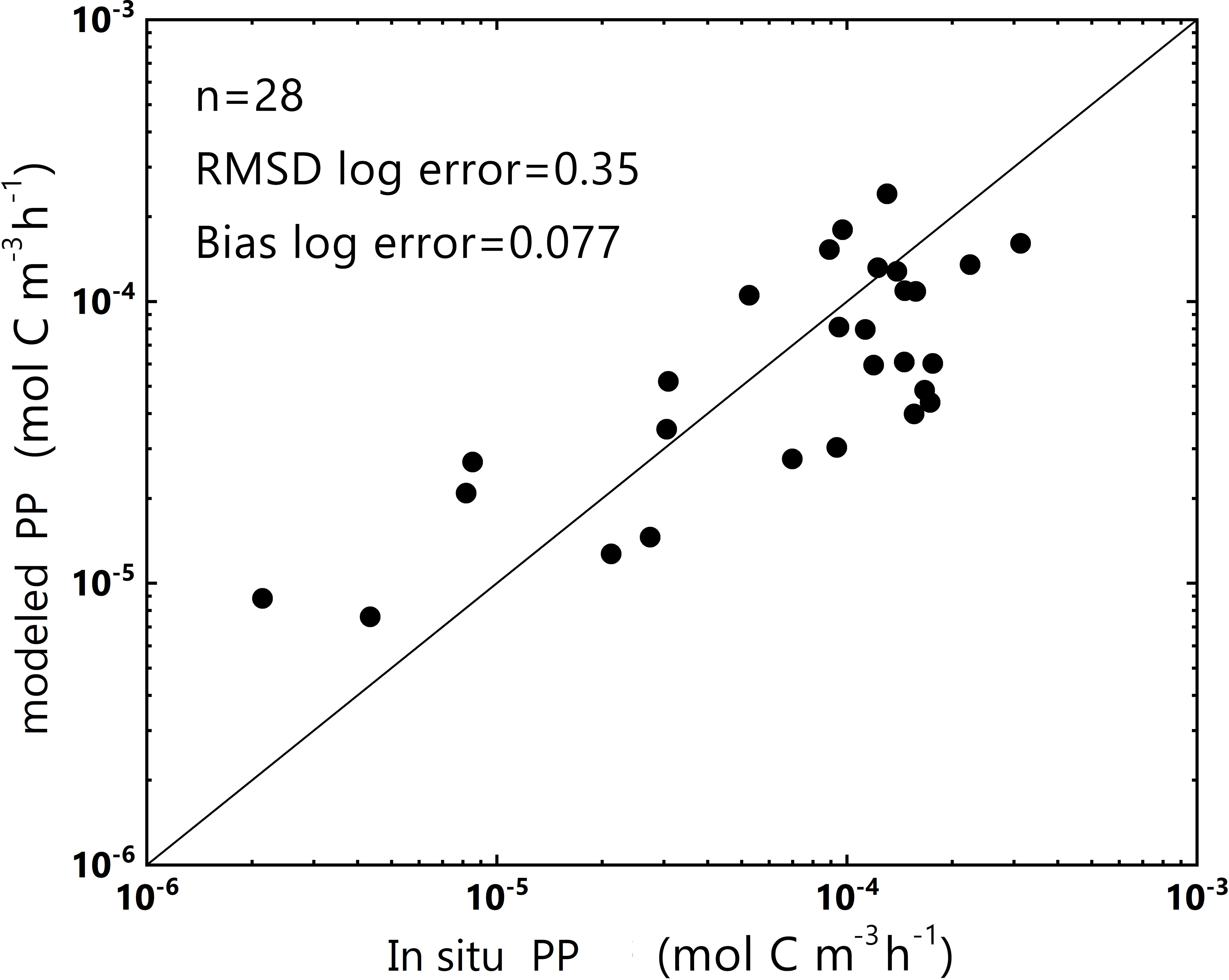
Figure 4 Plot of PP obtained from the log-log linear PP model and in situ PP from the 2018 SCS dataset (in log-scale). y = x is represented by the dark line. The number of data points (n) and some statistical parameters are shown in the upper-left corner.

3.3 Sensitivity analysis of the log-log linear PP model

The inclusion of a 5% standard deviation of a_ph(443) caused a 2.9% standard deviation in the predicted PP (Figure 5). Moreover, the incorporation of 10% and 20% standard deviations of PAR resulted in 5.1% and 11% standard deviations in the predicted PP, respectively. This analysis reveals that the log-log linear PP model is more sensitive to alterations in PAR than to changes in a_ph(443).

FIGURE 5

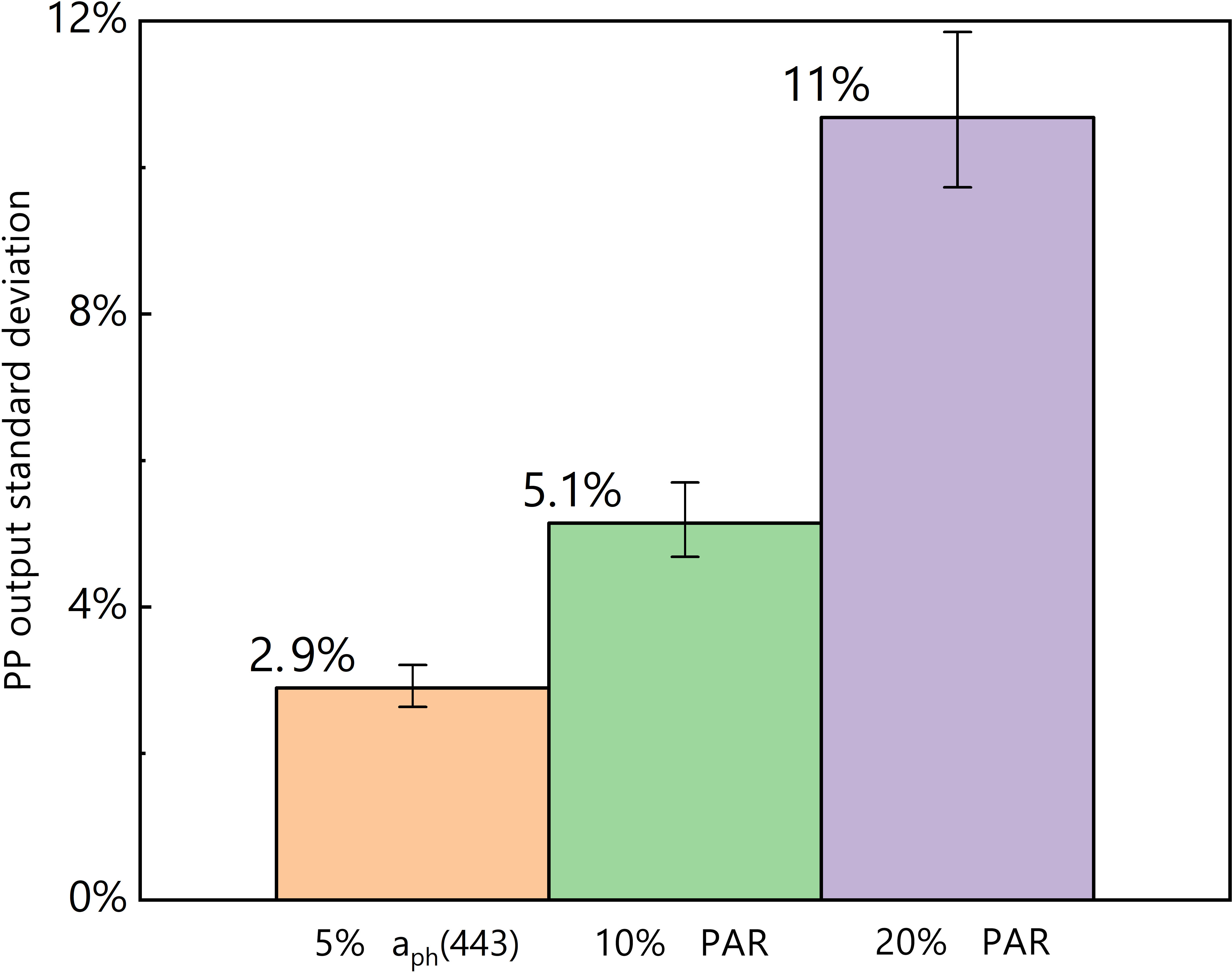
Figure 5 Results of the sensitivity analysis; orange = input of 5% a_ph(443) standard deviation, green = input of 10% PAR standard deviation, and purple = input of 20% PAR standard deviation.

3.4 Identification of dominant phytoplankton clusters

Phytoplankton groups responded differently to environmental variables, such as temperature, light, and nutrient availability, due to their diverse physiological characteristics. Phytoplankton species vary with depths (e.g., sea surface and maximum chlorophyll depth) and marine environments. Therefore, the dominant phytoplankton species were identified to examine their impact on the log-log linear PP model.

Based on the characteristic pigment approach as defined by Alvain et al. (2005), five major phytoplankton species were identified, namely diatoms (Diato), dinoflagellates (Dino), Prochlorococcus (Pro), haptophytes (Hapto), and Synechococcus-like cyanobacteria (SLC) (Figure 6). However, the SLC-dominant and Dino-dominant clusters, consisting of limited sample sizes (only two and five samples, respectively), are not discussed in this study.

FIGURE 6

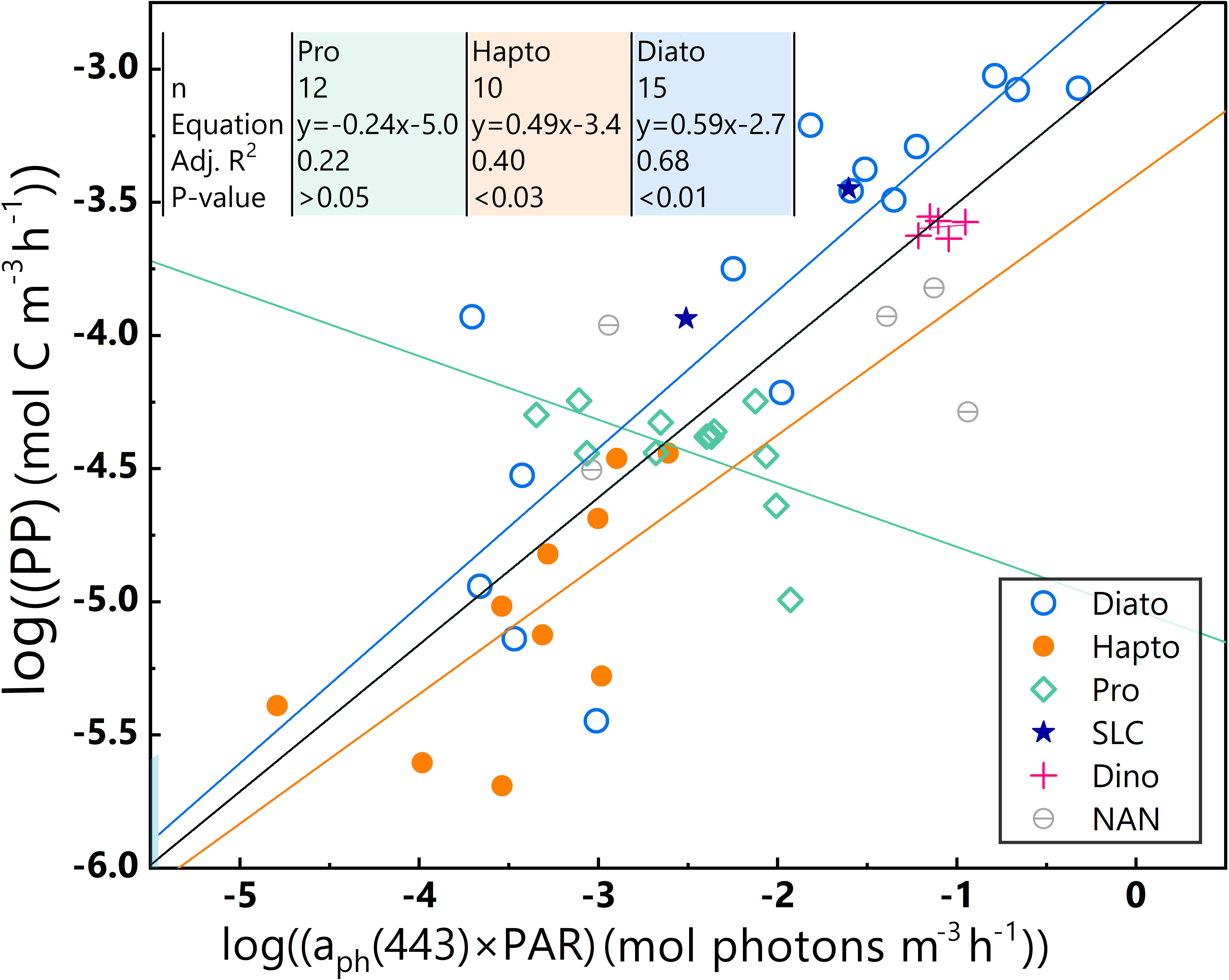
Figure 6 Different dominant phytoplankton samples are represented by various colours and shapes. Log-log linear regressions of PP and a_ph(443)×PAR of the whole dataset and three phytoplankton-dominant clusters in the euphotic zone for the 2019 SCS dataset; black line = whole dataset, blue line = Diato-dominant cluster, orange line = Hapto-dominant cluster, green line = Pro-dominant cluster. Equations, numbers of data points (n), and some statistical parameters of Pro-, Hapto- and Diato-dominant clusters are shown in the upper-left corner.

4 Discussion

4.1 Bio-optical characteristics of different dominant phytoplankton clusters

Table 1 lists statistical results for the varied bio-optical parameters of Diato-, Hapto-, and Pro-dominant phytoplankton clusters, which exhibit differences in their response to environmental variables and physiological characteristics.

TABLE 1

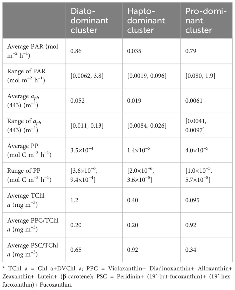
Table 1 Statistical results for the bio-optical parameters of each dominant phytoplankton cluster.

The Diato-dominant cluster has the largest average a_ph(443), average PAR, and average PP values, as well as the largest range of variable variations. In contrast, the Pro-dominant cluster has a smaller average PAR value than the Diato-dominant cluster, but the smallest mean a_ph(443) value and a limited range of variation, especially for PP. The Hapto-dominant cluster presents the lowest average values for PAR and PP, with a mid-range variability. These distinct bio-optical characteristics of the dominant phytoplankton clusters are reflected in their different distribution patterns as seen in Figure 6, which in turn impacts the statistical properties of the log-log linear PP model. To delve deeper into these effects, a linear regression was performed for each cluster in Figure 6.

To identify the photophysiological state of the dominant phytoplankton, we examined their pigment composition. Pigments play a crucial role in phytoplankton photosynthesis. Roy et al. illustrated that phytoplankton can modify their pigment pool which comprises two functional classes: photosynthetic carotenoids (PSCs) and photoprotective carotenoids (PPCs), in response to variable light intensities (Roy et al., 2011). PPCs primarily dissipate excess light energy in the form of heat and to protect photosynthetic organs, while PSCs mainly transmit light energy. According to previous studies (Frank and Cogdell, 1996; Dall'Osto et al., 2007; Roy et al., 2011), the pigments in this study were categorized into Chlorophyll, PPC and PSC and subsequently normalized to TChl a (Table 1).

4.2 Pro-dominant cluster

Figure 6 displays a negative fitting slope for the Pro-dominant cluster, which contrasts with the fitting slope of the whole dataset. To understand this phenomenon, we examined the relationships of a_ph(443) with PP (in order to estimate the impact of biomass on PP) and PAR with PP/TChl a (in order to estimate the impact of PAR on PP. Additionally, to eliminate the impact of biomass on PP, PP was normalized to TChl a) (Figure 7).

FIGURE 7

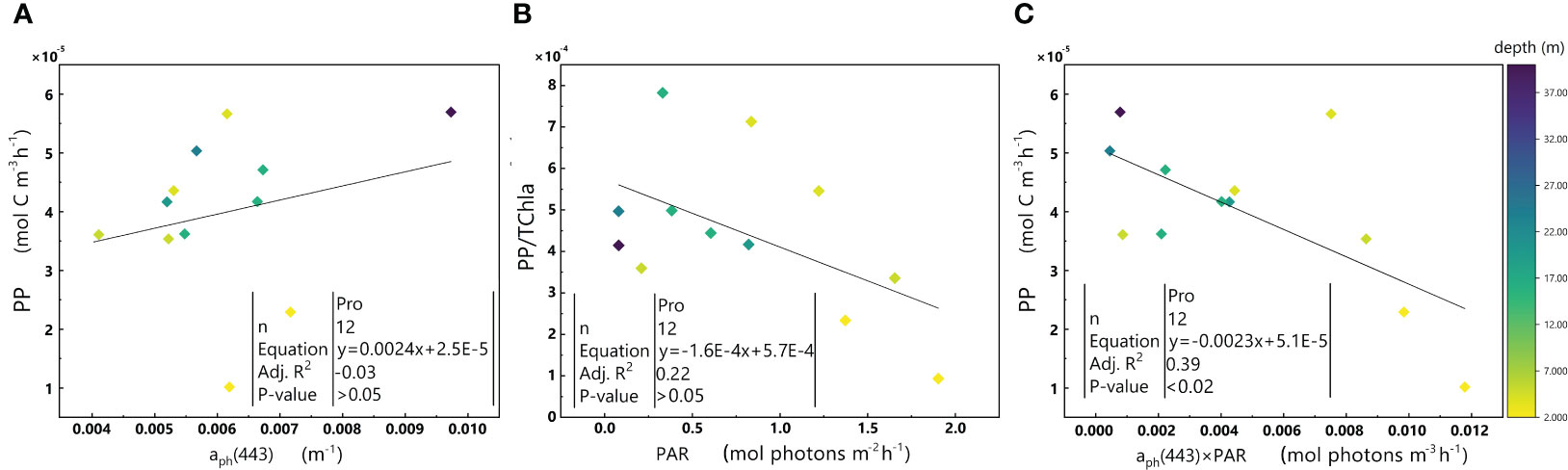
Figure 7 Relationships between a_ph(443) and PP (A), PAR and PP/TChl a (B), and a_ph(443)×PAR and PP (C) in the euphotic zone for the Pro-dominant cluster in the 2019 SCS dataset. Colorbar represents depth. Equations and some statistical parameters are also shown.

a_ph(443) does not exhibit a significant relationship with PP (p-value > 0.05) in Figure 7A. However, the ratio of PP/TChl a decreases with an increase in PAR (Figure 7B), which is comparable to the relationship between a_ph(443)×PAR and PP (Figure 7C).

The Pro-dominant cluster has a significantly higher PPC/TChl a and a much lower PSC/TChl a than the other two clusters (Table 1), Since most of the samples within the Pro-dominant cluster results from the surface and in the upper layer (shallower than the maximum chlorophyll a layer), the negative correlation between PAR and PP/TChl a in the Pro-dominant cluster may be attributed to the photoinhibition of phytoplankton.

For Prochlorococcus photosynthesis, Hess et al. suggested that the optimum irradiance is 200 μmol photons m^–2 s^–1 for the surface and 30–50 μmol photons m^–2 s^–1 for deeper water, respectively (Hess et al., 2001). However, all of the PAR values in our dataset are beyond the suggested optimum irradiance for both at the sea surface and deeper water. Additionally, temperatures in waters with the Pro-dominant cluster were high (28–29°C). The photoinhibition of Prochlorococcus is generally more pronounced in high temperature than in low temperature ranges at the same irradiance (Xiao et al., 2019).

Ultraviolet light and high light intensity increase the production of reactive oxygen species, which damages the PSII reaction centre and antenna complexes (Dring et al., 2001; Van De Poll et al., 2001; He and Häder, 2002; Sarvikas et al., 2006; Rastogi et al., 2010; Mella-Flores et al., 2012). PPC/TChl a in the Pro-dominant cluster does not exhibit an obvious upward trend with increasing PAR (Figure 8) likely since that Prochlorococcus has a limited mechanism for nonphotochemical quenching (NPQ) (Rocap et al., 2003; Xu et al., 2017; Xu et al., 2018). Moreover, the PSII repair capacity of Prochlorococcus reaches a maximum of approximately 400 μmol photons m^–2 s^–1 (Mella-Flores et al., 2012). Thus, it appears that the Pro-dominant cluster, when exposed to high light intensity, has a constrained ability for self-protection and self-repair, making it more susceptible to photoinhibition.

FIGURE 8

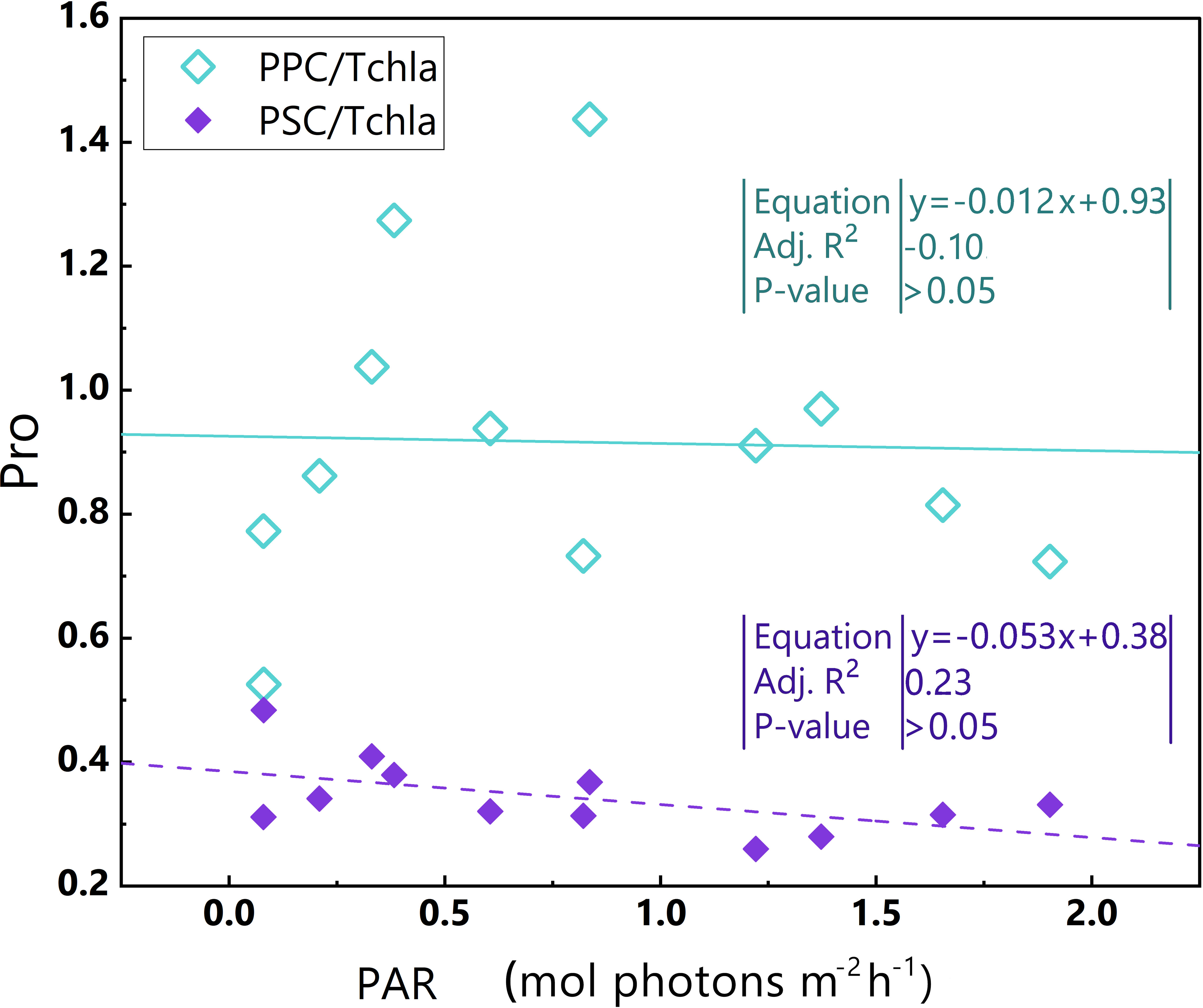
Figure 8 Relationships between PAR and PPC/TChl a, PAR and PSC/TChl a in the euphotic zone for the Pro-dominant cluster in the 2019 SCS dataset. Linear regression for PAR and PSC/TChl a (purple dotted line) and linear regression for PAR and PPC/TChl a (green line). Equations and some statistical parameters are also shown (green text for green line, purple text for purple dotted line).

During photoinhibition, both the quantum efficiency ($\varphi$) and the maximum photosynthetic efficiency decrease (Cullen and Renger, 1979; Powles, 1984; Lesser et al., 1994; Behrenfeld et al., 1998; Marshall et al., 2000; Andersson and Aro, 2001; Oliver et al., 2003; Ross et al., 2008). As a consequence, PP values also diminish.

4.3 Hapto-dominant cluster and Diato-dominant cluster

The significant positive correlations between a_ph(443) ×PAR and PP were observed in both Hapto-dominant cluster (Figure 9C) and Diato-dominant cluster (Figure 10C).

FIGURE 9

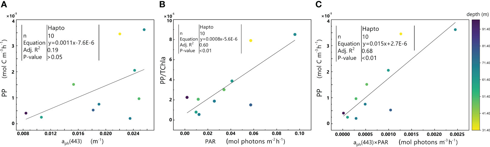
Figure 9 Relationships between a_ph(443) and PP (A), PAR and PP/TChl a (B), and a_ph(443)×PAR and PP (C) in the euphotic zone for the Hapto-dominant cluster in the 2019 SCS dataset. Colorbar represents depth. Equations and some statistical parameters are also shown.

FIGURE 10

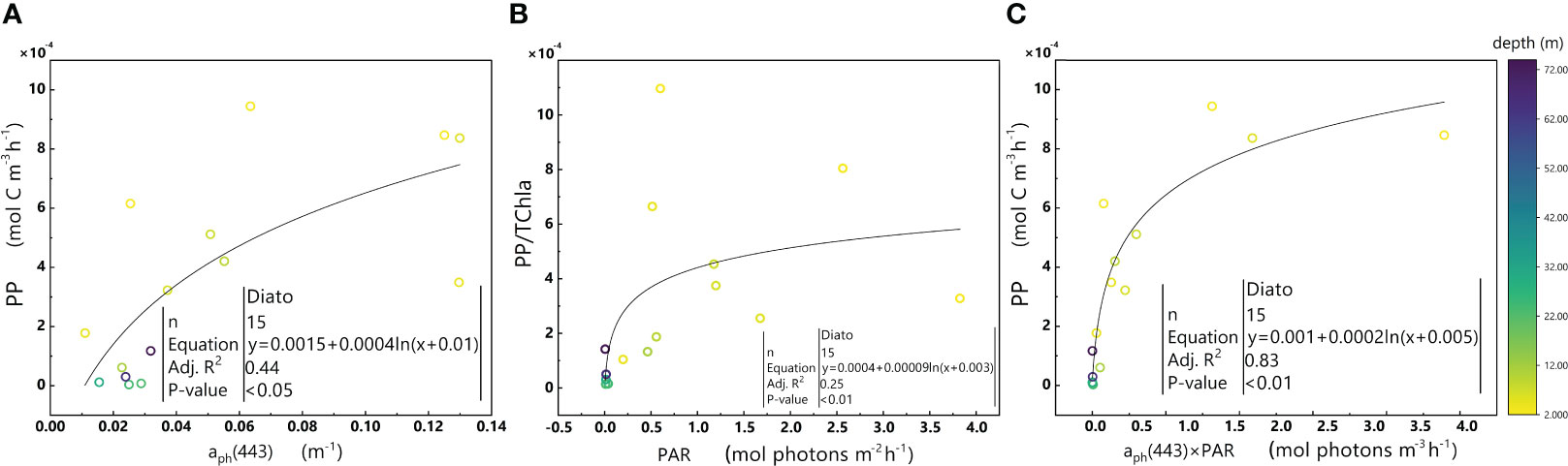
Figure 10 Relationships between a_ph(443) and PP (A), PAR and PP/TChl a (B), and a_ph(443)×PAR and PP (C) in the euphotic zone for the Diato-dominant cluster in the 2019 SCS dataset. Colorbar represents depth. Equations and some statistical parameters are also shown.

In addition, no significant relationship exists between a_ph(443) and PP (p-value>0.05) (Figure 9A), while there is a significant positive correlation between PAR and PP/TChl a (Figure 9B), similar to the trend observed between a_ph(443) ×PAR and PP (Figure 9C). These results implied that PAR plays a pivotal role in regulating PP in this cluster. Interestingly, the Hapto-dominant cluster exhibits a considerably higher level of PSC/TChl a than the other two clusters (Table 1), indicating that phytoplankton in the Hapto-dominant cluster may be light-limited. This suggestion is in agreement with the observation that phytoplankton in this cluster inhabit deeper regions with low light intensity beneath the mixed layer. Therefore, the higher PSC/TChl a ratio in the Hapto-dominant cluster may be an adaptive strategy to enhance its light absorption and utilization under conditions of limited light availability.

The Diato-dominant cluster displays positive covariance between a_ph(443) and PP (Figure 10A), as well as between PAR and PP/TChl a (Figure 10B). These relationships are consistent with the significant correlation observed between a_ph(443) ×PAR and PP (Figure 10C).

Phytoplankton within the Diato-dominant cluster mainly appeared at both the surface and in deeper water layers in coastal and estuarine areas. The level of the PPC/TChl a of the Diato-dominant cluster is similar to that of the Hapto-dominant cluster, but higher than that of PSC/TChl a. It is reasonable to infer that most samples in the Diato-dominant cluster are also in a light-limited stage, with several diatom-dominated samples appearing to be light-saturated. Remarkably, despite some samples in the Diato-dominant cluster being subjected to much stronger light intensities than those in the Pro-dominant cluster, photoinhibition does not occur in this cluster. Unlike the Pro-dominant cluster, the PPC/TChla of the Diato-dominant cluster increases significantly with the enhancement of light intensity (Figure 11), which likely protects it from the damage caused by photoinhibition. Furthermore, the mechanism of small photoregulation movements, the xanthophyll cycle and non-photochemical quenching (NPQ) may also safeguard diatoms from high light intensity to some extent (Prins et al., 2020).

FIGURE 11

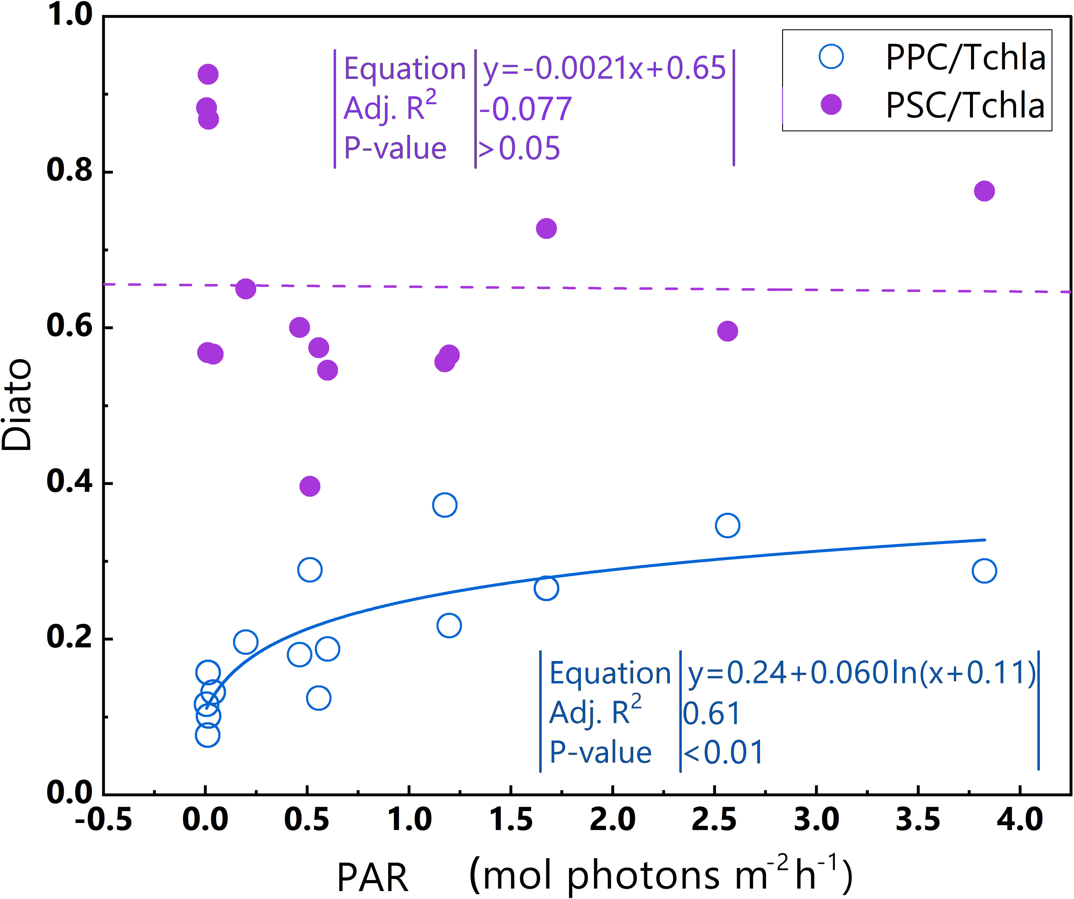
Figure 11 Relationships between PAR and PPC/TChl a and between PAR and PSC/TChl a in the euphotic zone for the Diato-dominant cluster in the 2019 SCS dataset. Linear regression for PAR and PSC/TChl a (purple dotted line) and log regression for PAR and PPC/TChl a (blue line). Equations and some statistical parameters are also shown (blue text for blue line, purple text for purple dotted line).

5 Conclusions

A log-log linear primary production (PP) model based on the regional phytoplankton absorption coefficient [a_ph(λ)] was developed for the South China Sea (SCS), using an in situ dataset complied from the observation data collected in 2019. The predictive capacity of the model was evaluated by statistical analysis, K-fold cross validation, and in situ data validation, indicating that it can well predict PP across marine environment, ranging from estuarine to offshore and basin. The model’s response is more sensitive to changes in photosynthetically active radiation (PAR) than to changes in a_ph(443).

To account for the bio-optical characteristics of different dominant phytoplankton in the SCS, the dataset was divided into five dominant phytoplankton clusters. The study analyzed the effects of environmental variables and physiological characteristics on the log-log linear PP model for the Diato-dominant, Hapto-dominant, and Pro-dominant clusters. The Diato-dominant and the Hapto-dominant clusters are mostly in the light-limited stage. Although some samples in the Diato-dominant clusters were exposed to extremely high light intensity, diatoms have efficient pigment regulation mechanisms and other ways to adapt to high light intensity. The Hapto-dominant cluster appeared below the mixed layer, where light is undersaturation. As a result, an increase in light levels, as indicated by a_ph(443)×PAR, leads to a corresponding increase in PP for both clusters. In contrast, the Pro-dominant cluster exhibited an opposite trend, suggesting that this cluster undergoes photoinhibition due to samples exposure to extremely high light intensity and the lack of self-protection mechanism.

Therefore, the accuracy of the log-log linear PP model depends on the photo-physiological state of the phytoplankton. In natural marine environment, dominant phytoplankton assemblages may be in different physiological states, varying from light inhibition to light limitation simultaneously. Large-scale photoinhibition may lead to inaccurate PP predictions. However, if phytoplankton are light-limited, the log-log linear PP model can well predict PP. Our findings provide insights into the establishment of phytoplankton-specific primary productivity models in marine environments.

Data availability statement

The datasets presented in this study can be found in online repositories. The names of the repository/repositories and accession number(s) can be found below: https://doi.org/10.5281/zenodo.5709178.

Author contributions

Conceptualization, HZ and WZ. Methodology, HZ, WC, JL, WDZ, WZ, and YZ. Software, HZ and KZ. Validation, HZ, WZ, and WC. Formal Analysis, HZ. Investigation, JL, LD, and KZ. Resources, WZ, WC, and JX. Data Curation, HZ. Writing – Original Draft Preparation, HZ. Writing – Review & Editing, HZ, WZ, WC, KZ, JX, and LD. Visualization, HZ. Supervision, WZ and WC. Project Administration, WZ and WC. Funding Acquisition, WZ and WC. All authors contributed to the article and approved the submitted version.

Funding

The author(s) declare financial support was received for the research, authorship, and/or publication of this article. Financial support for this research was provided by Science & Technology Fundamental Resources Investigation Program (Grant No.2022FY100601); National Natural Science Foundation of China (NSFC) (41976170, 42276181, 41976172, 41976181); Guangdong Basic and Applied Basic Research Foundation (2023A1515011703).

Acknowledgments

The authors would like to thank the co-workers and researchers of R/V Haike 68 and R/V Shiyan 3 supported by NSFC Shiptime Sharing Project. In addition, we would like to thank Dr. Xin Liu for conducting HPLC-CHEMTAX validation work on the classification of dominant phytoplankton clusters.

Conflict of interest

The authors declare that the research was conducted in the absence of any commercial or financial relationships that could be construed as a potential conflict of interest.

Publisher’s note

All claims expressed in this article are solely those of the authors and do not necessarily represent those of their affiliated organizations, or those of the publisher, the editors and the reviewers. Any product that may be evaluated in this article, or claim that may be made by its manufacturer, is not guaranteed or endorsed by the publisher.

References

Aiken J., Hardman-Mountford N. J., Barlow R., Fishwick J., Hirata T., Smyth T. (2008). Functional links between bioenergetics and bio-optical traits of phytoplankton taxonomic groups: an overarching hypothesis with applications for ocean colour remote sensing. J. Plankton Res. 30 (2), 165–181. doi: 10.1093/plankt/fbm098

CrossRef Full Text | Google Scholar

Alvain S., Moulin C., Dandonneau Y., Bréon F. M. (2005). Remote sensing of phytoplankton groups in case 1 waters from global SeaWiFS imagery. Deep Sea Res. Part I: Oceanogr. Res. Papers 52 (11), 1989–2004. doi: 10.1016/j.dsr.2005.06.015

CrossRef Full Text | Google Scholar

Andersson B., Aro E.-M. (2001). “Photodamage and D1 protein turnover in photosystem II,” in Regulation of Photosynthesis. Eds. Aro E.-M., Andersson B. (Dordrecht: Springer Netherlands), 377–393.

Google Scholar

Antoine D., Morel A. (1996). Oceanic primary production: 1. Adaptation of a spectral light-photosynthesis model in view of application to satellite chlorophyll observations. Global Biogeochem. Cycles 10 (1), 43–55. doi: 10.1029/95GB02831

CrossRef Full Text | Google Scholar

Barnes M. K., Tilstone G. H., Smyth T. J., Suggett D. J., Astoreca R., Lancelot C., et al. (2014). Absorption-based algorithm of primary production for total and size-fractionated phytoplankton in coastal waters. Mar. Ecol. Prog. Ser. 504, 73–89. doi: 10.3354/meps10751

CrossRef Full Text | Google Scholar

Behrenfeld M. J., Prasil O., Kolber Z. S., Babin M., Falkowski P. G. (1998). Compensatory changes in Photosystem II electron turnover rates protect photosynthesis from photoinhibition. Photosynth. Res. 58 (3), 259–268. doi: 10.1023/A:1006138630573

CrossRef Full Text | Google Scholar

Boyce D. G., Lewis M. R., Worm B. (2010). Global phytoplankton decline over the past century. Nature 466 (7306), 591–596. doi: 10.1038/nature09268

PubMed Abstract | CrossRef Full Text | Google Scholar

Brewin R. J. W., Morán X. A. G., Raitsos D. E., Gittings J. A., Calleja M. L., Viegas M., et al. (2019). Factors regulating the relationship between total and size-fractionated chlorophyll-a in coastal waters of the Red Sea. Front. Microbiol. 10. doi: 10.3389/fmicb.2019.01964

CrossRef Full Text | Google Scholar

Brewin R. J. W., Tilstone G. H., Jackson T., Cain T., Miller P. I., Lange P. K., et al. (2017). Modelling size-fractionated primary production in the Atlantic Ocean from remote sensing. Prog. Oceanogr. 158, 130–149. doi: 10.1016/j.pocean.2017.02.002

CrossRef Full Text | Google Scholar

Bricaud A., Claustre H., Ras J., Oubelkheir K. (2004). Natural variability of phytoplanktonic absorption in oceanic waters: Influence of the size structure of algal populations. J. Geophys. Res.: Oceans 109 (C11). doi: 10.1029/2004JC002419

CrossRef Full Text | Google Scholar

Bricaud A., Stramski D. (1990). Spectral absorption coefficients of living phytoplankton and nonalgal biogenous matter: A comparison between the Peru upwelling areaand the Sargasso Sea. Limnol. Oceanogr. 35 (3), 562–582. doi: 10.4319/lo.1990.35.3.0562

CrossRef Full Text | Google Scholar

Cai W.-J., Dai M., Wang Y., Zhai W., Huang T., Chen S., et al. (2004). The biogeochemistry of inorganic carbon and nutrients in the Pearl River estuary and the adjacent Northern South China Sea. Cont. Shelf Res. 24 (12), 1301–1319. doi: 10.1016/j.csr.2004.04.005

CrossRef Full Text | Google Scholar

Campbell J., Antoine D., Armstrong R., Arrigo K., Balch W., Barber R., et al. (2002). Comparison of algorithms for estimating ocean primary production from surface chlorophyll, temperature, and irradiance. Global Biogeochem. Cycles 16 (3), 9–1-9-15. doi: 10.1029/2001GB001444

CrossRef Full Text | Google Scholar

Ciotti Á. M., Lewis M. R., Cullen J. J. (2002). Assessment of the relationships between dominant cell size in natural phytoplankton communities and the spectral shape of the absorption coefficient. Limnol. Oceanogr. 47 (2), 404–417. doi: 10.4319/lo.2002.47.2.0404

CrossRef Full Text | Google Scholar

Claustre H., Babin M., Merien D., Ras J., Prieur L., Dallot S., et al. (2005). Toward a taxon-specific parameterization of bio-optical models of primary production: A case study in the North Atlantic. J. Geophys. Res.: Oceans 110 (C7). doi: 10.1029/2004JC002634

CrossRef Full Text | Google Scholar

Cloern J. E., Foster S., Kleckner A. (2014). Phytoplankton primary production in the world's estuarine-coastal ecosystems. Biogeosciences 11 (9), 2477–2501. doi: 10.5194/bg-11-2477-2014

CrossRef Full Text | Google Scholar

Cullen J. J., Renger E. H. (1979). Continuous measurement of the DCMU-induced fluorescence response of natural phytoplankton populations. Mar. Biol. 53 (1), 13–20. doi: 10.1007/BF00386524

CrossRef Full Text | Google Scholar

Curran K., Brewin R. J. W., Tilstone G. H., Bouman H. A., Hickman A. (2018). Estimation of size-fractionated primary production from satellite ocean colour in UK shelf seas. Remote Sens. 10 (9). doi: 10.3390/rs10091389

CrossRef Full Text | Google Scholar

Dall'Osto L., Cazzaniga S., North H., Marion-Poll A., Bassi R. (2007). The Arabidopsis aba4-1 Mutant Reveals a Specific Function for Neoxanthin in Protection against Photooxidative Stress. Plant Cell 19 (3), 1048–1064. doi: 10.1105/tpc.106.049114

PubMed Abstract | CrossRef Full Text | Google Scholar

Dring M. J., Wagner A., Lüning K. (2001). Contribution of the UV component of natural sunlight to photoinhibition of photosynthesis in six species of subtidal brown and red seaweeds. Plant Cell Environ. 24 (11), 1153–1164. doi: 10.1046/j.1365-3040.2001.00765.x

CrossRef Full Text | Google Scholar

Eppley R. W., Stewart E., Abbott M. R., Heyman U. (1985). Estimating ocean primary production from satellite chlorophyll. Introduction to regional differences and statistics for the Southern California Bight. J. Plankton Res. 7 (1), 57–70. doi: 10.1093/plankt/7.1.57

CrossRef Full Text | Google Scholar

Falkowski P. G., Barber R. T., Smetacek V. (1998). Biogeochemical controls and feedbacks on ocean primary production. Science 281 (5374), 200–206. doi: 10.1126/science.281.5374.200

PubMed Abstract | CrossRef Full Text | Google Scholar

Frank H. A., Cogdell R. J. (1996). Carotenoids in photosynthesis. Photochem. Photobiol. 63 (3), 257–264. doi: 10.1111/j.1751-1097.1996.tb03022.x

PubMed Abstract | CrossRef Full Text | Google Scholar

Fushiki T. (2011). Estimation of prediction error by using K-fold cross-validation. Stat. Comput. 21 (2), 137–146. doi: 10.1007/s11222-009-9153-8

CrossRef Full Text | Google Scholar

Geisser S. (1975). The predictive sample reuse method with applications. J. Am. Stat. Assoc. 70 (350), 320–328. doi: 10.1080/01621459.1975.10479865

CrossRef Full Text | Google Scholar

He Y.-Y., Häder D.-P. (2002). Reactive oxygen species and UV-B: effect on cyanobacteria. Photochem. Photobiol. Sci. 1 (10), 729–736. doi: 10.1039/B110365M

PubMed Abstract | CrossRef Full Text | Google Scholar

Hemsley V. S., Smyth T. J., Martin A. P., Frajka-Williams E., Thompson A. F., Damerell G., et al. (2015). Estimating oceanic primary production using vertical irradiance and chlorophyll profiles from ocean gliders in the North Atlantic. Environ. Sci. Technol. 49 (19), 11612–11621. doi: 10.1021/acs.est.5b00608

PubMed Abstract | CrossRef Full Text | Google Scholar

Hess W. R., Rocap G., Ting C. S., Larimer F., Stilwagen S., Lamerdin J., et al. (2001). The photosynthetic apparatus of Prochlorococcus: Insights through comparative genomics. Photosynth. Res. 70 (1), 53–71. doi: 10.1023/A:1013835924610

PubMed Abstract | CrossRef Full Text | Google Scholar

Hilker T., Coops N. C., Wulder M. A., Black T. A., Guy R. D. (2008). The use of remote sensing in light use efficiency based models of gross primary production: A review of current status and future requirements. Sci. Total Environ. 404 (2), 411–423. doi: 10.1016/j.scitotenv.2007.11.007

PubMed Abstract | CrossRef Full Text | Google Scholar

Hirata T., Hardman-Mountford N. J., Barlow R., Lamont T., Brewin R., Smyth T., et al. (2009). An inherent optical property approach to the estimation of size-specific photosynthetic rates in eastern boundary upwelling zones from satellite ocean colour: An initial assessment. Prog. Oceanogr. 83 (1), 393–397. doi: 10.1016/j.pocean.2009.07.019

CrossRef Full Text | Google Scholar

Hirawake T., Takao S., Horimoto N., Ishimaru T., Yamaguchi Y., Fukuchi M. (2011). A phytoplankton absorption-based primary productivity model for remote sensing in the Southern Ocean. Polar Biol. 34 (2), 291–302. doi: 10.1007/s00300-010-0949-y

CrossRef Full Text | Google Scholar

Huot Y., Babin M., Bruyant F., Grob C., Twardowski M. S., Claustre H. (2007). Relationship between photosynthetic parameters and different proxies of phytoplankton biomass in the subtropical ocean. Biogeosciences 4 (5), 853–868. doi: 10.5194/bg-4-853-2007

CrossRef Full Text | Google Scholar

Iluz D., Dubinsky Z. (2013). “Quantum yields in aquatic photosynthesis,” in Photosynthesis (Intech Rijeka), 135–158.

Google Scholar

Jochem F. J., Mathot S., Quéguiner B. (1995). Size-fractionated primary production in the open Southern Ocean in austral spring. Polar Biol. 15 (6), 381–392. doi: 10.1007/BF00239714

CrossRef Full Text | Google Scholar

Jung Y. (2018). Multiple predicting K-fold cross-validation for model selection. J. Nonparametric Stat. 30 (1), 197–215. doi: 10.1080/10485252.2017.1404598

CrossRef Full Text | Google Scholar

Kahru M. (2017). Ocean productivity from space: Commentary. Global Biogeochem. Cycles 31 (1), 214–216. doi: 10.1002/2016GB005582

CrossRef Full Text | Google Scholar

Kameda T., Ishizaka J. (2005). Size-fractionated primary production estimated by a two-phytoplankton community model applicable to ocean color remote sensing. J. Oceanogr. 61 (4), 663–672. doi: 10.1007/s10872-005-0074-7

CrossRef Full Text | Google Scholar

Kiefer D. A., Mitchell B. G. (1983). A simple, steady state description of phytoplankton growth based on absorption cross section and quantum efficiency1. Limnol. Oceanogr. 28 (4), 770–776. doi: 10.4319/lo.1983.28.4.0770

CrossRef Full Text | Google Scholar

Kishino M., Takahashi M., Okami N., Ichimura S. (1985). Estimation of the spectral absorption coefficients of phytoplankton in the sea. Bull. Mar. Sci. 37 (2), 634–642.

Google Scholar

Knap A., Michaels A., Close A., Ducklow H., Dickson A. (1996). Protocols for the joint global ocean flux study (JGOFS) core measurements. JGOFS Reprint IOC Manuals Guides No. 29 UNESCO 1994 19, 111–115. doi: 10.013/epic.27912

CrossRef Full Text | Google Scholar

Lee Z., Carder K. L., Arnone R. A. (2002). Deriving inherent optical properties from water color: a multiband quasi-analytical algorithm for optically deep waters. Appl. Optics 41 (27), 5755–5772. doi: 10.1364/AO.41.005755

CrossRef Full Text | Google Scholar

Lee Z. P., Carder K. L., Marra J., Steward R. G., Perry M. J. (1996). Estimating primary production at depth from remote sensing. Appl. Optics 35 (3), 463–474. doi: 10.1364/AO.35.000463

CrossRef Full Text | Google Scholar

Lesser M. P., Cullen J. J., Neale P. J. (1994). Carbon uptake in A marine diatom during acute exposure to ultraviolet B radiation: relative importance of damage and repair1. J. Phycol. 30 (2), 183–192. doi: 10.1111/j.0022-3646.1994.00183.x

CrossRef Full Text | Google Scholar

Liao J., Xu J., Li R., Shi Z. (2021). Photosynthesis-irradiance response in the eddy dipole in the Western South China sea. J. Geophys. Res.: Oceans 126 (5), e2020JC016986. doi: 10.1029/2020JC016986

CrossRef Full Text | Google Scholar

Manuel Z., Rodríguez F., José L. G. (2000). Separation of chlorophylls and carotenoids from marine phytoplankton: a new HPLC method using a reversed phase C8 column and pyridine-containing mobile phases. Mar. Ecol. Prog. Ser. 195, 29–45. doi: 10.3354/meps195029

CrossRef Full Text | Google Scholar

Marra J., Trees C. C., O’Reilly J. E. (2007). Phytoplankton pigment absorption: A strong predictor of primary productivity in the surface ocean. Deep Sea Res. Part I: Oceanogr. Res. Papers 54 (2), 155–163. doi: 10.1016/j.dsr.2006.12.001

CrossRef Full Text | Google Scholar

Marshall H. L., Geider R. J., Flynn K. J. (2000). A mechanistic model of photoinhibition. New Phytol. 145 (2), 347–359. doi: 10.1046/j.1469-8137.2000.00575.x

CrossRef Full Text | Google Scholar

Mella-Flores D., Six C., Ratin M., Partensky F., Boutte C., Le Corguillé G., et al. (2012). Prochlorococcus and synechococcus have evolved different adaptive mechanisms to cope with light and UV stress. Front. Microbiol. 3. doi: 10.3389/fmicb.2012.00285

PubMed Abstract | CrossRef Full Text | Google Scholar

Moore T. S., Campbell J. W., Dowell M. D. (2009). A class-based approach to characterizing and mapping the uncertainty of the MODIS ocean chlorophyll product. Remote Sens. Environ. 113 (11), 2424–2430. doi: 10.1016/j.rse.2009.07.016

CrossRef Full Text | Google Scholar

Morel A., Maritorena S. (2001). Bio-optical properties of oceanic waters: A reappraisal. J. Geophys. Res.: Oceans 106 (C4), 7163–7180. doi: 10.1029/2000JC000319

CrossRef Full Text | Google Scholar

Nielsen E. S. (1952). Use of radio-active carbon (/sup 14/C) for measuring organic production in the sea. ICES J. Mar. Sci. 18, 2. doi: 10.1093/icesjms/18.2.117

CrossRef Full Text | Google Scholar

Oliver M. J., Schofield O., Bergmann T., Glenn S., Orrico C., Moline M. (2004). Deriving in situ phytoplankton absorption for bio-optical productivity models in turbid waters. J. Geophys. Res.: Oceans 109 (C7). doi: 10.1029/2002JC001627

CrossRef Full Text | Google Scholar

Oliver R. L., Whittington J., Lorenz Z., Webster I. T. (2003). The influence of vertical mixing on the photoinhibition of variable chlorophyll a fluorescence and its inclusion in a model of phytoplankton photosynthesis. J. Plankton Res. 25 (9), 1107–1129. doi: 10.1093/plankt/25.9.1107

CrossRef Full Text | Google Scholar

Ondrusek M. E., Bidigare R. R., Waters K., Karl D. M. (2001). A predictive model for estimating rates of primary production in the subtropical North Pacific Ocean. Deep Sea Res. Part II: Topical Stud. Oceanogr. 48 (8), 1837–1863. doi: 10.1016/S0967-0645(00)00163-6

CrossRef Full Text | Google Scholar

Platt T., Sathyendranath S. (1988). Oceanic primary production: estimation by remote sensing at local and regional scales. Science 241 (4873), 1613–1620. doi: 10.1126/science.241.4873.1613

PubMed Abstract | CrossRef Full Text | Google Scholar

Platt T., Sathyendranath S. (1993). Estimators of primary production for interpretation of remotely sensed data on ocean color. J. Geophys. Res.: Oceans 98 (C8), 14561–14576. doi: 10.1029/93JC01001

CrossRef Full Text | Google Scholar

Platt T., Sathyendranath S., Forget M.-H., White G. N., Caverhill C., Bouman H., et al. (2008). Operational estimation of primary production at large geographical scales. Remote Sens. Environ. 112 (8), 3437–3448. doi: 10.1016/j.rse.2007.11.018

CrossRef Full Text | Google Scholar

Powles S. B. (1984). Photoinhibition of photosynthesis induced by visible light. Annu. Rev. Plant Physiol. 35 (1), 15–44. doi: 10.1146/annurev.pp.35.060184.000311

CrossRef Full Text | Google Scholar

Prins A., Deleris P., Hubas C., Jesus B. (2020). Effect of light intensity and light quality on diatom behavioral and physiological photoprotection. Front. Mar. Sci. 7. doi: 10.3389/fmars.2020.00203

CrossRef Full Text | Google Scholar

Rastogi R. P., Singh S. P., Häder D.-P., Sinha R. P. (2010). Detection of reactive oxygen species (ROS) by the oxidant-sensing probe 2′,7′-dichlorodihydrofluorescein diacetate in the cyanobacterium Anabaena variabilis PCC 7937. Biochem. Biophys. Res. Commun. 397 (3), 603–607. doi: 10.1016/j.bbrc.2010.06.006

PubMed Abstract | CrossRef Full Text | Google Scholar

Robinson C. M., Cherukuru N., Hardman-Mountford N. J., Everett J. D., McLaughlin M. J., Davies K. P., et al. (2017). Phytoplankton absorption predicts patterns in primary productivity in Australian coastal shelf waters. Estuarine Coast. Shelf Sci. 192, 1–16. doi: 10.1016/j.ecss.2017.04.012

CrossRef Full Text | Google Scholar

Rocap G., Larimer F. W., Lamerdin J., Malfatti S., Chain P., Ahlgren N. A., et al. (2003). Genome divergence in two Prochlorococcus ecotypes reflects oceanic niche differentiation. Nature 424 (6952), 1042–1047. doi: 10.1038/nature01947

PubMed Abstract | CrossRef Full Text | Google Scholar

Ross O. N., Moore C. M., Suggett D. J., MacIntyre H. L., Geider R. J. (2008). A model of photosynthesis and photo-protection based on reaction center damage and repair. Limnol. Oceanogr. 53 (5), 1835–1852. doi: 10.4319/lo.2008.53.5.1835

CrossRef Full Text | Google Scholar

Roy S., Llewellyn C. A., Egeland E. S., Johnsen G. (2011). Phytoplankton pigments: characterization, chemotaxonomy and applications in oceanography (Cambridge: Cambridge University Press).

Google Scholar

Rundel P. W., Boonpragob K., Patterson M. (2017). Seasonal water relations and leaf temperature in a deciduous dipterocarp forest in Northeastern Thailand. Forests 8 (10), 368. doi: 10.3390/f8100368

CrossRef Full Text | Google Scholar

Russell S. J. (2010). Artificial intelligence a modern approach (New Jersey: Pearson Education, Inc).

Google Scholar

Saba V. S., Friedrichs M. A. M., Carr M.-E., Antoine D., Armstrong R. A., Asanuma I., et al. (2010). Challenges of modeling depth-integrated marine primary productivity over multiple decades: A case study at BATS and HOT. Global Biogeochem. Cycles 24 (3). doi: 10.1029/2009GB003655

CrossRef Full Text | Google Scholar

Sarvikas P., Hakala M., Pätsikkä E., Tyystjärvi T., Tyystjärvi E. (2006). Action Spectrum of Photoinhibition in Leaves of Wild Type and npq1-2 and npq4-1 Mutants of Arabidopsis thaliana. Plant Cell Physiol. 47 (3), 391–400. doi: 10.1093/pcp/pcj006

PubMed Abstract | CrossRef Full Text | Google Scholar

Sauer M. J., Roesler C. S., Werdell P. J., Barnard A. (2012). Under the hood of satellite empirical chlorophyll a algorithms: revealing the dependencies of maximum band ratio algorithms on inherent optical properties. Optics Express 20 (19), 20920–20933. doi: 10.1364/OE.20.020920

PubMed Abstract | CrossRef Full Text | Google Scholar

Setiawan R. Y., Habibi A. (2011). Satellite detection of summer chlorophyll-a bloom in the Gulf of Tomini. IEEE J. Selected Topics Appl. Earth Observ. Remote Sens. 4 (4), 944–948. doi: 10.1109/JSTARS.2011.2163926

CrossRef Full Text | Google Scholar

Setiawan R. Y., Kawamura H. (2011). Summertime phytoplankton bloom in the South Sulawesi Sea. IEEE J. Selected Topics Appl. Earth Observ. Remote Sens. 4 (1), 241–244. doi: 10.1109/JSTARS.2010.2094604

CrossRef Full Text | Google Scholar

Silsbe G. M., Behrenfeld M. J., Halsey K. H., Milligan A. J., Westberry T. K. (2016). The CAFE model: A net production model for global ocean phytoplankton. Global Biogeochem. Cycles 30 (12), 1756–1777. doi: 10.1002/2016GB005521

CrossRef Full Text | Google Scholar

Stramski D., Reynolds R. A., Kaczmarek S., Uitz J., Zheng G. (2015). Correction of pathlength amplification in the filter-pad technique for measurements of particulate absorption coefficient in the visible spectral region. Appl. Optics 54 (22), 6763–6782. doi: 10.1364/AO.54.006763

CrossRef Full Text | Google Scholar

Uitz J., Claustre H., Gentili B., Stramski D. (2010). Phytoplankton class-specific primary production in the world's oceans: Seasonal and interannual variability from satellite observations. Global Biogeochem. Cycles 24 (3). doi: 10.1029/2009GB003680

CrossRef Full Text | Google Scholar

Uitz J., Stramski D., Reynolds R. A., Dubranna J. (2015). Assessing phytoplankton community composition from hyperspectral measurements of phytoplankton absorption coefficient and remote-sensing reflectance in open-ocean environments. Remote Sens. Environ. 171, 58–74. doi: 10.1016/j.rse.2015.09.027

CrossRef Full Text | Google Scholar

Van De Poll W. H., Eggert A., Buma A. G. J., Breeman A. M. (2001). Effects of Uv-B-induced Dna damage and photoinhibition on growth of temperate marine red macrophytes: habitat-related differences in Uv-B tolerance. J. Phycol. 37 (1), 30–38. doi: 10.1046/j.1529-8817.2001.037001030.x

CrossRef Full Text | Google Scholar

Vongcharoen K., Santanoo S., Banterng P., Jogloy S., Vorasoot N., Theerakulpisut P. (2018). Seasonal variation in photosynthesis performance of cassava at two different growth stages under irrigated and rain-fed conditions in a tropical savanna climate. Photosynthetica 56 (4), 1398–1413. doi: 10.1007/s11099-018-0849-x

CrossRef Full Text | Google Scholar

Werdell P. J., Franz B. A., Bailey S. W., Feldman G. C., Boss E., Brando V. E., et al. (2013). Generalized ocean color inversion model for retrieving marine inherent optical properties. Appl. Optics 52 (10), 2019–2037. doi: 10.1364/AO.52.002019

CrossRef Full Text | Google Scholar

Westberry T., Behrenfeld M. J., Siegel D. A., Boss E. (2008). Carbon-based primary productivity modeling with vertically resolved photoacclimation. Global Biogeochem. Cycles 22 (2). doi: 10.1029/2007GB003078

CrossRef Full Text | Google Scholar

Xiao W., Laws E. A., Xie Y., Wang L., Liu X., Chen J., et al. (2019). Responses of marine phytoplankton communities to environmental changes: New insights from a niche classification scheme. Water Res. 166, 115070. doi: 10.1016/j.watres.2019.115070

PubMed Abstract | CrossRef Full Text | Google Scholar

Xu K., Grant-Burt J. L., Donaher N., Campbell D. A. (2017). Connectivity among Photosystem II centers in phytoplankters: Patterns and responses. Biochim. Biophys. Acta (BBA) - Bioenerget. 1858 (6), 459–474. doi: 10.1016/j.bbabio.2017.03.003

CrossRef Full Text | Google Scholar

Xu K., Lavaud J., Perkins R., Austen E., Bonnanfant M., Campbell D. A. (2018). Phytoplankton σPSII and excitation dissipation; implications for estimates of primary productivity. Front. Mar. Sci. 5. doi: 10.3389/fmars.2018.00281

CrossRef Full Text | Google Scholar

Yentsch C. S. (1962). Measurement of visible light absorption by particulate matter in the Ocean1. Limnol. Oceanogr. 7 (2), 207–217. doi: 10.4319/lo.1962.7.2.0207

CrossRef Full Text | Google Scholar

Zoffoli M. L., Lee Z., Marra J. F. (2018). Regionalization and dynamic parameterization of quantum yield of photosynthesis to improve the ocean primary production estimates from remote sensing. Front. Mar. Sci. 5. doi: 10.3389/fmars.2018.00446

CrossRef Full Text | Google Scholar